A Pre-Activated Residual Parallel Convolutional Block-Based BiGRU Model for Remaining Useful Life Prediction

Abstract

The accurate prediction of the Remaining Useful Life (RUL) of key mechanical equipment in modern industry is crucial for reducing production risks and optimizing maintenance decisions. However, existing Convolutional Neural Network (CNN)-based models lack an inherent memory mechanism, and single convolutional kernel-based CNN models fail to capture multi-scale temporal features effectively. Moreover, some existing methods fail to account for the stability of the model training process, which tends to result in prolonged training time and an elevated risk of overfitting. To overcome these problems, a pre-activated residual parallel convolutional block-based BiGRU model (PRPC-BiGRU) is proposed in this study. First, the residual parallel convolutional block (RPCB) is constructed to simultaneously extract multi-scale temporal features. Subsequently, the pre-activated convolutional structure, which applies normalization and activation function prior to convolution operations, is utilized to improve gradient propagation and training stability. Finally, experimental results using the aero-engine benchmark datasets to verify the effectiveness and superior prediction performance of the proposed PRPC-BiGRU model.

1. Introduction

As core components of modern industrial production systems, mechanical equipment plays an indispensable role. Their safe and stable operation serves as a critical prerequisite for ensuring the normal functioning of infrastructure and production processes [1,2]. Prognostics and Health Management (PHM) has long been recognized as a core technology to guarantee the reliable operation of mechanical equipment [3,4]. Among its key processes, Remaining Useful Life (RUL) prediction is of great significance for reducing production risks and optimizing maintenance decisions.

As reported in existing research, RUL prediction methods are primarily categorized into two classes: physics-based methods and data-driven methods [5]. Physics-based methods attempt to establish mathematical models to characterize machinery degradation information by fully understanding failure mechanisms. The typical physics-based methods include the Paris–Erdogan model [6] and the Forman model [7]. While these methods have achieved satisfactory predictive performance, they are highly dependent on the parameters used and prior information. The solution of physics-based models requires the input of a large number of accurate mechanistic parameters, yet such precise parameter information for physical models is often difficult to obtain. In contrast to physics-based methods, data-driven methods can make full use of lifecycle monitoring data to learn degradation features without the need for precise physical modeling. This effectively overcomes the limitation of physics-based methods that rely heavily on prior physical knowledge, thus attracting significant attention from researchers. Further subdivision of data-driven methods yields two main categories: machine learning (ML) methods and deep learning (DL) methods. The primary ML methods include Bayesians Networks [8], Relevance Vector Machines [9] and Random Forests [10]. Although these methods can achieve satisfactory prediction performance, they typically require human intervention to extract relevant features from data through feature engineering for model training, and they heavily rely on the quality of the extracted features [11].

In contrast, DL methods such as Convolutional Neural Networks (CNNs) [12], Gated Recurrent Units (GRUs) [13], Transformer [14,15], and other advanced architectures [16,17], enable the automatic extraction of deep features from raw data and obviate the need for manual operations, including manual feature selection and other human interventions. Yang et al. [18] proposed an intelligent RUL prediction method based on a double-CNN model architecture for bearing RUL prediction. Safavi et al. [19] constructed a Coati-integrated CNN-XGBoost approach for the early RUL prediction in batteries. It integrated the CNN and extracted degradation features from battery discharge capacity data. Furthermore, the Coati optimization method was employed for hyperparameter adjustment of the CNN to further boost the effectiveness of the proposed CNN-XGBoost approach. CNNs can effectively extract local features, but they lack an inherent memory mechanism and fail to retain historical state information, resulting in insufficient understanding of contextual dependencies in temporal data. To address this issue, researchers have begun to integrate CNNs with Recurrent Neural Networks (RNNs) to capture long-term dependencies in time series. Yang et al. [20] constructed a CNN-VAE model integrated multiple BiLSTM for the RUL prediction in rolling bearings. Likewise, Yan et al. [21] established a CNN-GRU-MSA model with multi-channel feature fusion as a proposal for RUL prediction in rolling bearings. Although these models can extract long-term dependencies from data, they fail to simultaneously capture multi-scale features and account for the stability of the model training process, which leads to prolonged model training time and an increased risk of overfitting.

While the aforementioned works have made significant contributions to RUL predictions, existing research still suffers from several limitations: (1) CNNs excel at capturing local features but exhibit weak capability in long-term dependency modeling, and traditional single convolutional kernel-based models fail to simultaneously capture multi-scale features; (2) Some existing methods fail to account for the stability of the model training process, which tends to result in prolonged training time and an elevated risk of overfitting.

In order to solve these problems, a pre-activated residual parallel convolutional block-based BiGRU model is proposed in this study. First, a residual parallel convolutional block is proposed to enhance the model’s performance to capture multi-scale degradation features, which adopts four parallel branches to simultaneously extract features of different scales. Then, a pre-activation convolutional structure is proposed, adhering to the pre-activation design paradigm. Specifically, Batch Normalization and ReLU activation function are sequentially applied prior to each convolution operation to enhance gradient propagation and improve training stability. Finally, a Bidirectional Gated Recurrent Unit (BiGRU) is utilized to obtain the final prediction results. The superiority of the proposed method is validated through analysis on aero-engine datasets. The specific contributions of this study are as follows:

(1)

To enhance the model’s capability of capturing multi-scale features, a residual parallel convolutional block is proposed, in which four parallel branches are utilized to simultaneously extract features of different scales.

(2)

To improve the stability of the model training process and prevent convergence difficulties, a pre-activation convolutional structure is constructed. In this structure, normalization and activation function are placed prior to the convolution operation, thereby reducing training volatility and enhancing training stability.

(3)

A novel pre-activated residual parallel convolutional block-based BiGRU model is proposed for RUL prediction. Through comprehensive experimental analyses, the effectiveness and superiority of the proposed PRPC-BiGRU model in prediction performance is validated.

The rest of this article is constructed as follows: Section 2 provides the related theoretical background. Section 3 presents the proposed PRPC-BiGRU model. Section 4 evaluates the effectiveness and superiority of our method through experimental analyses. Section 5 summarizes the conclusion.

2. Background Theories

2.1. Pre-Activation

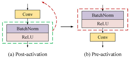
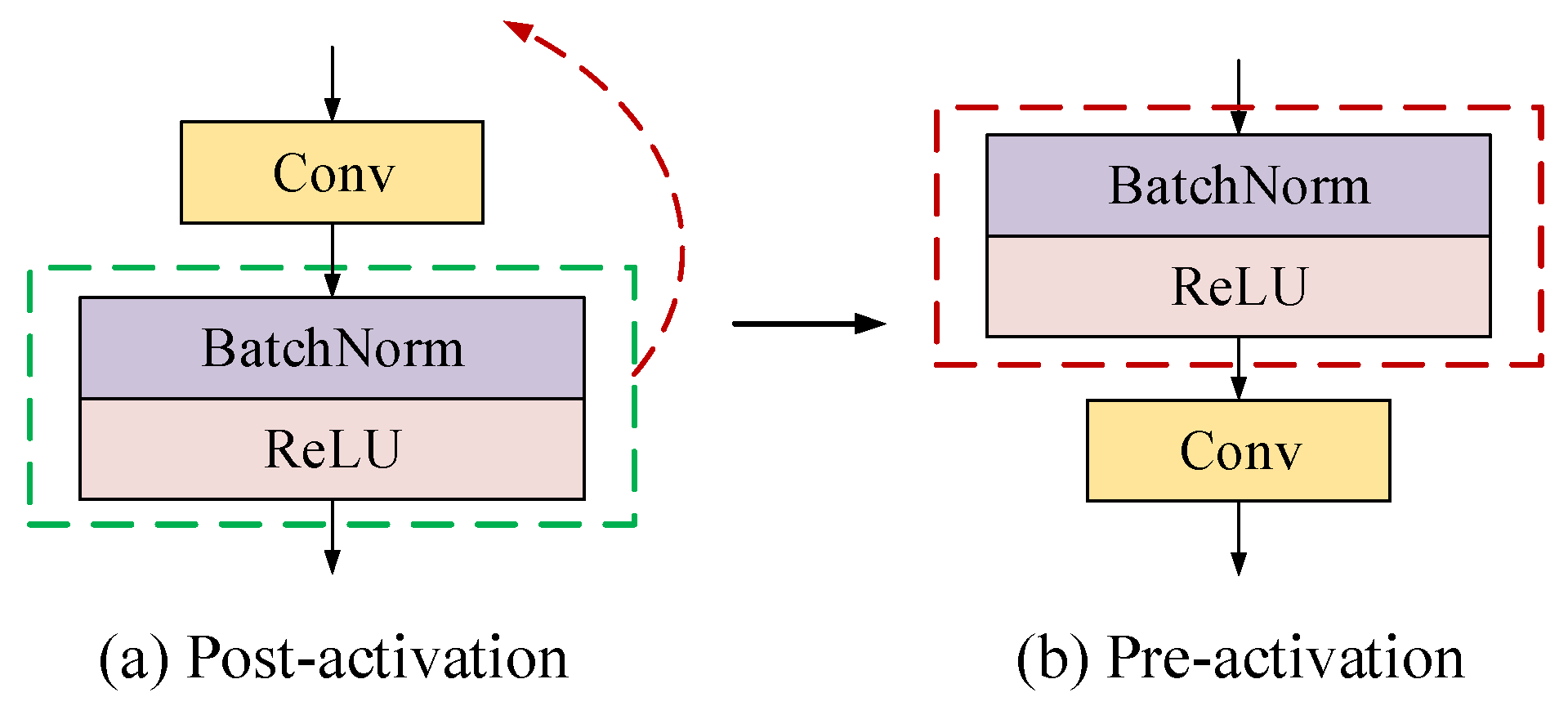
Typically, neural networks adopt a post-activation architecture, where nonlinear activation functions and normalization operations are applied subsequent to the linear transformation of neural network layers. Its core characteristic lies in the sequential implementation of three steps: first conducting feature transformation, then introducing expressive capacity via nonlinear activation, and finally performing normalization to stabilize training. However, in post-activation, gradients in deep networks are prone to sharp attenuation in magnitude due to the combined effects of activation functions and repeated linear transformations. Furthermore, in the post-activation paradigm, the input to the linear transformation consists of raw features, which often leads to training divergence or slow convergence due to excessive differences in feature magnitudes [22].

As shown in Figure 1, pre-activation places normalization operations and nonlinear activation functions prior to linear transformation, overcoming the inherent limitations of post-activation in terms of gradient propagation and training stability [23]. On one hand, normalization standardizes input features in advance, preventing gradients from being amplified or compressed by outliers during backpropagation. On the other hand, the pre-activation’s preprocessing sequence (normalization followed by activation) ensures that the input to the linear transformation maintains a standardized distribution, reducing sensitivity to weight initialization and learning rate selection, thereby enhancing training stability [24].

Figure 1. Post-activation and Pre-activation.

2.2. BiGRU

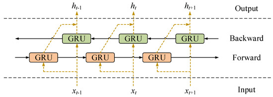
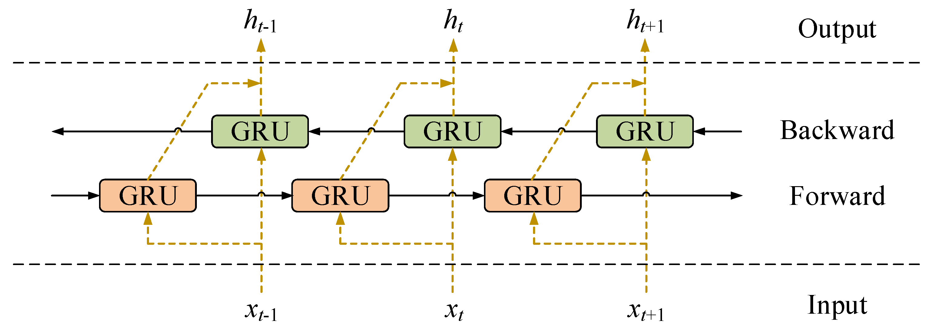
Bidirectional Gated Recurrent Unit (BiGRU) is an extended variant of the Gated Recurrent Unit (GRU) that integrates forward and backward sequential information modeling. By constructing forward GRU and backward GRU, it captures the dependencies between historical and future contextual information of sequence data, which overcomes the limitation of traditional RNNs and single-directional GRUs that only process sequences in one direction [25]. This characteristic makes BiGRU particularly suitable for time-series analysis tasks, where the current state of the system is often jointly determined by past operating conditions and subsequent response signals.

The core mechanism of BiGRU inherits the gating structure of GRU, which includes two key gates: a reset gate and an update gate. These gates dynamically adjust the flow of information in the network, effectively alleviating the gradient vanishing and exploding problem in long-sequence training. Figure 2 illustrates the structure of BiGRU.

Figure 2. The structure of BiGRU.

3. Proposed Method

3.1. Residual Parallel Convolutional Block

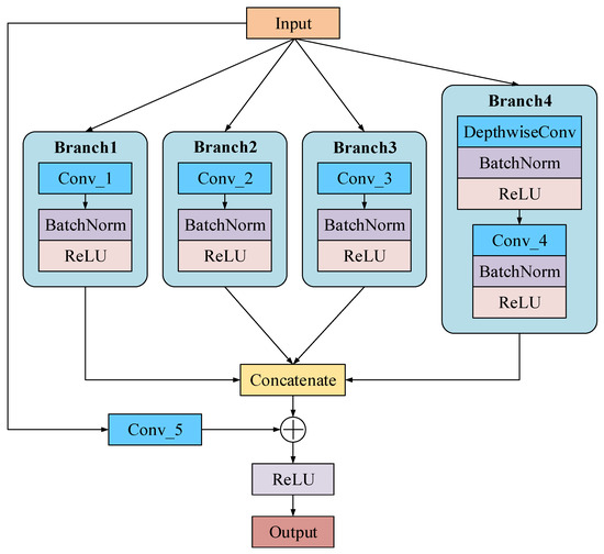
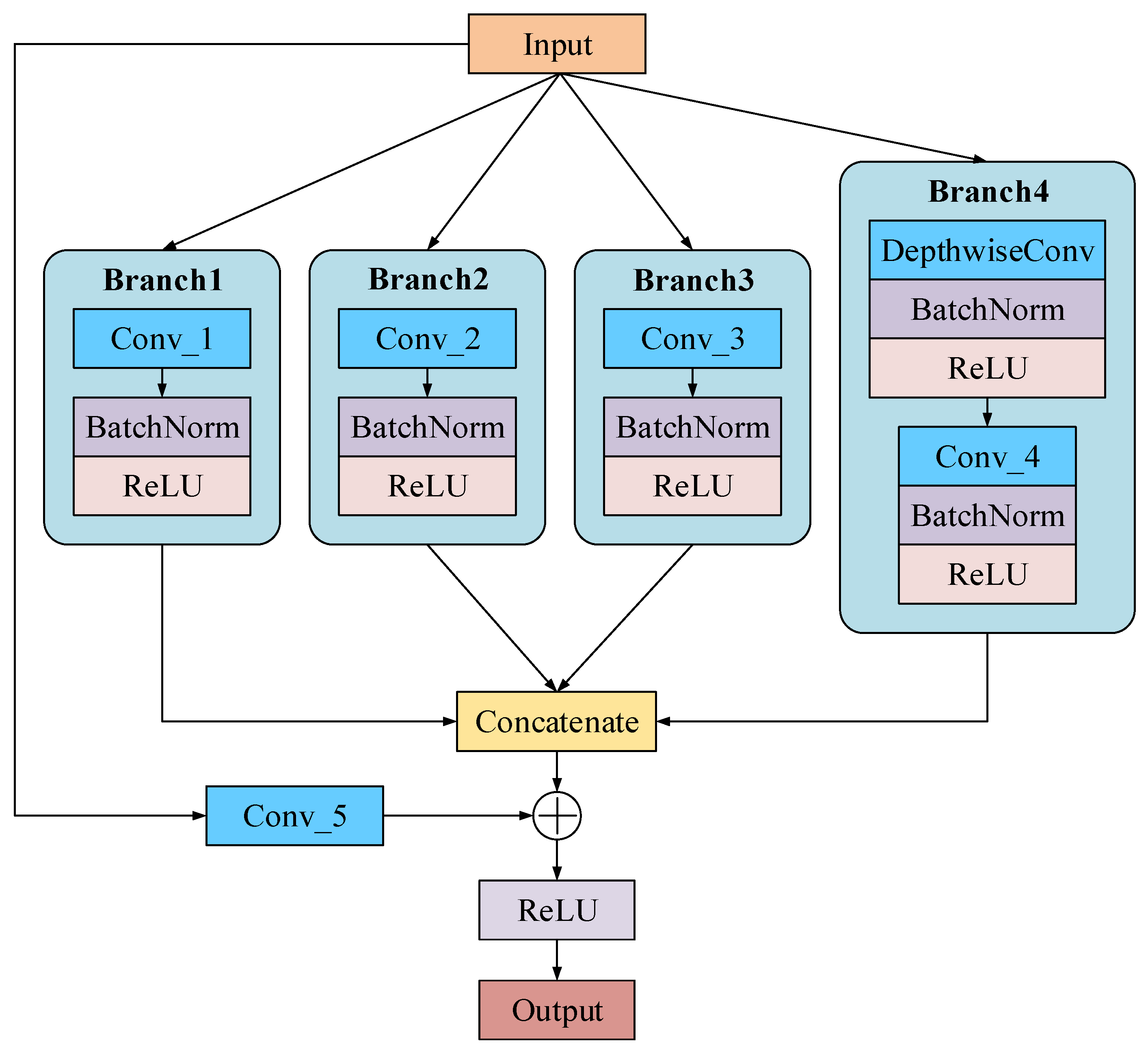
To enhance the model’s performance for capturing multi-scale degradation features and mitigate gradient degradation in deep architectures, we propose a residual parallel convolutional block (RPCB). Inspired by the Inception architecture, this module employs four parallel branches to simultaneously extract features at different scales. This structure is shown in Figure 3 and the parameter settings are listed in Table 1.

Figure 3. The structure of the residual parallel convolutional block.

Table 1. The parameter settings of the RPCB.

Layer	In_Channel	Out_Channel	Other Parameters
Conv_1	64	32	Kernel size: 1 Padding: 0
Conv_2	64	32	Kernel size: 3 Padding: 1
Conv_3	64	32	Kernel size: 5 Padding: 2
DepthwiseConv	64	64	Kernel size: 3 Padding: 1
Conv_4	64	32	Kernel size: 1 Padding: 0

Given the input data $X\in {ℝ}^{C_{in}\times T}$, where $C_{in}$ denotes the number of input channels and T represents the sequence length, the module first uniformly distributes the number of output channels $C_{out}$ to each branch. Branch 1 utilizes a 1 × 1 convolution for channel-wise linear transformation:

$$Y_1=ReLU\left(BN\left(W_1^{\left(1\right)}\ast X+b_1\right)\right)$$

(1)

To capture local and broader contextual information, respectively, branches 2 and 3 apply standard 3 × 3 and 5 × 5 convolutions with appropriate padding to preserve sequence length:

$$Y_2=ReLU\left(BN\left(W_2^{\left(3\right)}\ast X+b_2\right)\right)$$

(2)

$$Y_3=ReLU\left(BN\left(W_3^{\left(5\right)}\ast X+b_3\right)\right)$$

(3)

Branch 4 adopts a depth-wise separable convolution: a depth-wise 3 × 3 convolution models intra-channel temporal dependencies, followed by a point-wise 1 × 1 convolution to fuse cross-channel information, achieving high representational efficiency with reduced computational cost:

$$Z=ReLU\left(BN\left(W_d^{\left(3\right)}\ast X+b_d\right)\right)$$

(4)

$$Y_4=ReLU\left(BN\left(W_4^{\left(1\right)}\ast X+b_4\right)\right)$$

(5)

The four output branches are concatenated along the channel dimension to form a multi-scale feature representation:

$$F\left(X\right)=Y_1\oplus Y_2\oplus Y_3\oplus Y_4$$

(6)

To further improve gradient flow and training stability, a residual connection is added between the input and output of the block. When the input and output channel dimensions differ, a 1 × 1 convolutional projection is applied to align the dimensions:

$$P\left(X\right)=\left\{\begin{array}{c}X,C_{in}=C_{out}\\ BN\left(W_s^{\left(1\right)}\ast X+b_s\right),otherwise\end{array}\right.$$

(7)

Formally, the output is given by:

$$Y=ReLU\left(F\left(X\right)+P\left(X\right)\right)$$

(8)

where X is the input, ∗ represents the convolutional operation, $W^{\left(k\right)}$ denotes a convolutional kernel with a kernel size of k, and $\oplus$ is the channel concatenation along the channel dimension.

This design synergistically combines multi-scale feature extraction with residual learning, enhancing both representational power and convergence behavior.

3.2. Pre-Activated Convolutional Structure

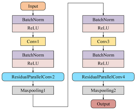
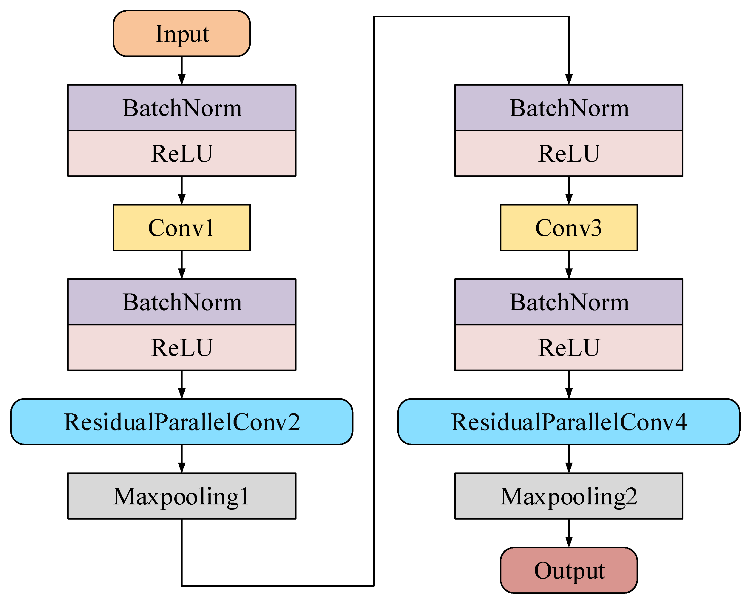
The backbone of the proposed model in this study adopts a pre-activated hierarchical convolutional network, which is designed to hierarchically extract high-dimensional temporal feature representations from raw time series. This network adheres to the pre-activation design paradigm, where Batch Normalization and ReLU activation function are sequentially applied prior to each convolution operation to enhance gradient propagation and improve training stability [26]. The structure is shown in Figure 4 and the parameter settings are listed in Table 2.

Figure 4. Pre-activated convolutional structure.

Table 2. The parameter settings of the pre-activated convolutional structure.

Layer	In_Channels	Out_Channels	Other Parameters
Conv1	14	64	Kernel size: 3 Padding: 1
ResidualParallelConv2	64	128	/
Maxpooling1	128	128	Kernel size: 2 Stride: 2
Conv3	128	256	Kernel size: 3 Padding: 2
ResidualParallelConv4	256	512	/
Maxpooling2	512	512	Kernel size: 2 Stride: 2

The input data is first transposed and adapted to the input format of convolution. Subsequently, the data is processed through two cascaded feature extraction stages:

Stage1: The input is processed by a standard 3 × 1 convolutional layer that maps it to a 64-dimensional feature space. This is followed by a residual parallel convolutional block, which enriches local temporal representations while preserving gradient integrity through skip connections. The output channel count is expanded to 128. A subsequent max-pooling layer with kernel size of 2 reduces the temporal resolution by half, thereby enlarging the effective receptive field.

Stage2: The downsampled features are further processed by a 3 × 1 convolution kernel and then fed into the second residual parallel convolutional block. This module further expands the number of channels to 512, followed by max-pooling to achieve temporal compression.

This architecture effectively captures multi-level temporal dependencies from local to global scales by integrating pre-activated convolution and residual parallel convolutional blocks, providing robust and information-rich feature representations for subsequent sequence modeling.

3.3. The Framework of the Proposed PRPC-BiGRU

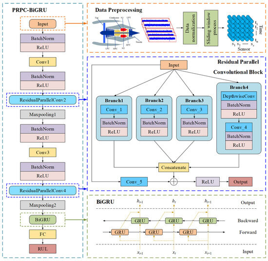
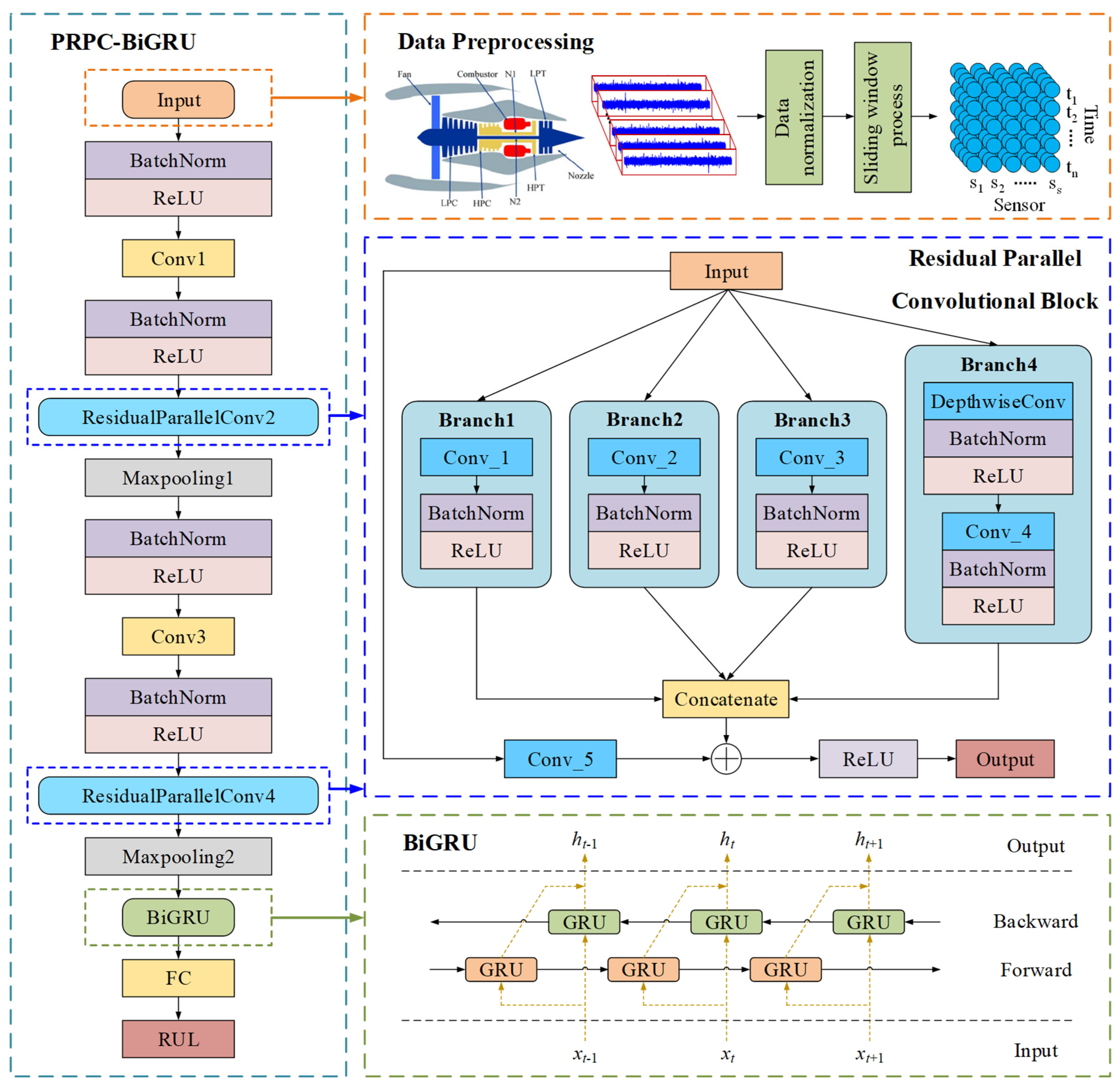
Based on the above descriptions of the model structure and key components, the RUL prediction framework of the proposed PRPC-BiGRU is systematically shown in Figure 5. It primarily comprises three steps:

Figure 5. The framework of PRPC-BiGRU.

Step1 is data processing. First, sensor signals with significant variations are selected from the sensor data based on their variation trends, and the filtered sensor signals are subjected to normalization processing. Then, the sliding window technique is utilized to split the processed data into equal-length sequences, where a sliding window of length 30 is adopted in this study.

Step2 is model construction. The RUL labels on the partitioned training dataset are served as inputs to the prediction model for training. We constructed a pre-activated convolutional structure to hierarchically extract high-dimensional temporal feature representations from raw time series, and the residual parallel convolutional block is introduced into it to enhance the model’s capacity for extracting multi-scale degradation features. The output of the pre-activated convolutional structure is then input into BiGRU and the fully connected layers ultimately produce the RUL prediction results as the output.

Step3 is RUL prediction and visualization. To evaluate the model’s performance, the trained model is tasked with predicting on the test dataset. The prediction results are first visualized for intuitive observation and then systematically compared with the true values.

4. Experiment and Model Analysis

4.1. Case Ⅰ: RUL Prediction of Aero-Engines

4.1.1. Data Description and Preprocessing

The Commercial Modular Aero Propulsion System Simulation (CMAPSS) dataset was used to validate the effectiveness of the proposed model, which was a simulated degradation dataset for commercial aero-turbine engines released by NASA [27]. To monitor engine conditions, 21 physical sensors were deployed at different locations, measuring parameters such as temperature, pressure, and rotational speed.

The CMAPSS dataset consisted of four subsets, designated as FD001, FD002, FD003, and FD004. With 26 data columns in each subset, the included variables covered the engine unit number, degradation cycle count, three operational setting parameters, and 21 real sensor signals. Table 3 shows the information of the four subsets. Each subset is further divided into a training set and a test set: the training set included actual sensor signals throughout the entire lifecycle of the turbofan engines, while the test set only contained actual sensor signals from a period prior to engine degradation. Overall, 7 out of the 21 sensor signals remained almost constant throughout the engine lifecycle [28], and these signals were discarded to eliminate irrelevant information. According to the literature [29], the 14 sensor signals that exhibited increasing and decreasing trends were retained as raw data. This retention was based on the premise that these signals were likely to contain more valuable degradation-related information.

Table 3. Basic information of the CMAPSS dataset.

Dataset	FD001	FD002	FD003	FD004
Training engines	100	260	100	249
Testing engines	100	259	100	248
Operation conditions	1	6	1	6
Fault modes	1	1	2	2

Significant magnitude differences existed among the raw sensor signals in the CMAPSS dataset. To unify data dimensions and accelerate model convergence, the Z-SCORE normalization strategy was employed to normalize the raw sensor signals [30]. In addition, the sliding window method was adopted to construct segmented samples, aiming to enhance the degradation information contained in the samples and facilitate the model in capturing temporal dependencies within the degradation data. This method involved sliding a fixed-size time window over the data sequence to extract local data segments. To capture temporal dependencies in degradation data, we used an overlapping sliding window to segment the normalized time-series data into fixed-length sequences. Using a step size of one maximized the retention of temporal continuity between adjacent sequences and enabled the acquisition of sufficient data samples.

4.1.2. Experimental Settings

We conducted all experiments on an NVIDIA GeForce RTX 3090 GPU, where the implementation was built on Python 3.9 with the PyTorch 1.9.0 framework.

We have presented all hyperparameters of the model training process in the following Table 4. In the training process, a learning rate decay strategy was employed during training: the initial learning rate was set to 0.2, and it decayed to 10% of its original value every ten epochs in the training phase. To mitigate overfitting, a dropout layer was incorporated with a dropout rate of 0.5. We selected the Root Mean Square Error (RMSE) as the loss function to calculate the training loss, while utilizing the RMSprop optimizer to optimize the network parameters. In addition, the piece-wise linear degradation principle was employed to construct the RUL labels, with the maximum RUL of the aircraft engines fixed at 125 flight cycles.

Table 4. The experimental settings for the model training process.

Hyperparameter	Value
Initial learning rate	0.2
Batch size	128
Training epoch	30
Dropout rate	0.5
Optimizer	RMSprop

To evaluate the prediction performance of PRPC-BiGRU, two metrics were adopted:

(1)

The RMSE served to quantify the average discrepancy between the predicted and actual RUL, with its definition formulated below:

$$RMSE=\sqrt{{\displaystyle \frac{1}{n}}{\displaystyle \sum _{i=1}^n{({\widehat{Y}}_i-Y_i)}^2}}$$

(9)

(2)

The Score assigns a higher penalty to delayed estimations compared to earlier estimations, and it can be computed in the following way:

$$Score=\left\{\begin{array}{c}{\displaystyle \sum _{i=1}^n(e^{-\frac{{\widehat{Y}}_i-Y_i}{13}}-1)},{\widehat{Y}}_i<Y_i\\ {\displaystyle \sum _{i=1}^n(e^{\frac{{\widehat{Y}}_i-Y_i}{10}}-1)},{\widehat{Y}}_i\ge Y_i\end{array}\right.$$

(10)

where n is the number of samples, while ${\widehat{Y}}_i$ and $Y_i$ denote the predicted and actual RUL for the ith sample, respectively.

4.1.3. Experimental Results and Comparisons

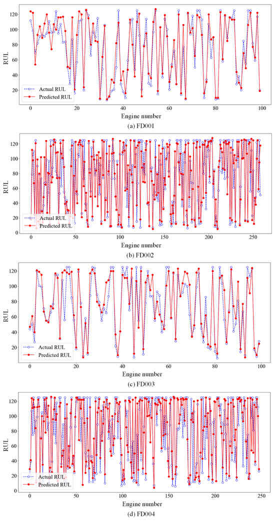
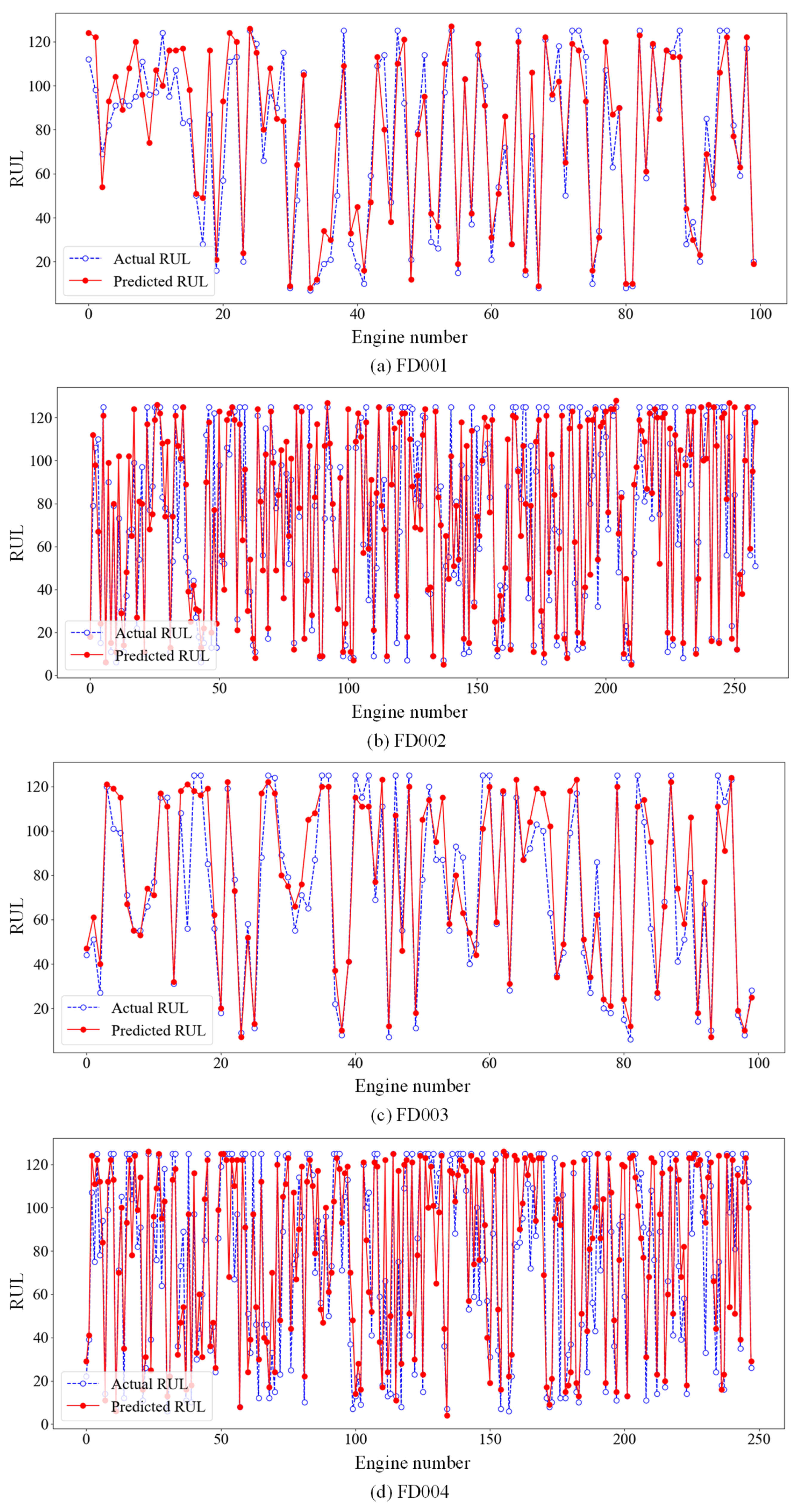
The RUL values and their corresponding actual RUL results for all test aero-engines across the four designated subsets were visually presented in Figure 6. As shown in Figure 6, it can be clearly observed that the predicted RUL curves exhibited a high degree of consistency with the actual RUL trajectories; most predicted values were tightly clustered around the actual values, and the deviations between them were confined within a reasonable range. This favorable matching performance fully demonstrated that the proposed model was capable of accurately capturing the inherent degradation trends of aero-engines, even when faced with variations across different subsets. Consequently, it validated the effectiveness of PRPC-BiGRU in RUL prediction.

Figure 6. The RUL prediction results of the proposed model.

To further verify the superiority and performance advantages of our proposed method, we compared our proposed method with additional state-of-the-art methods. The results of RMSE and Score are shown in Table 5 and Table 6. The advanced methods published in the past three years were selected for comparison to verify the advancement of the proposed method. The comparison results demonstrated that the proposed method achieved high prediction accuracy in each sub-dataset, and its overall prediction accuracy across the four sub-datasets was the highest. Relative to the optimal approach, the RMSE and Score for FD002 dropped by 13.50% and 6.52%, with the corresponding metrics for FD004 declining by 2.20% and 12.03%. Given that FD002 and FD004 had the most complex operating conditions and posed the greatest prediction challenges, the proposed method’s highest prediction accuracy in these two datasets further validated its superior prediction performance.

Table 5. The RMSE of the proposed PRPC-BiGRU and the contrast methods. Numbers with the bold are the minimums.

Methods	FD001	FD002	FD003	FD004	Average
EAGDE [31], 2022	14.10	20.60	18.86	26.40	19.99
ABGRU [28], 2023	12.83	17.97	13.23	21.55	16.40
CapsNet [32], 2024	12.80	19.87	13.62	23.90	17.55
RCNN-BLSTM [33], 2024	12.54	17.63	13.36	20.54	16.02
GWO-1DCNN [34], 2025	13.76	23.08	15.51	N/A	17.45
PRPC-BiGRU	14.11	15.25	14.45	20.09	15.97

Table 6. The Score of the proposed PRPC-BiGRU and the contrast methods. Numbers with the bold are the minimums.

Methods	FD001	FD002	FD003	FD004	Average
EAGDE [31], 2022	253	3122	514	4795	2171
ABGRU [28], 2023	221	2072	279	3625	1549
CapsNet [32], 2024	292	3185	338	7404	2804
RCNN-BLSTM [33], 2024	239	2345	245	3326	1541
GWO-1DCNN [34], 2025	462	8147	608	N/A	3072
PRPC-BiGRU	334	1937	423	2926	1405

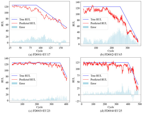
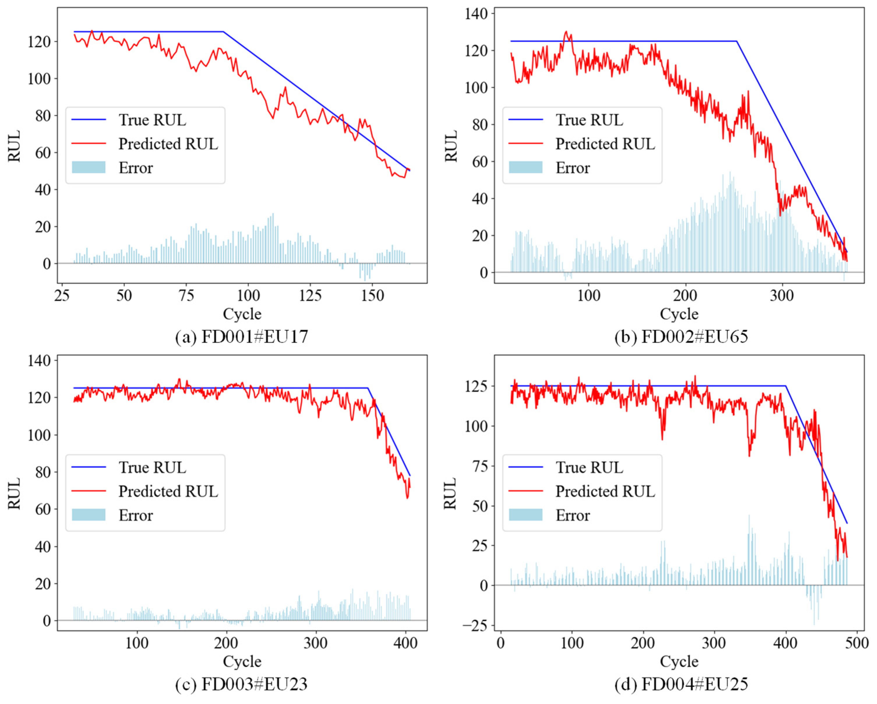
Four engine units were selected from the FD001–FD004 subsets of the CMAPSS dataset to visualize the continuous RUL prediction results, as presented in Figure 7. From these results, it can be observed that the proposed PRPC-BiGRU architecture can effectively capture the degradation features of engines. Shortly before the engine reached an end-of-life state, the predicted results were slightly lower than the actual values, thereby enabling the early detection of impending failures and facilitating proactive implementation of predictive maintenance. This can be crucial for ensuring the stable operation of aero-engines and reducing the occurrence of unexpected accidents.

Figure 7. The RUL prediction results of four engine units.

As can be seen from Figure 7, a certain degree of underestimation existed in the early stage. Since the degradation features were not obvious in this stage, the prediction deviation was relatively small. In the middle stage, degradation features became prominent and multiple degradation modes may exist, which increased the difficulty of prediction and led to larger prediction deviation, with underestimation still appearing as an overall trend. In the late stage, degradation accelerated and degradation features became more distinct, where prediction deviation gradually decreased and small fluctuations between underestimation and overestimation were observed.

4.1.4. Ablation Study

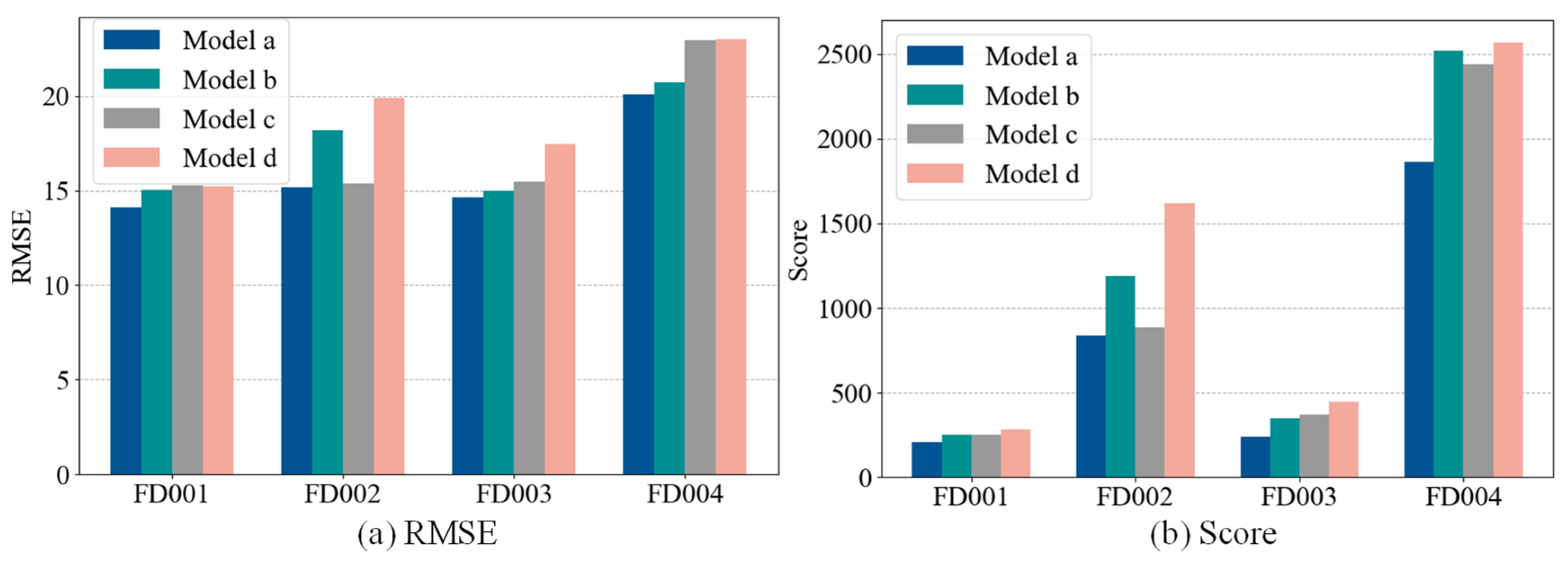
To effectively find out which part of the proposed PRPC-BiGRU contributed the most to model predictive performance and verify the importance of RPCB, an ablation study was performed across the four subsets of the CMAPSS dataset to assess the model’s predictive performance. Four models were conducted, namely, (1) Model a: pre-activated residual parallel convolutional block-based BiGRU; (2) Model b: residual parallel convolutional block-based BiGRU; (3) Model c: pre-activated BiGRU; and (4) Model d: BiGRU. The descriptions of models in the ablation study are listed in Table 7. The experimental settings were the same as the above experiments. Similarly, with RMSE and Score serving as the evaluation metrics, the prediction results are depicted in Figure 8.

Table 7. The description of the models in the ablation study.

Model	Description
Model a	Pre-activation + RPCB + BiGRU
Model b	RPCB + BiGRU
Model c	Pre-activation + BiGRU
Model d	BiGRU

Figure 8. The RUL prediction results of the ablation study.

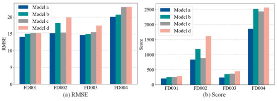
It can be observed from the prediction results that Model b, Model c, and Model d exhibited inferior prediction performance compared to Model a across all four datasets. It was noteworthy that the proposed PRPC-BiGRU model, which incorporated pre-activation and extracted multi-scale features, achieved the optimal prediction results across all four datasets; this highlights the superior prediction performance of the proposed method. Furthermore, both Model b (integrating RPCB) and Model c (incorporating pre-activation) outperformed Model d, which also validated the effectiveness of the RPCB module and pre-activation structure in enhancing the model’s prediction accuracy.

4.1.5. Analysis of Model Training Stability

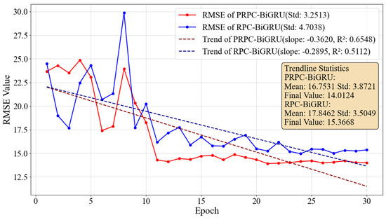
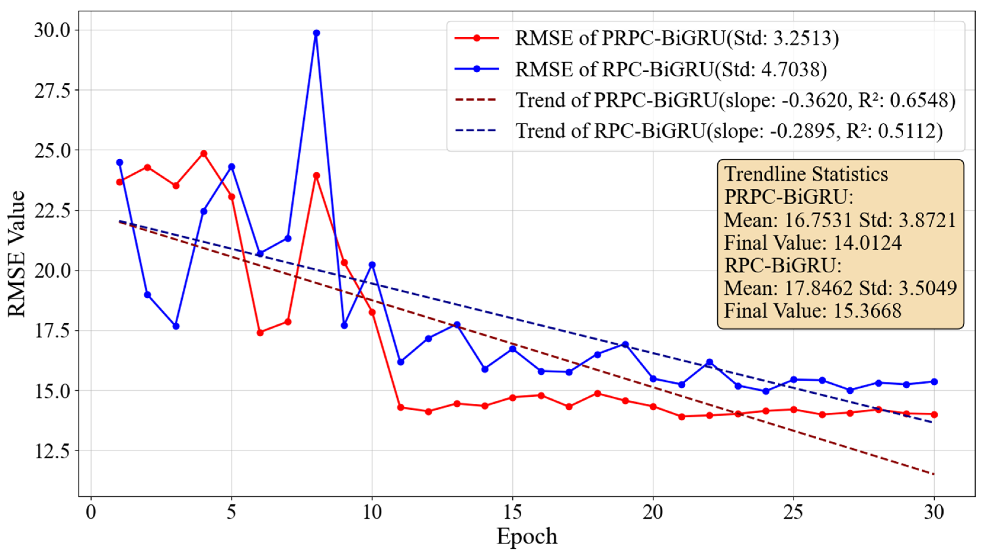
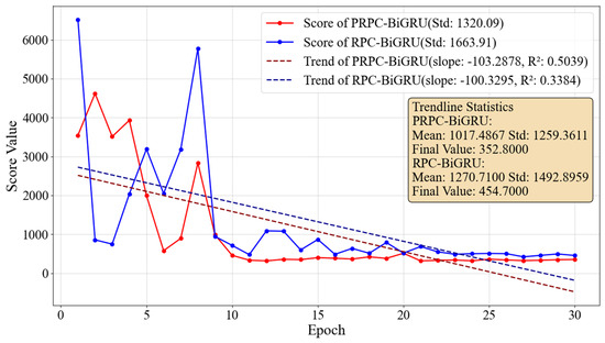
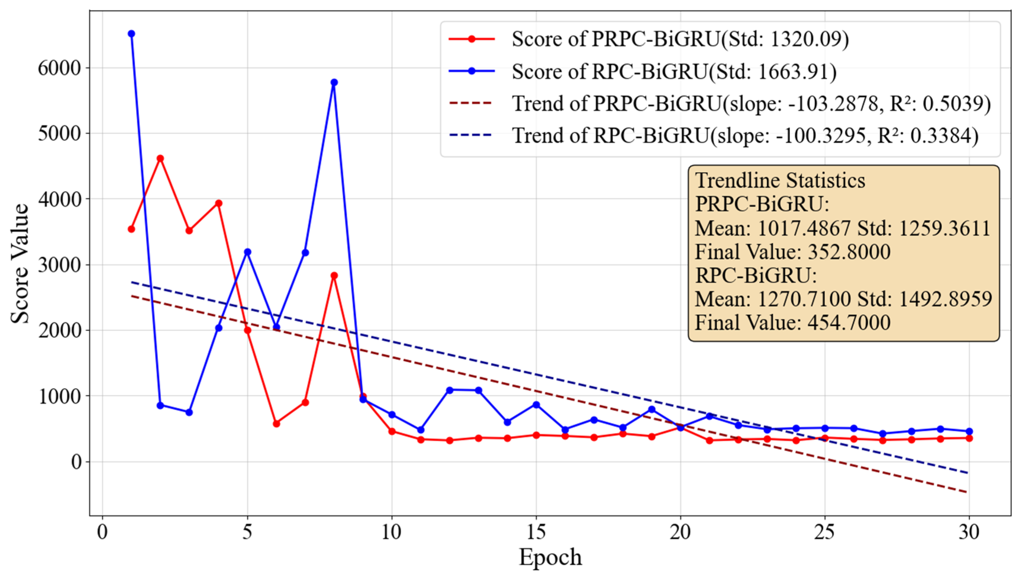
To verify the effectiveness of the pre-activation structure in improving model training stability, a training stability analysis was conducted on the FD001 dataset. The RMSE and Score values for each epoch during the training of PRPC-BiGRU and RPC-BiGRU (without pre-activation) were recorded, and their variation trends were visualized as shown in Figure 9 and Figure 10. It can be observed from these visualizations that both PRPC-BiGRU and RPC-BiGRU exhibited significant fluctuations in the first 10 epochs. After 10 epochs, the RMSE and Score of PRPC-BiGRU gradually stabilized with significantly reduced volatility, while RPC-BiGRU still showed certain fluctuations. To quantify the volatility, the standard deviations (Std) of their RMSE and Score were calculated, respectively, to measure the degree of dispersion between data points and their mean values. The results indicated that PRPC-BiGRU had a smaller standard deviation, demonstrating more stable prediction errors during training. Furthermore, PRPC-BiGRU’s RMSE and Score ultimately converged to lower values, reaffirming its superior prediction performance.

Figure 9. The changing trend of RMSE during the training process.

Figure 10. The changing trend of Score during the training process.

In addition, the trend lines of their RMSE and Score were plotted to represent the overall variation trends in the data. As shown in Figure 9 and Figure 10, both models’ RMSE and Score exhibited a clear downward trend. Meanwhile, the coefficients of determination (R²) of the trend lines were calculated to measure the proportion of sequence variation explained by the trend lines. Specifically, the closer R² is to 1, the more the data variation aligns with a linear trend; the closer R² is to 0, the more irregular the data variation [35]. The R² values of PRPC-BiGRU’s RMSE and Score were both higher than those of RPC-BiGRU, indicating that PRPC-BiGRU’s RMSE and Score decreased more steadily during training and had superior training stability. This was consistent with the inherent characteristics of the pre-activation structure, which optimized gradient flow and reduced training volatility.

4.2. Case Ⅱ: RUL Prediction of Milling Cutters

4.2.1. Data Description and Preprocessing

The run-to-failure datasets of cutting tools released by the PHM 2010 data challenge were used in this section to validate the effectiveness of the proposed method in real industrial equipment [36]. In each experiment, the cutter was used when machining the entire slope of the workpiece surface. The complete cycle of machining one surface and carrying out one measurement was defined as a time unit. Six cutting tools (C1 to C6) were used to collect six run-to-failure sub-datasets each containing data from seven sensors. Three experiments (C1, C4, and C6) were used in this article to demonstrate the proposed method. The Root Mean Square (RMS) values of the measurements were calculated as raw features. The Z-SCORE normalization was performed on the RMS sequences. The RMS sequences were segmented by a sliding time window with length of 30, and the obtained data was used as the input of the network. The time interval between the current moment of a sample and the failure moment was used as the RUL label of the sample. The failure moment was the time when the mean tool wear reached the failure threshold.

To make full use of the dataset, as shown in Table 8, any two of the three subsets were used as the training set to train the proposed model, and the remaining one was used as the test set to test the model’s performance.

Table 8. The information of tool wear monitoring dataset.

Training Set	Testing Set	Training Samples	Testing Samples
C1 + C4	C6	306 + 278 = 584	238
C1 + C6	C4	306 + 238 = 544	278
C4 + C6	C1	278 + 238 = 516	306

4.2.2. Performance Evaluation and Comparison

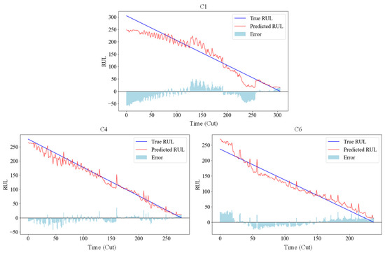
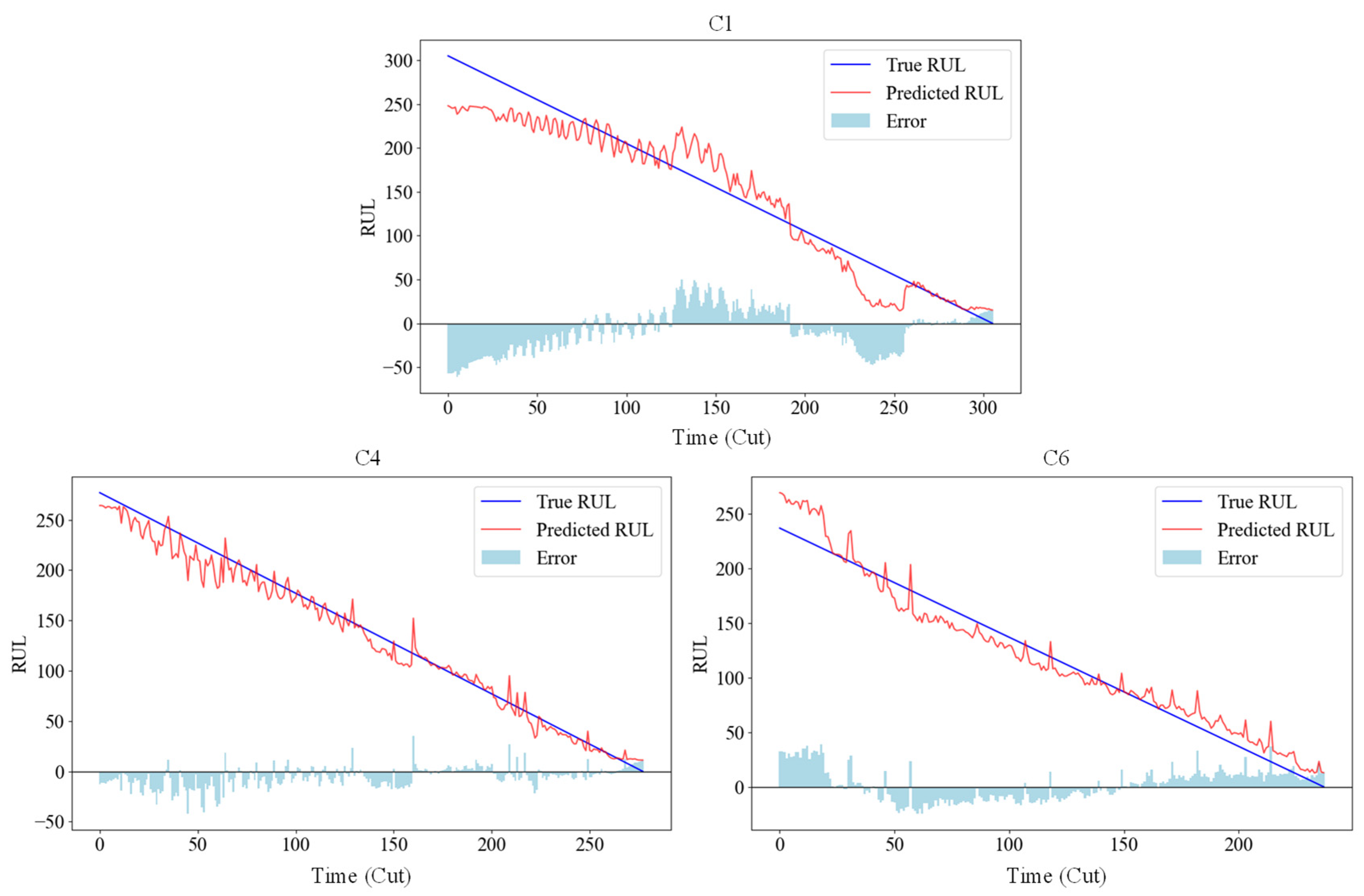
The predicted and actual RUL results of each cutter are shown in Figure 11. It can be found that the predicted RUL and the actual RUL had a good fitting effect.

Figure 11. The RUL prediction results of each dataset.

Table 9 lists the RUL prediction results of different comparison methods on the tool wear monitoring dataset. It can be seen from the results that the proposed method achieved better performance compared to other models in the C4 and C6 subsets in terms of RMSE and Score metrics. Additionally, our method also achieved the lowest average of RMSE and Score across the three subsets. This means that the proposed method has the best comprehensive performance compared with different comparison methods. It is worth noting that the PRPC-BiGRU still achieved satisfactory results in real industrial datasets.

Table 9. The RMSE and Score of the proposed PRPC-BiGRU. Numbers with the bold are the minimums.

Methods	C1		C4		C6		Average
	RMSE	Score	RMSE	Score	RMSE	Score	RMSE	Score
SSAE-BDT [37]	14.84	N/A	17.08	N/A	17.58	N/A	16.50	N/A
ATCN [38]	18.54	1759	13.96	900	16.04	1171	16.18	1277
DA-LSTM [39]	16.79	1412	14.07	945	17.93	1413	16.26	1257
PRPC-BiGRU	16.36	1402	13.71	761	15.38	567	15.15	910

5. Conclusions

In this study, a pre-activated residual parallel convolutional block-based BiGRU model was proposed for RUL prediction. To address the limitations of existing RUL prediction methods in multi-scale feature extraction and training stability, this study proposed the following innovations: First, a residual parallel convolutional block was developed, which employed four parallel branches to simultaneously extract features of different scales, effectively enhancing the model’s performance to capture multi-scale degradation features. Second, a pre-activation convolutional structure, which placed normalization and activation functions prior to convolution operations, was designed to significantly improve gradient propagation and enhanced training stability. Finally, the PRPC-BiGRU model was constructed by integrating the above innovative components, enabling high-precision RUL prediction.

Experimental results on aero-engine benchmark datasets demonstrated that the proposed method achieved excellent prediction performance across all four sub-datasets. Ablation experiments validated the significant contributions of the RPCB module and pre-activation structure to model performance, while training stability analysis further confirmed that the pre-activation structure could effectively reduce training volatility and accelerate convergence speed. Future work will explore the application of this model in RUL prediction tasks for other industrial equipment and further optimize the model structure to improve prediction accuracy.

References

- Miao, Y.; Li, C.; Zhang, B.; Lin, J. Application of a coarse-to-fine minimum entropy deconvolution method for rotating machines fault detection. Mech. Syst. Signal Process. 2023, 198, 110431. [Google Scholar]
- Shi, H.; Miao, Y.; Wang, X.; Xie, J. Application of a multi-dimensional synchronous feature mode decomposition for machinery fault diagnosis. ISA Trans. 2025, 160, 218–236. [Google Scholar] [CrossRef] [Scilit] [PubMed]
- Tang, J.; Miao, Y.; Xia, Y.; Zhou, Q.; Yi, C. A multi-scale pooling attention-based graph attention network for remaining useful life prediction. IEEE Trans. Instrum. Meas. 2025, 74, 3528914. [Google Scholar]
- Miao, Y.; Hu, S.; Liu, Y.; Hua, J. Angle-domain feature mode decomposition for fault diagnosis under speed-varying condition. IEEE Trans. Instrum. Meas. 2025, 74, 3506909. [Google Scholar]
- Li, X.-Q.; Song, L.-K.; Bai, G.-C. Recent advances in reliability analysis of aeroengine rotor system: A review. Int. J. Struct. Integr. 2022, 13, 1–29. [Google Scholar]
- Paris, P.; Erdogan, F. A critical analysis of crack propagation laws. J. Basic Eng. 1963, 85, 528–533. [Google Scholar]
- Oppenheimer, C.H.; Loparo, K.A. Physically based diagnosis and prognosis of cracked rotor shafts. In Component and Systems Diagnostics, Prognostics, and Health Management II; SPIE: Orlando, FL, USA, 2002; pp. 122–132. [Google Scholar]
- Rivas, A.; Delipei, G.K.; Hou, J. Predictions of component remaining useful lifetime using Bayesian neural network. Prog. Nucl. Energy 2022, 146, 104143. [Google Scholar] [CrossRef] [Scilit]
- Tang, J.; Zheng, G.; He, D.; Ding, X.; Huang, W.; Shao, Y.; Wang, L. Rolling bearing remaining useful life prediction via weight tracking relevance vector machine. Meas. Sci. Technol. 2020, 32, 024006. [Google Scholar] [CrossRef] [Scilit]
- Alfarizi, M.G.; Tajiani, B.; Vatn, J.; Yin, S. Optimized random forest model for remaining useful life prediction of experimental bearings. IEEE Trans. Ind. Inform. 2022, 19, 7771–7779. [Google Scholar] [CrossRef] [Scilit]
- Fan, L.; Chai, Y.; Chen, X. Trend attention fully convolutional network for remaining useful life estimation. Reliab. Eng. Syst. Saf. 2022, 225, 108590. [Google Scholar] [CrossRef] [Scilit]
- Ren, L.; Sun, Y.; Wang, H.; Zhang, L. Prediction of bearing remaining useful life with deep convolution neural network. IEEE Access 2018, 6, 13041–13049. [Google Scholar] [CrossRef] [Scilit]
- Wen, L.; Su, S.; Li, X.; Ding, W.; Feng, K. GRU-AE-wiener: A generative adversarial network assisted hybrid gated recurrent unit with Wiener model for bearing remaining useful life estimation. Mech. Syst. Signal Process. 2024, 220, 111663. [Google Scholar] [CrossRef] [Scilit]
- Cheng, Y.; Qv, J.; Feng, K.; Han, T. A Bayesian adversarial probsparse Transformer model for long-term remaining useful life prediction. Reliab. Eng. Syst. Saf. 2024, 248, 110188. [Google Scholar] [CrossRef] [Scilit]
- Kim, S.; Seo, Y.-H.; Park, J. Transformer-based novel framework for remaining useful life prediction of lubricant in operational rolling bearings. Reliab. Eng. Syst. Saf. 2024, 251, 110377. [Google Scholar] [CrossRef] [Scilit]
- Huang, G.; Lei, W.; Dong, X.; Zou, D.; Chen, S.; Dong, X. Stage-based remaining useful life prediction for bearings using GNN and correlation-driven feature extraction. Machines 2025, 13, 43. [Google Scholar] [CrossRef] [Scilit]
- Miao, Y.; Xia, Y.; Chang, J. A variational autoencoder based lightweight physics-informed neural network for remaining useful life prediction. Meas. Sci. Technol. 2025, 36, 096125. [Google Scholar] [CrossRef] [Scilit]
- Yang, B.; Liu, R.; Zio, E. Remaining useful life prediction based on a double-convolutional neural network architecture. IEEE Trans. Ind. Electron. 2019, 66, 9521–9530. [Google Scholar] [CrossRef] [Scilit]
- Safavi, V.; Vaniar, A.M.; Bazmohammadi, N.; Vasquez, J.C.; Keysan, O.; Guerrero, J.M. Early prediction of battery remaining useful life using CNN-XGBoost model and Coati optimization algorithm. J. Energy Storage 2024, 98, 113176. [Google Scholar] [CrossRef] [Scilit]
- Yang, L.; Jiang, Y.; Zeng, K.; Peng, T. Rolling bearing remaining useful life prediction based on CNN-VAE-MBiLSTM. Sensors 2024, 24, 2992. [Google Scholar] [CrossRef] [Scilit]
- Yan, X.; Jin, X.; Jiang, D.; Xiang, L. Remaining useful life prediction of rolling bearings based on CNN-GRU-MSA with multi-channel feature fusion. Nondestruct. Test. Eval. 2024, 1–26. [Google Scholar] [CrossRef] [Scilit]
- Wang, H.; Yang, J.; Shi, L.; Wang, R. Remaining useful life prediction based on adaptive SHRINKAGE processing and temporal convolutional network. Sensors 2022, 22, 9088. [Google Scholar] [CrossRef] [Scilit]
- Akhlaghi, V.; Yazdanbakhsh, A.; Samadi, K.; Gupta, R.K.; Esmaeilzadeh, H. Snapea: Predictive early activation for reducing computation in deep convolutional neural networks. In 2018 ACM/IEEE 45th Annual International Symposium on Computer Architecture (ISCA); IEEE: Los Angeles, CA, USA, 2018; pp. 662–673. [Google Scholar]
- He, K.; Zhang, X.; Ren, S.; Sun, J. Deep residual learning for image recognition. In Proceedings of the IEEE Conference on Computer Vision and Pattern Recognition, Los Angeles, CA, USA, 27–30 June 2016; pp. 770–778. [Google Scholar]
- She, D.; Jia, M. A BiGRU method for remaining useful life prediction of machinery. Measurement 2021, 167, 108277. [Google Scholar] [CrossRef] [Scilit]
- Gao, H.; Yang, Y.; Yao, D.; Li, C. Hyperspectral image classification with pre-activation residual attention network. IEEE Access 2019, 7, 176587–176599. [Google Scholar] [CrossRef] [Scilit]
- Saxena, A.; Goebel, K.; Simon, D.; Eklund, N. Damage propagation modeling for aircraft engine run-to-failure simulation. In 2008 International Conference on Prognostics and Health Management; IEEE: Denver, CO, USA, 2008; pp. 1–9. [Google Scholar]
- Lin, R.; Wang, H.; Xiong, M.; Hou, Z.; Che, C. Attention-based gate recurrent unit for remaining useful life prediction in prognostics. Appl. Soft Comput. 2023, 143, 110419. [Google Scholar] [CrossRef] [Scilit]
- Lin, L.; Wu, J.; Fu, S.; Zhang, S.; Tong, C.; Zu, L. Channel attention & temporal attention based temporal convolutional network: A dual attention framework for remaining useful life prediction of the aircraft engines. Adv. Eng. Inform. 2024, 60, 102372. [Google Scholar]
- Miao, Y.; Xia, Y.; Liu, J. Remaining useful life prediction via a double convolutional attention-based CNN-GRU model. IEEE Trans. Instrum. Meas. 2025, 74, 3544313. [Google Scholar] [CrossRef] [Scilit]
- Abdelghafar, S.; Khater, A.; Wagdy, A.; Darwish, A.; Hassanien, A.E. Aero engines remaining useful life prediction based on enhanced adaptive guided differential evolution. Evol. Intell. 2024, 17, 1209–1220. [Google Scholar] [CrossRef] [Scilit]
- Li, D.; Chen, J.; Huang, R.; Chen, Z.; Li, W. Sensor-aware CapsNet: Towards trustworthy multisensory fusion for remaining useful life prediction. J. Manuf. Syst. 2024, 72, 26–37. [Google Scholar] [CrossRef] [Scilit]
- Yan, X.; Liang, W.; Sun, S. An improved method for predicting the remaining useful life using a spatial–temporal feature extraction network with attention mechanism. IEEE Access 2024, 12, 66587–66604. [Google Scholar] [CrossRef] [Scilit]
- Shen, L.; Wang, Y.; Du, B.; Yang, H.; Fan, H. Remaining Useful Life Prediction of Aero-Engine Based on Improved GWO and 1DCNN. Machines 2025, 13, 583. [Google Scholar] [CrossRef] [Scilit]
- Menard, S. Coefficients of determination for multiple logistic regression analysis. Am. Stat. 2000, 54, 17–24. [Google Scholar] [CrossRef] [Scilit]
- Li, X.; Lim, B.; Zhou, J.; Huang, S.; Phua, S.; Shaw, K.; Er, M.J. Fuzzy neural network modelling for tool wear estimation in dry milling operation. Annu. Conf. PHM Soc. 2009, 1, 1–11. [Google Scholar]
- Qin, Y.; Liu, X.; Yue, C.; Zhao, M.; Wei, X.; Wang, L. Tool wear identification and prediction method based on stack sparse self-coding network. J. Manuf. Syst. 2023, 68, 72–84. [Google Scholar] [CrossRef] [Scilit]
- Zhang, Q.; Liu, Q.; Ye, Q. An attention-based temporal convolutional network method for predicting remaining useful life of aero-engine. Eng. Appl. Artif. Intell. 2024, 127, 107241. [Google Scholar] [CrossRef] [Scilit]
- Shi, J.; Zhong, J.; Zhang, Y.; Xiao, B.; Xiao, L.; Zheng, Y. A dual attention LSTM lightweight model based on exponential smoothing for remaining useful life prediction. Reliab. Eng. Syst. Saf. 2024, 243, 109821. [Google Scholar] [CrossRef] [Scilit]
Disclaimer/Publisher’s Note: The statements, opinions and data contained in all publications are solely those of the individual author(s) and contributor(s) and not of MDPI and/or the editor(s). MDPI and/or the editor(s) disclaim responsibility for any injury to people or property resulting from any ideas, methods, instructions or products referred to in the content. |
© 2026 by the authors. Licensee MDPI, Basel, Switzerland. This article is an open access article distributed under the terms and conditions of the Creative Commons Attribution (CC BY) license.