A Data-Driven Approach for Energy Consumption Modeling and Optimization of Welding Robot Systems

Abstract

Welding robots play a crucial role in manufacturing industries, where minimizing energy consumption (EC) is increasingly important for enhancing efficiency and reducing operational costs. This study presents a data-driven approach to model and optimize EC in welding robot systems, utilizing a dataset generated from real-world measurements of robot EC during various motions and integrated with trajectory data. A predictive model was developed using an extreme gradient boosting (XGBoost) regression technique focused on joint torque data, which achieved a mean absolute percentage error (MAPE) of 1.86%. Furthermore, trajectory optimization was achieved by adjusting the spatial position of the workpiece, effectively reducing EC. To solve the optimization problem, an improved whale optimization algorithm (IWOA) was employed. Experimental validations with a welding robot demonstrate that the proposed method not only accurately predicted EC with a MAPE of 2.66% but also reduced the robot system’s EC by 6.72%, outperforming the traditional method focused solely on joint motor EC, which achieved a 4.08% reduction. These results confirm the efficacy of the proposed approach, underscoring its potential for broad application in robotic systems to achieve significant energy savings.

1. Introduction

Welding robots are extensively utilized in industries such as automotive manufacturing, shipbuilding, and bridge construction, owing to their high precision, repeatability, and stability [1,2]. Welding is a critical process in manufacturing, and the widespread adoption of welding robots has substantially increased EC [3]. In the context of rising global energy demand and costs, there is a pressing need for sustainable development and climate change mitigation; optimizing the EC of welding robots is essential to reduce manufacturing costs, mitigate carbon emissions, and enhance energy efficiency [4,5,6].

Two primary methods for establishing EC models for robotic systems are commonly used: the direct method and the indirect method [7]. The direct method calculates EC based on the dynamic characteristics of the robot [8,9]. Meike et al. [10] developed an EC model for the entire system by integrating the mechanical power of the drive motor and the power of the electric drive system, considering both robot motion and standstill conditions. Zhou et al. [11] proposed an EC model for industrial robots (IRs) by analyzing the dynamic characteristics of each joint, incorporating friction and motor losses, and combining joint velocity and acceleration trajectories. Li et al. [12] calculated joint torque using dynamic equations and considered mechanical power, electrical losses, and friction losses to compute the input power of permanent magnet synchronous motors (PMSMs), integrating this with the power consumption of other components via an energy integration model to calculate total robot EC. As IR systems become more complex, EC modeling methods based on kinematics and dynamics are often inadequate in accurately capturing certain energy components.

The indirect method combines robot motion parameters with machine learning models [13,14]. Zhang et al. [15] employed a back-propagation neural network (BPNN) to establish the quantitative relationship between operational parameters and EC. They later proposed a transfer learning-based approach to create EC models for IRs, improving modeling efficiency and accuracy in small sample size scenarios by adjusting multi-layer perceptron structure strategies [16]. A deep neural network based on long short-term memory (LSTM) was used to construct a nonlinear relationship between EC and joint motion variables, namely joint position, velocity, and acceleration, allowing EC to be predicted without the need for industrial robot parameters [17]. Lin et al. [18] utilized a data-driven method based on a batch normalization LSTM (BN-LSTM) network to develop an EC model for IR operations, demonstrating significant performance improvements over other machine learning and deep learning models. Data-driven methods for modeling EC bypass complex dynamics, offering a more reliable and accurate approach [19].

Accurate EC modeling provides a foundation for the energy-saving optimization of robot systems. Methods to reduce EC in IRs include developing energy-saving motion planning algorithms, optimizing operational parameters, and improving operational schedules [20]. Energy-saving motion planning algorithms generate robot motion trajectories with reduced EC. Luo et al. [21] proposed a trajectory planning method for optimizing the path tracking of IRs by combining interval analysis, segmented planning, and genetic algorithms to determine the optimal pose of the target path relative to the world coordinate system, thereby reducing EC. Optimizing operational parameters, such as joint velocity and acceleration, enables robots to minimize EC while fulfilling task requirements [9]. Li et al. [22] employed the sequential quadratic programming (SQP) method to address the nonlinear optimization problem of robot trajectory EC, achieving smooth motion and EC reduction by minimizing jerk values. Gadaleta et al. [23] optimized EC by adjusting joint velocities and accelerations, with the calculated parameters used to generate energy-optimal robot codes. Optimizing operational schedules involves efficiently arranging the working and idle times of robots to avoid unnecessary waiting and EC. Wang et al. [24] used a multi-objective particle swarm optimization algorithm (CG-MOPSO) combined with geometric obstacle avoidance strategies to optimize the path length of spot welding robots, enhancing welding efficiency and reducing EC. However, when the IR control system does not permit trajectory parameter adjustments and the path is predefined, traditional methods based on parameter optimization and schedule optimization have limited applicability.

Existing studies predominantly rely on traditional physics-based models for EC calculation, which fail to adequately capture the complex nonlinear dynamics and various energy loss components in robotic systems. Moreover, some optimization methods focus exclusively on reducing the mechanical output power of robot joints, overlooking internal losses within motors and transmission systems, resulting in suboptimal energy efficiency improvements. While data-driven approaches have been explored, such as BPNN [15], LSTM [17], and BN-LSTM [18], these methods often face several limitations in industrial applications. They typically require large, clean, and continuous datasets, which are difficult to obtain in dynamic and noisy industrial environments. Moreover, their computational complexity and black-box nature hinder real-time deployment and interpretability, which are critical factors in industrial robot systems [16,19]. As a result, their application in real-world industrial settings remains constrained by data acquisition challenges, model simplifications, and concerns regarding generalization to varying operational conditions.

To overcome these challenges, a novel data-driven approach for EC modeling and optimization in welding robot systems is proposed. An XGBoost regression model is developed for EC prediction, incorporating joint torques and other critical parameters, which offers a more accurate representation of system energy consumption compared to traditional physics-based methods. Furthermore, an IWOA is introduced to optimize both the workpiece position and robot motion planning, thus reducing overall energy consumption. This approach considers mechanical power and internal losses while optimizing the welding path layout, resulting in substantial energy savings. Experimental results demonstrate that the proposed method reduces total energy consumption by 6.72%, outperforming traditional methods focused solely on optimizing motor power consumption.

The remaining sections of this paper are organized as follows: Section 2 discusses the process of establishing the EC model for the welding robot system, Section 3 presents strategies and methods for reducing EC, and Section 4 provides experimental validation using specific workpieces.

2. Welding Robot EC Modeling

2.1. EC Analysis of Welding Robot System

Welding robots are primarily categorized into two types: laser welding and arc welding, both utilizing fundamentally similar IR carriers. This investigation focuses on arc welding robots. Figure 1 illustrates a typical arc-welding robot system consisting of an IR, welding machine, drive system, control system, and auxiliary components. The control system translates end-effector or joint motion commands into continuous joint motion signals, which are subsequently transmitted to the drive system. This transmission enables the control of joint motor movements, facilitating the attainment of instructed positions and the execution of intended actions. The IR predominantly consists of mechanical components, reduction gears, and PMSMs. Auxiliary components encompass a teach pendant, I/O board, switching power supply, cooling fans, and additional peripheral devices.

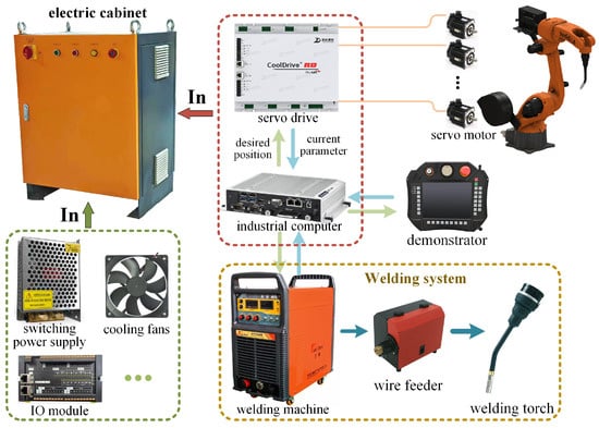
Figure 1. Detailed composition of the arc welding robot system.

Currently, IRs generally employ PMSMs as joint actuators, with an energy efficiency of around 90% [25]. The output shafts of the joint motors are connected to reducers (planetary gear reducers or harmonic drive reducers) to provide torque amplification and speed reduction. Equation (1) gives the mechanical output power of the joint motors.  

$$P_{m,m}={\tau }_i·{\dot{\theta }}_i$$

(1)

where $P_{m,m}$ represents the mechanical power output of the motor, which includes frictional losses caused by the reducer and the mechanical energy transmitted to the link end; ${\tau }_i$ denotes the torque of the i-th joint, and ${\dot{\theta }}_i$ represents the angular velocity of the i-th joint.

The general form of the robot dynamics model established using the Newton–Euler iterative method is as follows:

$$\mathit{\tau }=\mathit{M}\left(\theta \right)\ddot{\theta }+\mathit{C}(\theta ,\dot{\theta })\dot{\theta }+\mathit{G}\left(\theta \right)+{\mathit{\tau }}_f$$

(2)

where $\mathit{\tau }$ represents the generalized joint torques of the robot, n is the number of robot joints; $\theta ,\dot{\theta },\ddot{\theta }$ denote the joint angles, angular velocities, and angular accelerations, respectively; $\mathit{M}\left(\theta \right)\ddot{\theta }$ is the inertia torque; $\mathit{C}(\theta ,\dot{\theta })\dot{\theta }$ represents the Coriolis and centrifugal torques; $\mathit{G}\left(\theta \right)$ is the gravity torque, which depends solely on the robot joint positions; ${\mathit{\tau }}_f$ is the joint friction torque. Approximately 20% of the robot’s energy is consumed in overcoming joint friction, making friction a crucial factor to consider when studying robot EC [26].

In addition to mechanical power, robot joint motors experience copper losses, iron losses, mechanical losses, and stray losses. Iron losses and mechanical losses are determined by the motor’s materials, manufacturing processes, input voltage, and structural design, and can be considered constant. Copper losses and stray losses, caused by the resistances of the stator and rotor, convert the input electrical energy into heat. The total power of the joint motor is the sum of the mechanical power and the power losses (Equation (3)).

$$P_m=P_{m,m}+P_{m,Fe}+P_{m,copper}+P_{m,F}+P_{m,stray}$$

(3)

where $P_m$ represents the total power output of the motor, $P_{m,Fe}$ denotes the iron losses, $P_{m,copper}$ represents the copper losses, $P_{m,F}$ corresponds to the mechanical losses, and $P_{m,stray}$ refers to the stray losses.

Industrial robot motors incorporate normally closed brakes as a safety measure. These brakes remain engaged when the robot is stationary, during which time the PMSM consumes no energy. This investigation concentrates on the EC during robot motion, when the brakes are disengaged. The power devices and control circuits within the servo drive generate a certain amount of energy loss during operation, primarily comprising conduction losses, switching losses, and driving losses. These losses constitute approximately 5–10% of the total input energy, with the power loss of the servo drive denoted as $P_{s,l}$.

The robot controller, typically an industrial computer, maintains relatively stable power consumption during robot operation, as do the I/O modules. This consistent power consumption is denoted as $P_i$. To prevent controller overheating during robot operation, a constant-power cooling fan, designated $P_{a,c}$, is activated. The teach pendant also exhibits relatively stable power consumption during operation, denoted as $P_{a,t}$. The switching power supply converts AC power to low-voltage DC power, which is then supplied to the industrial computer, teach pendant, and external I/O devices. The primary losses in the switching power supply occur in the power switching devices and transformers, which are the core components. The output power of the switching power supply is denoted as $P_{a,so}$, while the power loss is represented as $P_{a,sl}$. The total power consumption of the auxiliary components is calculated as follows:  

$$\begin{array}{cc}\hfill P_a& =P_{a,so}+P_{a,sl}\hfill \\ \hfill & =P_{a,c}+P_{a,t}+P_i+P_{a,sl}\hfill \end{array}$$

(4)

where $P_a$ denotes the total power of the auxiliary components.

The total power consumption of the robot system, excluding the welding system, is denoted as follows:

$$P_e=P_a+P_m+P_{s,l}$$

(5)

Figure 1 illustrates a welding system that mainly comprises a welding machine, a wire feeder, and a welding torch. The welding machine is the main energy-consuming component of the welding system, and its power consumption, denoted as $P_{w,m}$, mainly depends on the current and voltage during the welding process. The wire feed motor is the primary energy-consuming component of the wire feeder, and its mechanical power, denoted as $P_{w,f}$, is determined by the wire feed speed. The power consumption of the welding torch is negligible. The total power consumption of the welding system is expressed as follows:

$$P_w=P_{w,m}+P_{w,f}$$

(6)

The welding machine is typically integrated with the robot system as an external device. Its EC primarily depends on the welding process parameters and remains relatively constant under a specific process, leaving limited room for optimization. In contrast, the robot system has greater potential for EC optimization in areas such as motion control, trajectory planning, and drive systems. Consequently, when modeling the EC of welding robots, the EC of the welding machine is not considered. Although welding parameters may vary across different products, they are typically predefined and maintained consistently within each production batch to ensure welding quality. Furthermore, the welding machine generally dominates the total system EC, and its accurate modeling requires specialized arc-process analysis, which is beyond the scope of this study, which focuses on robot system EC optimization.

2.2. Experimental Setup and Data Collection

The data acquisition platform, depicted in Figure 2, collects EC data from the welding robot system. A current transformer, connected to the main power supply line of the robot electrical cabinet, enables a paperless recorder to sample the supply current and voltage at a maximum frequency of 1000 Hz. The robot controller functions as an EtherCAT master, facilitating high-speed real-time communication with the servo drives, which operate as slaves via the bus. Utilizing the PDO service, the master retrieves status information from the servo drives, including joint motor angles, angular velocities, and torques. In this investigation, the controller reads data from the servo drive slaves and records it at a communication cycle of 2 ms. The sampling frequency for current and voltage is configured at 500 Hz, synchronized with the robot data acquisition frequency. Measurement of the total energy flow into the robot, rather than individual component currents, circumvents the complexity associated with calculating electrical losses during robot motion.

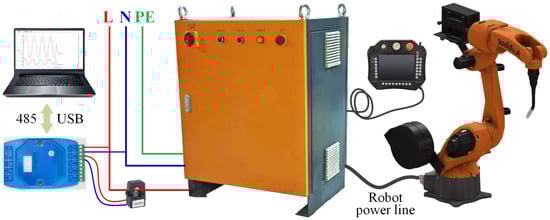
Figure 2. EC data acquisition setup for the welding robot.

To comprehensively evaluate the EC performance of the robot system under diverse motion modes, three groups of 60 points were randomly selected within the robot joint range as target points for point-to-point (PTP) joint motion. Furthermore, 10 linear paths, encompassing straight and circular motions that necessitate movement of all six robot joints, were chosen within the robot’s operational space. These linear motion paths more accurately represent the actual trajectories encountered during welding processes. Given that the welding torch mounted on the robot end-effector maintains a relatively stable load, the influence of varying loads on EC was not considered in this study. For both PTP and linear motions, the experiment utilized identical acceleration and maximum velocity parameters for the robot joints. To elucidate the EC characteristics, tests were conducted at various speeds, as delineated in Table 1.

Table 1. Robot movement velocities evaluated for EC analysis.

Movement Type	Tests Velocity
PTP/(%)	2, 5, 8, 10, 15, 20, 30, 40, 50, 70
Linear motion/(mm/s)	2, 4, 6, 8, 10, 15, 20, 30, 50, 75, 100, 150, 200, 300, 500
Circular motion/(mm/s)	2, 4, 6, 8, 10, 15, 20, 30

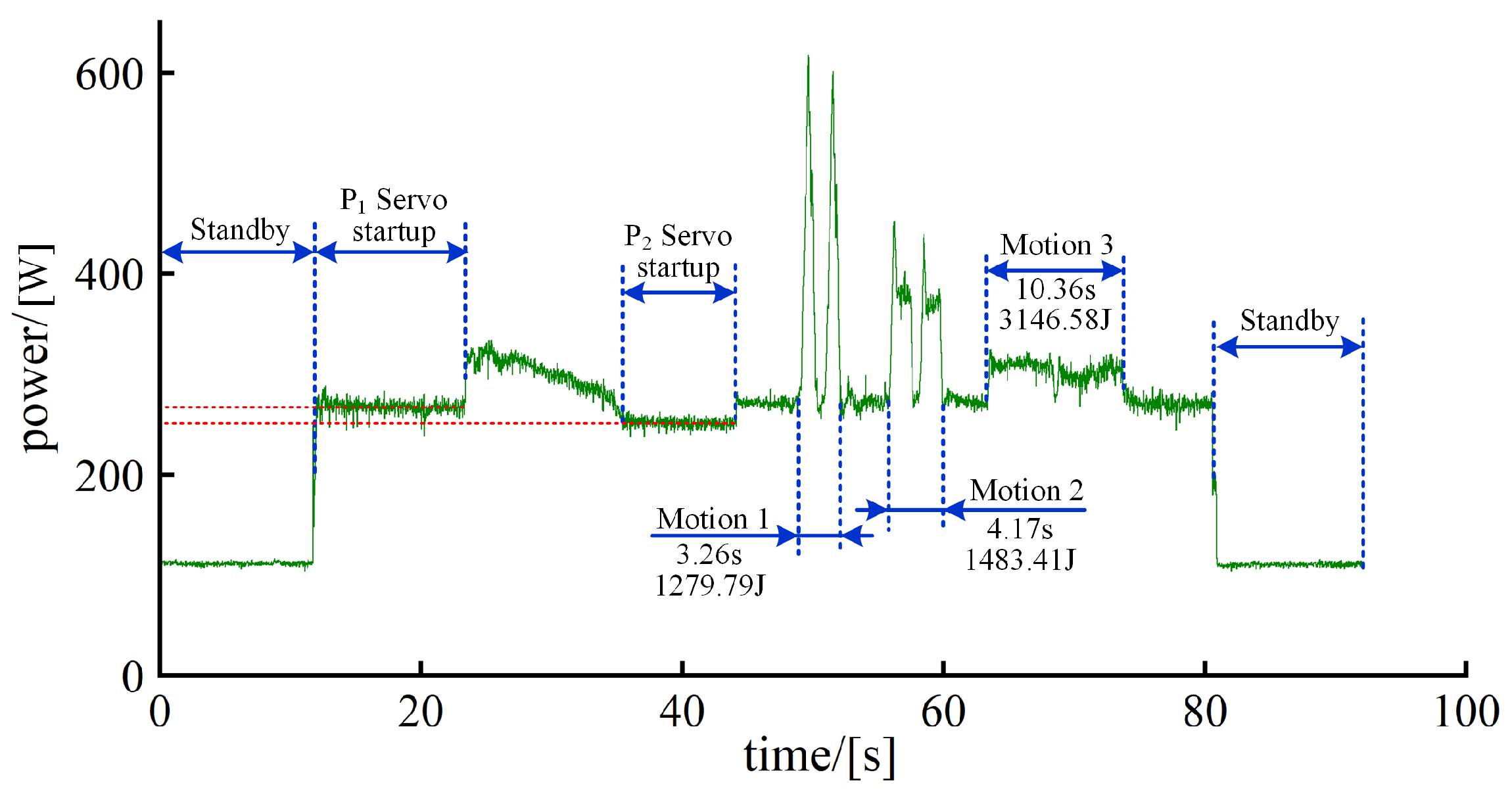
As illustrated in Figure 3, the robot EC data acquisition process comprises three distinct states: standby, servo startup, and active operation. In the standby state, the robot system is powered on, but the control system has not issued any motion commands, resulting in the robot remaining stationary. During this period, $P_a$ is solely attributed to auxiliary components, approximately 100 W. The robot transitions to the servo startup state when the control system sends a startup command to the servo drives. In this phase, the power consumption of the auxiliary components remains constant, while the mechanical arm begins to consume energy primarily for the excitation and positioning of the joint servo motors. The power consumption at this stage, minus the standby power consumption, represents the total power consumption of the joint motors $P_m$ and the losses of the servo drives $P_{s,l}$. The varying initial joint positions, exemplified by $P_1$ and $P_2$ in Figure 3, lead to different torques acting on each joint, resulting in variations in power consumption after the servo startup. Upon entering the active operation state, the robot executes the predetermined motion trajectory. Figure 3 illustrates Motion 1, Motion 2, and Motion 3, which represent the EC profiles for the same PTP path at 50%, 30%, and 10% of the maximum velocity, respectively. This comparison highlights the significant impact of operational speed on EC for a given path.

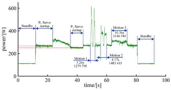
Figure 3. Analysis of EC across different robot motions.

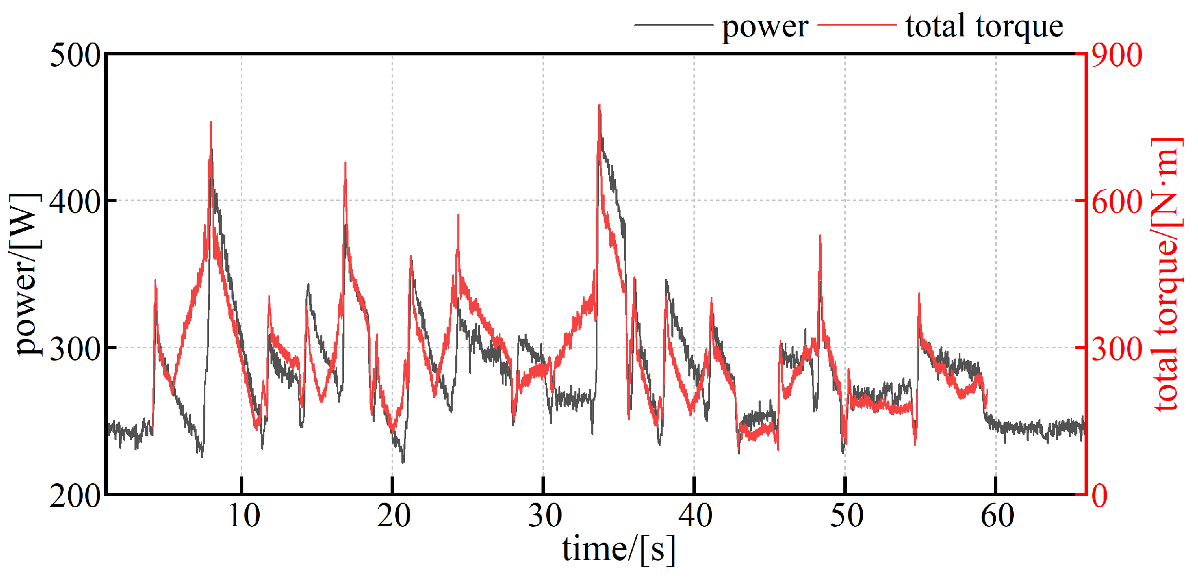
The asynchronous collection of EC and motion data during actual robot system operation necessitates data alignment. Variations in the robot system’s EC primarily result from joint motor loads. The summation of torque data from all six joints provides an intuitive representation of the overall system load at any given moment. Figure 4 illustrates the correspondence between the total torque value and the robot system’s EC. This relationship forms the basis for temporal alignment of raw EC and motion data, ensuring timestamp consistency. The alignment process yielded a dataset comprising 3,250,000 data points, each representing the robot system’s state at a specific time. These data points include EC, joint angles, joint angular velocities, joint torques, and additional variables.

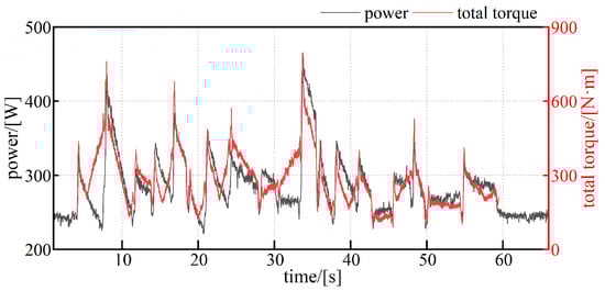
Figure 4. Correlation between robot joint torque and system EC.

2.3. Modeling Method

The complex nonlinear relationship between robot motion parameters and EC presents significant challenges in precisely identifying individual EC parameters. Consequently, this study utilizes a regression model to predict EC during robot operation. Pearson correlation coefficients (Figure 5) quantify the relationship between motion parameters and EC. The three parameters exhibiting the strongest correlation are ${\tau }_1$, ${\tau }_4$, and ${\tau }_2$. To enhance model simplicity, mitigate overfitting risk, and improve performance, the torques of all six robot joints are selected as input variables for training the regression model. Previous research by the team has explored robot dynamics, analyzing the nonlinear characteristics of joint torques in welding robots during low-velocity motion using chaos theory. The non-rigid-body dynamics component of joint torques is collectively considered, and a robot kinematic model is established by combining ordered fitting and disordered regression trees. Additionally, the phase space reconstruction method is employed to enhance the accuracy of nonlinear dynamics [27].

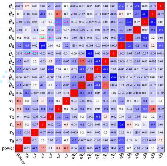
Figure 5. Pearson correlation coefficient matrix between robot motion parameters and EC.

XGBoost is an improved and optimized ensemble learning algorithm based on gradient boosting decision trees (GBDTs) [28]. It combines a series of weak classifiers, typically decision trees, also known as classification and regression trees (CARTs), into a strong classifier, achieving better prediction performance. The XGBoost model constructed in this study utilizes a dataset $D=\left\{({\mathbf{x}}_i,y_i)\right\}(i=1,2,\dots ,n)$, where ${\mathbf{x}}_i$ and $y_i$ represent the joint torques and system EC, respectively. The XGBoost model can be expressed as follows:

$${\widehat{y}}_i=\mathrm{XGB}\left(x_i\right)=\sum _{k=1}^K{f}_k\left(x_i\right),f_k\in F$$

(7)

$$F=\{f\left(x\right)={\omega }_{q\left(x\right)}\}(q:{\mathbf{R}}^p\to T,\omega \in {\mathbf{R}}^T)$$

(8)

where $x_i$ represents the input data, ${\widehat{y}}_i$ is the predicted value, k is the number of CARTs in the XGBoost model, $f_k\left(x_i\right)$ is the prediction value of the k-th tree for $x_i$, F denotes the function space of CARTs, q represents the tree structure, T is the number of leaf nodes, and each $f_k$ corresponds to an independent tree structure q and leaf weights $\omega$.

XGBoost establishes k tree structures by minimizing the regularized objective function:

$$L=\sum _{i=1}^{n}l\left(y_i,{\widehat{y}}_i\right)+\sum _{k=1}^K\Omega \left(f_k\right)$$

(9)

$$l(y_i,{\widehat{y}}_i)={(y_i-{\widehat{y}}_i)}^2$$

(10)

$$\Omega \left(f_k\right)=\gamma T+{\displaystyle \frac{1}{2}}\lambda \sum _{j=1}^T{\omega }_j^2$$

(11)

where $l\left(y_i,{\widehat{y}}_i\right)$ represents the loss function term, characterizing the error between $y_i$ and ${\widehat{y}}_i$, and the regularization term $\Omega \left(f_k\right)$ is a penalty for model complexity, which helps prevent overfitting. $\gamma$ is the penalty coefficient, and $\lambda$ is the coefficient for the L2 regularization term.

XGBoost implements training by iteratively adding trees. During the t-th iteration, the predicted value ${\widehat{y}}_i^t$ for the i-th sample can be expressed as follows:

$${\widehat{y}}_i^t={\widehat{y}}_i^{t-1}+f_t\left(x_i\right)$$

(12)

The objective function can be represented as follows:

$$L^{\left(t\right)}=\sum _{i=1}^{n}l(y_i,{\widehat{y}}_i^{(t-1)}+f_t\left(x_i\right))+\Omega \left(f_t\right)$$

(13)

By employing a second-order Taylor expansion, the above equation can be approximated as follows:

$$L^{\left(t\right)}\cong \sum _{i=1}^n\left[l(y_i,{\widehat{y}}_i^{(t-1)})+g_i{f}_t\left(x_i\right)+{\displaystyle \frac{1}{2}}{h}_i{f}_t^2\left(x_i\right)\right]+\Omega \left(f_t\right)$$

(14)

$$g_i={\partial }_{{\widehat{y}}_i^{(t-1)}}l(y_i,{\widehat{y}}_i^{(t-1)})$$

(15)

$$h_i={\partial }_{{\widehat{y}}_i^{(t-1)}}^{2}l(y_i,{\widehat{y}}_i^{(t-1)})$$

(16)

where $g_i$ and $h_i$ are the first and second derivatives of the loss function term, respectively.

Defining $I_j=\left\{i\right|q\left(x_i\right)=j\}$ as the sample set of leaf node j, after removing the constant term from the equation and expanding the regularization term, the final objective function is obtained:

$${\tilde{L}}^{\left(t\right)}\cong \sum _{j=1}^T\left[\left(\sum _{i\in {\mathit{I}}_j}{g}_i\right){\omega }_j+{\displaystyle \frac{1}{2}}\left(\sum _{i\in {\mathit{I}}_j}{h}_i+\lambda \right){\omega }_j^2\right]+\gamma T$$

(17)

To develop a predictive model for the EC of a robotic system, the dataset was segmented into training, validation, and testing subsets in an 18:1:1 ratio through random sampling. The mean squared error (MSE) cost function was employed to assess the regression models. Table 2 presents a comparative analysis of the XGBoost model’s prediction performance against other regression models. Each model utilized Bayesian optimization for hyperparameter tuning, ensuring consistency in the training and testing data. Interference and various factors resulted in a MAPE of approximately 0.5% for EC measurements of the same trajectory across two sequential runs. The XGBoost model demonstrated superior prediction accuracy, achieving a MAPE of 1.86%. It also exhibited a 26.97% improvement in mean absolute error (MAE) over the highly accurate tree regression model, underscoring its exceptional performance in EC prediction tasks. Conversely, the linear regression model underperformed on all prediction metrics, with a MAE reaching 28.68 W, suggesting a complex nonlinear relationship between the joint torques and the EC in the robotic system.

Table 2. Performance comparison of regression models in EC prediction.

Model	MSE	${\mathit{R}}^2$	MAE/(W)	MAPE
Regression Tree	0.0025	0.96	5.3021	0.0186
Linear Regression	0.0371	0.43	28.6886	0.0962
Neural Networks	0.0064	0.90	11.1324	0.0370
Regression Tree Ensemble	0.0024	0.96	6.2041	0.0211
XGBoost	0.0012	0.98	3.8723	0.0131

3. Welding Robot EC Optimization

3.1. Strategies to Reduce Robot EC

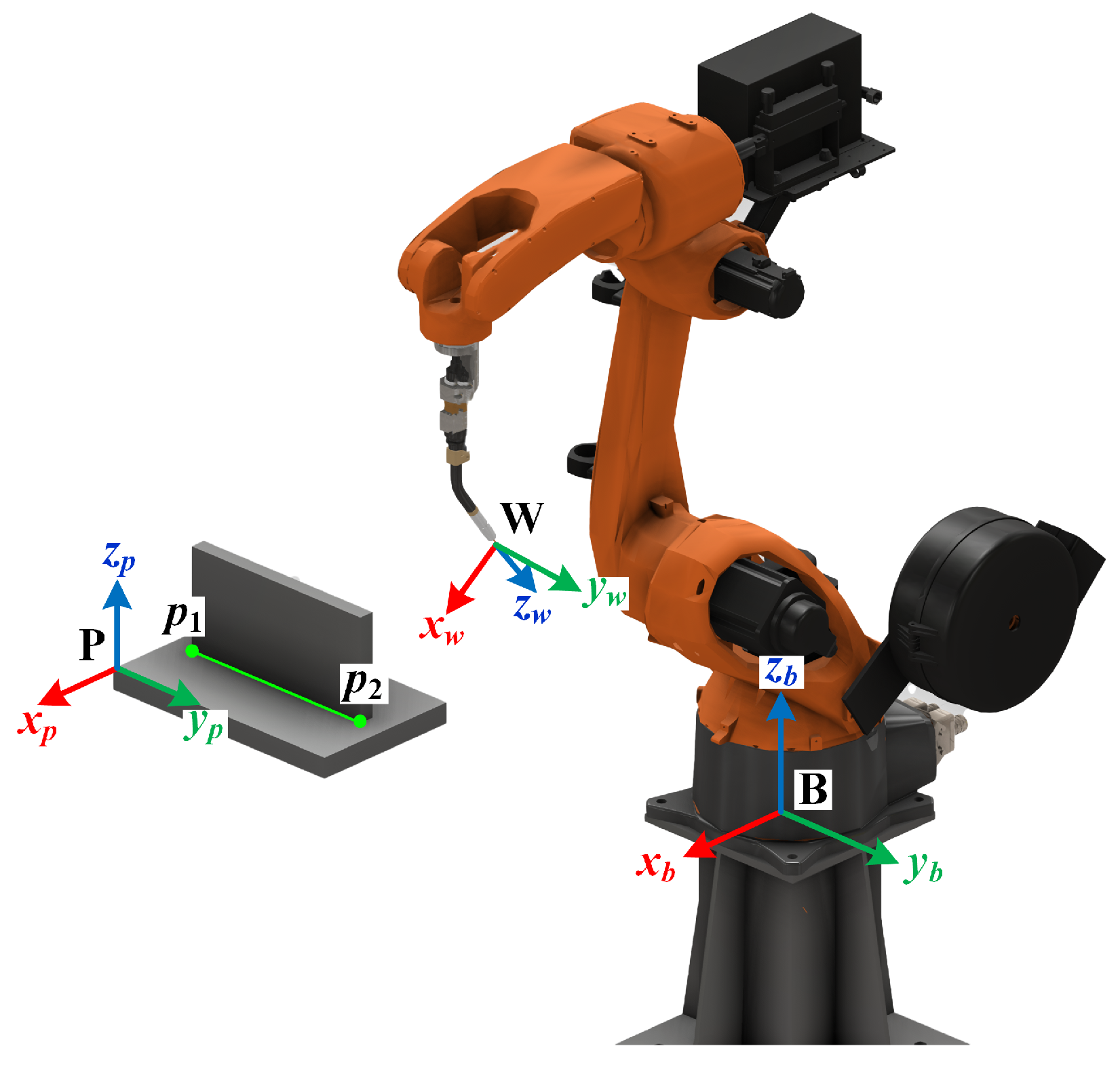
Figure 6 illustrates the coordinate transformation relationships within the welding robotic system. The transformations between the robot base coordinate system {B}, the welding torch end-effector coordinate system {W}, and the workpiece coordinate system {P} are denoted as $T_B^W$ and $T_B^P$, respectively. The welding path points $p_1$ and $p_2$ in the workpiece coordinate system are represented as $T_P^{p_1}$ and $T_P^{p_2}$. Through these transformations, we obtain the welding path points in the base coordinate system using

$$T_B^{P_1}=T_P^{P_1}{T}_B^P$$

(18)

Figure 6. Coordinate transformation relationship of welding robot system.

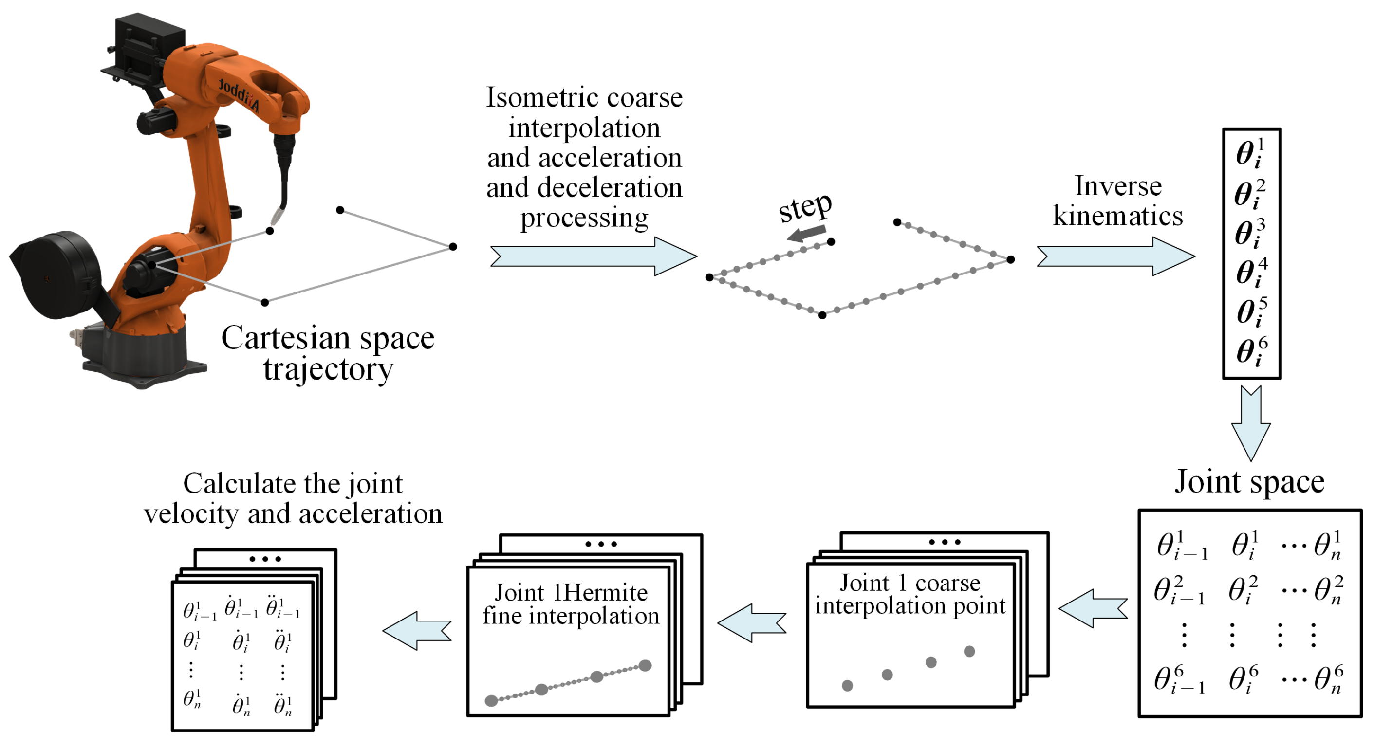
Figure 7 delineates the process of generating motion commands for the robot path. The welding trajectory undergoes Cartesian space acceleration and deceleration, as well as interpolation processing, yielding a series of end-effector points $\mathit{p}$. Through robot kinematics calculations and joint space Hermite interpolation, a sequence of joint motion parameters $(\mathit{\theta },\dot{\mathit{\theta }},\ddot{\mathit{\theta }})$ is derived. The robot controller operates in a position control mode with a 2 ms period, transmitting the desired joint positions $\mathit{\theta }$ to the servo drive system. This system incorporates cascaded control loops for position, velocity, and current, enabling precise control of motor motion to achieve the target joint positions for the robot.

Figure 7. Robot path generates motion instruction flow.

Using the precise dynamics model from our prior work [27], along with the EC prediction model developed earlier, we calculate the robot’s energy consumption:

$${\mathit{EC}}_{\mathit{robot}}=\mathit{M}.predict\left(\tau (\theta ,\dot{\theta },\ddot{\theta })\right)$$

(19)

where the robot joint torques $\tau (\theta ,\dot{\theta },\ddot{\theta })$ are calculated using Equation (2), and $\mathit{M}$ represents the EC prediction model of the robotic system.

The workpiece layout directly influences the end-effector position and orientation of the robot during the welding process, resulting in variations in joint torques and consequently affecting the EC of the robotic system. Optimizing the workpiece layout enables the robot to maintain an optimal working posture throughout the welding process, reducing energy requirements for posture adjustments and thereby lowering the EC of the welding robotic system. Using a 6 degree-of-freedom welding robot as the research subject, the optimization problem of the robotic system is mathematically defined as follows: subject to constraint conditions, determine the optimal position and orientation of the workpiece in the robot base coordinate system to minimize the EC of the robot while completing the entire welding path motion. The mathematical formulation of the optimization problem is expressed as follows:  

$$\begin{array}{c}min{E}_{robot}={\displaystyle \sum _{n=1}^N}E{C}_{robot}^{Nt}·t\\ st.\left\{\begin{array}{c}{\theta }_{min}⩽\theta ⩽{\theta }_{max}\hfill \\ \left|\dot{\theta }\right|⩽{\dot{\theta }}_{max}\hfill \\ \left|\ddot{\theta }\right|⩽{\ddot{\theta }}_{max}\hfill \\ s\left(\mathit{p}\right)\in S\hfill \end{array}\right.\end{array}$$

(20)

where $E_{robot}$ is the total EC of the robot system, N is the length of the time series, $t=2$ ms is the interpolation time, $E{C}_{robot}^{Nt}$ is the power of the robotic system at the instant $N\times t$, $({\theta }_{\min },{\theta }_{\max })$, ${\dot{\theta }}_{max}$ and ${\ddot{\theta }}_{max}$ represent the ranges of joint angles, angular velocities, and angular accelerations, respectively. S denotes the robot’s workspace, and $s\left(p\right)$ represents the welding path points in the robot coordinate system.

3.2. Optimization Method

The XGBoost model establishes a complex nonlinear mapping relationship between the EC of the robotic system and the robot joint torques, transforming the EC optimization problem into an optimization problem. Intelligent optimization algorithms with powerful search capabilities are utilized to solve this problem. The WOA proposed by Mirjalili et al. in 2016 [29], is an intelligent optimization algorithm that mathematically simulates the hunting process of whales approaching their prey. This study employs an improved whale optimization algorithm combining differential evolution (DE) and elite opposition-based learning (EOBL) to optimize the robot EC problem. The DE operator is incorporated to enhance population diversity and avoid local optima, while the EOBL strategy utilizes information from historically optimal individuals to guide the population towards the global optimum direction, improving the algorithm’s global search capability and convergence speed. To better illustrate the IWOA process, the steps of the improved whale algorithm are presented in the form of pseudocode in Algorithm 1.

The IWOA algorithm is divided into several stages as follows:

(1)

Algorithm initialization: Set the population size as $N_P$ and the maximum number of iterations as $K_{max}$.

(2)

Population initialization: Set the initial iteration step as $t=0$, and initialize the initial population using the opposition-based learning strategy.

(3)

Optimal position selection: Calculate the fitness values of the $N_P$ individuals, and select the position of the individual with the optimal fitness value as the optimal position.

(4)

EOBL: Select the top $\eta$ proportion of individuals with the best fitness values as elite individuals, and calculate their reverse solutions using the elite reverse learning strategy. Select solutions with better fitness values through competition.

(5)

Iterative calculation: Perform iterative optimization based on random search, encircling prey, and attacking prey.

(6)

DE fine-tuning: Based on the current optimal solution, perform crossover and mutation operations. If a solution with better fitness is obtained, replace the current optimal solution.

(7)

Termination condition check: If satisfied, terminate the iteration and output the current optimal solution; otherwise, return to step (3).

Algorithm 1 IWOA with DE and EOBL.

Require: Population size $N_P$, max iterations $K_{max}$, elite ratio $\eta$, DE parameters $F=0.5$,   $CR=0.9$ Ensure: Global best solution ${\mathbf{X}}_{best}$   1: Initialization:   2: Generate initial population using OBL:   3: $\mathbf{X}i=lb+ub-\mathbf{X}rand$   4: Set convergence factor $a=2$, spiral coefficient $b=1$   5: Fitness evaluation:   6: Calculate fitness for each $\mathbf{X}i$ and find $\mathbf{X}best$   7: Elite opposition-based learning:   8: Select top $\eta N_P$ elite individuals   9: For each elite ${\mathbf{X}}_e$, calculate reverse: 10: ${\mathbf{X}}_e^{reverse}=\alpha (lb+ub)-{\mathbf{X}}_e$ 11: Update ${\mathbf{X}}_e$ using greedy selection 12: while $t<K_{max}$ do 13:       Update $a=2(1-t/K_{max})$, $C=2r_1$, $p=\mathcal{U}(0,1)$ 14:       for each individual ${\mathbf{X}}_i$ do 15:             if $p<0.5$ then 16:                  Update position using encircling or global search 17:             else 18:                  Update position using bubble-net attack 19:             end if 20:       end for 21:       DE fine-tuning: 22:       Generate mutant vector: $\mathbf{V}={\mathbf{X}}_{best}+F({\mathbf{X}}_{r1}-{\mathbf{X}}_{r2})$ 23:       Perform binomial crossover and update ${\mathbf{X}}_{best}$ 24:       Cauchy mutation: 25:       Apply perturbation to ${\mathbf{X}}_{best}$ 26:       Increment iteration: $t=t+1$ 27: end while 28: Return:  ${\mathbf{X}}_{best}$

4. Experimental Results and Analysis

4.1. Experimental Platform

To validate the effectiveness of the proposed EC optimization method, experiments were conducted using a 6R welding robot, as depicted in Figure 8. The same robot was used in both the experimental setup and the EC acquisition phases, ensuring consistency in data collection. Table 3 details the robot’s technical specifications. For EC data acquisition, we employed a paperless measurement instrument that records current and voltage directly from the robot. This device is connected to a laptop via a USB interface, allowing for the synchronous acquisition and logging of electrical parameters, which are crucial for calculating the total EC using the energy model. The laptop is equipped with an Intel Core i7-1165G7 CPU and 16 GB of DDR4 RAM, capabilities that ensure the efficient processing of the EC optimization algorithms and real-time data analysis.

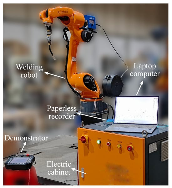
Figure 8. Welding robot experiment platform.

Table 3. Robot parameter.

Parameters	Value
Number of axes	6
Load	8 kg
Body weight	190 kg
Maximum arm span	1465 mm
Maximum power	4 kW
Repetitive positioning accuracy	±0.08 mm

4.2. Experimental Result

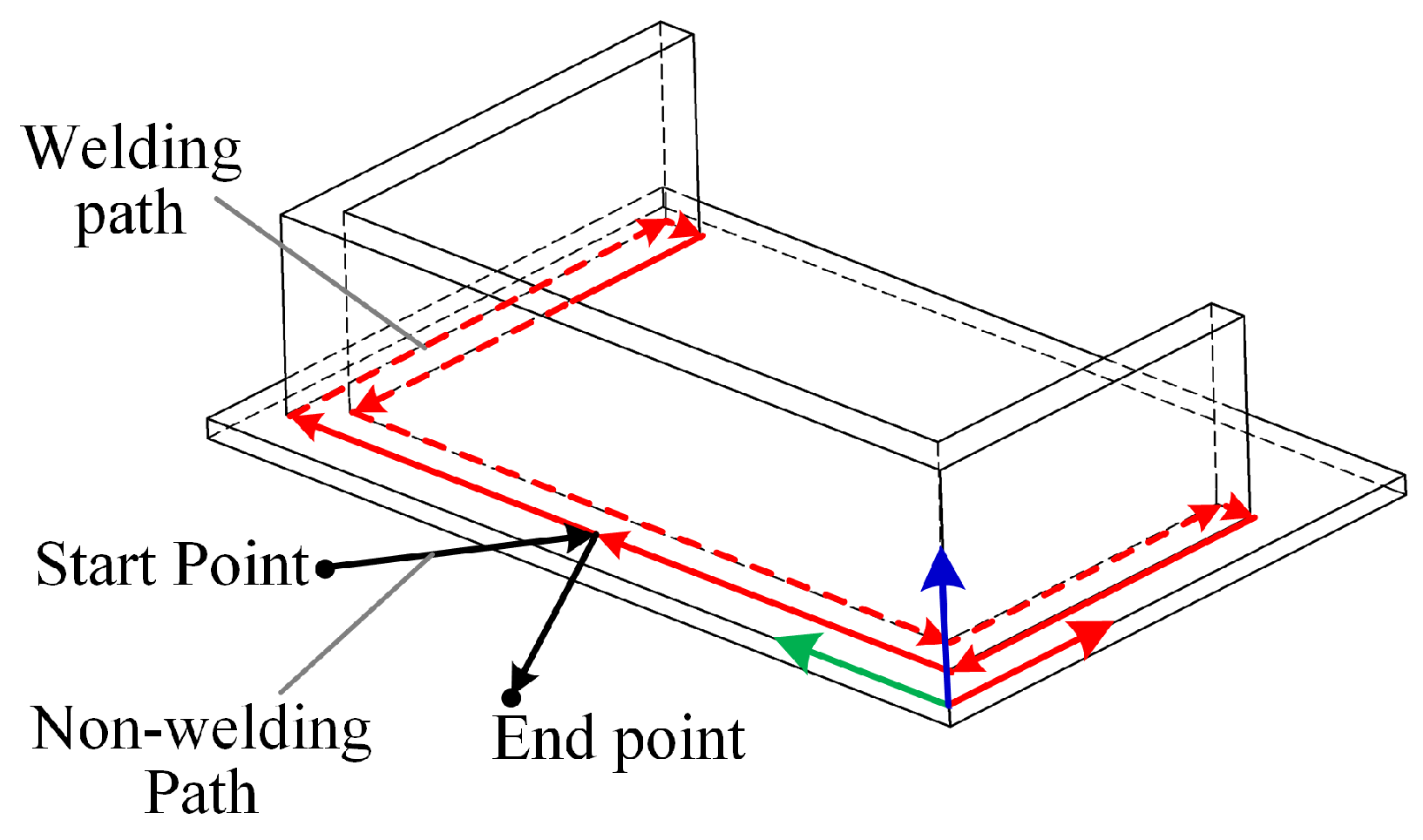
Figure 9 illustrates the workpiece used in our experiments, characterized by its trajectory that includes multiple welding and non-welding segments from the start point to the end point. To ensure weld quality, the welding path velocity is set at 10 mm/s, while the non-welding path velocity is increased to 300 mm/s to improve work efficiency. The orientation of the robot’s end-effector is determined based on the welding process to maintain the correct position and angle relative to the weld seam. Optimized parameters include the position (x, y, z) and rotation around the Z-axis (Rz) of the workpiece within the robot’s coordinate system. Considering that workpieces are typically positioned flat on the worktable in practical scenarios, rotations around the X and Y axes (Rx, Ry) are not optimized to simplify the problem and facilitate fixture design for securing the workpiece. In practical applications, the robot must adhere to constraints on joint position, velocity, and acceleration to ensure safety and controllability. The position of the workpiece coordinate system also faces specific limitations. Table 4 and Table 5 list the constraints on the position of the workpiece coordinate system and robot motion, respectively. These constraints arise from factors such as the robot’s structural parameters, workspace limitations, and requirements of the welding process for position and orientation. Incorporating these constraints into the optimization problem ensures the feasibility of the results and constrains the optimization space, thereby enhancing computational efficiency.

Figure 9. Experimental welding path for the robot.

Table 4. Robot joint motion constraints for EC optimization.

Restriction Type	Joint 1	Joint 2	Joint 3	Joint 4	Joint 5	Joint 6
Joint position/(°)	−90∼90	−45∼75	−55∼75	−85∼35	−60∼35	−300∼300
Joint velocity/(°/s)	170	420	440	860	860	1300
Joint acceleration/(°/s2)	1700	4200	3440	5840	6080	11,200

Table 5. EC optimization workpiece coordinate system position constraints.

Restriction Type	x/(mm)	y/(mm)	z/(mm)	Rz/(°)
Workpiece coordinate position	350∼1000	−800∼800	400∼1200	−90∼90

This study introduces two different optimization benchmarks for comparison: (1) Minimization of $E_{robot}$ (the proposed method): This optimization target focuses on reducing the overall energy consumption of the robotic system, making it more aligned with industrial applications and providing a more accurate prediction of energy savings during actual robot operation. (2) Minimization of $E_{motor}$: This benchmark solely minimizes the mechanical output energy consumption of joint motors, evaluating energy efficiency from the perspective of pure mechanical output. The mechanical output power of a joint motor is calculated as follows:

$$E{C}_{motor}=\sum \mathit{\tau }\left(\mathit{\theta },\dot{\mathit{\theta }},\ddot{\mathit{\theta }}\right)·\dot{\mathit{\theta }}$$

(21)

The optimization problem for the comparative method can be defined as follows:

$$\begin{array}{c}min{E}_{motor}={\displaystyle \sum _{n=1}^N}E{C}_{motor}^{Nt}·t\\ st.\left\{\begin{array}{c}{\theta }_{min}⩽\theta ⩽{\theta }_{max}\hfill \\ \left|\dot{\theta }\right|⩽{\dot{\theta }}_{max}\hfill \\ \left|\ddot{\theta }\right|⩽{\ddot{\theta }}_{max}\hfill \\ s\left(\mathit{p}\right)\in S\hfill \end{array}\right.\end{array}$$

(22)

where $E_{motor}$ is the total EC of the robot motors, $E{C}_{motor}^{Nt}$ is the power of the robotic system at the instant $N\times t$.

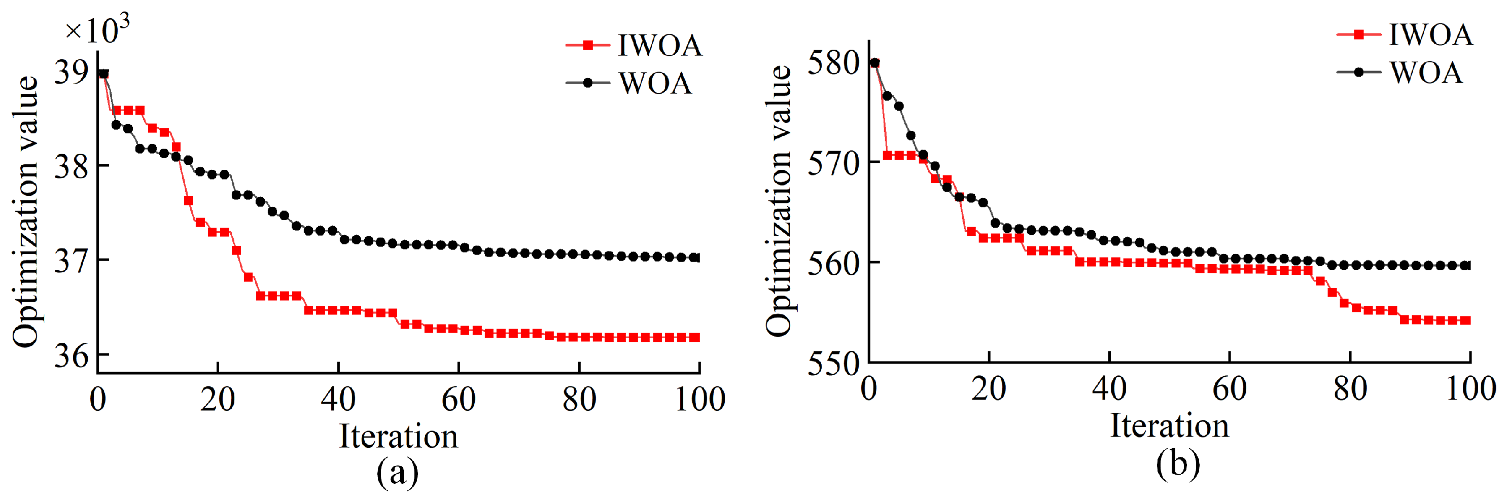
The IWOA is employed to optimize (20) and (22). The initial optimization parameters are set as follows: population size $N_p=30$, maximum iterations $K_{\max }=100$, probability parameter $p=0.3$, elite reverse learning ratio $\eta =20\%$, differential mutation factor $F=0.4$, and crossover probability $CR=0.9$. The optimization results are presented in Table 6. After applying the proposed overall robot energy consumption optimization method, the actual energy consumption of the robotic system ($E_{robot}$) is reduced by 7.17%. In contrast, the method that optimizes only the mechanical output power of the motors achieves a reduction of just 4.42% in joint motor mechanical energy consumption ($E_{motor}$). Since, during low-speed motion, the mechanical output power of the motors accounts for only a small fraction of the total system energy consumption, while non-mechanical losses (such as copper loss and iron loss within the motors, as well as friction losses in the reducers) constitute the majority of energy dissipation, there exists a significant magnitude difference between $E_{robot}$ and $E_{motor}$. This result highlights the core argument of this study: in practical applications, evaluating robotic energy consumption should not be limited to mechanical power calculations but must comprehensively account for internal losses in motors and transmission systems to accurately reflect the actual energy-saving effect of the robotic system. To further validate the improvement of the proposed IWOA over the standard WOA, the convergence curves of both algorithms for robot energy consumption optimization are compared in Figure 10. As shown in the figure, IWOA demonstrates faster convergence and achieves lower final optimization values for both $E_{robot}$ and $E_{motor}$ compared to standard WOA. This result confirms that the integration of DE and EOBL strategies effectively enhances the optimization performance of WOA in this application.

Table 6. The result of robot EC optimization.

Item	Workpiece Coordinate Position (x, y, z, Rx, Ry, Rz)	Algorithm Execution Time	Predicted ${\mathit{E}}_{\mathit{robot}}$/(J)	Predicted ${\mathit{E}}_{\mathit{motor}}$/(J)
Before optimization	(420, 450, 1150, 0, 0, 30)	-	38,965.35	579.86
Minimization of $E_{motor}$	(350.30, −659.31, 890.35, 0, 0, −55.96)	1590 s	37,020.31	554.21
Minimization of $E_{robot}$	(703.97, −161.84, 1003.01, 0, 0, −13.82)	1648 s	36,178.21	559.65

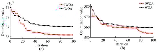
Figure 10. Convergence curves of IWOA and standard WOA for robot EC optimization: (a) $E_{robot}$; (b) $E_{motor}$.

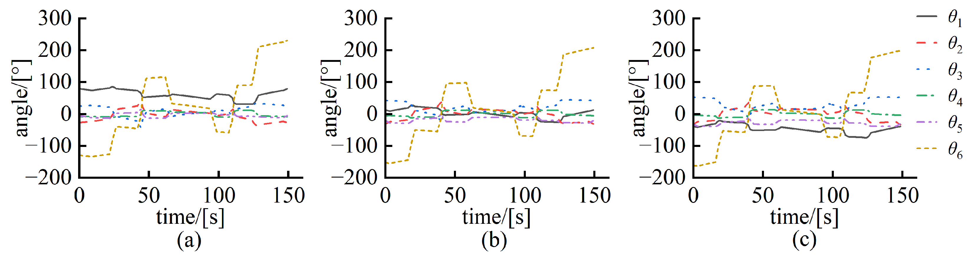
The welding path points were represented in the robot coordinate system based on the workpiece position. Using offline programming methods, robotic motion code was generated for both pre-optimization and post-optimization scenarios, allowing the controller to drive the robot along the predetermined path. As the position of the optimized workpiece coordinate system $\left\{P\right\}$ in the base coordinate system $\left\{B\right\}$ changes, the locations of the feature points along the path also adjust accordingly. Consequently, significant variations in the robot joint angles were observed (Figure 11). The absolute average values of the joint angular velocities before and after optimization are presented in Table 7. Notably, the absolute average values of the angular velocities for joints 1, 2, 3, and 6 after optimization were all reduced.

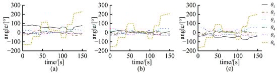
Figure 11. Comparison of robot joint positions before and after optimization: (a) original positions; (b) after optimization for minimum motor mechanical energy ($E_{motor}$); (c) after optimization of robot overall energy consumption ($E_{robot}$).

Table 7. Comparison of absolute average joint angular velocities before and after optimization.

Item	${\dot{\mathit{\theta }}}_1$/(°/s)	${\dot{\mathit{\theta }}}_2$/(°/s)	${\dot{\mathit{\theta }}}_3$/(°/s)	${\dot{\mathit{\theta }}}_4$/(°/s)	${\dot{\mathit{\theta }}}_5$/(°/s)	${\dot{\mathit{\theta }}}_6$/(°/s)
Before optimization	1.19	1.62	1.69	0.66	0.82	4.68
Minimization of $E_{motor}$	1.05	1.54	1.60	0.70	0.90	4.47
Minimization of $E_{robot}$	1.07	1.61	1.65	0.76	0.88	4.56

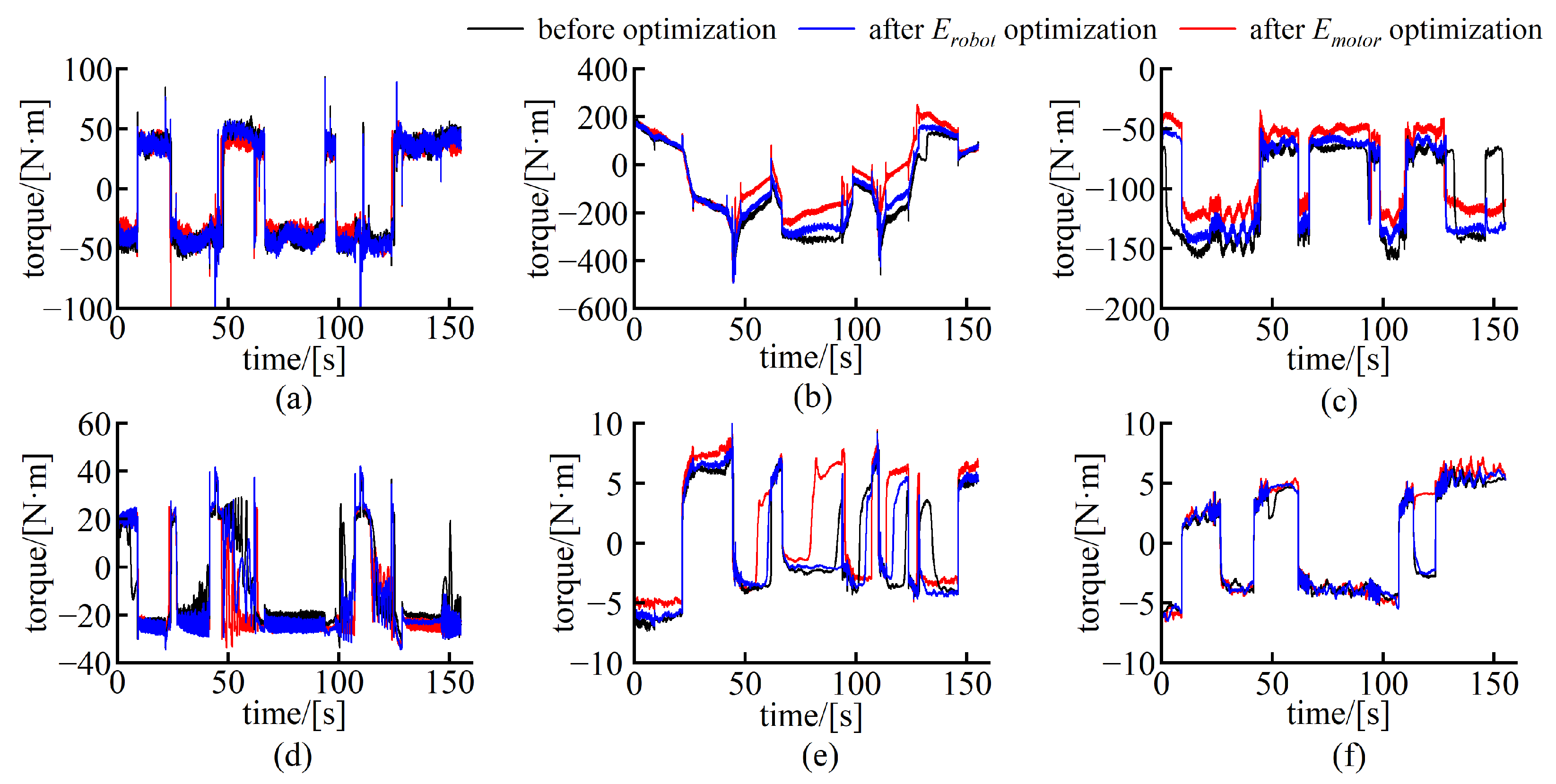
After optimizing the overall robot energy consumption using the proposed method, the kinematic parameters of each joint changed, leading to significant alterations in joint torques. Using the joint-torque profiles depicted by Figure 12 as an illustration, the pre-optimization absolute mean torques for joints were 41.69 N·m, 171.62 N·m, 103.58 N·m, 18.88 N·m, 4.20 N·m, and 3.90 N·m, respectively. After applying the proposed overall robot energy consumption optimization method, these values decreased to 40.97 N·m, 161.24 N·m, 98.62 N·m, 21.15 N·m, 4.22 N·m, and 4.04 N·m, with torques of joints 2 and 3 reduced by 6.05% and 4.79%, respectively, demonstrating the method’s significant advantage in reducing torque for high-load joints. In contrast, when using the optimization method that targets motor mechanical output power, the absolute mean values of joint torques decreased to 38.97, 131.25, 88.33, 17.72, 3.85, and 3.61 N·m, with torques of joints 2 and 3 reduced by 23.53% and 14.72%, respectively, showing a larger reduction. However, optimizing solely based on mechanical power tends to prioritize reducing the mechanical output torque itself while neglecting motor and transmission losses during actual robot operation. The energy consumption curves of the entire robot system before and after optimization are shown in Figure 13, and the statistical results are presented in Table 8. It should be noted that since the dynamic model does not fully account for friction losses in joints during actual low-speed movement, the measured EC of the robot is higher than the predicted value, resulting in a certain degree of error.

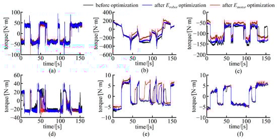
Figure 12. Comparison of joint torque curves before and after optimization. (a–f) represent joints 1–6, respectively.

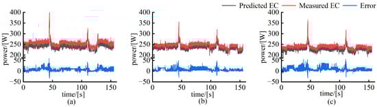
Figure 13. Comparison between predicted and measured robot system power consumption: (a) before optimization; (b) after optimization with $E_{motor}$ minimization; (c) after optimization of robot system total energy consumption ($E_{robot}$).

Table 8. Experimental validation results for actual robot energy consumption after optimization.

Item	Actual ${\mathit{E}}_{\mathit{robot}}$/(J)	Actual ${\mathit{E}}_{\mathit{motor}}$/(J)	MAE Between Predicted and Actual Power/(W)	Average Power of the ${\mathit{E}}_{\mathit{robot}}$/(W)
Before optimization	39,911.59	599.76	7.14	257.24
Minimization of $E_{motor}$	38,282.80	573.82	6.82	246.74
Minimization of $E_{robot}$	37,230.33	580.64	7.34	239.96

The proposed optimization method demonstrates high consistency between predicted and actual energy consumption. Table 8 indicates that the MAE between predicted and measured energy consumption is 7.14 W before optimization and 7.34 W after optimization, while the corresponding MAPE values are 2.50% and 2.82%. Although the prediction model slightly underestimates friction torque at low speeds, leading to predicted energy consumption generally being lower than the actual measured values, the overall error remains within a reasonable range. After applying the proposed overall robot energy consumption optimization method, the actual total energy consumption of the robotic system is reduced by 6.72%, closely aligning with the predicted reduction of 6.99% (Table 8). In contrast, the optimization method that targets motor mechanical output power achieves a 4.33% reduction in actual motor mechanical energy consumption during testing, which is higher than the 3.19% reduction achieved by the proposed method. However, in terms of the total actual energy consumption of the robotic system, the proposed method achieves a 6.72% reduction, significantly outperforming the mechanical output power optimization method, which only results in a 4.08% reduction. These results further validate the effectiveness of the proposed method. By comprehensively considering both mechanical power and non-mechanical losses in the motor and transmission system, the proposed approach more accurately reduces the actual energy consumption of the overall robotic system. By optimizing the position and posture of the workpiece, the method not only decreases motor mechanical energy consumption but also significantly reduces the overall energy losses during actual robot operation, making it more suitable for practical industrial applications.

5. Conclusions

This study presents a data-driven modeling and trajectory optimization approach to address energy-saving issues in welding robot systems. By analyzing the components of a typical arc welding robot system, an XGBoost regression model has been established to predict system EC based on self-measured energy data, achieving a MAPE of 1.86%. The trajectory planning problem was formulated as an optimization task, and an IWOA has been employed to solve it. By adjusting the position of the workpiece coordinate system in the robot coordinate frame (x, y, z) and rotating around the Z-axis (Rz), the robot’s motion trajectory was optimized while adhering to physical constraints such as joint position, velocity, and acceleration limits. Experimental results demonstrated that the optimized robot system’s predicted EC decreased by 6.99%, while the actual EC reduced by 6.72%. These findings validate the effectiveness of the EC optimization method proposed in this research when compared to the method for minimizing joint motor EC. The discrepancies between the predictive model and actual outcomes provide valuable insights for future model improvements and algorithm optimizations.

This research applies data-driven methods to EC modeling and optimization in robotic systems, demonstrating the feasibility and effectiveness of this approach through experiments. Compared to traditional physics-based models, the data-driven method better captures the complex characteristics of robotic systems, improving the accuracy of EC predictions. The IWOA effectively reduces the robot system’s EC while satisfying various physical constraints in solving the trajectory planning problem. The study enriches the methodologies for EC modeling and optimization in robotic systems, offering new insights for further improving energy efficiency. The proposed method can accurately estimate and reduce EC in welding robot systems, contributing to lower production costs and increased efficiency, with broad application prospects. Future work will focus on improving prediction accuracy by incorporating more features and optimizing model structures, as well as exploring more efficient trajectory optimization algorithms to further reduce EC in welding robots.

References

- Wang, B.; Hu, S.J.; Sun, L.; Freiheit, T. Intelligent welding system technologies: State-of-the-art review and perspectives. J. Manuf. Syst. 2020, 56, 373–391. [Google Scholar] [CrossRef]
- Yu, H.; Peng, Z.; He, Z.; Huang, C. Application maturity evaluation of building steel structure welding robotic technology based on multi-level gray theory. Eng. Constr. Archit. Manag. 2023, 31, 4372–4397. [Google Scholar] [CrossRef]
- Wang, X.; Xia, Z.; Zhou, X.; Guo, Y.; Gu, X.; Yan, H. Multiobjective path optimization for arc welding robot based on DMOEA/D-ET algorithm and proxy model. IEEE Trans. Instrum. Meas. 2021, 70, 1–13. [Google Scholar] [CrossRef]
- Xiao, W.; Han, G.; Ally, A.S.; Chen, X. Energy consumption modeling and parameter identification based on system decomposition of welding robots. Int. J. Adv. Manuf. Technol. 2024, 130, 1579–1594. [Google Scholar] [CrossRef]
- Pellicciari, M.; Avotins, A.; Bengtsson, K.; Berselli, G.; Bey, N.; Lennartson, B.; Meike, D. AREUS—Innovative hardware and software for sustainable industrial robotics. In Proceedings of the 2015 IEEE International Conference on Automation Science and Engineering (CASE), Gothenburg, Sweden, 24–28 August 2015; pp. 1325–1332. [Google Scholar] [CrossRef]
- Rubio, F.; Llopis-Albert, C.; Valero, F.; Besa, A.J. Sustainability and optimization in the automotive sector for adaptation to government vehicle pollutant emission regulations. J. Bus. Res. 2020, 112, 561–566. [Google Scholar] [CrossRef]
- Yao, M.; Zhou, X.; Shao, Z.; Wang, L. A general energy modeling network for serial industrial robots integrating physical mechanism priors. Robot. Comput.-Integr. Manuf. 2024, 89, 102761. [Google Scholar] [CrossRef]
- Vergnano, A.; Thorstensson, C.; Lennartson, B.; Falkman, P.; Pellicciari, M.; Leali, F.; Biller, S. Modeling and optimization of energy consumption in cooperative multi-robot systems. IEEE Trans. Autom. Sci. Eng. 2012, 9, 423–428. [Google Scholar] [CrossRef]
- Liu, A.; Liu, H.; Yao, B.; Xu, W.; Yang, M. Energy consumption modeling of industrial robot based on simulated power data and parameter identification. Adv. Mech. Eng. 2018, 10, 1687814018773852. [Google Scholar] [CrossRef]
- Meike, D.; Pellicciari, M.; Berselli, G. Energy efficient use of multirobot production lines in the automotive industry: Detailed system modeling and optimization. IEEE Trans. Autom. Sci. Eng. 2013, 11, 798–809. [Google Scholar] [CrossRef]
- Zhou, J.; Yi, H.; Cao, H.; Jiang, P.; Zhang, C.; Ge, W. Structural decomposition-based energy consumption modeling of robot laser processing systems and energy-efficient analysis. Robot. Comput.-Integr. Manuf. 2022, 76, 102327. [Google Scholar] [CrossRef]
- Li, X.; Lan, Y.; Jiang, P.; Cao, H.; Zhou, J. An efficient computation for energy optimization of robot trajectory. IEEE Trans. Ind. Electron. 2021, 69, 11436–11446. [Google Scholar] [CrossRef]
- Heredia, J.; Schlette, C.; Kjærgaard, M.B. Data-driven energy estimation of individual instructions in user-defined robot programs for collaborative robots. IEEE Robot. Autom. Lett. 2021, 6, 6836–6843. [Google Scholar] [CrossRef]
- Yao, M.; Zhao, Q.; Shao, Z.; Zhao, Y. Research on power modeling of the industrial robot based on ResNet. In Proceedings of the 2022 7th International Conference on Automation, Control and Robotics Engineering (CACRE), Xi’an, China, 14–16 July 2022; pp. 87–92. [Google Scholar] [CrossRef]
- Zhang, M.; Yan, J. A data-driven method for optimizing the energy consumption of industrial robots. J. Clean. Prod. 2021, 285, 124862. [Google Scholar] [CrossRef]
- Yan, J.; Zhang, M. A transfer-learning based energy consumption modeling method for industrial robots. J. Clean. Prod. 2021, 325, 129299. [Google Scholar] [CrossRef]
- Jiang, P.; Wang, Z.; Li, X.; Wang, X.V.; Yang, B.; Zheng, J. Energy consumption prediction and optimization of industrial robots based on LSTM. J. Manuf. Syst. 2023, 70, 137–148. [Google Scholar] [CrossRef]
- Lin, H.I.; Mandal, R.; Wibowo, F.S. BN-LSTM-based energy consumption modeling approach for an industrial robot manipulator. Robot. Comput.-Integr. Manuf. 2024, 85, 102629. [Google Scholar] [CrossRef]
- Gadaleta, M.; Pellicciari, M.; Berselli, G. Optimization of the energy consumption of industrial robots for automatic code generation. Robot. Comput.-Integr. Manuf. 2019, 57, 452–464. [Google Scholar] [CrossRef]
- Soori, M.; Arezoo, B.; Dastres, R. Optimization of energy consumption in industrial robots, a review. Cogn. Robot. 2023, 3, 142–157. [Google Scholar] [CrossRef]
- Luo, X.; Li, S.; Liu, S.; Liu, G. An optimal trajectory planning method for path tracking of industrial robots. Robotica 2019, 37, 502–520. [Google Scholar] [CrossRef]
- Li, Y.; Wang, Z.; Yang, H.; Zhang, H.; Wei, Y. Energy-optimal planning of robot trajectory based on dynamics. Arab. J. Sci. Eng. 2023, 48, 3523–3536. [Google Scholar] [CrossRef]
- Gadaleta, M.; Berselli, G.; Pellicciari, M.; Sposato, M. A simulation tool for computing energy optimal motion parameters of industrial robots. Procedia Manuf. 2017, 11, 319–328. [Google Scholar] [CrossRef]
- Wang, X.; Yan, Y.; Gu, X. Spot welding robot path planning using intelligent algorithm. J. Manuf. Process. 2019, 42, 1–10. [Google Scholar] [CrossRef]
- Mitra, A.; Bhowmik, S.; Chowdhury, S. V/f Control of PMSM Drive fed from PR Current Controller Based Single-Phase AFE Rectifier. In Proceedings of the 2024 IEEE 3rd International Conference on Control, Instrumentation, Energy & Communication (CIEC), Kolkata, India, 25–27 January 2024; pp. 337–342. [Google Scholar] [CrossRef]
- Garcia, R.R.; Bittencourt, A.C.; Villani, E. Relevant factors for the energy consumption of industrial robots. J. Braz. Soc. Mech. Sci. Eng. 2018, 40, 1–15. [Google Scholar] [CrossRef]
- Jia, B.; Chen, L.; Zhang, L.; Fu, Y.; Zhang, Q.; Pan, H. Vibration suppression of welding robot based on chaos-regression tree dynamic model. Nonlinear Dyn. 2024, 112, 4393–4407. [Google Scholar] [CrossRef]
- Sheng, C.; Yu, H. An optimized prediction algorithm based on XGBoost. In Proceedings of the 2022 International Conference on Networking and Network Applications (NaNA), Urumqi, China, 3–5 December 2022; pp. 1–6. [Google Scholar] [CrossRef]
- Mirjalili, S.; Lewis, A. The whale optimization algorithm. Adv. Eng. Softw. 2016, 95, 51–67. [Google Scholar] [CrossRef]
Disclaimer/Publisher’s Note: The statements, opinions and data contained in all publications are solely those of the individual author(s) and contributor(s) and not of MDPI and/or the editor(s). MDPI and/or the editor(s) disclaim responsibility for any injury to people or property resulting from any ideas, methods, instructions or products referred to in the content. |
© 2025 by the authors. Licensee MDPI, Basel, Switzerland. This article is an open access article distributed under the terms and conditions of the Creative Commons Attribution (CC BY) license (https://creativecommons.org/licenses/by/4.0/).