Abstract
Fault diagnosis is one of the most important issues for a modular multilevel converter (MMC). However, conventional solutions are deficient in two aspects. Firstly, they lack the necessary feature information. Secondly, they are incapable of performing open-circuit fault diagnosis of the modular multilevel converter with the requisite degree of accuracy. To solve this problem, an intelligent diagnosis method is proposed to integrate the modal time–frequency diagram and FFT-CNN-BiGRU-Attention. By selecting the phase current and bridge arm voltage as the core fault parameters, the particle swarm algorithm is used to optimize the Variational Modal Decomposition parameters, and the fault signal is decomposed and reconstructed into sensitive feature components. The reconstructed signals are further transformed into modal time–frequency diagrams via continuous wavelet transform to fully retain the time–frequency domain features. In the model construction stage, the frequency–domain features are first extracted using the fast Fourier transform (FFT), and the local patterns are captured through a combination with a convolutional neural network; subsequently, the timing correlations are analyzed using bidirectional gated loop cells, and the Attention Mechanism is introduced to strengthen the key features. Simulations show that the proposed method achieves 98.63% accuracy in locating faulty insulated gate bipolar transistors (IGBTs) in the sub-module, with second-level real-time response capability. Compared with the recently published scheme, it maintains stable performance under complex working conditions such as noise interference and data imbalances, showing stronger robustness and practical value. This study provides a new idea for the intelligent operation and maintenance of power electronic devices, which can be extended to the fault diagnosis of other power equipment in the future.
1. Introduction
With the rapid development of renewable energy, flexible direct current transmission technology (VSC-HVDC) has been widely used in offshore wind power and long-distance transmission due to its high efficiency and flexibility [1]. The modular multilevel converter (MMC), as the core equipment of the system, has the advantages of low harmonics, high efficiency, and high reliability. Nevertheless, the intricate nature of VSC-HVDC introduces novel challenges, particularly in the realm of submodule fault detection and diagnosis. Sub-module open-circuit faults can lead to output voltage distortion and open-circuit bridge arm current abnormality and even trigger system downtime, which seriously affects the stable operation of power systems [2].
Open-circuit faults are characterized in the following ways:
1. Abnormal voltage: When an open circuit fault occurs in a submodule, it can lead to an imbalance in voltage between modules, resulting in abnormal system voltage fluctuations. This voltage fluctuation is an important feature in diagnosing an open circuit fault of MMC.
2. Abnormal current: The circuit is broken due to an open circuit fault, which makes the current unable to flow, resulting in a significant decrease in the output current of the module or no output current.
3. Increase in heat: An open circuit fault causes an increase in the internal resistance of the module, which in turn causes an increase in heat, which can be observed in the infrared thermogram and is an effective means of troubleshooting.
4. Frequency response changes: Using time–frequency analysis methods, changes in the frequency response of the system during a fault can be observed, especially an increase in harmonic components, which is important for early fault diagnosis.
By comprehensively analyzing the above fault characteristics, a more comprehensive fault diagnostic model can be established to improve the accuracy and speed of identifying open-circuit faults submodules. These features can not only provide a basis for fault localization but also provide important reference information for subsequent fault recovery and maintenance. Therefore, an in-depth study of the open-circuit failure characteristics of MMC submodules is of great significance to improve the application range and reliability of MMC technology.
Existing submodule fault diagnosis methods mainly include two categories based on signal analysis and machine learning. Signal-analysis-based methods identify faults by detecting changes in voltage and current waveforms, but they are sensitive to noise and difficult to accurately distinguish fault types. Machine learning-based methods achieve fault classification by training models, but they rely on a large amount of labeled data and have limited performance when dealing with complex nonlinear signals. In addition, the existing methods still need to be improved in terms of real-time and robustness. In recent years, MMC submodule fault diagnosis techniques have received extensive attention.
Signal-analysis-based methods identify faults by detecting changes in voltage and current waveforms. For example, a wavelet-transform-based fault diagnosis method was proposed to detect open-circuit faults by analyzing the high-frequency components of submodule voltages [3]. Another interesting method was proposed in [4] to use the Hilbert–Huang transform (HHT) to extract the time–frequency characteristics of signals to achieve accurate fault localization. However, such methods are sensitive to noise and have limited performance in dealing with complex nonlinear signals.
Machine-learning-based methods achieve fault classification by training models. For example, the support vector machine (SVM) was proposed in [5] to classify submodule faults. In [6], the convolutional neural network (CNN) was used to extract fault features. Although these methods improve the diagnostic accuracy to some extent, they rely on a large amount of labeled data and perform poorly when dealing with concurrent multi-fault scenarios.
Deep learning methods show significant advantages in fault diagnosis. For example, the Long Short-Term Memory Network (fault diagnosis model) was used in [7] to capture the long-term dependencies of temporal signals. the LSTM was applied in [8] to enhance the representation of key features. However, there is still room for improvement in the comprehensiveness of feature extraction and model generalization ability of existing methods by combining the Attention Mechanism.
In summary, existing methods are deficient in terms of noise robustness, feature extraction capability, and generalization performance.
The fault diagnosis method proposed in this study based on a modal time–frequency diagram aims to overcome these limitations and, for FFT-CNN-BIGRU-Attention, provide an efficient and reliable solution to the open circuit fault diagnosis of MMC submodules.
2. MMC Fault Characterization and Selection of Characteristic Variables
MMC is the core equipment of a flexible DC transmission system, characterized by high efficiency, low harmonics, and high reliability [9]. The basic structure consists of the MMC three-phase bridge arms, and each arm contains two sub-module groups (Upper Arm and Lower Arm), and each sub-module group consists of several sub-modules (Submodule, SM) connected in series. The sub-module is the smallest functional unit, for which the MMC usually adopts a half-bridge or full-bridge structure, and its core components include the IGBT, diode, and DC capacitor. The working principle is to control the input and removal of the sub-module, to regulate the amplitude and phase of the output voltage, and to realize the conversion of DC and AC power [10]. During operation, the capacitors of the submodules maintain the stability of the DC voltage by charging and discharging, while the switching action of the MMC determines the waveform of the output voltage. the IGBTs modular design not only improves the voltage level and power capacity of the system but also enhances the redundancy and reliability of the system [11].
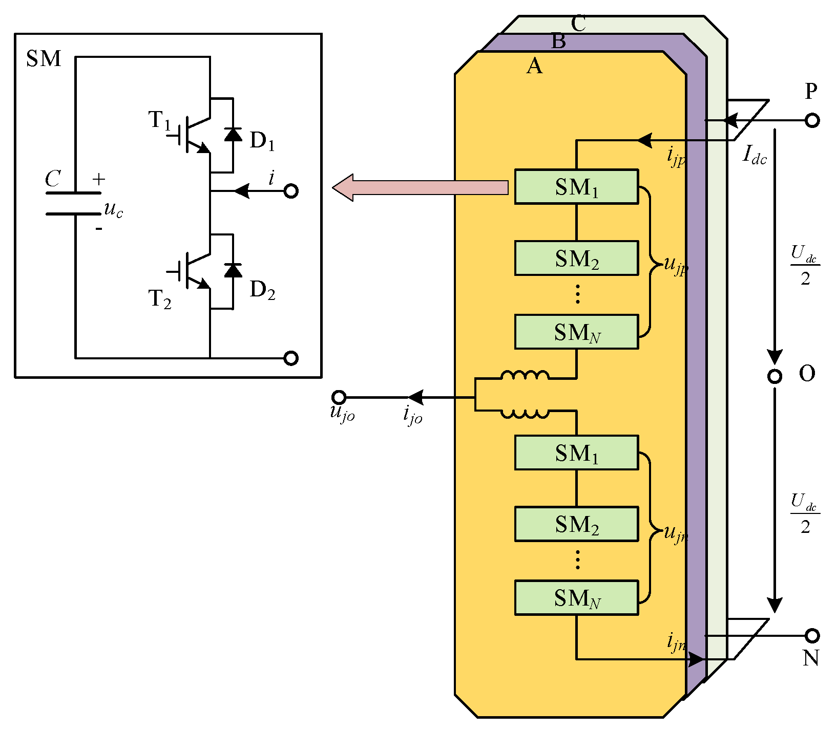
The most prevalent three-phase MMC topology in the power industry is shown in Figure 1. Each phase of the MMC consists of upper and lower bridge arms N sub-modules connected in series, and two reactors are connected in series to suppress the interphase circulating currents. ujo and ijo, (j = A, B, C) are the output phase voltage and phase current of the AC side, respectively. The middle of the upper and lower arms ujo and ijo, (j = A, B, C) are the output phase voltages and phase currents on the AC side, respectively; L is the value of the bridge arm reactance; Udc is the voltage on the DC side; Idc is the current on the DC side; Ujp and Ujn are the voltages on the upper and lower bridge arms, respectively; ijp and ijn are the currents on the upper and lower bridge arms, respectively. The upper left shows the half-bridge submodule structure, where T1 and T2 are the IGBTs in the submodule, and uc is the submodule capacitance voltage.
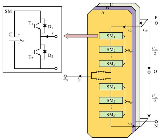
Figure 1.
MMC circuit schematic.
The normal operating modes of the submodule are the input mode and excision mode. When T1 is on and T2 is off, the submodule is in the input mode; at this time, the submodule output voltage U is equal to the submodule capacitance voltage Uc. When T1 is off and T2 is on, the submodule is in the resection mode; at this time, U is equal to 0 V. In order to accurately represent the submodule operating state, the submodule switching function Si is defined as
Based on Equation (1), the submodule output voltage relationship can be expressed as U and the capacitor voltage as Uc
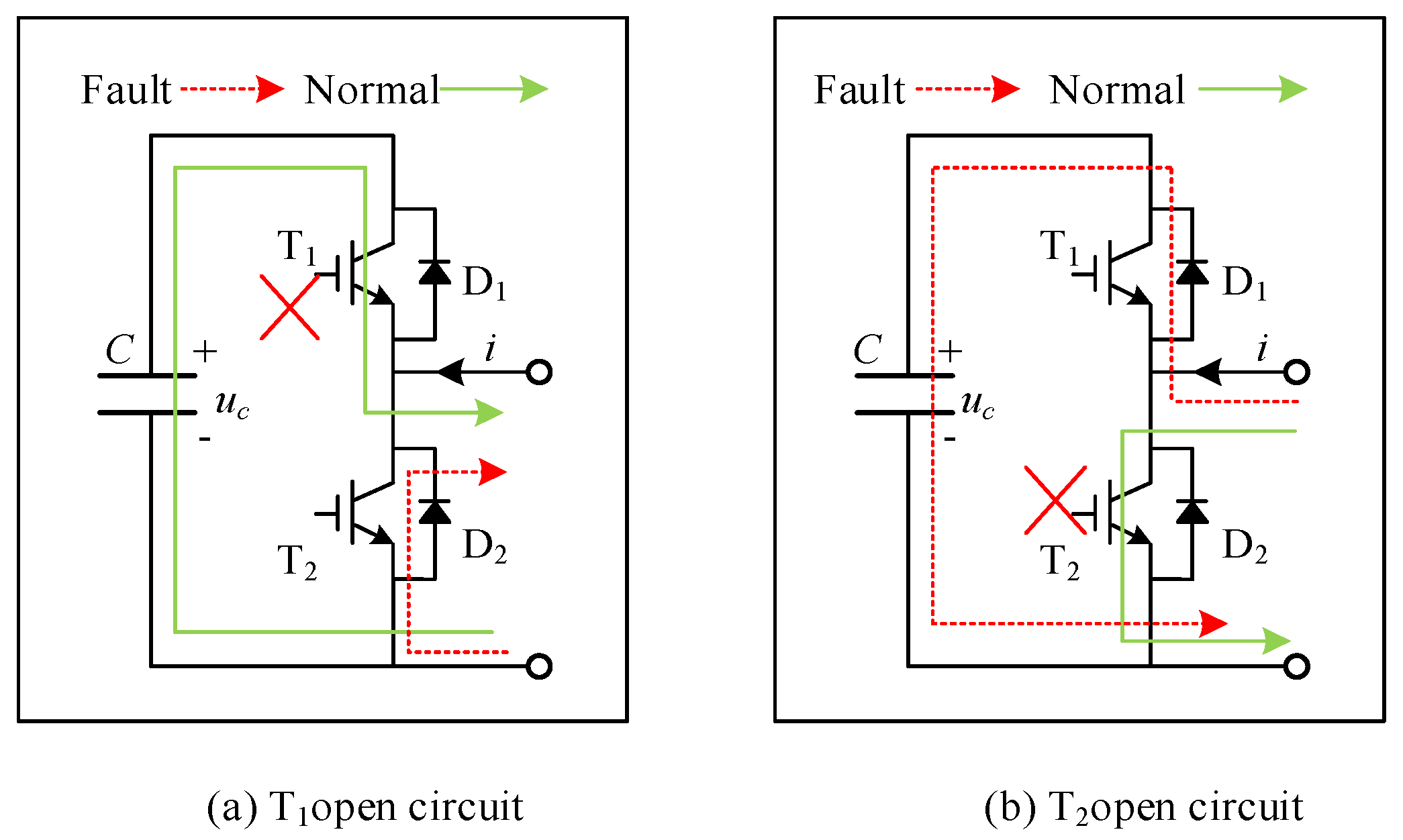
When Si = 1 and i > 0 (the direction of current flow into the submodule is specified to be positive), the bridge arm current in i flows into capacitor C through diode D1; at this time, the capacitor is in the charging mode, and the capacitor voltage is increasing. When Si = 0 and i > 0, i flows through T2, and the current path is shown in the figure; at this time, the capacitor C is bypassed and the capacitor voltage remains constant. When Si = 1 and i < 0, the current path is shown in Figure 2, and i flows from capacitor C through T1; at this time, the capacitor is in the discharging mode, and the capacitor voltage keeps decreasing. When Si = 0 and i < 0, the capacitor voltage remains constant.
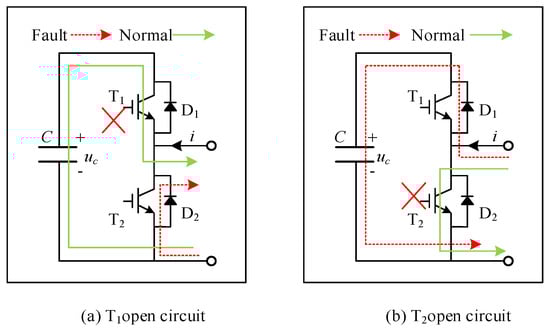
Figure 2.
IGBT open circuit fault diagram.
When a submodule open-circuit fault occurs, the current cannot pass through the faulty T1 or T2 IGBT, so the current path through the submodule is changed compared with the normal submodule. Therefore, Equation (2) cannot accurately describe the output voltage and capacitance current of the faulty submodule. The current path and capacitor voltage fault characteristics of the faulty submodule need to be reanalyzed in the case of an open-circuit fault in the IGBT.
After an open-circuit fault occurs in an IGBT, all faults will be different from the normal Vce, which can be considered to be chosen as an index for fault detection and localization. By using normalized electrical signal deviations as fault quantification indicators and comparing them with the set open circuit fault threshold of 10%, when ΔVce > 0.1ΔVce_normal, the fault flag is triggered. The number of sub-modules is too many, and using MMC Uc alone as a fault characteristic parameter will lead to too much data, especially when utilizing the deep learning model, which will produce problems such as a dimensional catastrophe. Therefore, there is a need to find the parameter that is not too computationally intensive and reflects the feature in question in order to reduce the amount of computation.
When the open-circuit fault occurs in the lower bridge arm of the phase, the three-phase current situation of the jth is just opposite to that of the upper bridge arm of the phase, i.e., in different phases of the jth when the open-circuit fault occurs, the output three-phase current can be used for the diagnosis of the faulty bridge arm, and according to the rule of change of the three-phase current, it can be localized to the specific faulty bridge arm; in the process of work, the voltage of the bridge arm of the submodules is related to the switching state of each submodule, and the switching state of each submodule is affected by the MMC modulation strategy The switching state of each submodule is affected by the MMC modulation strategy. Under the carrier-phase shift control, the switching timing signals of the submodules are fixed, and when a submodule fails, the bridge arm voltage data brought by different faulty submodules are different, and the data characteristics corresponding to the fault of each submodule will not change. That is, the bridge arm voltage can be used for faulty submodules under the carrier-phase-shift-control strategy for the localization of IGBTs In summary, the three-phase currents and bridge arm voltages are selected for diagnosing the faulty bridge arm and locating the fault in the submodule fault characterization variables for IGBT.
3. FFT-CNN-BIGRU-Attention Modal Time–Frequency Diagram Based on Fault Diagnosis Method
3.1. Particle Swarm Algorithm with VMD Decomposition
The Particle Swarm Optimization (PSO) algorithm stems from the bionics study of avian foraging behavior. This algorithm initiates with the random initialization of a particle swarm, where each particle serves as a feasible solution to the optimization problem. The fitness value of each particle is evaluated according to the objective function. Particles navigate toward the current global optimal particle, and the optimal solution is derived through iterative generational searches. There are two extreme values in each generation of the population, one is the optimal solution best found by the particle itself, and the other is the one found by the whole population. There are two optimal solutions for P (best optimal solution best extreme values in each generation of the population; one is the particle itself, and the other is the found by the whole population) [12]. After finding these two extreme values, the particle updates its speed and position according to the following formula.
where Vid represents the velocity of the i particle in the d dimension; ω is the inertia weight, which is a non-negative number; c1 and c2 are nonnegative constants. Pid and Pgd are the individual optimal value and global optimal value of the corresponding dimensions. Xid is the individual observation value of the corresponding dimension.
By iteratively updating the speed and position, the particles gradually approach the optimal solution. The PSO algorithm is simple, efficient, and easy to implement and is widely used in the fields of function optimization, parameter tuning, and so on.
Variational Mode Decomposition (VMD) is a state-of-the-art signal decomposition method that can adaptively decompose a complex signal into multiple eigenmode functions. The core idea is to decompose a signal into modal components with specific center frequencies and bandwidths by solving a variational problem. VMD constructs a constrained optimization problem to a signal decomposed into f(t) K modal functions uk(t), each with a center frequency and finite bandwidth. The objective is to minimize the sum of the bandwidths of all modal functions while ensuring that the sum of the modal functions is equal to the original signal.
The constraints are as follows:
Among them, is the modal function, and is the center frequency of each modal.
The modal functions and center frequencies are iteratively updated until convergence using the alternating direction multiplier method ADMM.
Since the open-circuit faults are many and similar in characteristics, it is difficult to diagnose the faults empirically. With the help of MMCs in the VMD algorithm, the complex signals are decomposed into components at different scales for MMCs and IMF to filter out the components that contain the most fault information and the strongest impact components, IMF, so that the modal time–frequency diagrams can be converted to contain the main fault components.
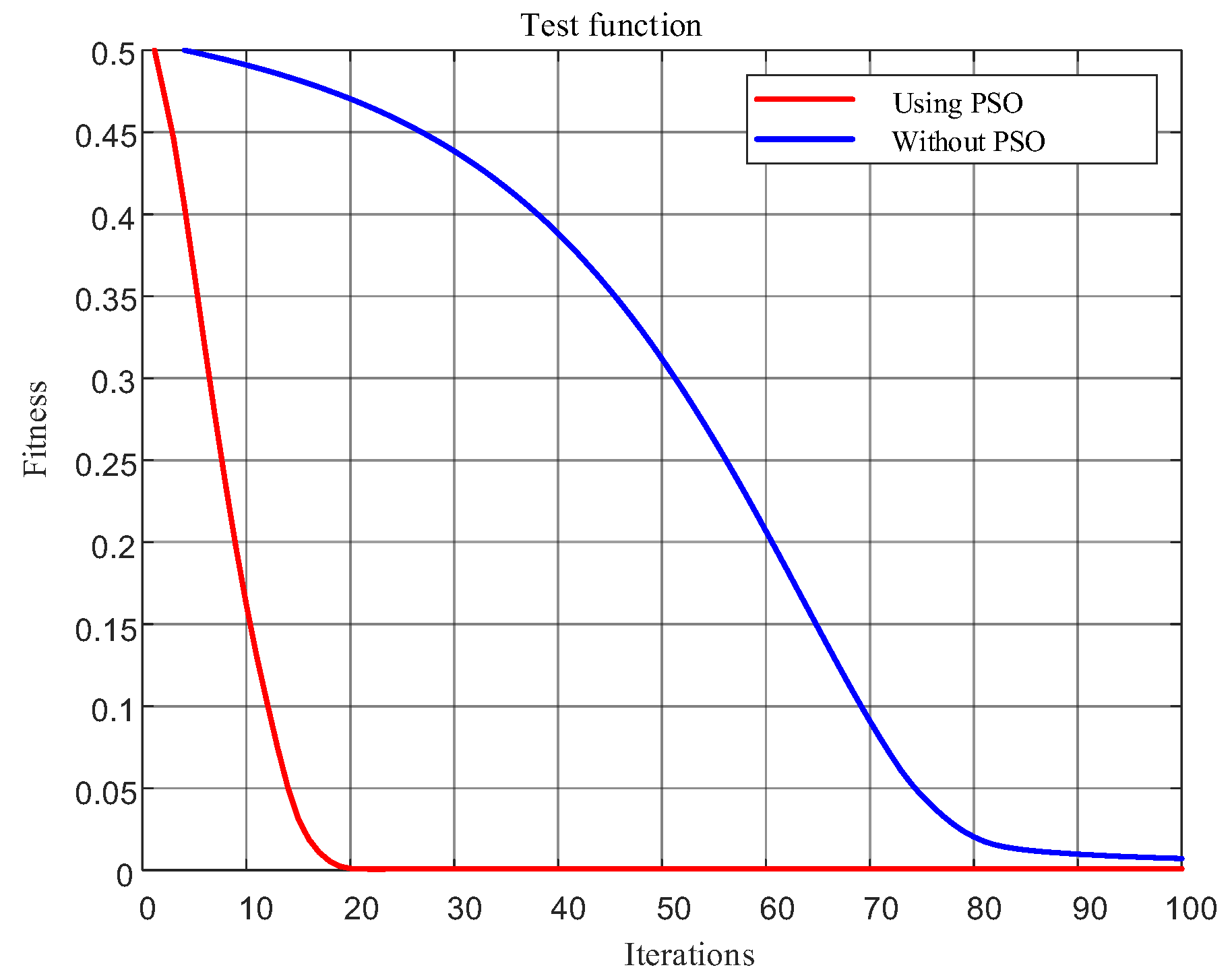
In order to verify the superiority of the particle swarm algorithm proposed in this paper, the particle swarm algorithm and the traditional one, using the same test function, the VMD decomposition algorithm, are tested. In the test set, the population number of the algorithm is 50, the iteration parameter is 100, and the fitness function is the minimum sample entropy, and each algorithm for different test functions are 10 times to find the optimal test; a test of the two algorithms in different test function convergence curves is shown in Figure 3.
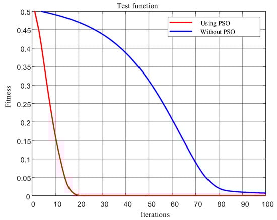
Figure 3.
Convergence curve of particle swarm algorithm.
3.2. Fast Fourier Transform
Fast Fourier Transform (FFT) is an algorithm for the efficient computation of the Discrete Fourier Transform (DFT) and its inverse transform. When dealing with large datasets, its efficiency far exceeds the direct application of the DFT. The FFT algorithm reduces the time complexity of the DFT from O(n2) by decomposing it to O, which significantly improves the speed of the computation. This algorithm has a wide range of applications in various fields, such as signal processing, pattern recognition, and communication systems.
In this study, the FFT algorithm was mainly used to analyze the MMC submodule open-circuit fault signal in the frequency domain. By performing the FFT transform on the fault signal, the time-series signal can be converted into a frequency–domain signal, which facilitates the identification and extraction of the frequency features associated with the fault. This transformation makes it possible to analyze the fault mechanism and diagnosis because faults usually produce significant changes in the frequency range [13].
The core of the FFT algorithm lies in the factorization of the decomposition basis matrix and the iterative computation using the rotational property of complex numbers. This iterative process can be realized by recursive or partitioning strategies, using smaller DFT subproblems at each step to simplify the computation. For a DFT of size N, if the Radix-2 algorithm is used, only N/2 multiplications are required to complete the computation, which greatly improves the efficiency of the algorithm.
The applicability of FFT is not limited to simple single DFT operations but can be extended to variants such as multipoint DFT (MDFT), inverse MDFT, and so on, in order to adapt to the needs in different application scenarios. In current power electronic systems, especially in MMC sub-modules, the FFT method has become an important tool in fault diagnosis due to its powerful functions and high efficiency. The FFT algorithm provides important technical support for the open-circuit fault diagnosis of MMC sub-modules by providing a fast means of frequency analysis.
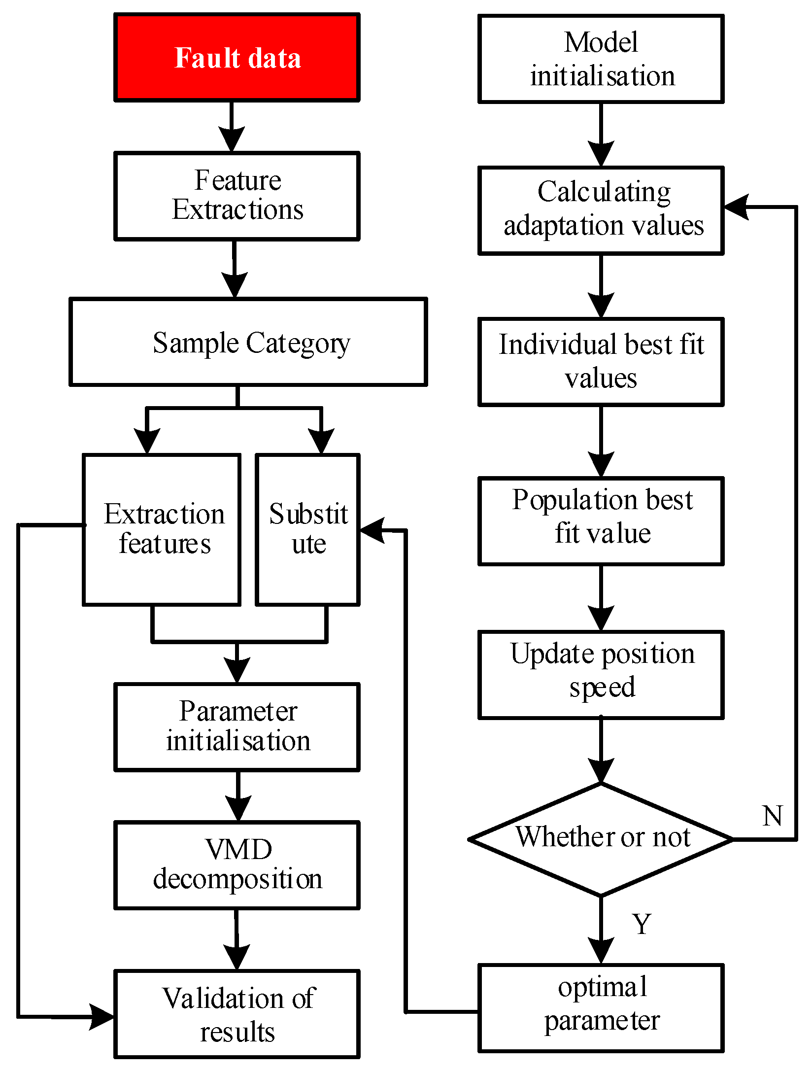
Variational Modal Decomposition is used to analyze the system signal hierarchically. After obtaining the set of intrinsic modal functions through multi-scale modal decomposition, the modal component IMF carrying significant fault characteristics and the transient response is selected as the key object of analysis, and then, the time–frequency feature map with the preservation of main features is constructed, which provides high information density input samples for the subsequent artificial intelligence diagnosis. And the specific steps of optimizing VMD using PSO algorithm are as follows:
First, simulate and acquire current signals under fault conditions, and perform preliminary data processing on the sampled signals to obtain samples. Initialize PSO parameters, including the population size N, maximum iteration count nmax, inertia weight ω, individual learning factor c1, and population learning factor c2. Perform VMD modal decomposition on the fault current signals, with initial settings including the sampling frequency Fs, upper and lower limits of the number of modal decompositions K, the upper and lower limits of the penalty factor α, and the convergence tolerance. The Kth component with the minimum arrangement entropy is calculated and iterated, and the position of the individual particle is obtained. In the particle swarm algorithm, the particle position and velocity are updated, and the process is iterated until the termination condition is met. The optimal number of modal decompositions K and penalty factor α are obtained, along with all IMF components after VMD decomposition. The processed components are reconstructed, and the denoised signal is obtained. The flowchart is shown in Figure 4.

Figure 4.
PSO-VMD program framework.
3.3. CNN Networks
A Convolutional Neural Network (CNN) is a deep learning architecture that is widely used in pattern recognition and data classification problems due to its excellent performance in the field of image recognition. CNN processes the input data through a structure that contains convolutional, pooling, and fully-connected layers, where the convolutional fully-connected layer maps the features obtained from the layer and is responsible for extracting the features in the input data, and the pooling layer is used to reduce the dimensionality of the features and increase the model’s generalization ability and the intermediate processing to the output space. The fully connected layer maps the features obtained from the intermediate processing to the output space.
In this study, CNN networks are applied to fault-diagnosis models, mainly utilizing their ability in learning and extracting valuable features from large amounts of data. By designing appropriate convolutional kernel and convolutional layer parameters, the CNN was able to automatically extract key fault features from the MMC submodule open-circuit fault data. These features were then used to train other layers of neural network models for accurate fault diagnosis.
The application of CNNs in fault diagnosis models mainly includes the following aspects: first, data preprocessing, which improves the quality of input data through techniques such as normalization or standardization; second, feature extraction, where CNNs are able to automatically discover useful fault features from the original signals; and third, feature selection, which enhances the model’s feature selection capability by adding multiple convolutional and pooling layers to improve the accuracy of fault diagnosis. The CNN is used in conjunction BIGRU-Attention in order to achieve better fault diagnosis performance.
3.4. BIGRU Network
BIGRU (Bidirectional Gated Recurrent Unit) is a special recurrent neural network structure that combines forward and backward information flow. Compared with unidirectional RNN, BIGRU can better capture long distance dependencies in sequence data. the diagnosis of open-circuit faults in the MMC submodules network is used to efficiently extract fault features and perform fault identification in BIGRU.
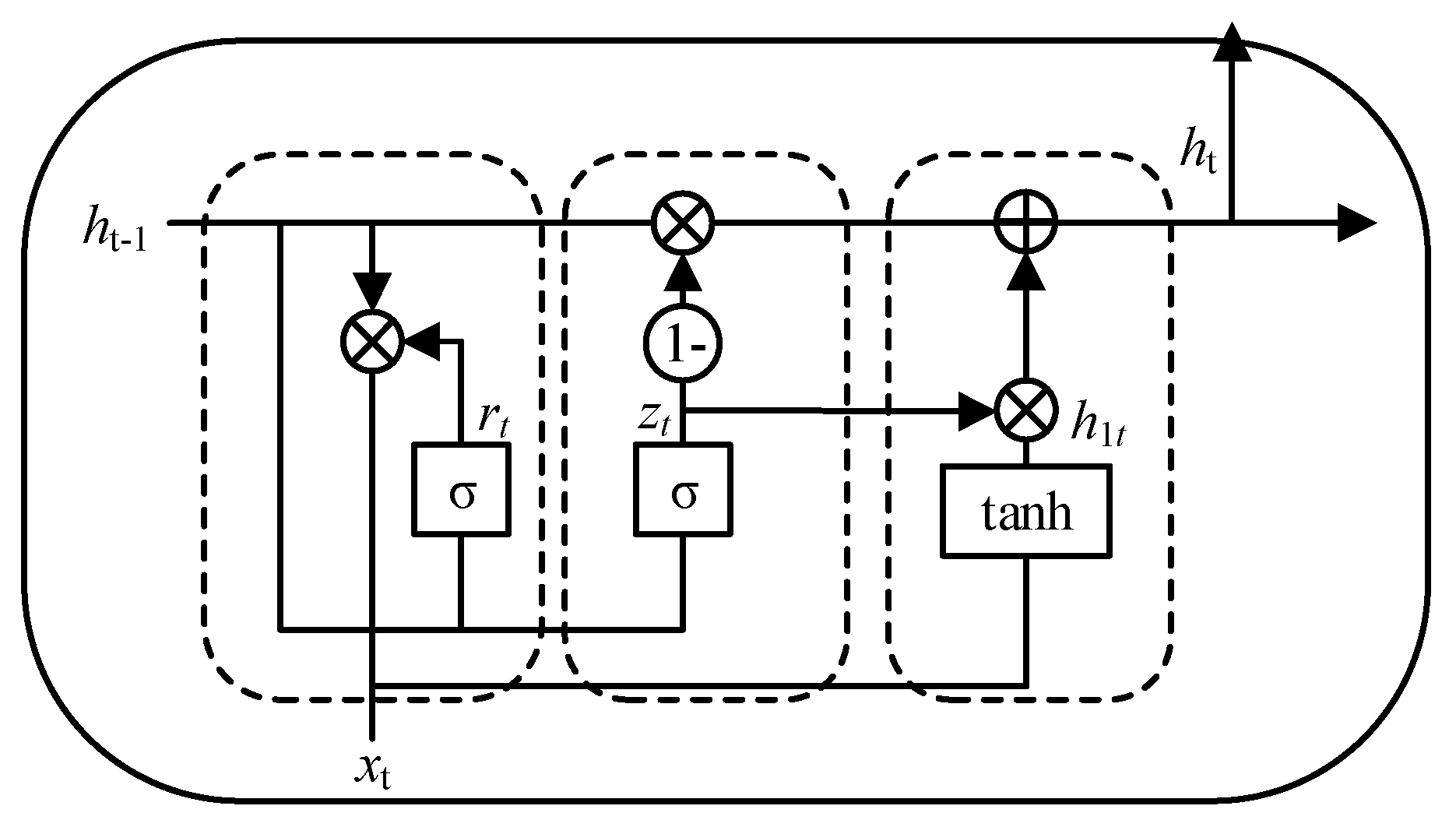
BIGRU networks control the flow of information by introducing two gates in each cell: a forgetting gate and an input gate. Unlike traditional GRUs, BIGRUs have a bi-directional propagation mechanism within the network, which means that the network not only takes into account the information at the current moment in the time series, but also is able to take into account the information at all previous moments. This bi-directional flow of information makes BIGRU perform particularly well in handling tasks that require the utilization of contextual information. The structure of the GRU is shown below in Figure 5:

Figure 5.
GRU schematic.
When the GRU uses the input at moment xt and the output at the previous moment ht−1 as input, there is
Where , , , , , , , and , are the weight matrix and bias vector of the neural network; and are the activation functions. rt represents the reset gate, and zt represents the update gate. The smaller the value of rt, the smaller the matrix value obtained by multiplying it with ht−1 and the smaller the value obtained by multiplying it with the weight matrix. In other words, the smaller the value of , the more things need to be forgotten and discarded in the previous moment.
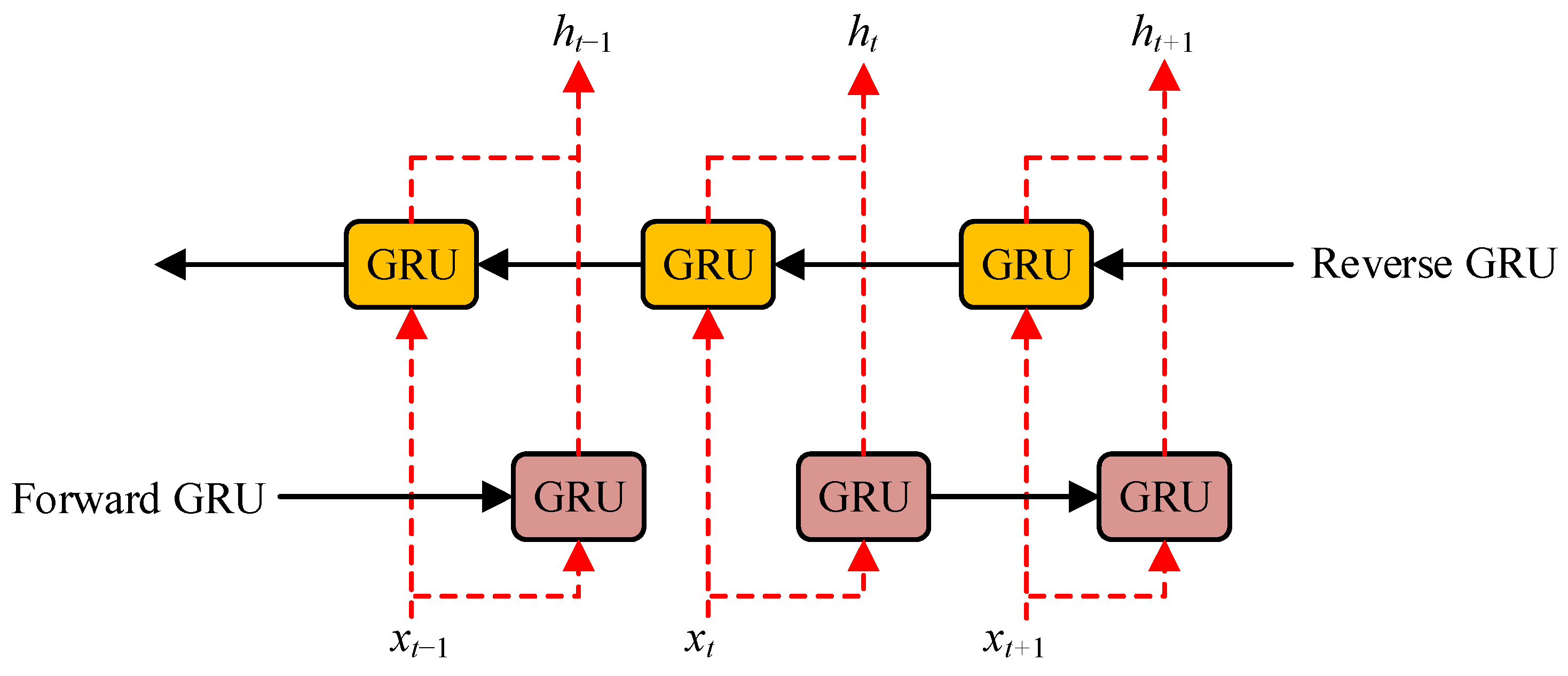
The basic structure of BIGRU is shown in Figure 6. In Figure 6, BiGRU consists of two GRU units in opposite directions, both of which play the roles of capturing past time series information and future time series information, respectively. The results of the captured information are finally outputted and merged in position according to the corresponding dimensions to enhance the prediction accuracy of the overall model.
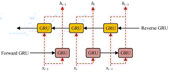
Figure 6.
BiGRU schematic.
In the fault diagnostic model, BIGRU works by the following:
1. First, a sequence of inputs is fed into BIGRU units, and each BIGRU unit first uses a forgetting gate to determine whether the information from the previous moment should be forgotten.
2. The current state is then updated according to the decision of the forgetting gate and the proportion of new information is determined by the input gate.
3. Finally, the network integrates the states from the forward and reverse hidden layers to generate the final output for fault identification.
Due to its excellent performance, BIGRU has been widely used in the field of net-work fault diagnosis. In this study, the BIGRU network was used as the core part of the fault diagnosis model with a view of achieving more accurate and faster fault identification. By learning and analyzing the time series features of fault signals, BIGRU can effectively identify different types of fault patterns, thus improving the efficiency and accuracy of fault diagnosis.
3.5. Attention Mechanism
The Attention Mechanism is a key technique in the field of machine learning that can improve the performance of a model, and it has especially demonstrated its power in processing sequence data. In this study, the Attention Mechanism is introduced to the FFT-CNN-BIGRU-Attention fault diagnosis model to enhance the model’s ability to recognize the open-circuit fault features of MMC submodules.
The core of the Attention Mechanism is its ability to focus on the most important parts of the input sequence, thus enhancing the model’s perception of critical information. In our model, this mechanism is used to emphasize those time-frequency diagram features that are more important for fault diagnosis. In this way, the model is able to identify and analyze fault-related features more accurately, thereby improving the accuracy and efficiency of fault diagnosis.
In the specific implementation, the Attention Mechanism adopts the Multi-Head Self-Attention (MHSA) network structure. This structure is able to view the input features from different perspectives at the same time and capture different patterns and relationships in the input sequence through multiple parallel attention heads. This parallel processing capability greatly enriches the model’s ability to capture input features and enables the model to show higher flexibility and adaptability when facing complex and multiple fault signals.
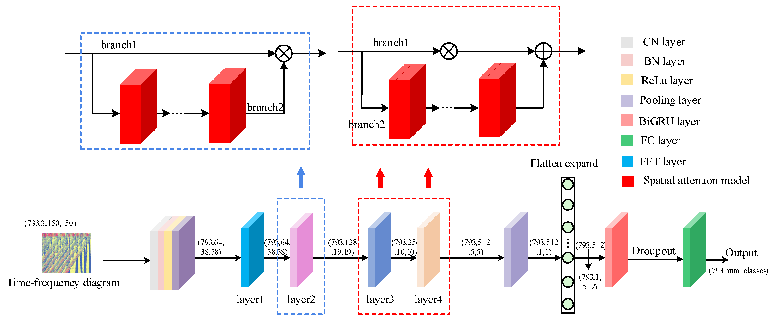
To concretely implement this process, we first convert the modal time–frequency map into sequence data. Then, the BIGRU network structure is utilized to obtain the time-dependent information of the sequence data. At this stage, each time step is regarded as an independent unit to be processed by the model, which helps the model to capture the temporal order and contextual information in the input sequence. Finally, the Attention Mechanism is introduced to further enhance the model’s sensitivity to important features within a particular time step. In this way, the model is able to detect the MMC sub more accurately and identify the specific cause of fault generation in an open-circuit fault module. The constituted FFT-CNN-BIGRU-Attention structure is shown in Figure 7.
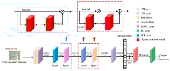
Figure 7.
Basic structure of FFT-CNN-BIGRU-Attention.
3.6. Troubleshooting Process
The fault diagnosis process is based on the constructed FFT-CNN-BIGRU-Attention, aiming to accurately identify open-circuit faults in the MMC submodule. The model combines the FFT algorithm to extract the fundamental frequency components of the signal, the CNN network to capture the local features, the BIGRU network to process the sequence data, and the Attention Mechanism to reinforce the key information to form a comprehensive fault diagnosis system. FFT is a crucial step in this process, as it converts the original time-domain signal into a frequency-domain representation. This conversion is instrumental in capturing frequency-dependent features in the signal that are critical for effective fault diagnosis. Subsequently, a Convolutional Neural Network is applied to the time–frequency map. The CNN’s convolution kernel is adept at capturing locally relevant patterns, processing the entire local region in parallel, and facilitating more efficient and intuitive feature extraction. This approach is advantageous in terms of hierarchical feature extraction. According to the CNN model, a high-level localized feature sequence is first extracted. Subsequently, the BiGRU model is employed to process this sequence. The BiGRU model integrates information from both the forward GRU and backward GRU, with the objective of comprehensively modeling long-distance backward and forward dependencies throughout the entire sequence. The Attention Mechanism is implemented based on the output of the Bidirectional Gated Recurrent Unit, which learns a weight distribution. The BiGRU dynamically determines the importance of the features in the sequence at different time steps and assigns weights and sums accordingly. The combination of these mechanisms results in a well-designed, cascading feature extraction and comprehension process. This combination achieves an optimal balance between computational efficiency and model expressiveness, demonstrating superior performance in comparison to numerous single models or combination schemes that are inadequately complementary.
(1) The five-level MMC is selected as the diagnostic target based on the diagnostic approach. Seven bridge arm operating states are simulated, including six fault conditions and one normal state. Phase currents are sampled under the different fault conditions and used as raw signals. These raw signals are then used to diagnose bridge arm faults. Next, the faulty bridge arm is selected as the diagnostic target. Using the experimental platform, we simulate the bridge arm voltage U(j) and the phase currents of the nine IGBT submodules under operational conditions, including eight submodule fault states and one normal state. Then, the IGBTs are located through sampling. The bridge arm voltage under the IGBT fault conditions Uj and phase current ij are sampled, which are used as the raw signals to locate the faulty IGBT.
(2) The phase current ij and bridge arm voltage Uj are normalized, and under different fault categories, the phase current ij and bridge arm voltage Uj are partitioned into samples by a sliding window feature extraction algorithm to obtain raw current sample 1 and raw voltage sample 2.
(3) PSO-VMD processing is performed on the raw current and voltage sample data collected in step (2) to extract a series of sensitive and high-quality IMF components. These IMF components are reconstructed, and the reconstructed signals are used as inputs for the continuous wavelet transform (CWT) to generate modal time–frequency maps. After preprocessing the modal time–frequency maps, faulty bridge arm diagnosis dataset 1 and the faulty IGBT localization dataset 2 are constructed, respectively, and the dataset 1 and dataset 2 are randomly divided into the training set, validation set, and test set to ensure that the three datasets do not overlap with each other. The training set is used to input into the FFT-CNN-BIGRU-Attention model with set parameters for training. After each round of training, the validation set is used to optimize and validate the model to ensure that the model training process is continuously optimized during and the performance and is continuously improved. If the validation results are not satisfactory, the model hyperparameters are adjusted. When the training reaches the set number of iterations, the trained model is saved for subsequent testing.
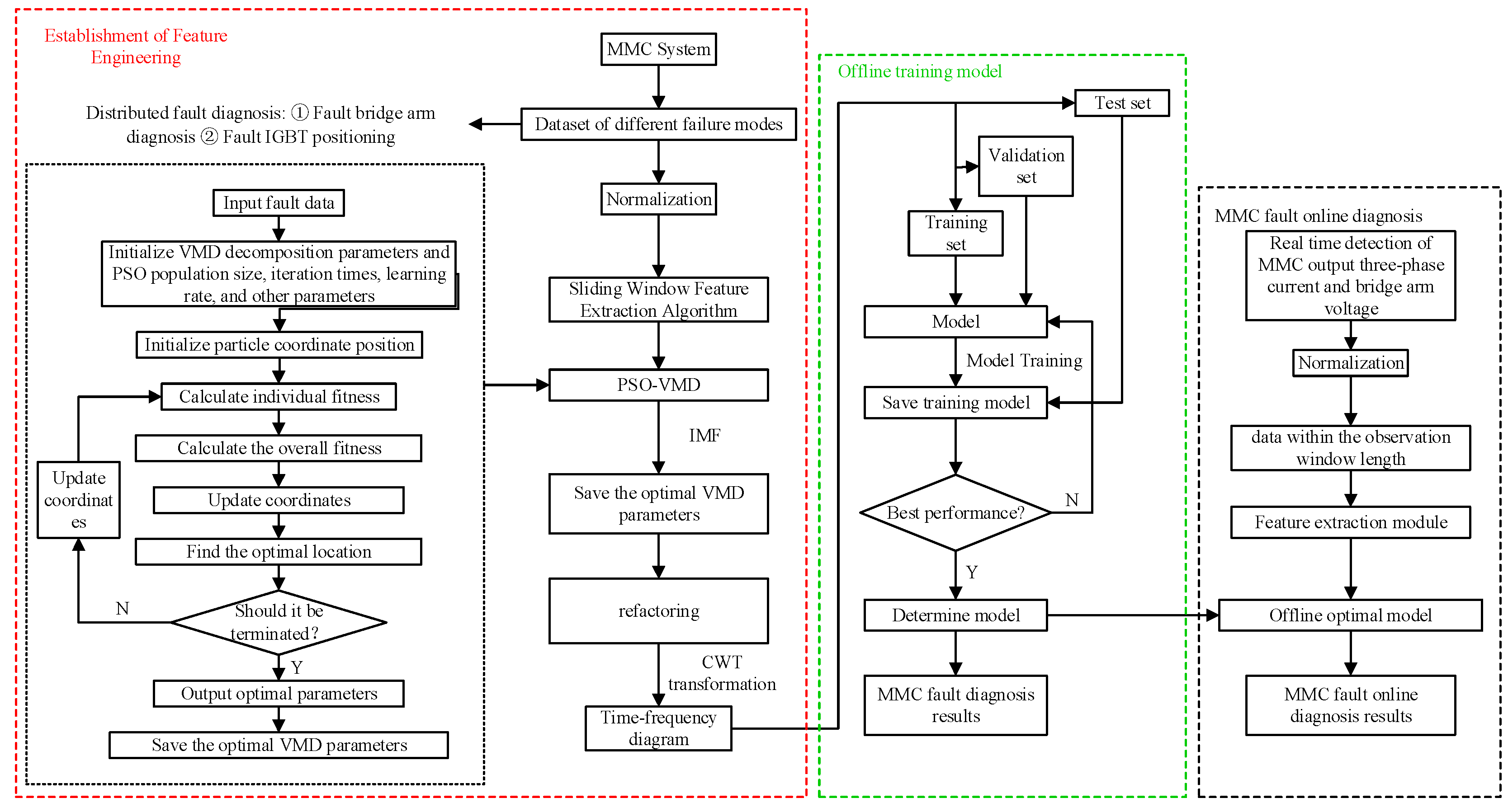
(4) Input the test set into the model saved in step (3) and evaluate the performance of the model. If the evaluation results show that the diagnosis and localization capabilities of the model are not optimal, the model training and validation are returned to step (3) to be repeated until the model performance meets the preset criteria, and a model with optimal performance is finally trained. The model can be subsequently put into the actual MMC work for online fault diagnosis. Figure 8 shows the overall process of MMC fault diagnosis.
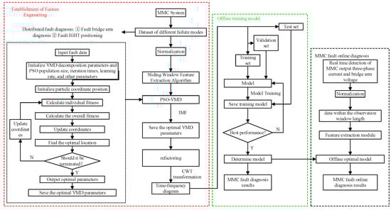
Figure 8.
MMC fault diagnosis overall flowchart.
The design of the whole model takes into account the complexity and diversity of fault diagnosis and effectively improves the accuracy and robustness of the diagnosis through multi-level feature extraction and expression. In addition, the parameter settings of the model need to be optimized according to the actual experimental data to ensure the accuracy and reliability of fault diagnosis.
4. Simulation and Analysis
In order to verify the effectiveness of the MMC submodule open-circuit fault diagnosis method FFT-CNN-BIGRU-Attention based on a modal time–frequency diagram, a three-phase MMC system designed the MATLAB/Simulink platform, (the version number of MATLAB is 2023b) and some of the design parameters of the MMC system and their values are shown in Table 1 and the number of sample labels and fault categories is shown in Table 2.

Table 1.
MMC system partial parameters.
Table 2.
Sample labeling and number of fault categories.
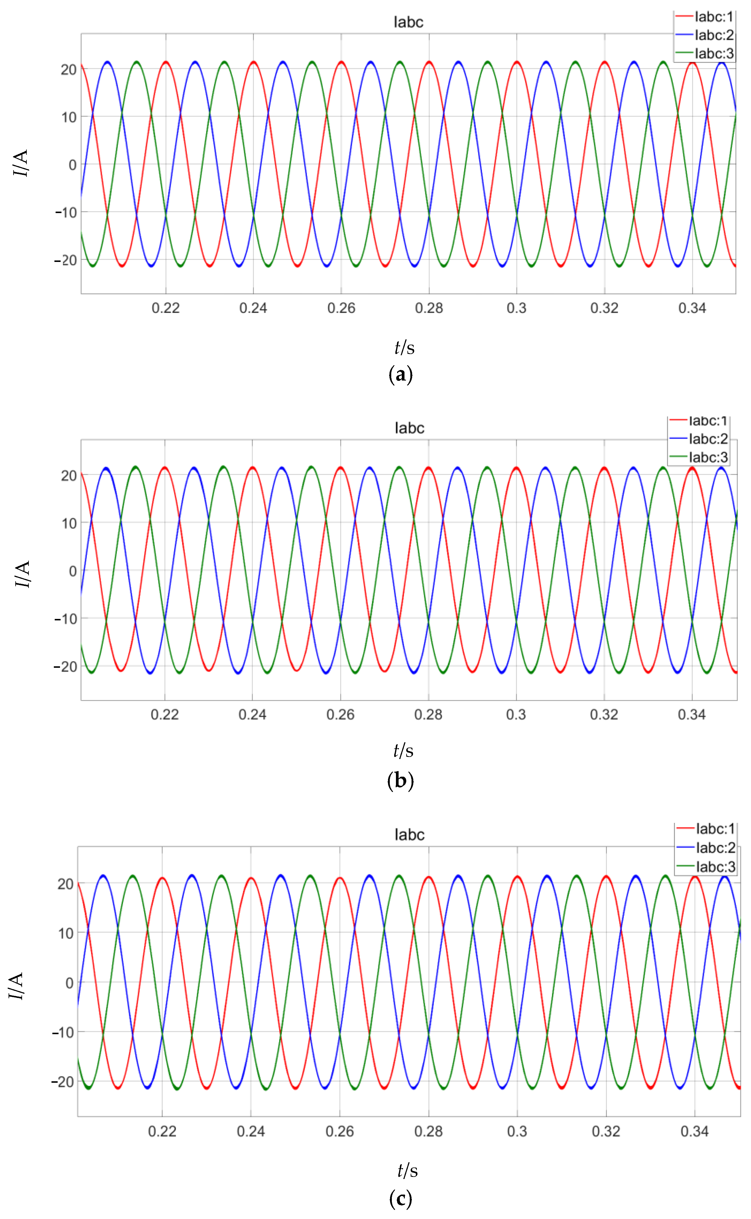
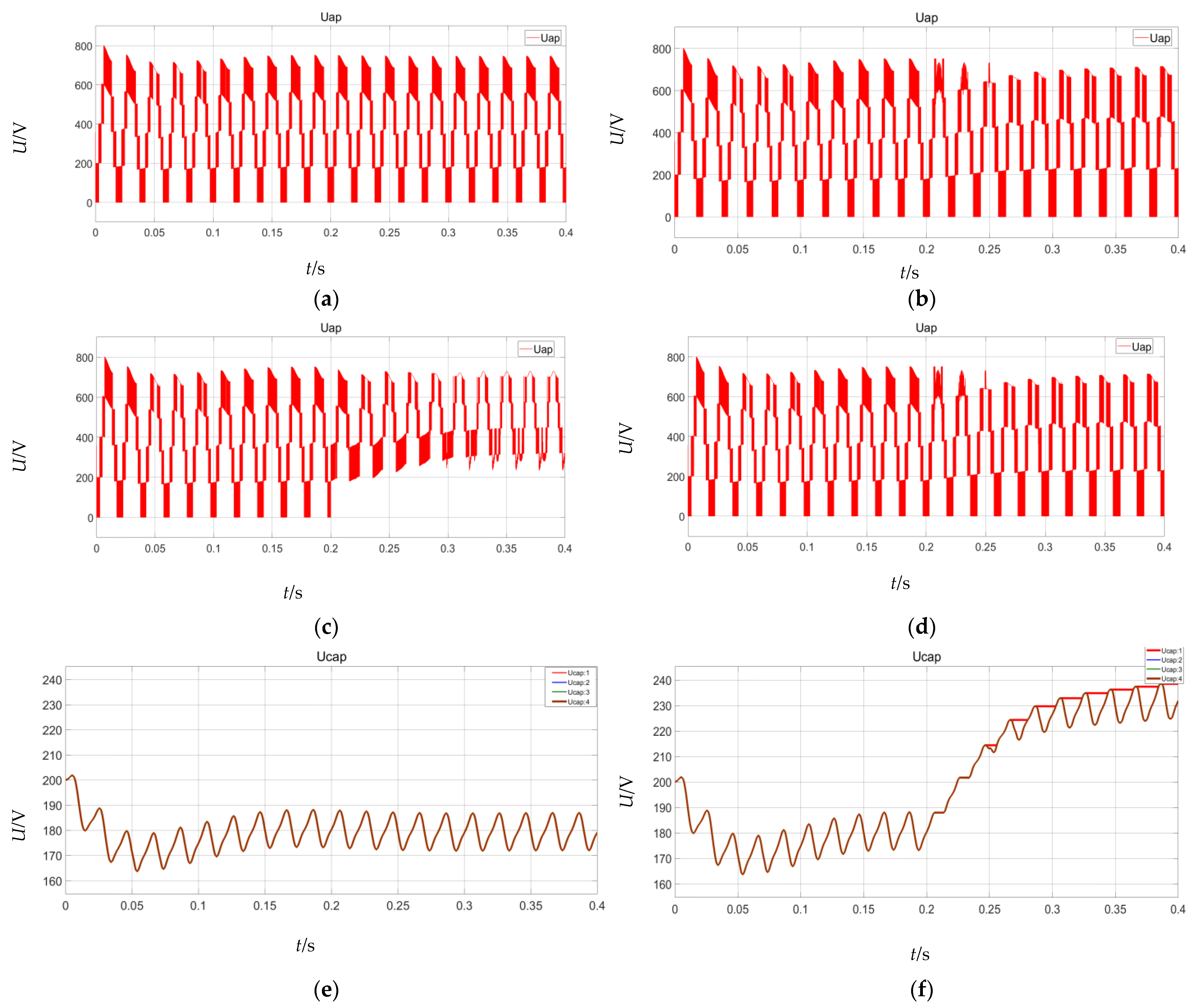
In order to solve the diagnosis problem, it is chosen to simulate the occurrence of open-circuit faults in different IGBT positions at 0.2 s during the operation of the MMC system for 0.4 s. According to the data in Table 3, seven sets of different bridge arm faults can be collected from different phase current data, in which the three-phase output current waveforms under some faults are shown in Figure 9. If the diagnostic results show that the open-circuit fault occurs in a certain phase bridge arm, then it is only necessary to carry out an in-depth study of the bridge arm for that single phase. Taking the open-circuit fault on phase A as an example, according to the data in Table 3, the voltage data of the bridge arm on phase A under nine fault categories can be collected, and the voltage waveforms of the bridge arm on phase A under certain faults are shown in Figure 10.
Table 3.
Performance analysis of different diagnostic methods.
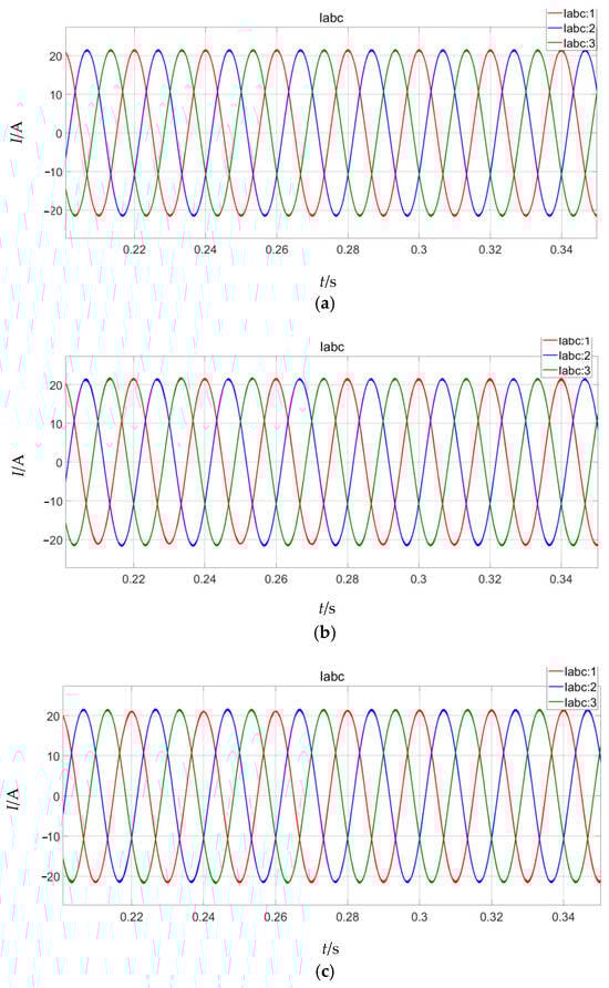
Figure 9.
MMC output phase currents under partial fault categories (a) Normal statement; (b) A_up fault; (c) A_down fault.
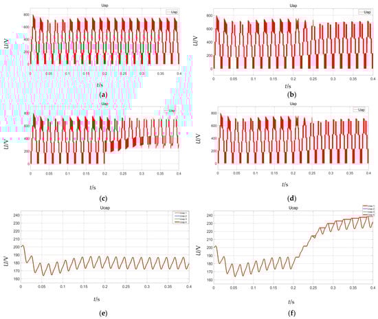
Figure 10.
MMC bridge arm voltages for some fault categories: (a) normal statement of phase voltage; (b) SM1_T1 fault; (c) SM1_T2 fault; (d) SM2_T1 fault; (e) normal statement of capacitor voltage; (f) SM1_T1 fault submodule capacitor voltage.
Figure 9 demonstrates that the difference between the upper and lower bridge arm current waveforms of the same phase in the time domain is small, and it is difficult to mine effective fault information. Figure 10 demonstrates the simulated waveform of the SM1T1 tube in the inverter state when an open-circuit fault occurs at 0.2 s. The figure shows that the capacitive voltage of the faulty submodule continues to rise due to its inability to discharge, while the voltage of the normally operating submodule shows a decreasing trend. This voltage difference causes the faulty bridge arm to exhibit significant voltage fluctuations, compared to the non-faulty bridge arm, which has smaller voltage variation. Moreover, the capacitive voltage equalization control causes the voltages of all submodules in the faulty phase to be perturbed, but the voltage variation characteristics of the submodules of each non-faulty bridge arm are basically the same.
In [14], the authors proposed a sliding window feature-extraction algorithm for processing offline data and dynamically updating fault data so as to expand the sample size. With a total sample size of 200,000, the sliding window length of 2000 sample points and the sliding step length of 250 sample points are designed after comprehensive consideration, so the faulty phase current signal can be divided into 973 samples sequentially. It can be seen from Figure 10 that the IGBTs in different positions in the same sub-module, after an open-circuit fault occurs in the bridge arm voltage, will show obvious distortion, but it is difficult to distinguish the bridge arm voltage change through a time–domain observation after an open-circuit fault occurs in IGBTs in the same position in different sub-modules, so it is necessary to process it with the help of a fine feature extraction method. Similarly, the sliding window length is designed to be 2000 sample points, the sliding step length is 250 sample points, and the faulty bridge arm voltage signal can be divided into 973 samples sequentially.
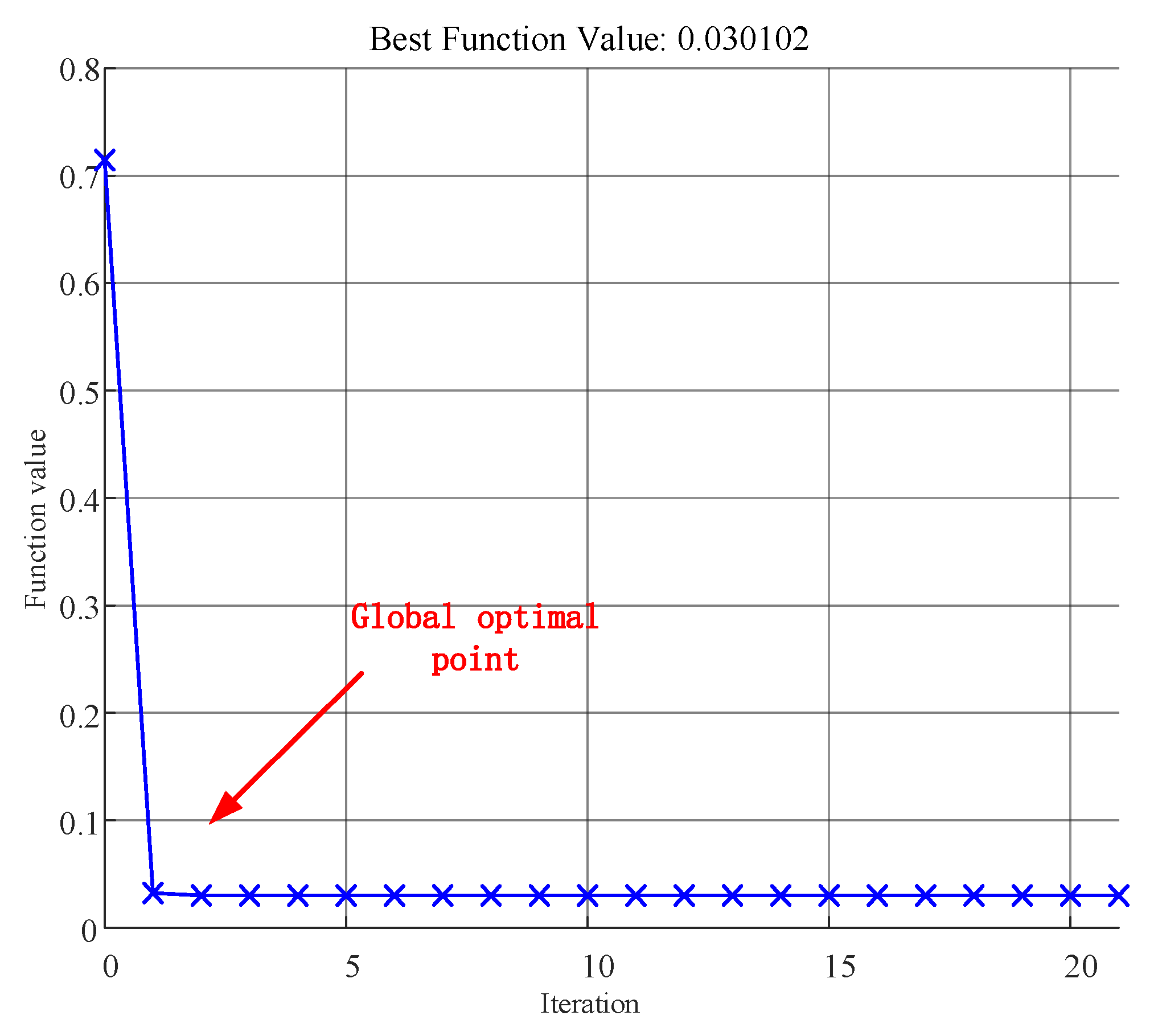
For the phase current samples under different fault categories and bridge arm voltage samples, the PSO-VMD method is used. The bridge on the phase A fault and an open-circuit fault occurring in SM1_T1 are used as examples for the analysis. The results show that the algorithm can reach the global optimum point at the early stage of iteration when locating the faulty IGBTs in the sub-module, and the iteration speed is fast and the performance is excellent, and the convergence is successfully realized. The optimal parameters in the right side of Figure 11 are substituted into the VMD algorithm adaptively occurring in the arm to decompose the MMC fault signal. The decomposition results of the PSO-VMD algorithm under some fault categories are shown in Figure 12.
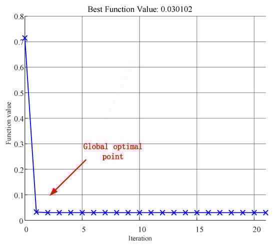
Figure 11.
Optimisation of VMD using Particle Swarm Algorithm algorithm.
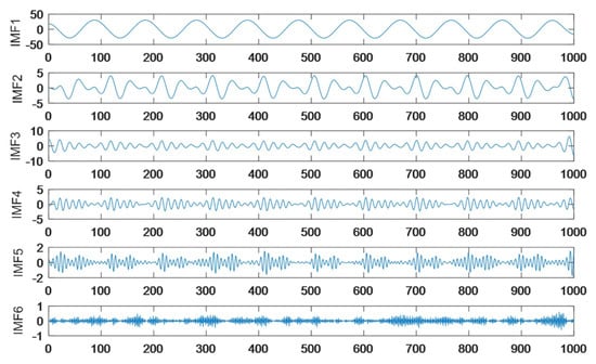
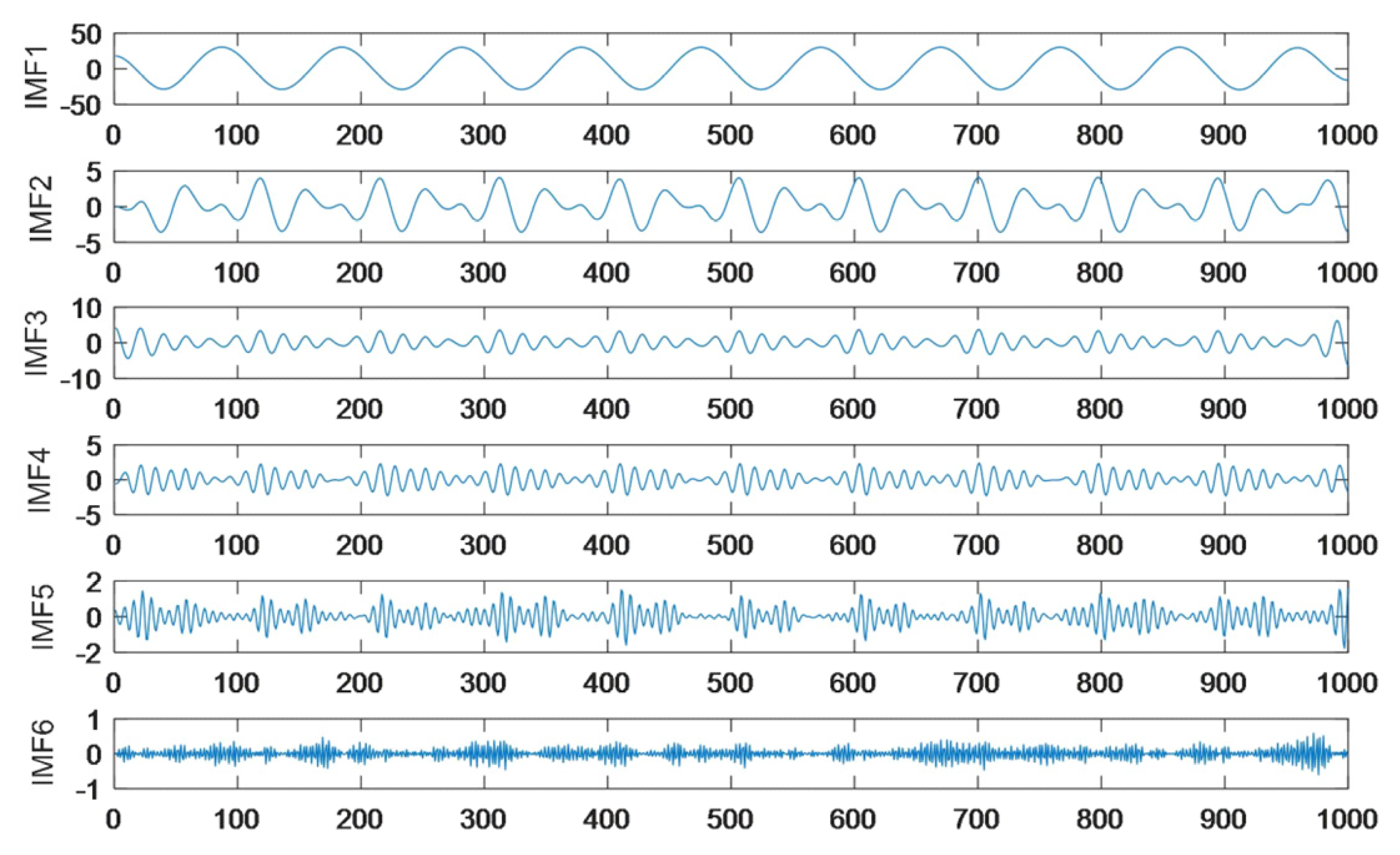
Figure 12.
VMD decomposition diagram for fault signals.
The reconstructed signal is used as the input to the continuous wavelet transform (CWT), where the length of the scale sequence is set to 128, and the wavelet basis function is chosen to be the complex Morlet wavelet, so as to generate the modal time–frequency map of the fault signal. In order to reduce the consumption of computational resources, the resolution of the modal time–frequency diagram is designed to be 150 × 150. The results of the modal time-frequency diagram are shown in Figure 13.
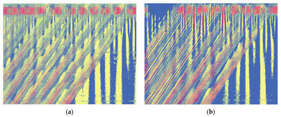
Figure 13.
State modal time–frequency diagram: (a) normal; (b) SM1_T1 in fault.
The dataset 1 and dataset 2 are randomly divided into training and testing sets at a ratio of 7:3, respectively. During the training process of the deep learning model, the dataset is randomly shuffled and the cross-entropy loss function is used to measure the difference between the predicted and actual values. The Adam optimization algorithm is used to dynamically adjust the learning rate based on the historical gradient. The total number of iterations is set to be 150 rounds, and the initial learning rate is 0.001. In order to promote better convergence of the model, the designed learning rate is reduced every round by iterations of 10%, and the number of samples for each iteration is set (batch size) to be 32 to achieve a balance in computational efficiency.
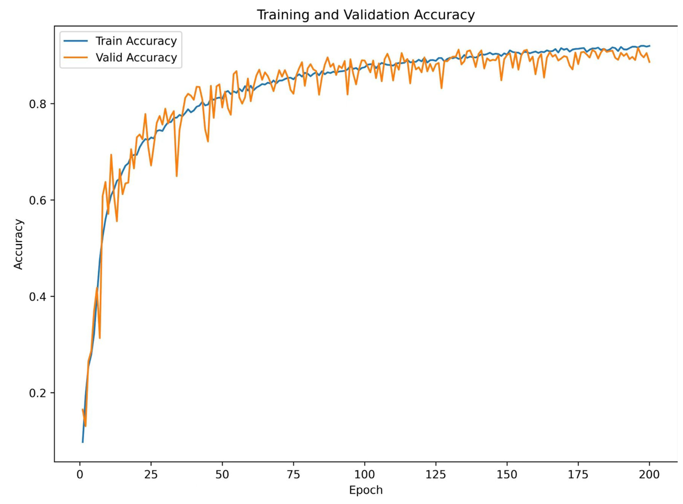
During the training of the model on different datasets, the training accuracy increases rapidly and the loss function value decreases rapidly, indicating that the model can adapt to the training set quickly and effectively learn from the fault features, as shown in Figure 14. At about 35 rounds of iterations, the dataset training accuracy and loss function values both stabilize, and the model begins to converge gradually. After completing 1 dataset and 150 rounds of iterations, the model reaches its optimal performance. For dataset 1, the training accuracy is about 98.63% and the loss rate is about 0.001. At this point, the model not only achieves the convergence state, but also shows great generalization based on different datasets. Given that the model performance reaches optimization at the 150th iteration, the model will be used in subsequent fault diagnosis and localization to achieve the fast identification and processing of IGBT open-circuit faults.
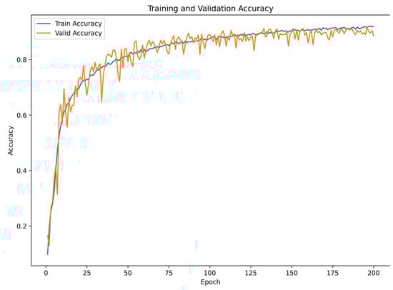
Figure 14.
Accuracy during training.
Considering the length of the diagnosis time, the time of training the model does not affect the performance of the fault diagnosis system, the key is the length of time spent in the online fault diagnosis process. In this paper, different test sets are inputted into the already trained target model, and the average diagnosis time is about 1.48 s as shown in Figure 15.
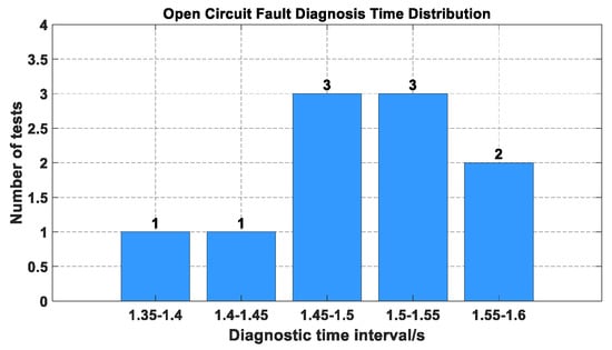
Figure 15.
Average diagnostic time.
Input the test set into the target network and confuse the matrix classification results.
According to Figure 16, the accuracy of the final 810 test samples reached 98.12%. Sample modal time–frequency diagrams under different fault categories can be accurately diagnosed and classified using the diagnostic model, with high recognition accuracy, strong generalization performance, and effective diagnostic occurrence. It can be seen that most of these error cases are evenly distributed and have little impact on the overall diagnostic results. The results indicate that the proposed fault diagnosis method can effectively identify the single open-circuit fault problem of IGBT modules.
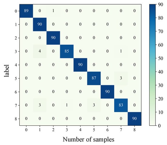
Figure 16.
Confusion matrix of diagnostic results during testing.
In order to assess the diagnostic efficiency of the method more accurately, sub-module open-circuit faults at different locations are set up separately, and 10 groups of sub-module open-circuit fault experimental tests are carried out. The histogram of the fault diagnosis time is shown in Figure 16, and the diagnosis time of the five groups of tests is less than 1.5 s, with an average time of 1.5 s. The submodule can be removed before the open-circuit fault causes substantial harm.
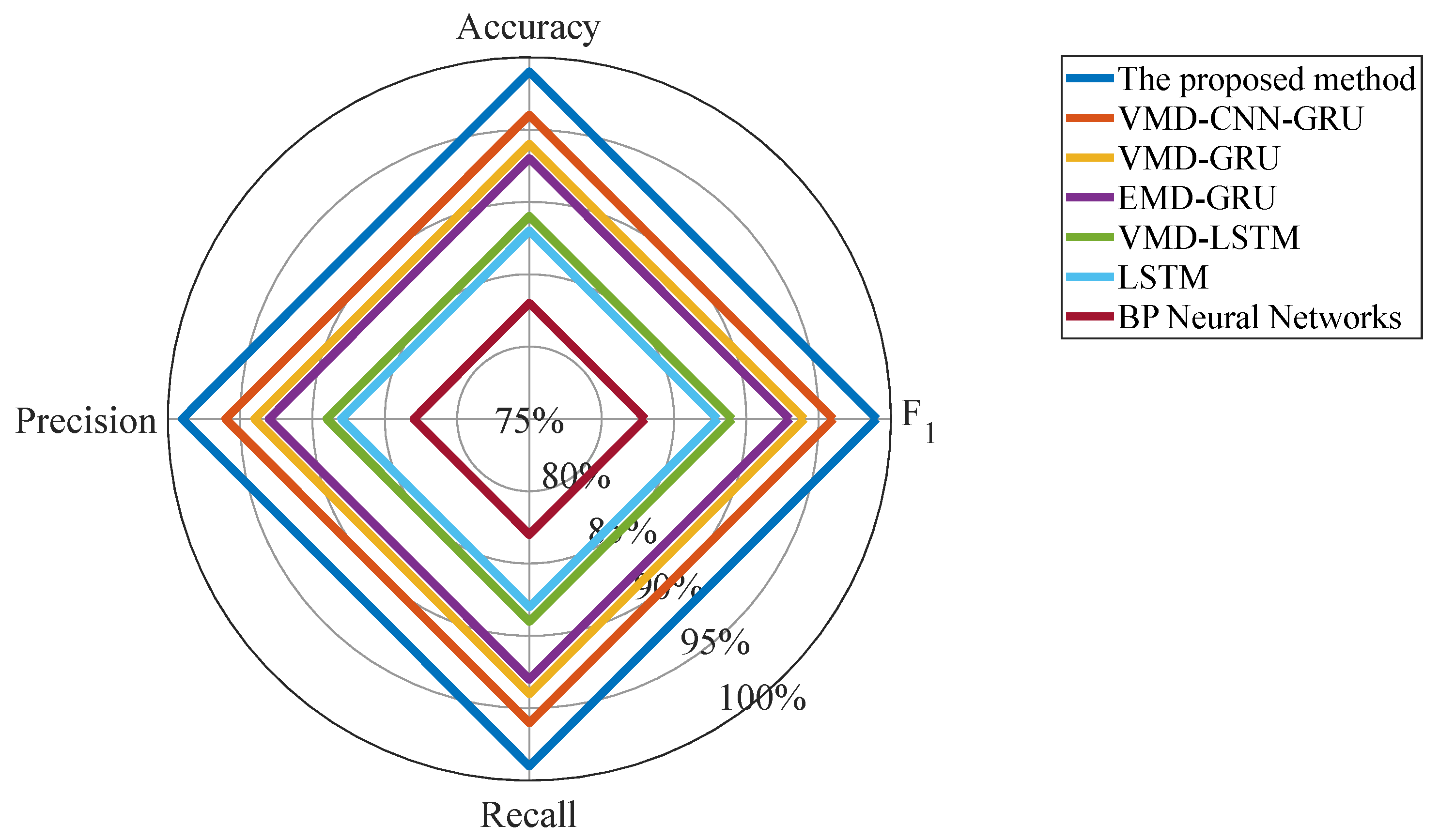
In order to further validate the superiority of the methodology of this paper and to evaluate the fault feature extraction and recognition capability of the model, the performance of the methodology proposed in the literature [14,15,16] was tested against other feature extraction algorithms and classification networks of the fault diagnosis methodology used in this paper, using the same data and based on the training and test sets.
In comparison to the VMD-CNN-GRU model, the BiGRU model possesses a bidirectional structure, enabling it to capture both the forward and backward information of the sequence. This bidirectional structure facilitates a more comprehensive understanding of the sequence’s context, thereby enhancing data comprehension. Compared to the VMD-LSTM and Resnet-BiGRU models, it reveals that the former exhibits superior performance in the domain of long-term dependency modeling. This distinction can be attributed to the gating mechanism inherent to the Resnet-BiGRU model, which facilitates more effective control over the flow of information The maximum number of iterations of the BP neural network is MaxEpoachs = 100, the learning rate is lr = 0.01, and the number of neurons in the hidden layer is determined to be 2n + 1 based on the input dimension n. In the VMD-GRU comparison, the original three-phase current signals are subjected to the Variational Modal Decomposition (VMD) according to the literature [15], and the energy-value features of the modal components of each phase of the current signals are extracted and normalized to form a 1 × 15 feature vector × 15 feature vectors, which are inputted into the BP neural network for training and diagnosis, verifying that the lack of manual feature extraction has a large impact on the fault diagnosis accuracy, and the signal decomposition algorithm in the iterative decomposition affects the fault diagnosis time of the system. Compared with the literature [16], for the single use of the LSTM method in the comparison experiment, the use of cross-entropy as a loss function, and the maximum number of iterations MaxEpoachs = 100, the learning rate is set to 0.01, the batch size is set to 128, due to the three-phase current data length being too large, resulting in slower diagnostic time, and at the same time, suitable feature extraction algorithms can improve the fault diagnosis accuracy. As shown in Figure 17, dataset 1 is used as the input for each model, and the same metrics are selected from the same LSTM to quantitatively analyze the fault diagnosis performance of different models. Each of the seven methods was tested 20 times, and the results are shown in Table 3.
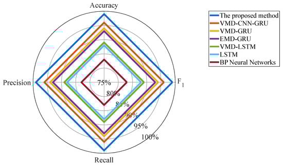
Figure 17.
Evaluation indicators under different models.
The BiGRU model exhibits reduced computational complexity in comparison with the VMD-LSTM model. This reduction is attributed to the BiGRU model’s comparatively simple internal structure, which contains a limited number of parameters. This characteristic leads to enhanced efficiency during the training and testing processes. Under the condition of ensuring the consistency of the diagnostic model, the feature extraction method of constructing a modal time–frequency diagram, adopted in this paper, is better than other schemes in different evaluation indexes, and the accuracy rate is improved by 17.28% and 13.85% compared with BP and LSTM. The optimization of the VMD decomposition of fault signals to generate modal time–frequency diagrams using the particle swarm algorithm successfully makes up for the shortcomings of other algorithms in transforming the lack of feature extraction ability, and modal time–frequency diagrams can more clearly reflect the time–frequency domain characteristics of fault signals, retaining the rich and sensitive information; compared to VMD-LSTM, the VMD-CNN-GRU algorithm diagnostic models designed in this paper are the highest in all evaluation indexes. Compared with the VMD-LSTM model, the proposed model combines the advantages of RNN and CNN, while extracting local features, and the BiGRU model is able to capture global contextual information, and this combination allows for stronger feature extraction when dealing with complex sequential data; this improves the efficiency of the overall diagnosis through a relatively simple internal structure.
5. Results
In this paper, through a comprehensive analysis and three-phase current variation characteristics, a deep learning model combining the optimization of a bridge arm voltage MMC system in a normal state and single bridge arm sub-module open-circuit faults is proposed, and PSO-VMD with FFT-CNN-BiGRU-Attention is applied to the diagnosis and localization of sub-module open-circuit faults. The effectiveness and superiority of the method are verified through a comparative analysis, and the following conclusions are MMC drawn.
Aiming at the problem of fault diagnosis of the MMC sub-module, by using the PSO-VMD algorithm to reasonably select the fault parameters, this both avoids the sudden change in magnitude, reducing the computation amount, and accurately retains the feature information.
Aiming at the problem of the low diagnostic accuracy due to single or missing feature extraction in fault diagnosis, a fault diagnosis method based on feature extraction is proposed by combining the three-phase current and bridge arm voltage. The method enhances the recognition ability of multi-scale feature data, applies the PSO algorithm to optimize the VMD decomposition parameters and obtain the modal time–frequency diagram after decomposition, and introduces the Attention Mechanism in the traditional GRU model to efficiently extract the data features, which provides better fault recognition support for the model FFT-CNN-BIGRU-Attention. The results show that the proposed scheme is a promising algorithm for MMC open-circuit fault diagnosis in terms of the classification accuracy and diagnosis efficiency.
In practical engineering applications, the MMC system structure is highly complex and contains numerous components. In terms of the fault diagnosis accuracy, there is still room for improvement, which is an important subject in our future research. Therefore, the effectiveness of the diagnosis and localization methods in real systems requires further research and MMC validation. Its generalization ability in real industrial environments needs to be further verified.
Author Contributions
Conceptualization, Z.Z.; methodology, Z.Z.; software, Z.Z.; validation, Z.Z.; formal analysis, Z.Z., N.W., S.L., B.Z., and L.G.; investigation, Z.Z.; resources, Z.Z.; data curation, Z.Z.; writing—original draft preparation, Z.Z., S.L., N.W., B.Z., and L.G.; writing—review and editing, Z.Z.; visualization, N.W., B.Z., and L.G.; supervision, N.W., B.Z., and L.G.; project administration, N.W., B.Z., and L.G.; funding acquisition, Z.Z. All authors have read and agreed to the published version of the manuscript.
Funding
This research received no external funding.
Institutional Review Board Statement
Not applicable.
Informed Consent Statement
Not applicable.
Data Availability Statement
Data are contained within the article.
Conflicts of Interest
Bo Zhou was employed by the Huadian New Energy Group Co., Ltd. Lei Guo was employed by the GuangXi LongYuan Renewables Co., Ltd. The authors declare no conflicts of interest.
References
- Liu, X.; Liu, H.; Qiao, H.; Zhou, S.; Qin, L. An Improved Fault Localization Method for Direct Current Filters in HVDC Systems: Development and Application of the DRNCNN Model. Machines 2024, 12, 185. [Google Scholar] [CrossRef]
- Shen, Y.; Wang, T.; Amirat, Y.; Chen, G. IGBT Open-Circuit Fault Diagnosis for MMC Submodules Based on Weighted-Amplitude Permutation Entropy and DS Evidence Fusion Theory. Machines 2021, 9, 317. [Google Scholar] [CrossRef]
- Wang, Q.; Yu, Y.; Ahmed, H.O.; Darwish, M.; Nandi, A.K. Fault detection and classification in MMC-HVDC systems using learning methods. Sensors 2020, 20, 4438. [Google Scholar] [CrossRef]
- Keijo, J.; Stefanie, H.; Daniel, J. Staffan Norrga and Hans-Peter Nee, Comparative evaluation of voltage source converters with silicon carbide semiconductor devices for high-voltage direct current transmission. IEEE Trans. Power Electron. 2021, 36, 8887–8906. [Google Scholar]
- Xu, Y.; Li, S.; Feng, K.; Sun, B.; Yang, X.; Kou, L.; Zhao, Z.; Huang, G.Q. Multiperspective temporal pooling convolutional neural networks for fault diagnosis of mechanical transmission systems. IEEE Trans. Instrum. Meas. 2025, 74, 3517512. [Google Scholar] [CrossRef]
- Chen, X.; Liu, J.; Deng, Z.; Song, S.; Ouyang, S. IGBT Open-Circuit Fault Diagnosis for Modular Multilevel Converter With Reduced-Number of Voltage Sensor Measuring Technique. In Proceedings of the 2019 IEEE 10th International Symposium on Power Electronics for Distributed Generation Systems (PEDG), Xi’an, China, 3–6 June 2019; pp. 47–50. [Google Scholar]
- Pablo, L.; Ricardo, A.; Jose, R. Fault detection on multi-cell converter based on output voltage frequency analysis. IEEE Trans. Ind. Electron. 2009, 56, 2275–2283. [Google Scholar]
- Xu, K.; Xie, S.; Yan, Y.; Zhang, Z.; Zhang, B.; Qian, Q. A fast fault diagnosis method for submodule failures in modular multilevel converters. In Proceedings of the 2017 IEEE Energy Conversion Congress and Exposition (ECCE), Cincinnati, OH, USA, 1–5 October 2017; pp. 1125–1130. [Google Scholar]
- Abdallah, M.M.; Hamad, M.S.; Helal, A.A. Fault detection and isolation of MMC under submodule open circuit fault. In Proceedings of the 2017 Nineteenth International Middle East Power Systems Conference (MEPCON), Cairo, Egypt, 19–21 December 2017; pp. 1195–1200. [Google Scholar]
- Yang, S.; Bryant, A.; Mawby, P.; Xiang, D.; Ran, L.; Tavner, P. An industry-based survey of reliability in power electronic converters. IEEE Trans. Ind. Appl. 2011, 47, 1441–1451. [Google Scholar] [CrossRef]
- Deng, F.; Jin, M.; Liu, C. Switch open-circuit fault localization strategy for MMCs using sliding-time window based features extraction algorithm. IEEE Trans. Ind. Electron. 2021, 68, 10193–10206. [Google Scholar] [CrossRef]
- Gu, J.; Yang, J.; Zhao, C. Fault diagnosis method for wind turbine inverter based on VMD wavelet packet energy entropy. Mech. Res. Appl. 2023, 36, 163167. [Google Scholar] [CrossRef]
- Wang, H.; Liu, Z.; Peng, D.; Cheng, Z. Attention-guided joint learning CNN with noise robustness for bearing fault diagnosis and vibration signal denoising. ISA Trans. 2022, 128, 470–484. [Google Scholar] [CrossRef] [PubMed]
- Zhao, Z.; Jiao, Z. A fault diagnosis method for rotating machinery based on CNN with mixed information. IEEE Trans. Ind. Informat. 2022, 19, 9091–9101. [Google Scholar] [CrossRef]
- Wang, X.; Zhang, D.; Li, M. Fault location method for a hybrid DC transmission system based on wavelet energy spectrum and SSA-GRU. Power Syst. Prot. Control 2023, 51, 14–24. [Google Scholar]
- Yang, Y.; Dong, Z.; Yao, F. Fault diagnosis of double bridge parallel excitation power unit based on 1D-CNN-LSTM hybrid neural network model. Power Syst. Technol. 2021, 45, 2025–2032. [Google Scholar]


Disclaimer/Publisher’s Note: The statements, opinions and data contained in all publications are solely those of the individual author(s) and contributor(s) and not of MDPI and/or the editor(s). MDPI and/or the editor(s) disclaim responsibility for any injury to people or property resulting from any ideas, methods, instructions or products referred to in the content. |
© 2025 by the authors. Licensee MDPI, Basel, Switzerland. This article is an open access article distributed under the terms and conditions of the Creative Commons Attribution (CC BY) license (https://creativecommons.org/licenses/by/4.0/).