Simultaneous Confidence Intervals for Odds Ratios in Bilateral Correlated Data Under Equal Correlation Coefficient Model

Abstract

Bilateral data arising from paired organs or limbs within the same subject frequently occur in clinical trials and biomedical research. Neglecting the intraclass correlation inherent in such data can lead to inaccurate variance estimation and invalid statistical inference. Donner’s equal correlation coefficient model addresses this issue by assuming a single, common intraclass correlation coefficient across all individuals to characterize the dependence between paired observations from the same subject. Although prior research under this model has developed asymptotic testing procedures and confidence interval approaches for two-group comparisons of proportions, simultaneous confidence intervals for the odds ratio have not been thoroughly investigated. This article derives nine asymptotic simultaneous confidence intervals for the odds ratio and evaluates their performance through extensive Monte Carlo simulations, focusing on the empirical coverage probability and mean interval width. A real-world example is presented to illustrate the practical application of the proposed methods.

1. Introduction

In clinical trials and biomedical research, bilateral data frequently arise from paired organs or limbs within the same subject, such as eyes, fingers, legs, or arms. For bilateral diseases, measurements from each side are often treated as independent observational units. Nevertheless, paired observations within the same subject must account for intraclass correlation; failure to account for this correlation can lead to incorrect variance estimation and invalid statistical inference [1,2]. Consequently, statistical methods that appropriately address intraclass correlation are essential for valid inference.

Over the past several decades, the challenge of intraclass correlation has led to the development of various methodological approaches. Model-based approaches, such as the generalized linear mixed model and generalized estimating equations (GEEs), offer valid inferential procedures. Liang and Zeger [3] introduced the concept of a working correlation matrix, together with a sandwich variance estimator, to fit the GEE model for analyzing non-Gaussian data, particularly in longitudinal studies. GEE produces consistent estimates of marginal effects even when the working correlation structure is misspecified, as long as the mean model is correctly specified.

Rosner [4] introduced the ‘constant R model’, which assumes that paired observations from the same participant are dependent. This dependence is characterized by a constant parameter R, defined as the conditional probability that one side is affected given that the other side already is.

However, Dallal [5] questioned the suitability of Rosner’s constant R model, arguing that it performs inadequately when a characteristic is almost certain to occur bilaterally across groups with widely varying prevalence rates. As an alternative, he proposed a model based on compound multinomial sampling, in which the conditional probability of occurrence at one site, given occurrence at the other, stays fixed within each group. It does not scale with the overall prevalence parameter.

Donner [6] subsequently proposed an adjusted chi-square test in which the standard Pearson chi-square statistic is divided by a variance inflation factor derived from an estimated intraclass correlation coefficient. This method assumes a single, constant intraclass correlation coefficient ($\rho$) for all individuals in the sample, thereby accounting for the dependence between paired observations from the same subject. In this model, Ma and Liu [7] introduced three asymptotic testing procedures to evaluate the equality of proportions across multiple groups. To address the limitations of asymptotic methods in small sample contexts, Liu et al. [8] developed five exact methods.

As confidence intervals provide information on both the magnitude and precision of estimates, making them more informative than point estimates alone in statistical analysis. Several scholars have contributed to the development and application of confidence intervals in this field. For example, Newcombe [9] proposed 10 methods based on asymptotic theory and exact approaches for differences in proportions, thereby establishing a foundational framework that has influenced subsequent research. Tang et al. [10] later developed three confidence intervals using the method of variance estimates recovery. Similarly, Pei et al. [11] proposed five asymptotic confidence interval methods for estimating the difference in proportions between two treatment groups based on the $\rho$ model. Building on this work, Tang et al. introduced a series of confidence interval methods based on Newcombe, Rosner, and Pei’s model [12,13,14]. Additionally, Tang et al. [15] extended the literature by constructing eight confidence intervals specifically designed for incomplete paired bilateral data structures.

Additionally, in oncology clinical trials using master protocols, such as umbrella trials that evaluate multiple treatments concurrently within a single disease indication, the United States Food and Drug Administration recommends incorporating a common control arm to enhance trial efficiency. These designs enable the simultaneous assessment of several experimental treatments against a shared control group [16]. Within this context, simultaneous confidence intervals (SCIs) have been widely studied. Peng [17] and Yang [18] developed asymptotic SCIs of odds ratio (OR) and proportion differences based on the R model. Yang [19] developed asymptotic SCIs of proportion differences based on the $\rho$ model.

The OR is a fundamental statistical measure that quantifies the strength of association between an exposure and a disease outcome, serving a role analogous to that of relative risk [20]. In addition, the OR is the primary measure of effect in case–control studies where the incidence of disease cannot be directly estimated, and thus relative risk and attributable risk cannot be determined [21,22]. Therefore, this article extends the discussion on methods of constructing SCIs for the OR within the framework of the $\rho$ model.

The rest of this article is organized as follows. The Methods Section introduces three approaches for constructing SCIs—the Wald-type, profile likelihood, and asymptotic score methods—together with their corresponding multiplicity adjustment approaches. The Simulation Studies section presents performance evaluations of these methods in terms of empirical coverage probability (ECP) and mean interval width (MIW). The Real Case Example section illustrates the practical application of the proposed methods through a real data analysis. The final section summarizes the key findings and discusses their implications.

2. Methods

2.1. Data Structure

Suppose that the goal is to evaluate the effectiveness of multiple treatments. Let $m_{li}$ denote the number of patients in the group $i(i=1,2,\dots ,g$) who have $l(l=0,1,2)$ responses, and let $m_i={\sum }_{l=0}^2{m}_{li}$ be the fixed total number of patients in the group i. Define $S_l={\sum }_{i=1}^g{m}_{li}$ as the total number of patients across all groups with a response l, and let N denote the total number of patients in the research study. Patients are randomly assigned to the g treatment groups. The data structure is presented in Table 1.

Table 1. Data structure in a bilateral design.

Number of Responses (l)	Group (l)				Total
	1	2	⋯	$\mathit{g}$
0	$m_{01}$	$m_{02}$	⋯	$m_{0g}$	$S_0$
1	$m_{11}$	$m_{12}$	⋯	$m_{1g}$	$S_1$
2	$m_{21}$	$m_{22}$	⋯	$m_{2g}$	$S_2$
Total	$m_1$	$m_2$	⋯	$m_g$	N

Define $Z_{ijk}$ as the dummy response variable for the kth body part (e.g., eye) $(k=1,2)$ of the jth individual in the ith treatment group, where $i=1,2,\dots ,g$. This variable $\left(Z_{ijk}\right)$ takes the value of one if the event occurs and zero otherwise.

Under the constant correlation coefficient model introduced by Donner [6], the disease rates are assumed to be identical within each group. Let $\rho$ denote the common correlation coefficient, and let $\mathrm{Pr}\left(Z_{ijk}=1\right)$ denote the probability of a positive response for the kth eye of a patient in the ith group:

$$\begin{array}{c}\mathrm{Pr}\left(Z_{ijk}=1\right)={\pi }_i;i=1,\dots ,g;j=1,\dots ,m_i;0\le {\pi }_i\le 1\hfill \\ \mathrm{Corr}\left(Z_{ijk},Z_{ij(3-k)}\right)=\rho ,0\le \rho \le 1\hfill \end{array}$$

Within each group, the observation frequencies ${\mathit{m}}_i=(m_{0i},m_{1i},m_{2i})$ follow a multinomial distribution:

$$\begin{array}{c}\hfill f\left(m_{0i},m_{1i},m_{2i}\right)={\displaystyle \frac{m_i!}{m_{0i}!m_{1i}!m_{2i}!}}{p}_{0i}^{m_{0i}}{p}_{1i}^{m_{1i}}{p}_{2i}^{m_{2i}},\end{array}$$

where the cell probabilities $p_{li}$ are determined by ${\pi }_i$ and $\rho$:

$$\left\{\begin{array}{cc}& p_{0i}=(1-{\pi }_i)(\rho {\pi }_i-{\pi }_i+1),\hfill \\ & p_{1i}=2{\pi }_i(1-\rho )(1-{\pi }_i),\hfill \\ & p_{2i}={\pi }_i^2+\rho {\pi }_i(1-{\pi }_i),\hfill \end{array}\right.$$

(1)

in which ($l=$ 0, 1, 2, $i=$ 1, 2,$\cdots ,g$), which together sum to one for any fixed i.

In this paper, we wish to construct the SCIs for $O{R}_i$, considering the first group as a control group and the OR between any treatment groups and the control group defined as $O{R}_i=o_i/o_1={\displaystyle \frac{{\pi }_i/(1-{\pi }_i)}{{\pi }_1/(1-{\pi }_1)}}(i=2,\dots ,g)$. Here, $o_i$ represents the odds of the ith group.

The corresponding log-likelihood function can be written as follows:

$$\begin{array}{cc}\hfill l_1({\pi }_1,\cdots ,{\pi }_g;\rho )=& {\displaystyle \sum _{i=1}^g}[m_{2i}\log ({{\pi }_i}^2-{\pi }_i\rho \left({\pi }_i-1\right))+m_{1i}\log (2{\pi }_i\left({\pi }_i-1\right)\left(\rho -1\right))\hfill \\ \hfill +& m_{0i}\log (-\left({\pi }_i-1\right)\left({\pi }_i\rho -{\pi }_i+1\right)]+\log C,\hfill \end{array}$$

(2)

where $C={\prod }_{i=1}^g({\displaystyle \frac{m_i!}{m_{0i}!m_{1i}!m_{2i}!}})$ is a constant.

By substituting ${\pi }_i={({\displaystyle \frac{1}{O{R}_i·o_i}}+1)}^{-1}={({\displaystyle \frac{1-{\pi }_1}{O{R}_i·{\pi }_1}}+1)}^{-1}(i=2,\cdots ,g)$ into $l_1$, the log-likelihood function can be rewritten as follows:

$$\begin{array}{c}\hfill \begin{array}{cc}\hfill l_2(O{R}_i,\overrightarrow{\mathsf{\pi }},\rho )& ={\displaystyle \sum _{j=1,j\ne i}^g}[m_{2j}\log \left({{\pi }_j}^2-{\pi }_j\rho \left({\pi }_j-1\right)\right)\hfill \\ & + m_{1j}\log \left(2{\pi }_j\left({\pi }_j-1\right)\left(\rho -1\right)\right)\hfill \\ & + m_{0j}\log \left(-\left({\pi }_j-1\right)\left({\pi }_j\rho -{\pi }_j+1\right)\right)]\hfill \\ & + m_{2i}\log \left({\left({\displaystyle \frac{1-{\pi }_1}{O{R}_i·{\pi }_1}}+1\right)}^{-2}+{\left({\displaystyle \frac{1-{\pi }_1}{O{R}_i·{\pi }_1}}+1\right)}^{-1}\rho {\left({\displaystyle \frac{O{R}_i{\pi }_1}{1-{\pi }_1}}+1\right)}^{-1}\right)\hfill \\ & + m_{1i}\log \left(2\left({\displaystyle \frac{1-{\pi }_1}{O{R}_i·{\pi }_1}}+1\right){\left({\displaystyle \frac{O{R}_i{\pi }_1}{1-{\pi }_1}}+1\right)}^{-1}\left(1-\rho \right)\right)\hfill \\ & + m_{0i}\log \left({\left({\displaystyle \frac{O{R}_i{\pi }_1}{1-{\pi }_1}}+1\right)}^{-1}[{\left({\displaystyle \frac{1-{\pi }_1}{O{R}_i·{\pi }_1}}+1\right)}^{-1}\rho +{\left({\displaystyle \frac{O{R}_i{\pi }_1}{1-{\pi }_1}}+1\right)}^{-1}]\right),\hfill \end{array}\end{array}$$

(3)

where $\overrightarrow{\mathsf{\pi }}=({\pi }_1,\cdots ,{\pi }_{i-1},{\pi }_{i+1},\cdots ,{\pi }_g)$, $O{R}_i(i=2,\cdots ,g)$ denotes the parameter of interest and ${\pi }_j(j\ne i)$ and $\rho$ are treated as nuisance parameters.

2.2. Multiplicity Adjustment

Performing multiple statistical tests concurrently leads to substantial inflation of the Type I error rate relative to the nominal significance level of each individual test. The application of suitable multiplicity adjustments is therefore necessary to ensure the validity and reliability of the overall statistical conclusions drawn from the analysis. As described by the data structure mentioned above, there are g groups in total: one control group and $g-1$ treatment groups. The primary objective is to assess treatment effectiveness by comparing the OR between each treatment and the common control groups. A widely used approach for controlling multiplicity is the Bonferroni correction. The Bonferroni correction controls the family-wise error rate (FWER) without requiring assumptions of the dependence structure among the individual comparisons, although it may be conservative. This property makes the procedure applicable to the present setting without requiring additional assumptions. For $g-1$ simultaneous comparisons at an overall significance level $\alpha$, the Bonferroni-adjusted critical value is $c=z_{1-\alpha /\left(2\right(g-1\left)\right)}$, where z denotes the standard normal distribution.

Another method considered in this study is the Šidák correction [23], which is closely related to the Bonferroni correction but is generally less conservative. Under independence, the Šidák procedure provides exact simultaneous coverage. For $g-1$ simultaneous comparisons at an overall significance level $\alpha$, the corresponding critical value $c=z_{1-\left[{(1-\alpha )}^{1/(g-1)}\right]/2}$, where z denotes the standard normal distribution.

The third method adopted in this study draws upon the framework of the Dunnett test. Dunnett [24] developed a multiple comparison procedure for comparing several treatments with a common control which directly corresponds to the many-to-one comparison structure considered here. The Dunnett procedure accounts for correlation among comparisons through their joint distribution. Following this framework, Piegorsch [25] proposed a general procedure for constructing SCIs for proportion differences. Here, we apply this method to derive the corresponding SCIs formulas for the OR. Let $a_i$ denote the log odds ($a_i=\log o_i$ for the ith group), and reformulate the problem from log-OR to log odds differences, namely $a_2-a_1$,…, $a_g-a_1$. The SCI of the odds ratio $O{R}_i=o_i/o_1$ is then obtained by exponentiating the corresponding confidence limits on the log-OR scale. The critical value $c={\left|z\right|}_{g-1;\mathbb{R}}^{\alpha }$ equals $1-\alpha /2$ quantile of the $g-1$ variate normal distribution with a mean equal to zero and correlation matrix $\mathbb{R}$$=\left\{{\rho }_{ij}\right\}$, ${\rho }_{ij}={\omega }_i{\omega }_j$, and

$${\omega }_i={\left[1+{\displaystyle \frac{m_1}{m_i}}{\displaystyle \frac{\widehat{{\pi }_1}\left(1-\widehat{{\pi }_1}\right)}{\widehat{{\pi }_i}\left(1-\widehat{{\pi }_i}\right)}}\right]}^{-1/2}.$$

Overall, the Bonferroni, Šidák, and Dunnett procedures provide complementary approaches to multiplicity adjustment for the many-to-one comparison setting considered in this study. Their different treatments of the dependence among multiple comparisons provide a useful basis for constructing and comparing SCIs for multiple treatment-versus-control comparisons.

2.3. Wald-Type Confidence Interval

Ma and Liu [7] derived the maximum likelihood estimator (MLE) of $({\pi }_1,\dots ,{\pi }_g,\rho )$ using a third-order polynomial and the Fisher scoring method. Following a similar approach, we can derive the MLE of ($\log \left(o_1\right),\dots ,\log \left(o_g\right),\log (\rho /(1-\rho ))$). By applying the logarithmic property that log(${\mathit{OR}}_i$) = $\log \left(o_i\right)-\log \left(o_1\right)$, together with the invariant property of the MLE, the MLE of the OR can be obtained through a linear transformation. Let $\mathsf{\beta }=\left(\log \right(o_1$),…, $\log \left(o_g\right)$, $\log \left(\rho /(1-\rho )\right))$, and the unconstrained MLE of $\mathsf{\beta }$ be denoted by $\widehat{\mathsf{\beta }}=\left(\log \right({\widehat{o}}_1$),…, $\log \left({\widehat{o}}_g\right)$, $\log \left(\widehat{\rho }/(1-\widehat{\rho })\right))$. Thus, the MLE of $\log \left(OR\right)$ is log$(\widehat{{\mathit{OR}}_i})={\mathit{K}}_i{\widehat{\mathsf{\beta }}}^T$, where ${\mathit{K}}_i$ denotes the ith row of the matrix $\mathit{K}$:

$${\mathit{K}}_{(\mathit{g}-\mathbf{1})\times (\mathit{g}+\mathbf{1})}=\left[\begin{array}{ccccccc}-1& 1& 0& \cdots & 0& 0& 0\\ -1& 0& 1& \cdots & 0& 0& 0\\ ⋮& ⋮& ⋮& \ddots & ⋮& ⋮& ⋮\\ -1& 0& 0& \cdots & 1& 0& 0\\ -1& 0& 0& \cdots & 0& 1& 0\end{array}\right].$$

The standard error of log($o_i$), for $i=1,2,\dots ,g,$ can be estimated from $\widehat{{\pi }_i}$ by applying the delta method. Let $\mathsf{\gamma }=({\pi }_1,\cdots ,{\pi }_g,\rho )$ denote the parameter, with its corresponding MLE of $\mathsf{\gamma }$ being $\widehat{\mathsf{\gamma }}$. Under the asymptotic normality of the MLE, it can be shown that

$$\sqrt{n}(\widehat{\mathsf{\gamma }}-\mathsf{\gamma })\stackrel{\mathrm{d}}{\to }N(0,{\mathit{I}}^{-1}),$$

where $\mathit{I}$ denotes the Fisher information matrix of $\mathsf{\gamma }$.

Applying the delta method yields

$$\sqrt{n}(\widehat{\mathsf{\beta }}-\mathsf{\beta })\stackrel{\mathrm{d}}{\to }N(0,g{\mathit{I}}^{-1}{g}^T),$$

where $g=$ Diag(${\displaystyle \frac{1}{\widehat{{\pi }_1}}}+{\displaystyle \frac{1}{1-\widehat{{\pi }_1}}},\cdots ,{\displaystyle \frac{1}{\widehat{{\pi }_g}}}+{\displaystyle \frac{1}{1-\widehat{{\pi }_g}}},{\displaystyle \frac{1}{\widehat{\rho }}}+{\displaystyle \frac{1}{1-\widehat{\rho }}}$). Therefore, the $100(1-\alpha )$% SCI for $\log \left(O{R}_i\right)$ is given by

$${\mathit{K}}_{\mathit{i}}{\widehat{\mathsf{\beta }}}^{\mathit{T}}\pm c\sqrt{{\mathit{K}}_{\mathit{i}}\left[g{\widehat{\mathit{I}}}^{-1}{g}^T\right]{\mathit{K}}_{\mathit{i}}^{\mathit{T}}},$$

where c is the critical value and $\widehat{\mathit{I}}$ denotes the Fisher information matrix estimator. Through a simple transformation, the $100(1-\alpha )$% SCI for $O{R}_i$ is given by

$${\exp }^{({\mathit{K}}_{\mathit{i}}{\widehat{\mathsf{\beta }}}^{\mathit{T}}\pm c\sqrt{{\mathit{K}}_{\mathit{i}}\left[g{\widehat{\mathit{I}}}^{-1}{g}^T\right]{\mathit{K}}_{\mathit{i}}^{\mathit{T}}})}.$$

When the Bonferroni method is applied to control the FWER at a level $\alpha$, the corresponding critical value is given by

$$c=z_{1-\alpha /\left(2(g-1)\right)},$$

where z denotes the standard normal distribution.

When the Šidák method is used instead, the critical value is

$$c=z_{1-{\alpha }^{\prime }/2},{\alpha }^{\prime }=1-{(1-\alpha )}^{\left(1/(g-1)\right)},$$

where z denotes the standard normal distribution.

In addition, when the Dunnett method is used, the critical value is

$$c={\left|z\right|}_{g-1;\mathbb{R}}^{\alpha },$$

where $\left|z\right|$ denotes the $1-\alpha /2$ quantile of the $g-1$ variate normal distribution with the correlation structure, as specified in the previous section.

2.4. Profile Likelihood Confidence Interval

The asymptotic profile likelihood SCI for each OR ($O{R}_i,i=2,\dots ,g$) can be constructed from the chi-square distribution by inverting the likelihood ratio test of a hypothesis $H_0:O{R}_i=O{R}_0$ versus $H_a:O{R}_i\ne O{R}_0,i=2,\dots ,g$. Without loss of generality, we first set $i=2$, and we start by calculating the CI for the OR between the second group and the control group.

Let (${\widetilde{OR}}_2,\widetilde{{\pi }_1},\widetilde{{\pi }_3},\dots ,\widetilde{{\pi }_g},\tilde{\rho }$) denote the constrained MLEs of ($O{R}_2,{\pi }_1,{\pi }_3,\dots ,{\pi }_g,\rho$) obtained under the null hypothesis, and let (${\widehat{OR}}_2,{\widehat{\pi }}_1,{\widehat{\pi }}_3,\dots ,{\widehat{\pi }}_g,\widehat{\rho }$) denote the corresponding unconstrained MLEs obtained under the alternative hypothesis. The likelihood ratio test statistic is then given by

$$T_L=2\left[l_2({\widehat{OR}}_2,{\widehat{\pi }}_1,{\widehat{\pi }}_3,\dots ,{\widehat{\pi }}_g,\widehat{\rho })-l_2({\widetilde{OR}}_2,{\tilde{\pi }}_1,{\tilde{\pi }}_3,\dots ,{\tilde{\pi }}_g,\tilde{\rho })\right].$$

Setting the partial differentiation of $l_2$ with respect to ${\pi }_i$ and $\rho$ equal to zero yields the MLEs of the corresponding parameters:

$$\begin{array}{cc}& {\left.{\displaystyle \frac{\partial l_2}{\partial {\pi }_i}}\right|}_{O{R}_2=O{R}_0}=0,(i=1,3,\dots ,g),\hfill \\ & {\left.{\displaystyle \frac{\partial l_2}{\partial \rho }}\right|}_{O{R}_2=O{R}_0}=0.\hfill \end{array}$$

These estimators ($\widetilde{{\pi }_1},\widetilde{{\pi }_3},\dots ,\widetilde{{\pi }_g},\tilde{\rho }$) can be obtained, subject to the constraint that $O{R}_2=O{R}_0$. As no closed-form solution exists, the constrained MLEs are obtained numerically via the Fisher scoring algorithm:

$$\left[\begin{array}{c}{\pi }_1^{(t+1)}\\ {\pi }_3^{(t+1)}\\ ⋮\\ {\pi }_g^{(t+1)}\\ {\rho }^{(t+1)}\end{array}\right]=\left[\begin{array}{c}{\pi }_1^{\left(t\right)}\\ {\pi }_3^{\left(t\right)}\\ ⋮\\ {\pi }_g^{\left(t\right)}\\ {\rho }^{\left(t\right)}\end{array}\right]+{\left.{\mathit{I}}^{-1}\left({\pi }_1^{\left(t\right)},{\pi }_3^{\left(t\right)},\dots ,{\pi }_g^{\left(t\right)},{\rho }^{\left(t\right)}\right)\left[\begin{array}{c}{\displaystyle \frac{\partial l_2}{\partial {\pi }_1}}\\ {\displaystyle \frac{\partial l_2}{\partial {\pi }_3}}\\ ⋮\\ {\displaystyle \frac{\partial l_2}{\partial {\pi }_g}}\\ {\displaystyle \frac{\partial l_2}{\partial \rho }}\end{array}\right]\right|}_{\left({\pi }_i={\pi }_i^{\left(t\right)},\rho ={\rho }^{\left(t\right)}\right)},$$

where $\mathit{I}\left({\pi }_1^{\left(t\right)},{\pi }_3^{\left(t\right)},\dots ,{\pi }_g^{\left(t\right)},{\rho }^{\left(t\right)}\right)$ denotes the $g\times g$ Fisher information matrix estimated under the condition of (${\pi }_1,{\pi }_3,\dots ,{\pi }_g,\rho$) = (${\pi }_1^{\left(t\right)},{\pi }_3^{\left(t\right)},\dots ,{\pi }_g^{\left(t\right)},{\rho }^{\left(t\right)}$). Under standard regularity conditions, the corresponding test statistic asymptotically follows a chi-square distribution with one degree of freedom. Therefore, the $100(1-\alpha )\%$ profile likelihood SCI for the $O{R}_i$ is derived based on the chi-square distribution and satisfies

$$2(l_2({\widehat{OR}}_2,{\widehat{\pi }}_1,{\widehat{\pi }}_3,\dots ,{\widehat{\pi }}_g,\widehat{\rho })-l_2(O{R}_0,{\tilde{\pi }}_1,{\tilde{\pi }}_3,\dots ,{\tilde{\pi }}_g,\tilde{\rho }))\le {\chi }_{1,1-\alpha /(g-1)}^2,$$

where ${\chi }_{1,1-\alpha /(g-1)}^2$ denotes the $1-\alpha /(g-1)$ quantile of the chi-square distribution with one degree of freedom under Bonferroni multiplicity adjustment. Since ${\chi }_{1,1-\alpha /(g-1)}^2=(z_{1-\alpha /\left(2\right(g-1\left)\right)}{)}^2$, where $(z_{1-\alpha /\left(2\right(g-1\left)\right)}{)}^2$ is the corresponding quantile of the standard normal distribution, similarly, the Šidák method can be implemented by substituting the critical value ${\chi }_{1-\alpha /(g-1)}^2$ with ${\chi }_{1-{\alpha }^{\prime }}$, where ${\alpha }^{\prime }=1-{(1-\alpha )}^{(1/(g-1))}$. Furthermore, Dunnett’s multiplicity adjustment can be applied by substituting the critical value $z_{1-\alpha /\left(2\right(g-1\left)\right)}$ with ${\left|z\right|}_{g-1;\mathbb{R}}^{\alpha }$, which corresponds to the upper $\alpha$ quantile of the multivariate normal distribution with a correlation structure $\mathbb{R}$.

Unlike the Wald-type CI, the lower and upper bounds of the profile likelihood CI are computed separately. The two corresponding roots are obtained via Algorithm 1. Here, we use the upper bound as an example.

Algorithm 1 Bisection method for the upper bound of $O{R}_2$.

Require: Data, significance level $\alpha$, number of groups g, convergence threshold $\epsilon$ (e.g., ${10}^{-5}$)

1: Compute the unconstrained MLEs $({\widehat{OR}}_2,{\widehat{\pi }}_1,{\widehat{\pi }}_3,\dots ,{\widehat{\pi }}_g,\widehat{\rho })$.   2: Initialize $(O{R}_2^{\left(0\right)},{\pi }_1^{\left(0\right)},{\pi }_3^{\left(0\right)},\dots ,{\pi }_g^{\left(0\right)},{\rho }^{\left(0\right)})\leftarrow ({\widehat{OR}}_2,{\widehat{\pi }}_1,{\widehat{\pi }}_3,\dots ,{\widehat{\pi }}_g,\widehat{\rho })$.   3: $flag\leftarrow 1$, $stepsize\leftarrow 0.1$, $t\leftarrow 0$. while $stepsize>\epsilon$      (a) ${\widehat{OR}}_2^{(t+1)}\leftarrow {\widehat{OR}}_2^{\left(t\right)}+flag\times stepsize$.      (b) Compute the constrained MLEs $({\tilde{\pi }}_1^{(t+1)},{\tilde{\pi }}_3^{(t+1)},\dots ,{\tilde{\pi }}_g^{(t+1)},{\tilde{\rho }}^{(t+1)})$ with $O{R}_2={\widehat{OR}}_2^{(t+1)}$.      (c) Compute     T = $2[l_2({\widehat{OR}}_2,{\widehat{\pi }}_1,{\widehat{\pi }}_3,\dots ,{\widehat{\pi }}_g,\widehat{\rho })-l_2({\widehat{OR}}_2^{(t+1)},{\tilde{\pi }}_1^{(t+1)},{\tilde{\pi }}_3^{(t+1)},\dots ,{\tilde{\pi }}_g^{(t+1)},{\tilde{\rho }}^{(t+1)})].$      (d) if $flag\times T<flag\times {\chi }_{1,1-\alpha /(g-1)}^2$             $t\leftarrow t+1$.          ▹ Accept the update and continue searching.             else $flag\leftarrow -flag$, $stepsize\leftarrow 0.1\times stepsize$, $t\leftarrow t+1$.     end while   4: return ${\widehat{OR}}_2^{(t+1)}$.                   ▹ Upper bound of $O{R}_2$.

To obtain the smaller root, which is the lower bound of the CI, repeat steps 1–5, and set the initial value of the direction indicator $flag=-1$.

2.5. Asymptotic Score Confidence Interval

The null hypothesis is

$$H_0:O{R}_i=O{R}_0$$

versus the alternative hypothesis, which is

$$H_a:O{R}_i\ne O{R}_0,i=2,\dots ,g.$$

Under regularity conditions, the asymptotic score test statistic can be derived as follows:

$$T_S^2=\mathit{U}{\mathit{I}}^{-1}{\mathit{U}}^T{|}_{O{R}_i=O{R}_0,\overrightarrow{\mathsf{\pi }}=\widetilde{\overrightarrow{\mathsf{\pi }}},\rho =\tilde{\rho }},$$

where $\mathit{U}$ denotes the score vector, which is obtained from the first derivative of the log-likelihood function with respect to the model parameters, and $\mathit{I}$ represents the Fisher information matrix evaluated under the null hypothesis.

For simplicity, we focus on the case $i=2$, where the score vector is defined by

$$\mathit{U}=\left({\displaystyle \frac{\partial l_2}{\partial O{R}_2}},{\displaystyle \frac{\partial l_2}{\partial {\pi }_1}},{\displaystyle \frac{\partial l_2}{\partial {\pi }_3}},\dots ,{\displaystyle \frac{\partial l_2}{\partial {\pi }_g}},{\displaystyle \frac{\partial l_2}{\partial \rho }}\right),$$

where $l_2$ denotes the log-likelihood function defined previously and the model parameters are $(O{R}_i,\overrightarrow{\mathsf{\pi }},\rho )$, where $\overrightarrow{\mathsf{\pi }}=({\pi }_1,\dots ,{\pi }_{i-1},{\pi }_{i+1},\dots ,{\pi }_g)$. Here, $O{R}_2$ is the parameter of interest, and $\overrightarrow{\mathsf{\pi }},\rho$ are nuisance parameters. The score test statistic can be rewritten as follows:

$$T_S^2={\left.{\left({\displaystyle \frac{\partial l_2}{\partial O{R}_2}}\right)}^2{\mathit{I}}^{-1}(1,1)\right|}_{O{R}_i=O{R}_0},$$

with ${\mathit{I}}^{-1}(1,1)$ denoting the $(1,1)$th element of the inverse Fisher information matrix. See Appendix A for more detail. $T_S^2$ asymptotically follows a chi-square distribution with one degree of freedom. Therefore, $100(1-\alpha )$% SCI for $O{R}_i$ satisfies

$$\{O{R}_0|T_S^2\left(O{R}_0\right)\le {\chi }_{1-\alpha /\left(2\right(g-1\left)\right)}^2\},$$

where the critical value is adjusted to account for multiplicity. Similar to the profile likelihood approach, the confidence limits are obtained numerically using the iterative procedure described in the previous section. At each iteration, the score test statistic is updated with the newly computed Fisher information matrix:

$$\mathit{I}=\mathit{I}\left({\widehat{O{R}_2}}^{\left(t\right)},{\widehat{{\pi }_1}}^{\left(t\right)},{\widehat{{\pi }_3}}^{\left(t\right)},\dots ,{\widehat{{\pi }_g}}^{\left(t\right)},{\widehat{\rho }}^{\left(t\right)}\right).$$

To control the FWER when conducting multiple comparisons, multiplicity adjustment methods such as the Bonferroni correction, Šidák correction, and Dunnett’s procedure are applied as outlined in the previous section.

3. Simulation Studies

We investigate the performance of three proposed statistical methods for constructing SCIs via Monte Carlo simulation studies. Performance was evaluated using two metrics: the ECP and MIW. Both balanced (equal $m_i$) and unbalanced (unequal $m_i$) designs were considered, with all parameter configurations summarized in Table 2.

Table 2. Parameter configuration settings for the simulation study.

Group	$\mathsf{\rho }$	${\mathsf{\pi }}_1,{\mathsf{\pi }}_2,\cdots ,{\mathsf{\pi }}_{\mathit{g}}$	${\mathit{m}}_1,{\mathit{m}}_2,\cdots ,{\mathit{m}}_{\mathit{g}}$
$g=3$	0.3, 0.5, 0.7	a. (0.4, 0.4, 0.4)	I. (50, 50, 50)
		b. (0.3, 0.35, 0.5)	II. (30, 50, 80)
			III. (30, 100, 500)
$g=4$		a. (0.4, 0.4, 0.4, 0.4)	I. (50, 50, 50, 50)
		b. (0.25, 0.3, 0.4, 0.5)	II. (30, 50, 80, 100)
			III. (30, 50, 100, 500)
$g=5$		a. (0.4, 0.4, 0.4, 0.4, 0.4)	I. (50, 50, 50, 50, 50)
		b. (0.25, 0.3, 0.38, 0.45, 0.5)	II. (30, 45, 60, 75, 90)
			III. (30, 50, 100, 200, 500)

In each configuration, 10,000 Monte Carlo samples were generated, and 95% confidence intervals were constructed for each replication. The ECP is defined as the proportion of replications in which the true odds ratio is contained within the constructed SCIs. The MIW is the average width of the SCIs across all replications. Following [26,27], and considering the nominal level of $\alpha =$ 0.05, a method was classified as conservative when its ECP substantially exceeded 0.96, liberal when it fell considerably below 0.94, and recommended when it maintained proximity to 0.95:

$$\begin{array}{c}ECP={\displaystyle \frac{1}{B}}{\sum }_{b=1}^B{\prod }_{i=1}^{g-1}\mathbb{I}(O{R}_i\in (O{R}_{L,i}^{\left(b\right)},O{R}_{U,i}^{\left(b\right)})),\\ MIW={\displaystyle \frac{1}{B(g-1)}}{\sum }_{b=1}^B{\sum }_{i=1}^{g-1}(O{R}_{U,i}^{\left(b\right)}-O{R}_{L,i}^{\left(b\right)}),\end{array}$$

where $\mathbb{I}(·)$ denotes the indicator function, B denotes the total number of replication, and b denotes the bth number of replications $(b=1,\dots ,B$). $O{R}_{L,i}^{\left(b\right)}$ and $O{R}_{U,i}^{\left(b\right)}$ denote the lower and upper bound of $O{R}_i$ between the first group and ith group in the bth replication, respectively.

Table 3, Table 4 and Table 5 present the ECPs and MIWs for the $g=$ 3, 4, and 5 groups, respectively. The ECPs of the Profile–Dunnett method and the Score–Dunnett method remained consistently close to the prespecified nominal level of 0.95 across most simulation scenarios. The Profile–Bonferroni, Profile–Šidák, Score–Bonferroni, and Score–Šidák methods also showed satisfactory performance, particularly in the setting of a group size equal to three and four. In contrast, the Wald-based methods tended to be conservative, with ECPs generally exceeding the nominal level of 0.95 for the majority of the parameter configurations.

Table 3. The empirical coverage probability (ECP) and the mean interval width (MIW) of 95% simultaneous confidence intervals (SCIs) for the odds ratio ($g=3$).

$\mathsf{\rho },\mathsf{\pi },\mathbf{m}$			Wald–Bonferroni		Wald–Dunnett		Wald–Šidák
			ECP	MIW	ECP	MIW	ECP	MIW
0.3	a	I	0.951	1.713	0.949	1.687	0.951	1.708
		II	0.957	1.994	0.955	1.979	0.957	1.988
	b	I	0.954	3.266	0.952	3.223	0.954	3.257
		II	0.962	3.831	0.960	3.806	0.961	3.820
		III	0.968	3.382	0.968	3.374	0.968	3.373
0.5	a	I	0.953	1.887	0.949	1.858	0.952	1.882
		II	0.957	2.217	0.955	2.201	0.956	2.211
	b	I	0.954	3.618	0.952	3.569	0.953	3.609
		II	0.960	4.249	0.958	4.223	0.959	4.237
		III	0.968	3.742	0.967	3.733	0.967	3.732
0.7	a	I	0.954	2.060	0.950	2.028	0.953	2.055
		II	0.960	2.439	0.958	2.420	0.959	2.432
	b	I	0.954	3.970	0.952	3.915	0.954	3.959
		II	0.962	4.672	0.961	4.642	0.962	4.659
		III	0.971	4.103	0.971	4.093	0.971	4.091
$\mathsf{\rho },\mathsf{\pi },\mathbf{m}$			Profile–Bonferroni		Profile–Dunnett		Profile–Šidák
			ECP	MIW	ECP	MIW	ECP	MIW
0.3	a	I	0.949	1.743	0.946	1.717	0.949	1.739
		II	0.953	2.044	0.952	2.029	0.952	2.039
	b	I	0.951	3.320	0.947	3.274	0.950	3.311
		II	0.956	3.977	0.954	3.951	0.955	3.967
		III	0.957	3.546	0.956	3.537	0.956	3.536
0.5	a	I	0.948	1.912	0.944	1.882	0.948	1.907
		II	0.950	2.265	0.949	2.248	0.950	2.258
	b	I	0.948	3.671	0.946	3.621	0.948	3.661
		II	0.952	4.397	0.949	4.366	0.951	4.383
		III	0.954	3.933	0.954	3.924	0.954	3.923
0.7	a	1	0.950	2.078	0.945	2.045	0.949	2.072
		11	0.951	2.487	0.949	2.467	0.951	2.480
	b	I	0.947	4.033	0.944	3.975	0.946	4.021
		II	0.948	4.837	0.947	4.806	0.948	4.826
		III	0.952	4.303	0.953	4.295	0.953	4.293
$\mathsf{\rho },\mathsf{\pi },\mathbf{m}$			Score–Bonferroni		Score–Dunnett		Score–Šidák
			ECP	MIW	ECP	MIW	ECP	MIW
0.3	a	I	0.952	1.698	0.949	1.672	0.951	1.700
		II	0.956	1.966	0.955	1.952	0.956	1.973
	b	I	0.952	3.244	0.950	3.202	0.952	3.236
		II	0.959	3.792	0.958	3.768	0.959	3.783
		III	0.965	3.347	0.964	3.339	0.965	3.339
0.5	a	I	0.951	1.862	0.947	1.834	0.950	1.868
		II	0.955	2.168	0.954	2.152	0.955	2.180
	b	I	0.951	3.575	0.948	3.527	0.951	3.566
		II	0.955	4.172	0.954	4.147	0.955	4.162
		III	0.963	3.679	0.963	3.671	0.963	3.670
0.7	a	I	0.952	2.017	0.948	1.987	0.952	2.028
		II	0.957	2.358	0.955	2.341	0.956	2.381
	b	I	0.948	3.902	0.946	3.849	0.949	3.892
		II	0.954	4.552	0.953	4.523	0.954	4.541
		III	0.967	3.996	0.966	3.987	0.966	3.986

a: π = (0.4, 0.4, 0.4). b: π = (0.3, 0.35, 0.5). I: m = (50, 50, 50). II: m = (30, 50, 80). III: m = (30, 100, 500).

Table 4. The empirical coverage probability (ECP) and the mean interval width (MIW) of 95% SCIs for the odds ratio ($g=4$).

$\mathsf{\rho },\mathsf{\pi },\mathbf{m}$			Wald–Bonferroni		Wald–Dunnett		Wald–Šidák
			ECP	MIW	ECP	MIW	ECP	MIW
0.3	a	I	0.957	1.845	0.952	1.805	0.956	1.840
		II	0.964	2.119	0.962	2.101	0.963	2.113
	b	I	0.959	4.337	0.955	4.262	0.959	4.325
		II	0.972	5.075	0.971	5.039	0.971	5.058
		III	0.971	4.810	0.971	4.788	0.971	4.795
0.5	a	I	0.958	2.038	0.953	1.992	0.957	2.031
		II	0.966	2.348	0.964	2.327	0.965	2.340
	b	I	0.960	4.786	0.956	4.700	0.959	4.771
		II	0.972	5.550	0.971	5.513	0.972	5.533
		III	0.973	5.245	0.972	5.223	0.973	5.230
0.7	a	I	0.961	2.228	0.956	2.177	0.960	2.221
		II	0.967	2.584	0.965	2.560	0.966	2.575
	b	I	0.963	5.221	0.959	5.129	0.963	5.205
		II	0.975	6.003	0.974	5.960	0.975	5.982
		III	0.974	5.722	0.974	5.696	0.974	5.704
$\mathsf{\rho },\mathsf{\pi },\mathbf{m}$			Profile–Bonferroni		Profile–Dunnett		Profile–Šidák
			ECP	MIW	ECP	MIW	ECP	MIW
0.3	a	I	0.955	1.879	0.949	1.838	0.954	1.873
		II	0.951	2.172	0.949	2.152	0.950	2.164
	b	I	0.953	4.433	0.949	4.354	0.952	4.419
		II	0.963	5.327	0.962	5.288	0.963	5.310
		III	0.962	5.099	0.962	5.076	0.962	5.083
0.5	a	I	0.953	2.064	0.948	2.018	0.953	2.057
		II	0.948	2.395	0.946	2.372	0.947	2.387
	b	I	0.953	4.886	0.949	4.797	0.952	4.871
		II	0.959	5.806	0.958	5.765	0.959	5.790
		III	0.961	5.580	0.960	5.554	0.960	5.562
0.7	a	1	0.954	2.241	0.948	2.190	0.953	2.234
		11	0.946	2.635	0.944	2.610	0.945	2.625
	b	I	0.952	5.335	0.947	5.236	0.951	5.320
		II	0.957	6.260	0.956	6.216	0.956	6.242
		III	0.960	5.950	0.959	5.923	0.960	5.933
$\mathsf{\rho },\mathsf{\pi },\mathbf{m}$			Score–Bonferroni		Score–Dunnett		Score–Šidák
			ECP	MIW	ECP	MIW	ECP	MIW
0.3	a	I	0.957	1.834	0.952	1.793	0.956	1.834
		II	0.961	2.092	0.960	2.074	0.961	2.097
	b	I	0.957	4.293	0.952	4.220	0.956	4.280
		II	0.969	4.991	0.968	4.959	0.969	4.977
		III	0.967	4.722	0.965	4.702	0.966	4.708
0.5	a	I	0.957	2.018	0.951	1.973	0.956	2.019
		II	0.963	2.304	0.961	2.284	0.963	2.311
	b	I	0.956	4.712	0.953	4.630	0.955	4.698
		II	0.967	5.413	0.966	5.378	0.967	5.397
		III	0.968	5.138	0.968	5.115	0.968	5.122
0.7	a	I	0.958	2.196	0.954	2.146	0.958	2.199
		II	0.963	2.508	0.961	2.486	0.963	2.522
	b	I	0.957	5.119	0.953	5.032	0.956	5.106
		II	0.968	5.813	0.967	5.781	0.967	5.799
		III	0.968	5.533	0.967	5.508	0.967	5.515

a: π = (0.4, 0.4, 0.4, 0.4). b: π = (0.25, 0.3, 0.4, 0.5). I: m = (50, 50, 50, 50). II: m = (30, 50, 80, 100). III: m = (30, 50, 100, 500).

Table 5. The empirical coverage probability (ECP) and the mean interval width (MIW) of 95% SCIs for the odds ratio ($g=5$).

$\mathsf{\rho },\mathsf{\pi },\mathbf{m}$			Wald–Bonferroni		Wald–Dunnett		Wald–Šidák
			ECP	MIW	ECP	MIW	ECP	MIW
0.3	a	I	0.957	1.945	0.950	1.893	0.956	1.938
		II	0.965	2.289	0.963	2.262	0.964	2.281
	b	I	0.963	4.665	0.958	4.567	0.962	4.650
		II	0.969	5.578	0.967	5.525	0.968	5.558
		III	0.972	5.136	0.972	5.112	0.972	5.119
0.5	a	I	0.961	2.157	0.953	2.098	0.960	2.149
		II	0.968	2.548	0.966	2.517	0.968	2.539
	b	I	0.962	5.180	0.957	5.070	0.961	5.162
		II	0.974	6.088	0.972	6.033	0.973	6.067
		III	0.977	5.561	0.977	5.537	0.977	5.545
0.7	a	I	0.963	2.359	0.958	2.293	0.963	2.351
		II	0.966	2.823	0.964	2.788	0.965	2.813
	b	I	0.965	5.685	0.961	5.566	0.964	5.666
		II	0.973	6.562	0.971	6.503	0.972	6.543
		III	0.980	6.088	0.980	6.061	0.980	6.070
$\mathsf{\rho },\mathsf{\pi },\mathbf{m}$			Profile–Bonferroni		Profile–Dunnett		Profile–Šidák
			ECP	MIW	ECP	MIW	ECP	MIW
0.3	a	I	0.951	1.975	0.944	1.922	0.950	1.969
		II	0.953	2.345	0.951	2.317	0.952	2.337
	b	I	0.954	4.782	0.949	4.677	0.954	4.766
		II	0.958	5.855	0.956	5.799	0.957	5.835
		III	0.966	5.489	0.965	5.461	0.966	5.469
0.5	a	I	0.954	2.179	0.944	2.120	0.953	2.172
		II	0.951	2.600	0.948	2.567	0.950	2.590
	b	I	0.951	5.307	0.946	5.194	0.950	5.288
		II	0.959	6.385	0.958	6.325	0.958	6.365
		III	0.964	5.940	0.963	5.912	0.963	5.921
0.7	a	1	0.952	2.366	0.945	2.300	0.951	2.358
		11	0.940	2.883	0.937	2.844	0.939	2.872
	b	I	0.954	5.811	0.948	5.687	0.952	5.793
		II	0.957	6.805	0.954	6.747	0.956	6.781
		III	0.967	6.393	0.966	6.356	0.966	6.367
$\mathsf{\rho },\mathsf{\pi },\mathbf{m}$			Score–Bonferroni		Score–Dunnett		Score–Šidák
			ECP	MIW	ECP	MIW	ECP	MIW
0.3	a	I	0.955	1.935	0.948	1.884	0.955	1.932
		II	0.963	2.262	0.961	2.236	0.963	2.264
	b	I	0.960	4.612	0.955	4.517	0.960	4.596
		II	0.964	5.474	0.962	5.426	0.964	5.456
		III	0.969	5.035	0.968	5.015	0.968	5.021
0.5	a	I	0.958	2.140	0.950	2.082	0.957	2.137
		II	0.966	2.505	0.964	2.476	0.965	2.507
	b	I	0.958	5.090	0.951	4.987	0.957	5.073
		II	0.969	5.925	0.967	5.876	0.968	5.907
		III	0.971	5.431	0.970	5.410	0.970	5.417
0.7	a	I	0.959	2.328	0.953	2.265	0.959	2.327
		II	0.960	2.752	0.957	2.719	0.960	2.755
	b	I	0.959	5.554	0.954	5.441	0.958	5.537
		II	0.965	6.323	0.963	6.274	0.964	6.305
		III	0.975	5.863	0.974	5.838	0.974	5.846

a: $\mathsf{\pi }=(0.4,0.4,0.4,0.4,0.4).$ b: $\mathsf{\pi }=(0.25,0.3,0.38,0.45,0.5).$ I: $\mathit{m}=(50,50,50,50,50).$ II: $\mathit{m}=(30,45,60,75,90).$ III: $\mathit{m}=(30,50,100,200,500).$

The MIWs showed generally similar patterns across the simulation scenarios. Compared with the profile likelihood method, the score method tended to produce slightly narrower intervals across all scenarios. In general, balanced designs yielded ECPs closer to the nominal level and were accompanied by narrower MIWs.

Overall, among the three multiplicity adjustments considered, the Dunnett adjustment generally provided ECPs closer to the nominal level while maintaining relatively narrow MIWs. Considering both the ECP and MIW, the score method combined with the Dunnett adjustment showed favorable overall performance and may therefore be preferred for practical implementation.

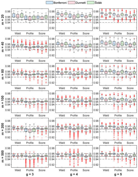
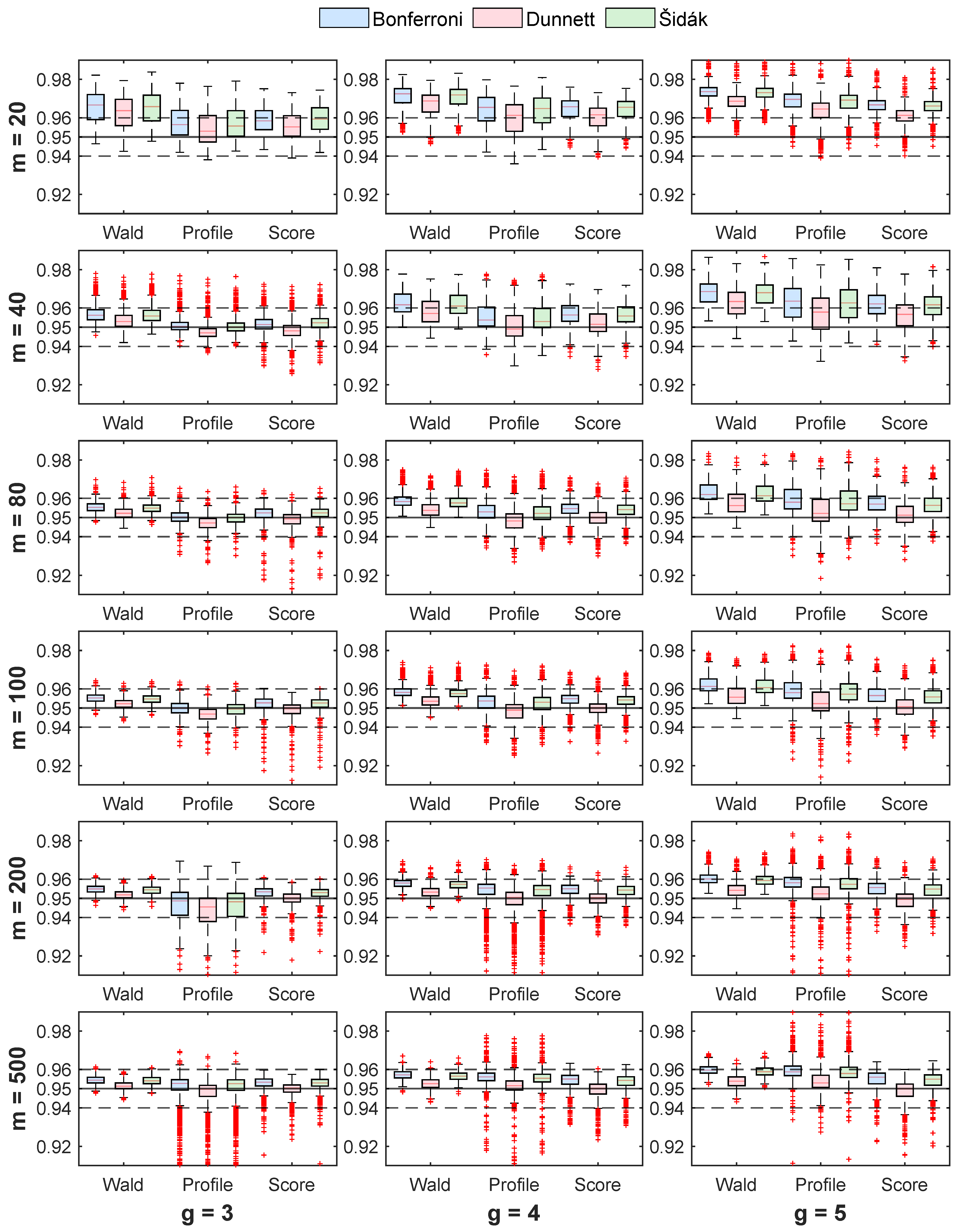
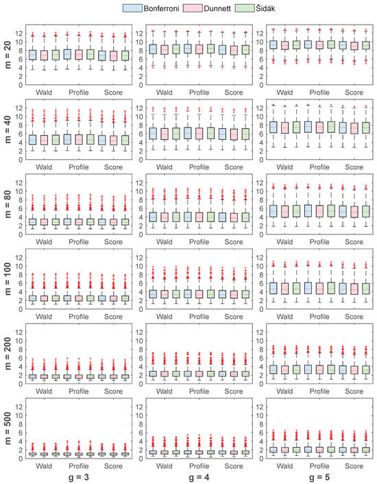
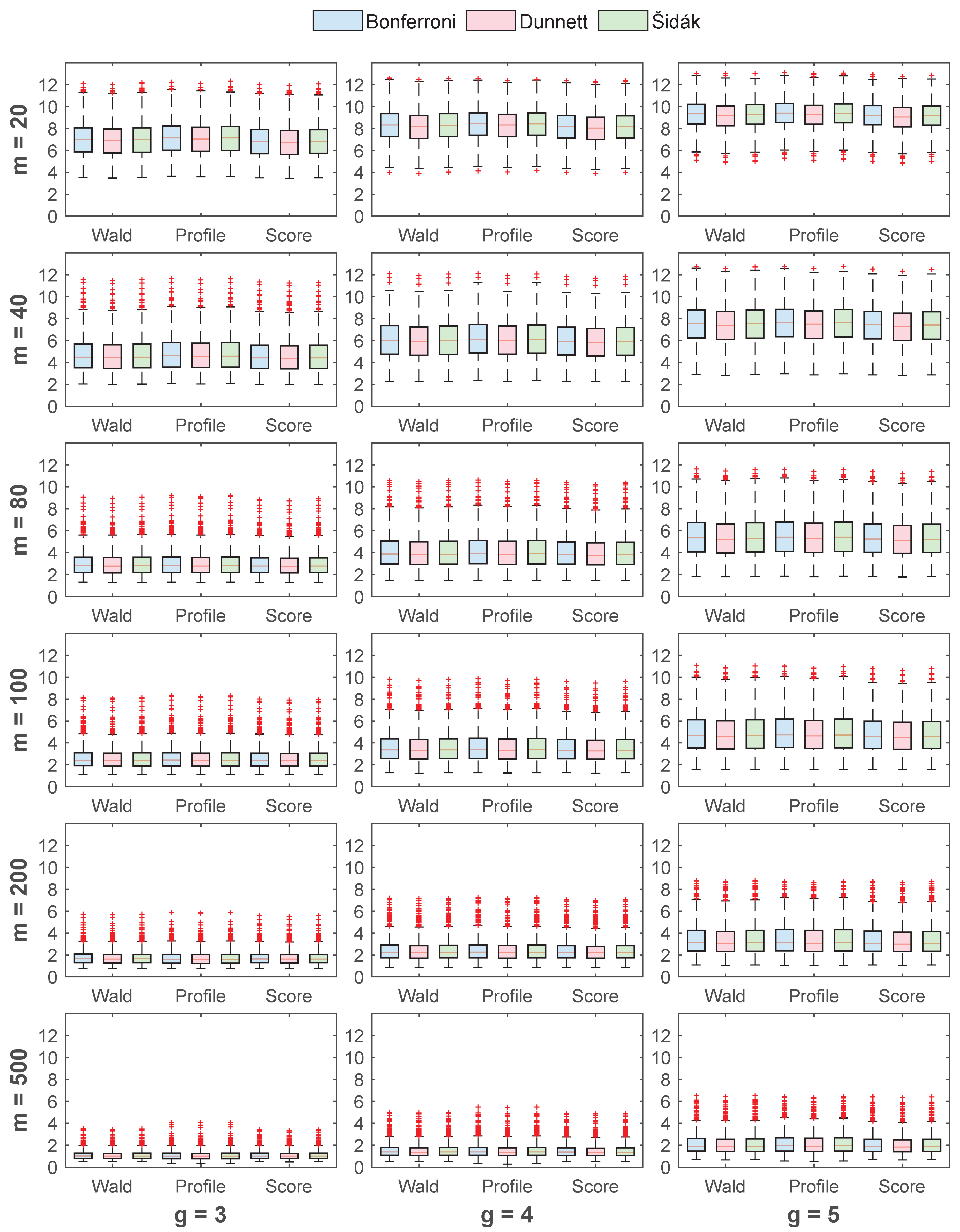
An additional simulation study was conducted for balanced designs with $g=$ 3, 4, and 5 groups and sample sizes $m=$ 20, 40, 80, 100, 200, and 500. For each configuration, 1000 parameter settings were independently generated from the uniform (0,1) distribution, subject to the constraints $\rho \in (0,1)$, ${\pi }_i\in (0.1,0.9)$, and the corresponding response probabilities are specified in Equation (1). The values of ${\pi }_i$ were chosen to avoid boundary values. The values of ${\pi }_i$ were arranged in an ascending order to ensure that the OR between the ith group $(i=2,\dots ,g)$ and the first group was greater than one. This ordering facilitated a more consistent comparison of MIWs across configurations.

For each parameter configuration, 10,000 replications were generated. The results of the SCIs were evaluated against the true OR values to derive the ECP and the MIW. The findings across all 1000 configurations were subsequently summarized and presented using box plots to provide a comprehensive visual assessment of the distributional behavior of each method.

The box plots in Figure 1 and Figure 2 illustrate the overall distributions of the ECP and MIW for all SCI methods considered. Combined with the previous simulation study, the score method with Dunnett multiplicity adjustment performed the best, achieving an average ECP closest to the prespecified nominal level and the shortest MIW.

Figure 1. Box plots of empirical coverage probabilities.

Figure 2. Box plots of mean interval width.

As shown in Figure 1, the Score–Dunnett method generally produced ECPs closest to the nominal level of 0.95 among the nine methods. The Profile–Dunnett method also showed comparable coverage, although larger interquartile ranges (IQRs) and more lower-tail outliers were observed in some settings. The Wald–Dunnett method provided relatively stable results, particularly when the number of groups was small, with narrower IQRs and fewer outliers. As the sample size increased, the ECP distributions generally became more concentrated around the nominal level, with smaller IQRs for most methods. This pattern was particularly noticeable when the number of groups was larger. However, the profile-based methods showed larger variation and more lower-tail outliers in some settings. The Bonferroni-adjusted methods generally produced ECPs above 0.95, especially at smaller sample sizes, indicating more conservative coverage than the corresponding Šidák- and Dunnett-adjusted methods.

Meanwhile, Figure 2 shows that the MIW decreased substantially as the sample size increased, while the distribution of MIW values became more concentrated, reflecting the improved performance of asymptotic methods with larger samples. In contrast, the MIW exhibited a slight increase as the number of groups increased. This occurred because the MIW was computed as the average width across all SCIs. In the simulation settings, the ${\pi }_i$ values were ordered in ascending order, and the ORs comparing group i ($i=2,\dots ,g$) with the first group were greater than one and increasing with i. Therefore, additional intervals corresponding to larger ORs were included in the calculation, resulting in a slightly larger MIW.

4. Real Case Example

In this paper, we reanalyze the data sourced from Rosner’s study [4] to illustrate the performance of the proposed simultaneous confidence interval methods. The data include 218 patients diagnosed with retinitis pigmentosa (RP) aged between 20 and 39 who received treatment at the Massachusetts Eye and Ear Infirmary from 1970 to 1979. Based on their genetic classification, patients were divided into four groups: autosomal dominant RP (DOM), autosomal recessive RP (AR), sex-linked RP (SL), and isolated RP (ISO). To simplify the analysis, each patient was associated with a single family unit, and individuals were randomly selected for the study. Each participating patient was required to provide visual acuity information for both eyes. Ocular status was determined according to the visual acuity measurements; an eye was considered affected by retinitis pigmentosa if its Snellen visual acuity (VA) was 20/50 or worse, and an eye was classified as having normal vision if its acuity was 20/40 or better. For this analysis, 216 individuals with complete binocular visual acuity records were selected from the original cohort of 218 patients. Detailed information is presented in Table 6.

Table 6. Number of affected eyes per person in each group.

	Genetic Type
Number of Affected Eyes	ISO	DOM	AR	SL
0	67	15	7	3
1	24	6	5	2
2	57	7	9	14

The goodness-of-fit test indicates that the $\rho$ model provided an adequate fit to these data [28,29], suggesting that the common-correlation assumption is reasonable for this application. According to Ma and Liu [7], the estimated values for the parameters were $\widehat{\rho }$ = 0.6416, $\widehat{{\pi }_{ISO}}$ = 0.4658, $\widehat{{\pi }_{DOM}}$ = 0.3625, $\widehat{{\pi }_{AR}}$ = 0.5455, and $\widehat{{\pi }_{SL}}$ = 0.7926. These are close to the true probability of each group: ${\pi }_{ISO}$ = 0.4662, ${\pi }_{DOM}$ = 0.3571, ${\pi }_{AR}$ = 0.5476, ${\pi }_{SL}$ = 0.7895. When calculating the SCI, ISO was considered the control group based on evidence suggesting that RP may occur as an isolated sporadic disorder without genetic links. The 95% SCI among DOM, AR, SL, and ISO are presented in Table 7. Confidence intervals are relatively straightforward to interpret and apply in statistical analysis. According to prior simulation results, the score method with Dunnett adjustment was identified as the most effective approach. Additionally, the Wald–Dunnett and Profile–Dunnett methods demonstrated competitive performance. Since the statistical inference was based on the OR, significance was assessed by determining whether the corresponding confidence interval included the value of one.

Table 7. 95% SCIs of the proportion ratio of affected rates among these groups.

	SCIs
Methods	DOM/ISO	AR/ISO	SL/ISO
Wald–Bonferroni	(0.259, 1.640)	(0.499, 3.800)	(1.240, 15.495)
Wald–Dunnett	(0.279, 1.522)	(0.541, 3.500)	(1.373, 13.987)
Wald–Šidák	(0.260, 1.636)	(0.500, 3.790)	(1.244, 15.445)
Profile–Bonferroni	(0.254, 1.594)	(0.506, 3.822)	(1.352, 18.393)
Profile–Dunnett	(0.275, 1.483)	(0.550, 3.508)	(1.481, 16.112)
Profile–Šidák	(0.255, 1.590)	(0.508, 3.811)	(1.356, 18.314)
Score–Bonferroni	(0.271, 1.577)	(0.526, 3.593)	(1.284, 14.773)
Score–Dunnett	(0.290, 1.470)	(0.568, 3.333)	(1.412, 13.496)
Score–Šidák	(0.271, 1.574)	(0.527, 3.585)	(1.288, 14.731)

The results show that the confidence intervals between DOM and ISO as well as AR and ISO contained one, indicating no significant difference between these groups. However, the lower bounds of the confidence intervals between the SL and ISO group were greater than one, indicating significantly higher odds of an eye being affected in the SL group than in the ISO group. Clinically, this finding is consistent with the more severe visual impairment generally reported for sex-linked RP, particularly in affected males. In contrast, isolated RP did not represent a single mode of inheritance, and it may comprise cases with heterogeneous underlying genetic causes. These differences may partly explain the higher proportion of affected eyes observed in the SL group [30].

5. Discussions

In this paper, nine asymptotic simultaneous confidence intervals (SCIs) were derived for the OR. These asymptotic procedures are based on large sample theory and are applicable when sample sizes are sufficiently large. However, they may produce unreliable coverage probabilities when sample sizes are small or sparse. In such cases, exact methods would be more appropriate, which could be considered for future analysis. In addition to small sample sizes, the accuracy of the asymptotic approximation may also be affected when the correlation coefficient $\rho$ approaches the boundary of its admissible parameter space. Therefore, caution is warranted when applying the proposed methods when $\rho$ is close to one. To control the Type I error rate, this study compared three multiplicity adjustment methods—the Bonferroni, Šidák, and Dunnett corrections—within the framework of the proposed SCIs. Among these, the Dunnett method showed the best performance. The Šidák correction showed a slightly better performance than the Bonferroni correction, while both methods involve relatively straightforward calculations. Exploring alternative multiplicity adjustment methods could be considered as a direction for future work. Another limitation of the proposed approach concerns computational efficiency. For the Dunnett method, the computation time increased moderately as the number of groups increased, mainly due to the root-finding procedure. For settings with a relatively large number of groups, further optimization of the computational algorithm may be considered to improve efficiency. Finally, the asymptotic SCIs proposed in this paper are designed for bilateral (two-sided) data. Extending the framework to incorporate both unilateral and bilateral data would broaden its applicability and represents an important direction for future work.

References

- Ying, G.S.; Maguire, M.G.; Glynn, R.; Rosner, B. Tutorial on biostatistics: Linear regression analysis of continuous correlated eye data. Ophthalmic Epidemiol. 2017, 24, 130–140. [Google Scholar] [CrossRef] [Scilit]
- Camarillo, N.D.; Jiménez-Silva, R.; Sheehan, F.T. Using bilateral data in controls and patients with bilateral and unilateral pathology requires increased scrutiny. J. Biomech. 2024, 162, 111855. [Google Scholar] [CrossRef] [Scilit]
- Liang, K.Y.; Zeger, S.L. Longitudinal data analysis using generalized linear models. Biometrika 1986, 73, 13–22. [Google Scholar] [CrossRef]
- Rosner, B. Statistical methods in ophthalmology: An adjustment for the intraclass correlation between eyes. Biometrics 1982, 38, 105–114. [Google Scholar] [CrossRef] [Scilit]
- Dallal, G.E. Paired bernoulli trials. Biometrics 1988, 44, 253–257. [Google Scholar] [CrossRef] [Scilit]
- Donner, A. Statistical methods in ophthalmology: An adjusted chi-square approach. Biometrics 1989, 45, 605–611. [Google Scholar] [CrossRef] [Scilit]
- Ma, C.X.; Liu, S. Testing equality of proportions for correlated binary data in ophthalmologic studies. J. Biopharm. Stat. 2017, 27, 611–619. [Google Scholar] [CrossRef] [Scilit]
- Liu, X.; Shan, G.; Tian, L.; Ma, C.X. Exact methods for testing homogeneity of proportions for multiple groups of paired binary data. Commun. Stat.—Simul. Comput. 2017, 46, 6074–6082. [Google Scholar] [CrossRef] [Scilit]
- Newcombe, R.G. Improved confidence intervals for the difference between binomial proportions based on paired data. Stat. Med. 1998, 17, 2635–2650. [Google Scholar] [CrossRef] [Scilit]
- Tang, M.L.; Ling, M.H.; Ling, L.; Tian, G. Confidence intervals for a difference between proportions based on paired data. Stat. Med. 2010, 29, 86–96. [Google Scholar] [CrossRef] [Scilit]
- Pei, Y.; Tang, M.L.; Wong, W.K.; Guo, J. Confidence intervals for correlated proportion differences from paired data in a two-arm randomised clinical trial. Stat. Methods Med. Res. 2012, 21, 167–187. [Google Scholar] [CrossRef] [Scilit]
- Tang, M.L.; He, X.; Tian, G. A confidence interval approach for comparative studies involving binary outcomes in paired organs. Commun. Stat.—Simul. Comput. 2013, 42, 425–453. [Google Scholar] [CrossRef] [Scilit]
- Newcombe, R.G. Confidence intervals for the mean of a variable taking the values 0, 1 and 2. Stat. Med. 2003, 22, 2737–2750. [Google Scholar] [CrossRef] [Scilit]
- Pei, Y. Statistical Inference for Correlated Binary Data from Bilateral Studies. Doctoral Thesis, Hong Kong Bapist University, Hong Kong, China, 2009. [Google Scholar]
- Tang, N.S.; Li, H.Q.; Tang, M.L.; Li, J. Confidence interval construction for the difference between two correlated proportions with missing observations. J. Biopharm. Stat. 2016, 26, 323–338. [Google Scholar] [CrossRef] [Scilit]
- Document Guidance. Master Protocols: Efficient Clinical Trial Design Strategies to Expedite Development of Oncology Drugs and Biologics Guidance for Industry. Guidance for Industry; FDA: Silver Spring, MD, USA, 2022. Available online: https://fda.gov/media/120721/download (accessed on 1 March 2022).
- Peng, X.; Liu, C.; Liu, S.; Ma, C.X. Asymptotic confidence interval construction for proportion ratio based on correlated paired data. J. Biopharm. Stat. 2019, 29, 1137–1152. [Google Scholar] [CrossRef] [Scilit]
- Yang, Z.; Tian, G.L.; Liu, X.; Ma, C.X. Simultaneous confidence interval construction for many-to-one comparisons of proportion differences based on correlated paired data. J. Appl. Stat. 2020, 48, 1442–1456. [Google Scholar] [CrossRef] [Scilit]
- Yang, Z. Confidence Interval Construction for the Difference of Proportions Based on Correlated Bilateral Data. Doctoral Dissertation, University at Buffalo, Buffalo and Amherst, NY, USA, 2017. [Google Scholar]
- National Academies of Sciences Engineering, and Medicine. Reference Manual on Scientific Evidence, 4th ed.; National Academies Press (US): Washington, DC, USA, 2025. [Google Scholar]
- Kestenbaum, B. Epidemiology and Biostatistics: An Introduction to Clinical Research; Springer: Cham, Switzerland, 2009; ProQuest Ebook Central. [Google Scholar]
- Newcombe, R.G. Confidence Intervals for Proportions and Related Measures of Effect Size; CRC Press: Boca Raton, FL, USA, 2012. [Google Scholar]
- Zbyněk, Šidák. Rectangular confidence regions for the means of multivariate normal distributions. J. Am. Stat. Assoc. 1967, 62, 626–633. [Google Scholar] [CrossRef] [Scilit]
- Dunnett, C.W. A Multiple Comparison Procedure for Comparing Several Treatments with a Control. J. Am. Stat. Assoc. 1955, 50, 1096–1121. [Google Scholar] [CrossRef] [Scilit]
- Piegorsch, W.W. Multiple comparisons for analyzing dichotomous response. Int. Biom. Soc. 1991, 47, 45–52. [Google Scholar] [CrossRef] [Scilit]
- Tang, M.L.; Tang, N.S.; Rosner, B. Statistical inference for correlated data in ophthalmologic studies. Stat. Med. 2006, 25, 2771–2783. [Google Scholar] [CrossRef] [Scilit]
- Tang, N.S.; Tang, M.L.; Qiu, S.F. Testing the equality of proportions for correlated otolaryngologic data. Comput. Stat. Data Anal. 2008, 52, 3719–3729. [Google Scholar] [CrossRef] [Scilit]
- Liu, X.; Ma, C.X. Goodness-of-fit tests for correlated bilateral data from multiple groups. In Contemporary Experimental Design, Multivariate Analysis and Data Mining; Springer: Berlin/Heidelberg, Germany, 2020; pp. 311–327. [Google Scholar]
- Zhou, J.; Ma, C.X. Goodness-of-fit tests for combined unilateral and bilateral data. Mathematics 2025, 13, 2501. [Google Scholar] [CrossRef] [Scilit]
- Fahim, A.T.; Daiger, S.P.; Weleber, R.G. Nonsyndromic retinitis pigmentosa overview. In GeneReviews® [Internet]; University of Washington: Seattle, WA, USA, 2000. [Google Scholar]
Disclaimer/Publisher’s Note: The statements, opinions and data contained in all publications are solely those of the individual author(s) and contributor(s) and not of MDPI and/or the editor(s). MDPI and/or the editor(s) disclaim responsibility for any injury to people or property resulting from any ideas, methods, instructions or products referred to in the content. |
© 2026 by the authors. Licensee MDPI, Basel, Switzerland. This article is an open access article distributed under the terms and conditions of the Creative Commons Attribution (CC BY) license.