Abstract
This paper explores a numerical method for European and American option pricing under time fractional jump-diffusion model in Caputo scene. The pricing problem for European options is formulated using a time fractional partial integro-differential equation, whereas the pricing of American options is described by a linear complementarity problem. For European option, we present nonuniform discretization along time and the radial basis function (RBF) method for spatial discretization. The stability and convergence analysis of the discrete scheme are carried out in the case of European options. For American option, the operator splitting method is adopted which split linear complementary problem into two simple equations. The numerical results confirm the accuracy of the proposed method.
Keywords:
Caputo fractional derivative; time fractional Black-Scholes model; jump-diffusion model; option pricing; RBF method; graded meshes MSC:
35R09; 35R11; 65M12; 65M22
1. Introduction
Option pricing refers to the process of calculating and determining the price of option contracts based on specific financial models and market conditions. Option pricing plays an important role in financial markets, not only helping investors manage risks and make investment decisions, but also promoting effective market operation and reasonable asset pricing. The famous option pricing model is Black-Scholes (BS) model, which was proposed by Black and Scholes [1] in 1973. The model is based on the assumption of a log normal distribution of stock prices, which considered the relationship between option prices and underlying asset prices, strike prices, risk-free interest rates, option expiration times, and underlying asset volatility. However, the strict assumptions of the BS model often do not hold true in the actual market. To overcome this problem, many improved models have been put forward, such as stochastic volatility models, jump-diffusion models, fractional BS models, etc. The improvement and research of stochastic models can be found in [2,3]. The paper mainly focuses on the jump-diffusion model and fractional BS model.
Merton [4] and Kou [5] considered jump-diffusion models, assuming that the underlying asset price follows a jump-diffusion with a normal distribution and the jump size has a double exponential distribution, respectively. Due to its ability to accurately reflect the volatility observed in real markets, the jump-diffusion model has been widely applied in financial markets. For the jump-diffusion models, numerical methods are usually used to solve the partial integro-differential equations (PIDEs) that the option prices satisfy. Toivanen [6] used finite difference (FD) discrete space differential operators on non-uniform grids and performed time discretization using implicit Rannacher schemes. For the calculation of integral terms, an recursive formula has been derived. Salmi and Toivanen [7] raised a family of IMEX discretization schemes for PIDEs, Christara and Leung [8] demonstrated that the combination of quadratic spline collocation method and Picard iteration scheme can efficiently solve the pricing problem. Rad and Parand [9] proposed the local weak form meshless methods for jump-diffusion pricing models. Kwon and Lee [10] adopted the implicit FD method incorporating operator splitting method to solve the linear complementarity problems (LCPs) that American option satisfied. Saib et al. [11] and Chan and Hubbert [12] proposed the radial basis functions (RBF) method, and Haghi et al. [13] combined the RBF method with IMEX scheme for option pricing.
In 1997, Carpinterj and Mainardi [14] emphasized the practicality of fractional partial differential equations (FPDEs) in researching fractal geometry and dynamics, and then FPDEs are gradually integrated into financial theory. Wyss [15] and Chen et al. [16] proposed different time fractional BS equations (FBSEs) for option pricing. Subsequently, it is extended to more general situations, for example, the interest rate and volatility are functions of the underlying asset price and time [17,18]. Important issues that urgently need to be addressed is the solutions of time FBSEs. The analytical solutions obtained through integral transformation methods often involve the integral form of special functions, making them difficult to calculate [15]. However, methods such as homotopy perturbation method [19,20], homotopy analysis method [21,22], RPSM [23], and ADM [24] are widely used to solve FBSEs and get series solutions due to their independence from discretization and linearization.
Due to the dependence of analytical solutions on some special functions or convolutions of infinite series and integrals, it has become very important to study numerical methods for solving the option pricing problem controlled by FPDE. Song and Wang [25], and Koleva and Vulkov [26] proposed an implicit FD method for put option pricing and weighted FD under the Jumarie [27] model, respectively. Yang et al. [28] used the FD method to solve the time-space FBSEs. Zhang et al. [29] derived a numerical solution of barrier options in a time FBSEs. Cen et al. [30] transformed differential equations into integral form, discretized them on adaptive grids, and proved the convergence. Rahimkhani et al. [31] presented a new numerical method based on Hahn hybrid functions for solving of BS option pricing distributed order time FPDE. Maddouri [32] proposed a new -Caputo fractional BS model which was solved by numerical implicit scheme, as well as the stability and convergence were studied.
In order to improve the accuracy, compact scheme and high-order time discretization techniques are adopted. Staelen and Hendy [33] designed a compact spatial fourth-order difference scheme. Abdi et al. [34] fused the L1-2 format with the sixth and eighth order compact schemes to obtain two high-order numerical methods. References [35,36] also employed compact schemes and high-order time discretization methods. Another popular meshless method is RBF. Nikan et al. [37] solved the time FBSE using local RBF method instead of global RBF method. Delpasand and Hosseini [38] extended the global RBF method to approximate the option pricing models under two types of assets, using the L1 scheme based C-N method to discretize time variables. In addition, to address the issue of reduced convergence order observed under initial conditions with non-smoothness, a modified L1 scheme [39] and various RBFs [40,41] are adopted.
Mohapatra et al. [42] considered a time FBSE under jump-diffusion model. A graded mesh combined with the FD scheme were adopted to derive a completely discrete framework. Chen and Li [43] developed an IMEX compact FD scheme to solve the time fractional partial integro-differential equations (TFPIDEs). To our knowledge, there are few literature studies on the pricing of options under time fractional jump-diffusion models, especially for American options. In this work, the main objective is to investigate numerical methods for evaluating the option prices under a time fractional jump-diffusion model, including European and American options. For simplicity of the analysis, the European options pricing can be transformed into a TFPIDE with a Fredholm integral operator, which is solved by using a discrete scheme of non-uniform fractional discretization along time and spatial discretization using RBF method, as well as composite trapezoidal approximation for Fredholm operator, while American options can be described by LCP, which is decomposed into two simple equations using operator splitting method. Stability and convergence analysis are discussed, and the optimal convergence rate is shown for graded meshes.
The paper is organized as follows. Section 2 introduces some preliminary knowledge about fractional integrals and fractional derivatives. In Section 3, the pricing model of European and American options are presented under time fractional jump-diffusion model. Section 4 introduces the discrete scheme and operator splitting method of European and American options. Section 5 demonstrates the stability and convergence of the discretization method. Section 6 conducted numerical experiments and empirical analysis, and the experimental results verified our expectations. Section 7 is the conclusion.
2. Preliminaries
This section introduces some basic definitions and preliminary knowledge about fractional integrals and fractional derivatives, as well as some well-known properties [44].
Definition 1.
Let be continuous. The Riemann–Liouville fractional integral of the function is defined by:
where , the set of all positive real numbers, be the order of the integral.
Definition 2.
The Caputo fractional derivative of the function is defined by:
where is the order of the derivative and , the smallest integer which is greater than or equal to δ.
Some properties of fractional integrals and derivatives are given as follows.
- For any constant function (c is a constant) .
- For any , we have
- For , we have , but .
- Fractional integrals and derivatives satisfy the linearity property:
- (a)
- (b)
are some positive constants.
3. Option Pricing Model
Assume the stock price is controlled by the following equation
where and denote the standard Brownian motion and the independent Poisson process with intensity , respectively. is an impulse function producing a jump from to , represents the expected value of jump size distribution under Merton model, and
is the density function of log-normal distribution. The density function for all z, and meet , which is defined by
In addition, and signify the mean and variance of jumps, respectively, and parameters , and represent risk-free interest rates, dividends, and volatility, respectively.
3.1. TFPIDE for European Option
Under the jump-diffusion model, European option price at time and stock price S with strike price K and expiry date T satisfies the following TFPIDE
where is Caputo’s fractional derivative which is given by
For European call option, the conditions of boundary and payoff function are given as
and for European put option, the conditions of boundary and payoff function are given as
Set , and , the problem (2) is converted into a TFPIDE with a Fredholm integral operator. We have
To apply numerical approximation, we limit the range of spatial variables to a bounded interval, considering the bounded domain instead of the domain . Let , , , and , we have
where
and .
3.2. LCP for American Option
Let be the American put option price with strike price K and expiry date T under the jump-diffusion model which satisfies the following LCP
where the conditions of boundary and payoff function are given as
Similar to the handling of European options, by replacing the same variables, we obtain
4. The Discrete Problem
To construct the numerical solution of TFPIDE, we apply the local RBF method in spatial and graded meshes in time.
4.1. Nonuniform Fractional Discretization along Time
Due to the non-smooth of TFPIDE at , it also leads to inaccuracy at and , we consider a well-known graded temporal partition. Let
where , and is the grading parameter that controls the density of the points. When , the points is equidistant. The step size is At each nodes , , we have
For the nonuniform nodes, the L1 discretization is used on graded meshes which obtains the following scheme
where , . A short calculation using the mean value theorem revealed that
and
which can be found in [42,45].
4.2. Spatial Discretization
In this part, we explain the spatial discretization of the local RBF method, which is considered as an extension of the classical FD method and is referred to as RBF-FD. Polynomial interpolation is used to calculate weights for the FD method, while RBF interpolation is calculated by fitting grid points and some adjacent points in the RBF-FD method. RBF-FD method is a local RBF method which can overcome the ill-conditioning of the linear system, while the global RBF method considers all grid points to determine interpolation coefficients, which can lead to ill-conditioning in dense linear systems.
Consider a finite set consisting of M scattered nodes , and a differential operator . For a given node , the goal is to approximate as a linear combination of U at the M scattered nodes, so that
A set of base function are required for determining the RBF-FD weights , and
By solving a linear simultaneous equations, weight coefficients are obtained. Next, we will adopt multiquadrics as RBFs
where c is the shape parameter, which controls the shape of RBF. The accuracy of RBF method highly depends upon the shape parameter c of the basis functions, which is responsible for the flatness of the functions.
Now, we demonstrate how to get accurate RBF-FD formulas in one-dimensional cases of our model. Define nodes in the interval such that , , where . The boundary nodes are and . We mainly focus on internal nodes , . Selecting multiquadric function
as RBF, and using three equally spaced nodes, it holds that
Assuming , using Taylor expansion and omitting higher-order terms, as in [13,41], one yields
Let , and , hence
4.3. Discretization of the Integral Operator
Under the spatial and time discretization,
holds. The integration is approached by the composite trapezoidal rule, and requires the use of the th level solution to approximate the jth level solution, therefore
where for , and for .
According to Equations (6)–(8), we get a discretization scheme for European options on a non-uniform grid
where
Neglecting and denoting as the approximate soluton at each , we have
By organizing, it can be concluded that
where
For American options, we adopt operator splitting method for solving the LCP. An auxiliary function is introduced for the LCP, and the LCP (5) can be transformed to
Operator splitting method splits the Equation (12) into two subproblems by using intermediate solution . In the first step, solving by the following equation
and in the second step, we solve by
The solution of (14) is
5. Stability and Convergence Analysis
This section discusses the stability and convergence of the discrete scheme (11), and the stability multipliers are taken into account to show the convergence results.
5.1. Stability Analysis
Lemma 1.
The solution of Equation (11) satisfies
Proof.
By transferring items to Equation (11) and organizing them, it can be obtained that
Define
For a fixed , there exists such that holds. Therefore, at each grid node , there are
where
Due to being established, and based on the selection of , there are
which can be inferred as
□
Define the real numbers for and by
Theorem 1.
For , the solution of Equation (11) satisfies
Proof.
Using mathematical induction for proof. For , we have
which can be obtained by Lemma 1.
Assuming for and , Theorem 1 holds. Then for , we get
□
5.2. Convergence Analysis
To demonstrate the convergence, we first calculated the truncation error bound at points . Then, using the stability results, the complete error bound of the proposed method was established.
Let , where and denote the exact solution and numerical solution at node , respectively. Then, we get
According to the discretization on time, space and integration, the remaining term consists of four parts. The first remaining term satisfies
The second and third remaining terms satisfy
The remaining terms in part four are caused by the composite trapezoidal formula and the approximation of the th layer solution instead of the jth layer solution. The latter will result in errors that depend on the grading parameters such that . According to [45], we have
Hence, the infinite norm of the remainder in the fourth part is less than or equal to
To obtain the convergence theorem for numerical formats, we first provide the following lemma.
Lemma 2.
When parameter , for , one has
Proof.
Use induction on j, the Lemma is proved [45]. □
Theorem 2.
The error bounds of the discretization scheme (11) satisfy
Proof.
According to Theorem 1, there is
Let , and according to Lemma 2,
Especially, if , we have
□
6. Numerical Experiments and Empirical Analysis
6.1. Numerical Experiments
We provide some numerical examples to illustrate the effectiveness of numerical methods. Theoretical analysis also holds true for the TFPIDE of the source term. For the completeness of the numerical experiment, we added source terms to the equation. All the results are calculated by using the mathematical software MATLAB R2023b. The algorithm is given as follows.
Step 1. Give the initial parameters .
Step 3. Calculate , and Coefficients in discrete scheme (11).
Step 4. Compute the coefficient matrix of the linear equation system composed of the coefficients in (11).
Step 5. Calculate the right-hand term of the linear equations system based on the expression of .
Step 6. Solve systems of linear Equation (11).
Example 1.
Consider the TFPIDE with nonhomogeneous boundary conditions
The exact solution of (19) is
The parameters values are , , , , , , and .
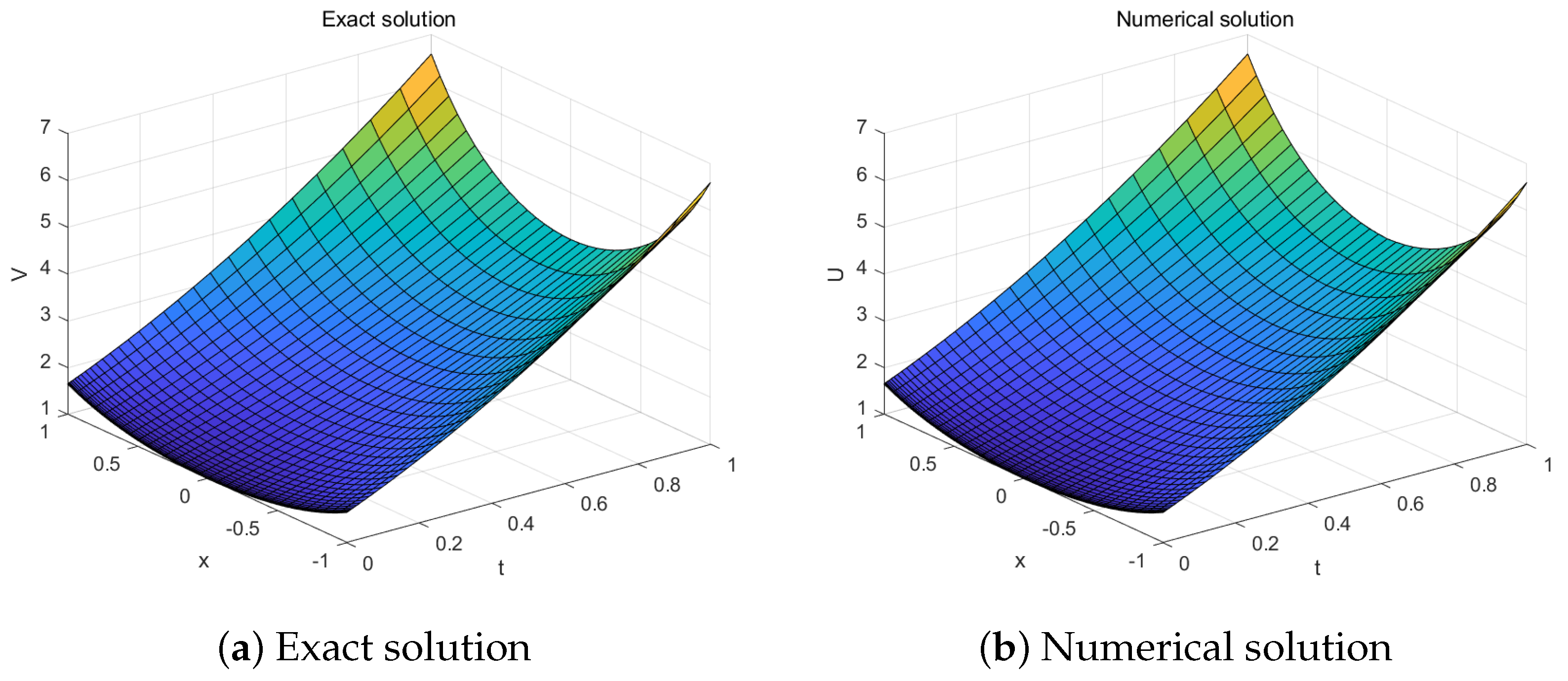
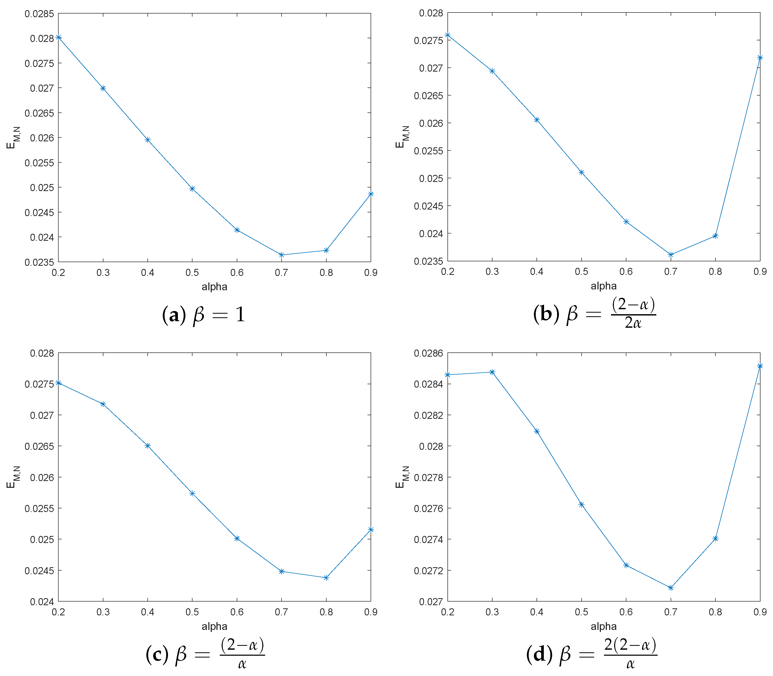
Figure 1 presents the exact solution and numerical solution with for and . Table 1 shows the comparison of solutions at some grid node, and the errors are also given. Figure 2 gives the maximum error for different and , where . Here, let , , , and in Figure 2a–d, respectively. The maximum error is defined by . From Figure 2, it can be seen that with the change of , the length of the interval for the maximum error change at and are smaller than and . Numerical errors and convergence orders are given by Table 2 for different , M and N with . The numerical errors are computed by mean squared error. The convergence order is computed by
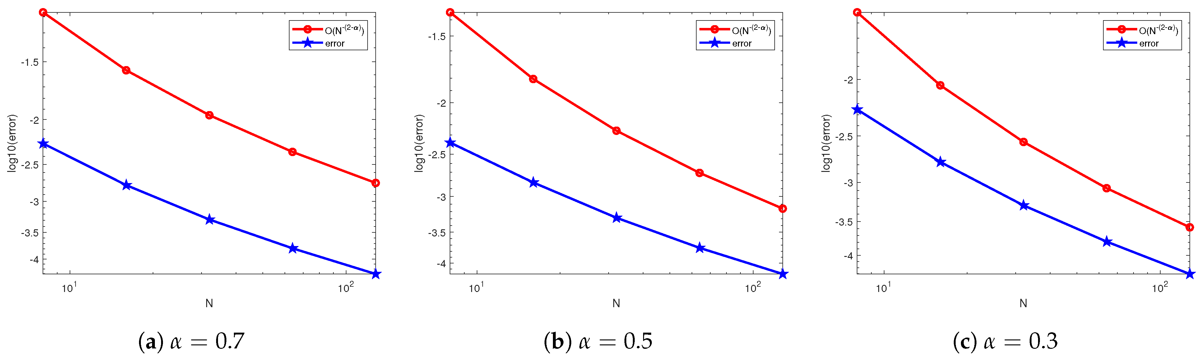
The log-log plots of the errors and the error bounds are shown in Figure 3 for different values of . It is observed that the convergence rate is when , which is the optimal rate.

Figure 1.
Exact solution and numerical solution with .

Table 1.
Comparison of solutions at some grid node.
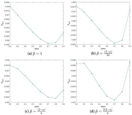
Figure 2.
Error for different and .
Table 2.
Numerical error, convergence orders, and CPU times.
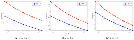
Figure 3.
against N for different .
Example 2.
Consider the TFPIDE of European options with parameters , and . The grading parameter , and .
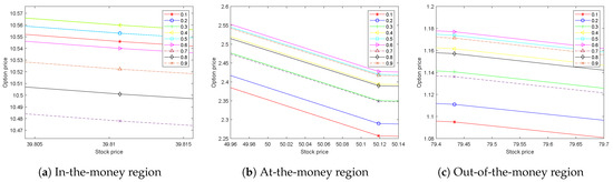
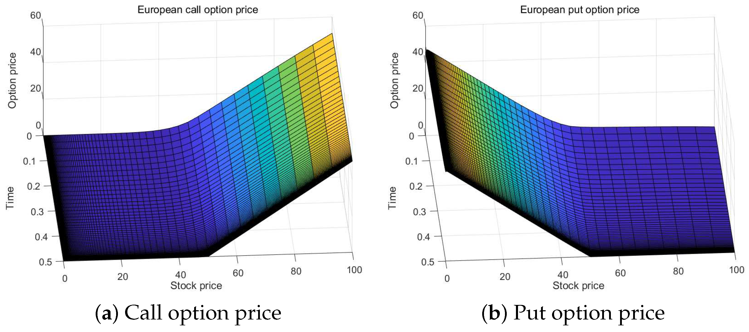
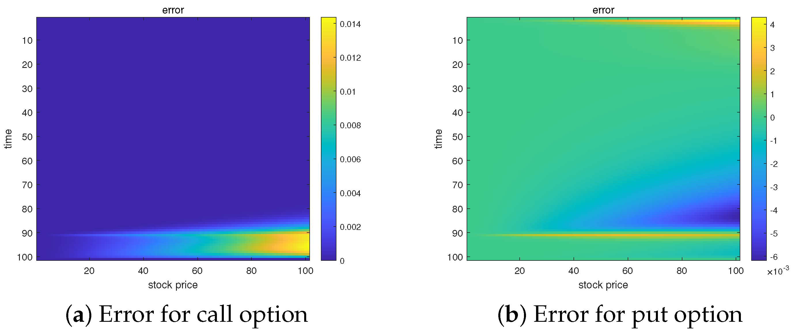
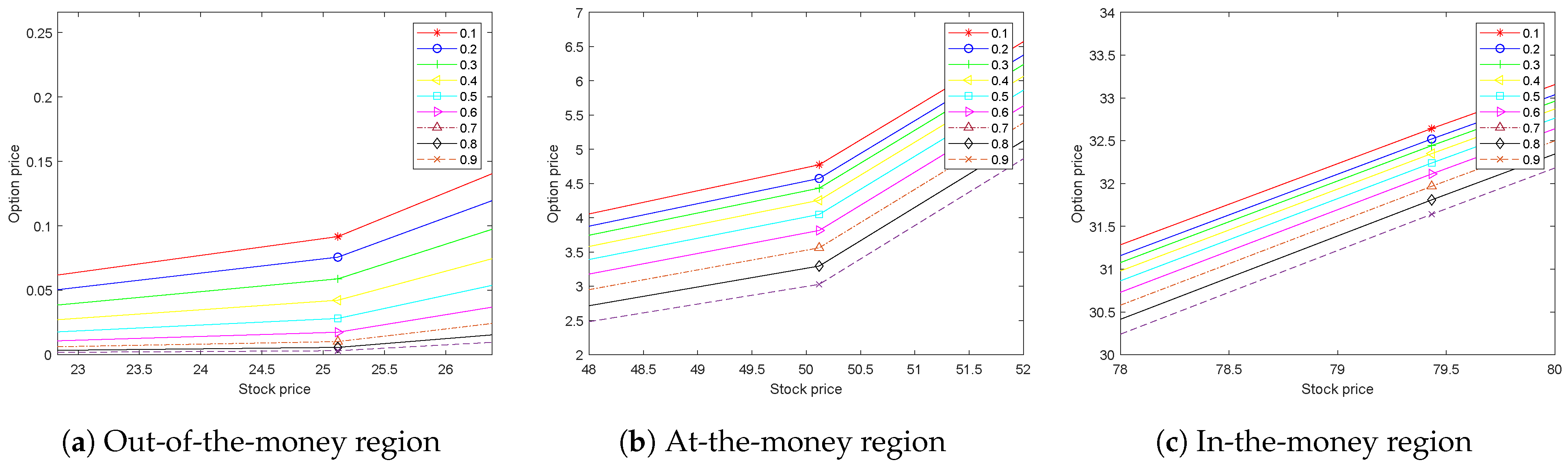
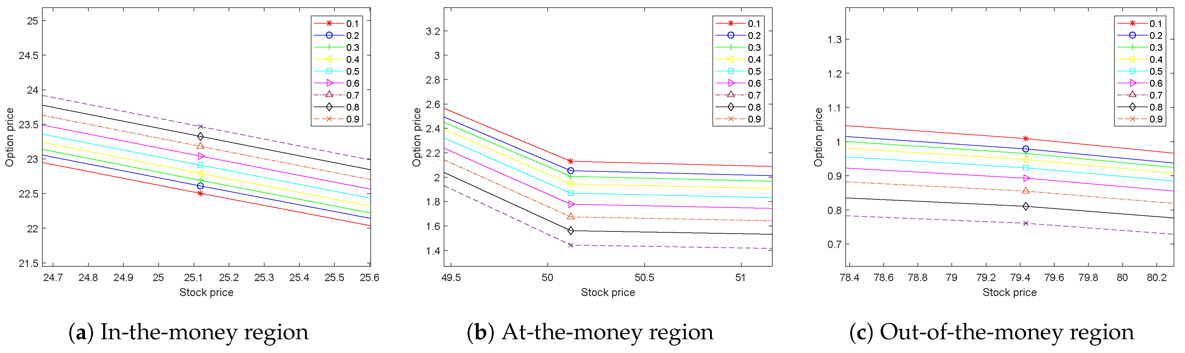
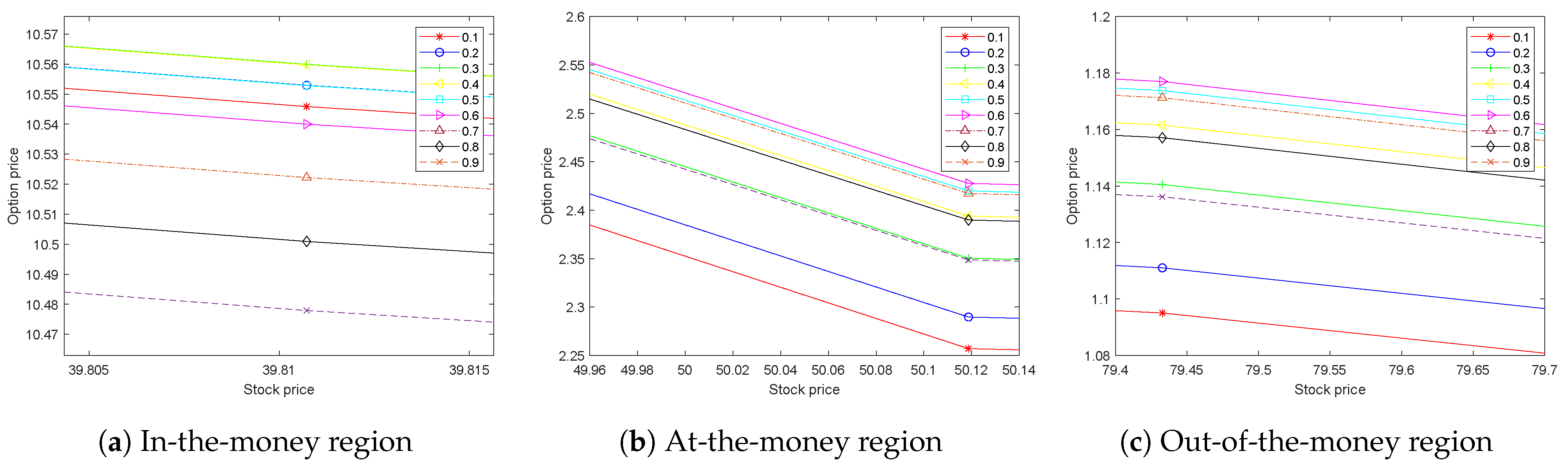
Figure 4 shows the European call and put option price using the proposed RBF method with . Due to the difficulty in obtaining option prices, we use the results obtained from the FD method as a benchmark to verify the effectiveness of our method. Figure 5 gives the European call and put option price using FD method. Figure 6a indicates that the error in calculating European call options using two methods ranges from 0 to 0.014, while Figure 6b indicates that the error in calculating European put options using both methods ranges from to . Figure 7 and Figure 8 display the numerical solution of the European call and put options for different and stock price. In Figure 7a, Figure 7b and Figure 7c, the curves from top to bottom correspond to , respectively. From these figures, it can be seen that for in-the-money, at-the-money, and out-of-the-money options, the option price decreases with the increase of for European call options. This behavior is similar to the effect of fractional parameters on fluid temperature. By increasing the value of fractional parameter , temperature profile decreases for small time t, thermal conductivity decreases [46]. Similar results can be obtained from Figure 8b,c for European put options. But according to Figure 8a, it can be seen that the price increases with the increase of for European put in-the-money options.

Figure 4.
European call and put option price using RBF method with .

Figure 5.
European call and put option price using FD method with .

Figure 6.
The error between RBF method and FD method for European call and put option.
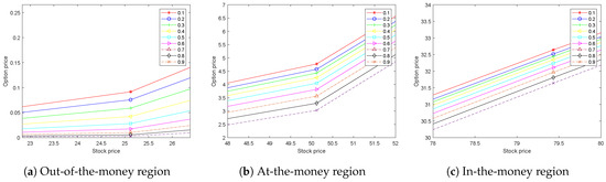
Figure 7.
European call option prices for different and stock price.
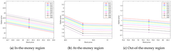
Figure 8.
European put option prices for different and stock price.
Example 3.

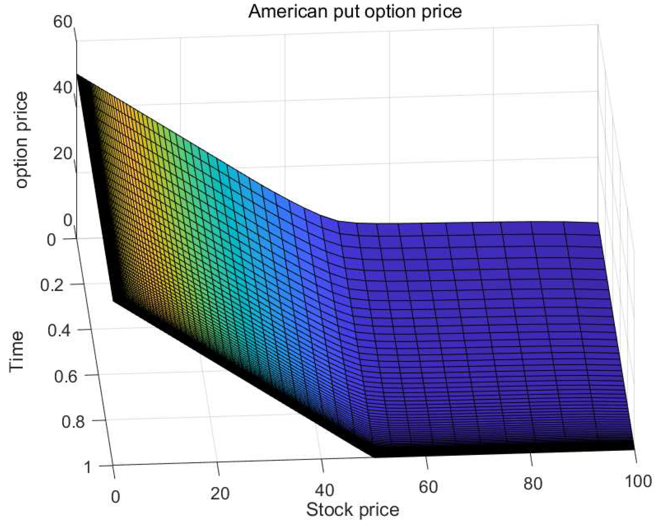
Consider the LCP of American put option with parameters , and . The grading parameter , and . Figure 9 shows the American put options for different time and stock price with . From Figure 10, it can be seen how time fractional derivative α affects the prices of American options.
Figure 9.
American put option price with .
Figure 10.
American option prices for different and stock price.
6.2. Empirical Analysis
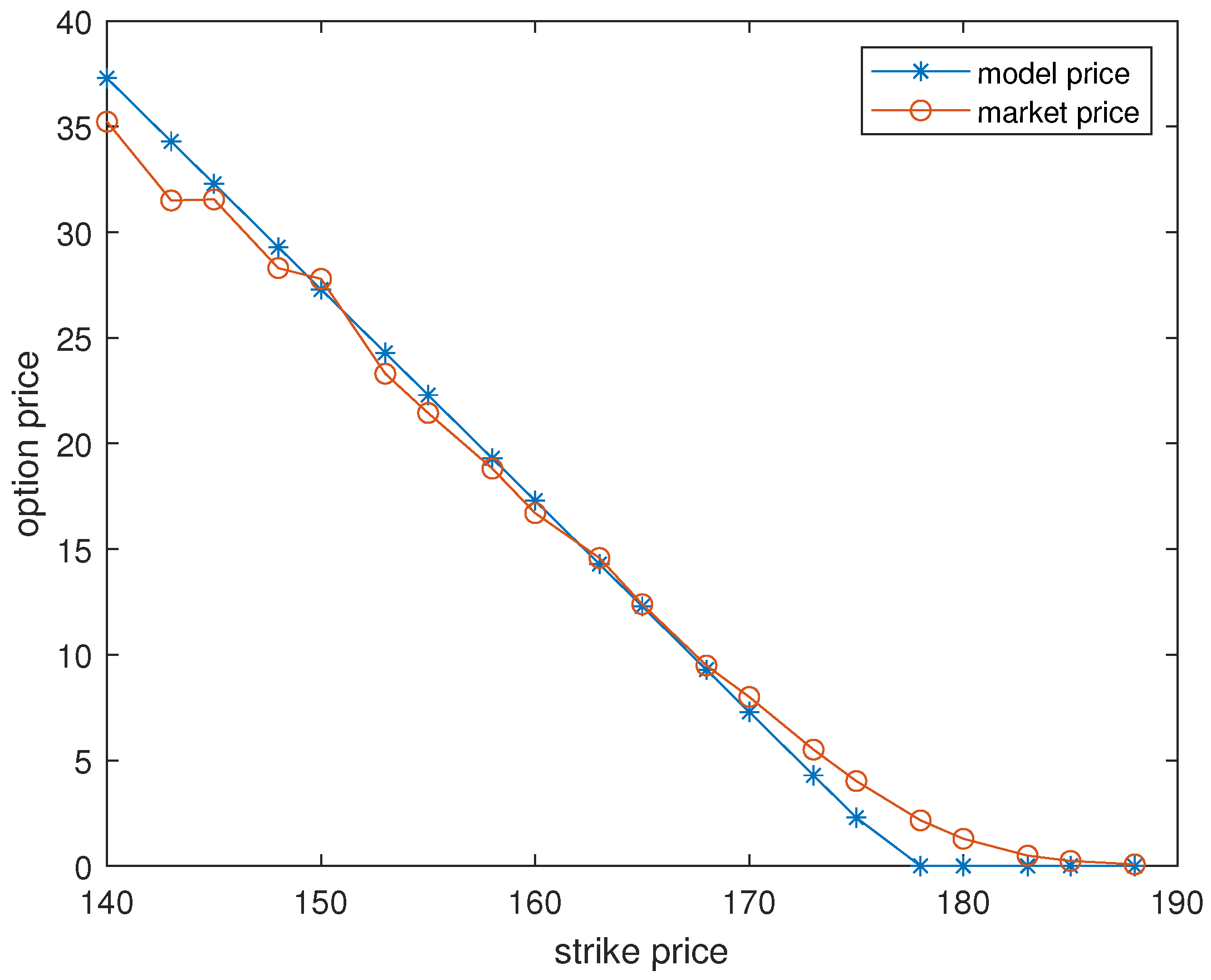
We select Standard & Poor Depositary Receipt (SPDR) option data from 8 November 2013 to 12 December 2013 for empirical analysis. Analyzing the historical closing prices of SPDR from 31 January 2011 to 8 November 2013, we give parameters as follows , . Figure 11 shows that our calculation results have a small error compared to real market data, while Table 3 shows that the error of the proposed method is smaller compared to the FD method, and the difference in CPU time occupied is also smaller, which indicate that we have indeed provided a truly effective method.
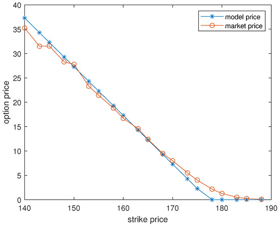
Figure 11.
American put option price with .
Table 3.
Error and CPU time of RBF and FD method.
7. Conclusions
In this paper, a new numerical method is put forward to solve the pricing problem of options in time fractional jump-diffusion models. The pricing problem of European option is represented as a TFPIDE, while American option is expressed as a LCP. For European option, nonuniform discretization along time and RBF method for spatial discretization are adopted. For American options, the operator splitting method is used to decompose LCP into two sub problems that are easy to solve numerically, namely linear boundary value problem and algebraic system. Stability and convergence rate are given, and the convergence rate is when . The numerical results are consistent with the theoretical results and demonstrate the impact of on option prices. The method is also applicable to the Kou model and can be extended to pricing singular options.
Author Contributions
W.G.: Conceptualization, methodology, software, validation, writing—original draft preparation, writing—review and editing, funding acquisition; Z.X.: Conceptualization, methodology, writing—review and editing, funding acquisition; Y.S.: software, writing—review and editing, supervision. All authors have read and agreed to the published version of the manuscript.
Funding
The work is supported by Shandong Provincial Natural Science Foundation (ZR2022QA055) and National Natural Science Foundation of China (62403156, 12071479).
Data Availability Statement
Data are contained within the article.
Acknowledgments
The authors thank the referees for their comments and detailed suggestions. These have significantly improved the presentation of the paper.
Conflicts of Interest
The authors declare no conflicts of interest.
References
- Black, F.; Scholes, M. The pricing of options and corporate liabilities. J. Polit. Econ. 1973, 81, 637–654. [Google Scholar] [CrossRef]
- TunÇ, O.; TunÇ, C. On the asymptotic stability of solutions of stochastic differential delay equations of second order. J. Taibah Univ. Sci. 2019, 13, 875–882. [Google Scholar] [CrossRef]
- Zouine, A.; Imzegouan, C.; Bouzahir, H.; Tunç, C. General decay stability of nonlinear delayed hybrid stochastic system with switched noises. Appl. Set-Valued Anal. Opt. 2024, 6, 157–177. [Google Scholar]
- Merton, R.C. Option pricing when underlying stock returns are discontinuous. J. Financ. Econ. 1976, 3, 125–144. [Google Scholar] [CrossRef]
- Kou, S.G. A jump-diffusion model for option pricing. Manag. Sci. 2002, 48, 1086–1101. [Google Scholar] [CrossRef]
- Toivanen, J. Numerical valuation of European and American options under Kou’s jump-diffusion model. SIAM J. Sci. Comput. 2008, 30, 1949–1970. [Google Scholar] [CrossRef]
- Salmi, S.; Toivanen, J. IMEX schemes for pricing options under jump-diffusion models. Appl. Numer. Math. 2014, 84, 33–45. [Google Scholar] [CrossRef]
- Christara, C.C.; Leung, N.C.-H. Option pricing in jump diffusion models with quadratic spline collocation. Appl. Math. Comput. 2016, 279, 28–42. [Google Scholar]
- Rad, J.A.; Parand, K. Pricing American options under jump-diffusion models using local weak form meshless techniques. Int. J. Comput. Math. 2017, 94, 1694–1718. [Google Scholar]
- Kwon, Y.; Lee, Y. A second-order tridiagonal method for American options under jump-diffusion models. SIAM J. Sci. Comput. 2011, 33, 1860–1872. [Google Scholar] [CrossRef]
- Saib, A.A.E.F.; Tangman, D.Y.; Bhuruth, M. A new radial basis functions method for pricing American options under Merton’s jump-diffusion model. Int. J. Comput. Math. 2012, 89, 1164–1185. [Google Scholar] [CrossRef]
- Chan, R.T.L.; Hubbert, S. Options pricing under the one-dimensional jump-diffusion model using the radial basis function interpolation scheme. Rev. Deriv. Res. 2014, 17, 161–189. [Google Scholar] [CrossRef]
- Haghi, M.; Mollapourasl, R.; Vanmaele, M. An RBF-FD method for pricing American options under jump-diffusion models. Comput. Math. Appl. 2018, 76, 2434–2459. [Google Scholar] [CrossRef]
- Carpinterj, A.; Mainardi, F. Fractals and Fractional Calculus in Continuum Mechanics; Springer: New York, NY, USA, 1997. [Google Scholar]
- Wyss, W. The fractional Black-Scholes equations. Fract. Calc. Appl. Anal. 2000, 3, 51–61. [Google Scholar]
- Chen, W.; Xu, X.; Zhu, S. Analytically pricing double barrier options based on a time-fractional Black-Scholes equation. Comput. Math. Appl. 2015, 69, 1407–1419. [Google Scholar] [CrossRef]
- Huang, J.; Cen, Z.; Zhao, J. An adaptive moving mesh method for a time-fractional Black-Scholes equation. Adv. Differ. Equ. 2019, 1, 516. [Google Scholar] [CrossRef]
- Rezaei, M.; Yazdanian, A.R.; Ashrafi, A.; Mahmoudi, S.M. Numerical pricing based on fractional Black-Scholes equation with time-dependent parameters under CEV model: Double barrier options. Comput. Math. Appl. 2021, 90, 104–111. [Google Scholar] [CrossRef]
- Elbeleze, A.A.; Kılıçman, A.; Taib, B.M. Homotopy perturbation method for fractional Black-Scholes European option pricing equations using Sumudu transform. Math. Probl. Eng. 2013, 2013, 524852. [Google Scholar] [CrossRef]
- Prathumwan, D.; Trachoo, K. On the solution of two-dimensional fractional Black-Scholes equation for European put option. Adv. Differ. Equ. 2020, 2020, 146. [Google Scholar] [CrossRef]
- Yavuz, M.; Özdemir, N. European Vanilla Option Pricing Model of Fractional Order without Singular Kernel. Fractal Fract. 2018, 2, 3. [Google Scholar] [CrossRef]
- Fadugba, S.E. Homotopy analysis method and its applications in the valuation of European call options with time-fractional Black-Scholes equation. Chaos Solitons Fract. 2020, 141, 110351. [Google Scholar] [CrossRef]
- Haq, S.; Hussain, M. Selection of shape parameter in radial basis functions for solution of time-fractional Black-Scholes models. Appl. Math. Comput. 2018, 335, 248–263. [Google Scholar] [CrossRef]
- Song, L. A semianalytical solution of the fractional derivative model and its application in financial market. Complexity 2018, 2018, 1872409. [Google Scholar] [CrossRef]
- Song, L.; Wang, W. Solution of the fractional Black-Scholes option pricing model by finite difference method. Abstr. Appl. Anal. 2013, 1–2, 194286. [Google Scholar] [CrossRef]
- Koleva, M.N.; Vulkov, L.G. Numerical solution of time-fractional Black-Scholes equation. Comput. Appl. Math. 2017, 36, 1699–1715. [Google Scholar] [CrossRef]
- Jumarie, G. Derivation and solutions of some fractional Black-Scholes equations in coarse-grained space and time. Application to Merton’s optimal portfolio. Comput. Math. Appl. 2010, 59, 1142–1164. [Google Scholar] [CrossRef]
- Yang, X.Z.; Wu, L.F.; Sun, S.Z.; Zhang, X. A universal difference method for time-space fractional Black-Scholes equation. Adv. Differ. Equ. 2016, 2016, 71. [Google Scholar]
- Zhang, H.; Liu, F.; Turner, I.; Yang, Q. Numerical solution of the time fractional Black-Scholes model governing European options. Comput. Math. Appl. 2016, 71, 1772–1783. [Google Scholar] [CrossRef]
- Cen, H.D.; Huang, J.; Xu, A.M.; Le, A. Numerical approximation of a time-fractional Black-Scholes equation. Comput. Math. Appl. 2018, 75, 2874–2887. [Google Scholar] [CrossRef]
- Rahimkhani, P.; Ordokhani, Y.; Sabermahani, S. Hahn hybrid functions for solving distributed order fractional Black-Scholes European option pricing problem arising in financial market. Math. Method Appl. Sci. 2023, 46, 6558–6577. [Google Scholar] [CrossRef]
- Maddouri, F. Stability and convergence analysis of a numerical method for solving a ζ-Caputo time fractional Black–Scholes model via European options. Comput. Econ. 2024. [Google Scholar] [CrossRef]
- De Staelen, R.H.; Hendy, A.S. Numerically pricing double barrier options in a time-fractional Black-Scholes model. Comput. Math. Appl. 2017, 74, 1166–1175. [Google Scholar] [CrossRef]
- Abdi, N.; Aminikhah, H.; Sheikhani, A.R. High-order compact finite difference schemes for the time-fractional Black-Scholes model governing European options. Chaos Solitons Fract. 2022, 162, 112423. [Google Scholar] [CrossRef]
- Roul, P.; Goura, V.M.K.P. A compact finite difference scheme for fractional Black-Scholes option pricing model. Appl. Numer. Math. 2021, 166, 40–60. [Google Scholar] [CrossRef]
- Roul, P. Design and analysis of a high order computational technique for time-fractional Black-Scholes model describing option pricing. Math. Methods Appl. Sci. 2022, 45, 5592–5611. [Google Scholar] [CrossRef]
- Nikan, O.; Avazzadeh, Z.; Machado, J.A.T. Localized kernel-based meshless method for pricing financial options underlying fractal transmission system. Math. Methods Appl. Sci. 2024, 47, 3247–3260. [Google Scholar] [CrossRef]
- Delpasand, R.; Hosseini, M.M. An efficient method for solving two-asset time fractional Black-Scholes option pricing model. J. Korean Soc. Ind. Appl. Math. 2022, 26, 121–137. [Google Scholar]
- Ford, N.J.; Yan, Y. An approach to construct higher order time discretization schemes for time fractional partial differential equations with nonsmooth data. Fract. Calc. Appl. Anal. 2017, 20, 1076–1105. [Google Scholar] [CrossRef]
- Soleymani, F.; Zhu, S. Error and stability estimates of a time-fractional option pricing model under fully spatial-temporal graded meshes. J. Comput. Appl. Math. 2023, 425, 115075. [Google Scholar] [CrossRef]
- Yang, P.; Xu, Z.L. Numerical valuation of European and American options under fractional Black-Scholes model. Fractal Fract. 2022, 6, 143. [Google Scholar] [CrossRef]
- Mohapatra, J.; Santra, S.; Ramos, H. Analytical and numerical solution for the time fractional Black-Scholes model under jump-diffusion. Comput. Econ. 2024, 63, 1853–1871. [Google Scholar] [CrossRef]
- Chen, Y.; Li, L. An efficient IMEX compact scheme for the coupled time fractional integro-differential equations arising from option pricing with jumps. Comput. Econ. 2024. [Google Scholar] [CrossRef]
- Podlubny, I. Fractional Differential Equations: An Introduction to Fractional Derivatives, Fractional Differential Equations, to Methods of Their Solution and Some of Their Applications. Mathematics in Science and Engineering; Academic Press, Inc.: San Diego, CA, USA, 1999. [Google Scholar]
- Stynes, M.; O’Riordan, E.; Gracia, J.L. Error analysis of a fnite diference method on graded meshes for a time-fractional difusion equation. SIAM J. Numer. Anal. 2017, 55, 1057–1079. [Google Scholar] [CrossRef]
- Imran, M.A.; Shah, N.A.; Khan, I.; Aleem, M. Applications of non-integer Caputo time fractional derivatives to natural convection flow subject to arbitrary velocity and Newtonian heating. Neural Comput. Appk. 2018, 30, 1589–1599. [Google Scholar] [CrossRef]

Disclaimer/Publisher’s Note: The statements, opinions and data contained in all publications are solely those of the individual author(s) and contributor(s) and not of MDPI and/or the editor(s). MDPI and/or the editor(s) disclaim responsibility for any injury to people or property resulting from any ideas, methods, instructions or products referred to in the content. |
© 2024 by the authors. Licensee MDPI, Basel, Switzerland. This article is an open access article distributed under the terms and conditions of the Creative Commons Attribution (CC BY) license (https://creativecommons.org/licenses/by/4.0/).