Abstract
This study introduces a novel, iterative algorithm that achieves fourth-order convergence for solving nonlinear equations. Satisfying the Kung–Traub conjecture, the proposed technique achieves an optimal order of four with an efficiency index of , requiring three function evaluations. An analysis of convergence is presented to show the optimal fourth-order convergence. To verify the theoretical results, in-depth numerical comparisons are presented for both real and complex domains. The proposed algorithm is specifically examined on a variety of polynomial functions, and it is shown by the efficient and accurate results that it outperforms many existing algorithms in terms of speed and accuracy. The study not only explores the proposed method’s convergence properties, computational efficiency, and stability but also introduces a novel perspective by considering the count of black points as an indicator of a method’s divergence. By analyzing the mean number of iterations necessary for methods to converge within a cycle and measuring CPU time in seconds, this research provides a holistic assessment of both the efficiency and speed of iterative methods. Notably, the analysis of basins of attraction illustrates that our proposed method has larger sets of initial points that yield convergence.
Keywords:
iterative method; optimal algorithm; weight function approach; order of convergence; basins of attraction MSC:
65H05; 41A25; 37F10
1. Introduction
In all the fields of science and engineering, numerical methods have great significance for solving nonlinear equations. Implicit equations, also known as nonlinear transcendental equations, require iterative techniques to approximate their solutions because they lack analytical solutions. The fact that numerical approaches can handle complex and non-analytic functions is a major justification for using them to solve these equations. In general, models containing nonlinear equations are used to describe nonlinear phenomena, and they are not limited to academia but are found in a variety of fields including problems of steering and reactors [1,2], transport theory [3], economics modeling problems, neuro-physiology [4], social sciences, engineering, and business. In [5,6,7,8], fluid flow, combustion, the triangulation of GPS signals, economic modeling, and kinematics are some more complex problems with nonlinear equations. As a result, numerical techniques with higher orders of convergence and lower computational expenses must be used to solve them. The dynamics of systems with multiple components that interact are often described by nonlinear equations, which present significant challenges for analytical solutions. Iterative techniques for approximation solutions can be derived by breaking down these complicated structures into smaller, more manageable components using numerical methods. In this way, Newton’s method [9] is one of the oldest methods with quadratic convergence, and it is optimal. According to the conjecture of Kung and Traub [10], the order of convergence of an optimal iterative method without memory is at least , where n denotes the number of function evaluations. A number of researchers have used different techniques to develop optimal iterative methods in order to reach this bound. For example, Kou et al. [11], Sharma et al. [12], Nadeem et al. [13], Panday et al. [14], Kansal et al. [15], Qureshi et al. [16], Jaiswal et al. [17], and Choubey et al. [18] have employed combination technique to derive optimal higher order iterative schemes for solving nonlinear equations.
Although the objective of recent studies has been either to propose modifications of the existing methods or to develop new ones, iterative techniques have been designed as a workaround for determining the initial values of solutions to the nonlinear equations in the following form:
where is a continuously differentiable nonlinear function and D is an open interval. As accurate solutions are rarely found for such equations, iterative approaches suffer from issues including divergence at all, non-convergence, slow convergence, inefficiency, and failure. As a result, researchers worldwide are committed to improving and developing higher-order multi-point iterative techniques that can overcome the above problems. Multi-point techniques theoretically outperform one-point techniques in terms of effectiveness and system compatibility.
In this paper, a two-step, fourth-order, and optimal iterative method is developed for solving nonlinear equations. With the goal of achieving the optimal convergence order, the proposed method requires just one evaluation of function, in addition to two evaluations of its first derivative. We also have a relatively straightforward framework for our method. Furthermore, we also suggest a main theorem that illustrates convergence to the fourth order when the number of roots is known in advance. Additionally, we demonstrate the numerical effectiveness of our approach on real-world examples such as a quarter car suspension model, a hanging object, a series circuit analogue problem, a vertical stress problem, a chemical engineering problem and a blood rheology model. We provide numerical and graphical examples to further highlight how our approaches behave in contrast to the existing methods.
The rest of the paper is structured as follows: After the introduction, Section 2 presents a concise overview of various existing methods documented in the literature. Section 3 details the development and convergence analysis of our proposed fourth-order method. Section 4 delves into the stability analysis of specific methods using the basins of attraction technique. In Section 5, we present numerical results for certain methods in the real domain, along with comparative analyses. Finally, Section 6 concludes the paper.
2. Brief Overview of Some Existing Methods
Before proceeding with the discussion and derivation of the proposed method, we will first review some of the frequently used methods found in the literature. These established methods will later serve as benchmarks to compare against the results obtained from our proposed method. By doing so, we aim to highlight the effectiveness and potential advantages of our new approach. Additionally, we will examine their respective performance metrics and computational costs to provide a comprehensive evaluation. In nutshell, we use the following fourth-order optimal methods as follows.
King [19,20] proposed the following two-point iterative technique with optimal fourth order of convergence requiring to evaluate only three functional evaluations, given as ()
Kou et al. presented [11] a fourth-order iterative method with the help of composing the Newton–Steffensen method [21] and Potra–Ptak method [22]. Their method is given by ()
In 2012, Chun et al. [23] developed fourth-order optimal iterative method given as :
In 2015, Junjua et al. [24] proposed the following fourth-order optimal iterative algorithm, denoted as :
In 2019, Chicharro et al. [25] devised a fourth-order optimal iterative method as follows:
We denote scheme (6) by .
In 2020, Sharma et al. [26] developed a fourth-order optimal iterative method as :
where .
In 2023, Qureshi et al. [16] developed an optimal fourth-order method with the help of a combination technique given as :
In 2023, Panday et al. [14] proposed a fourth-order optimal iterative algorithm by taking the linear combination of two existing third-order methods given as :
In 2024, Abdullah et al. [27] developed a new root finding algorithm of the fourth order satisfying the Kung and Traub conjecture given as :
Again in 2024, Qureshi et al. [28] developed an optimal fourth-order method by merging two existing third-order algorithms with the the aid of a linear combination technique given as :
3. Development and Convergence Analysis of the Proposed Method
We introduce a new fourth-order optimal method in this section. We consider an existing third-order method discussed in [29] and incorporate a weight function in the second step. The following is the formulation of the iterative expression:
where represents a weight function and is defined as , where the constants P, Q and R are to be determined such that the proposed scheme (12) achieves optimal fourth order convergence.
Analysis of Convergence
The convergence analysis for the proposed iterative method is presented in the next theorem, where we have utilized the programming package to demonstrate that the convergence order of the iterative scheme (12) is four.
Theorem 1.
Suppose β is a simple root of a nonlinear equation , and let be a sufficiently differentiable real function defined in an open interval D containing β. If is sufficiently close to β and , and , then the iterative method (12) converges to β with a convergence order four, and its error equation is
Proof.
Let the error at the iteration be . Expanding and around by applying Taylor’s method yields
and
where for . Utilizing (14) and (15) in the initial step of (12), we have
Now, using (16) in the first step of (12), we obtain
Similarly, we calculate around as
The expansion of the variable in the weight function is as follows:
Also, the weight function around zero gives
From (14), (15) and (18), we have
Now, by substituting (20) and (21) in the second step of (12), we obtain
To eliminate the term involving in (22), we have to consider following equations:
By solving the system above, we obtain the values , and . Substituting these values into Equation (22), we obtain the required error equation for the iterative scheme (12) given by Equation (13). □
4. Basins of Attraction
In this section, we investigate the dynamic properties of several fourth-order iterative techniques for solving the nonlinear equation , in which the function operates in a complex plane of complex geometry. In 1879, Cayley [30] initiated the exploration of Newton’s technique by plotting basins of attraction for a quadratic polynomial . Firstly, Stewart in [30] presented the study of basins of attractions for the visual comparisons of different iteration techniques. He displayed the attraction basins of the roots of a polynomial obtained by different iterative procedures. He compared Newton’s scheme with numerous other methods of different orders, such as Leguerre’s method, Popovski’s method and Halley’s method.
The basins of attraction technique is a way to illustrate how different initial points impact the iterative method’s behavior. An iterative method can converge to the required root regardless of the order of convergence provided an appropriate initial estimate is given. Therefore, evaluating an iterative method’s stability using one or more initial estimates on different test functions does not yield a complete picture of the method’s stability. The convergence region of the basins of attraction of the root allows us to evaluate different iterative techniques. An iterative technique which provides less divergence (black dots) and wider regions of convergence is regarded as stable and reliable.
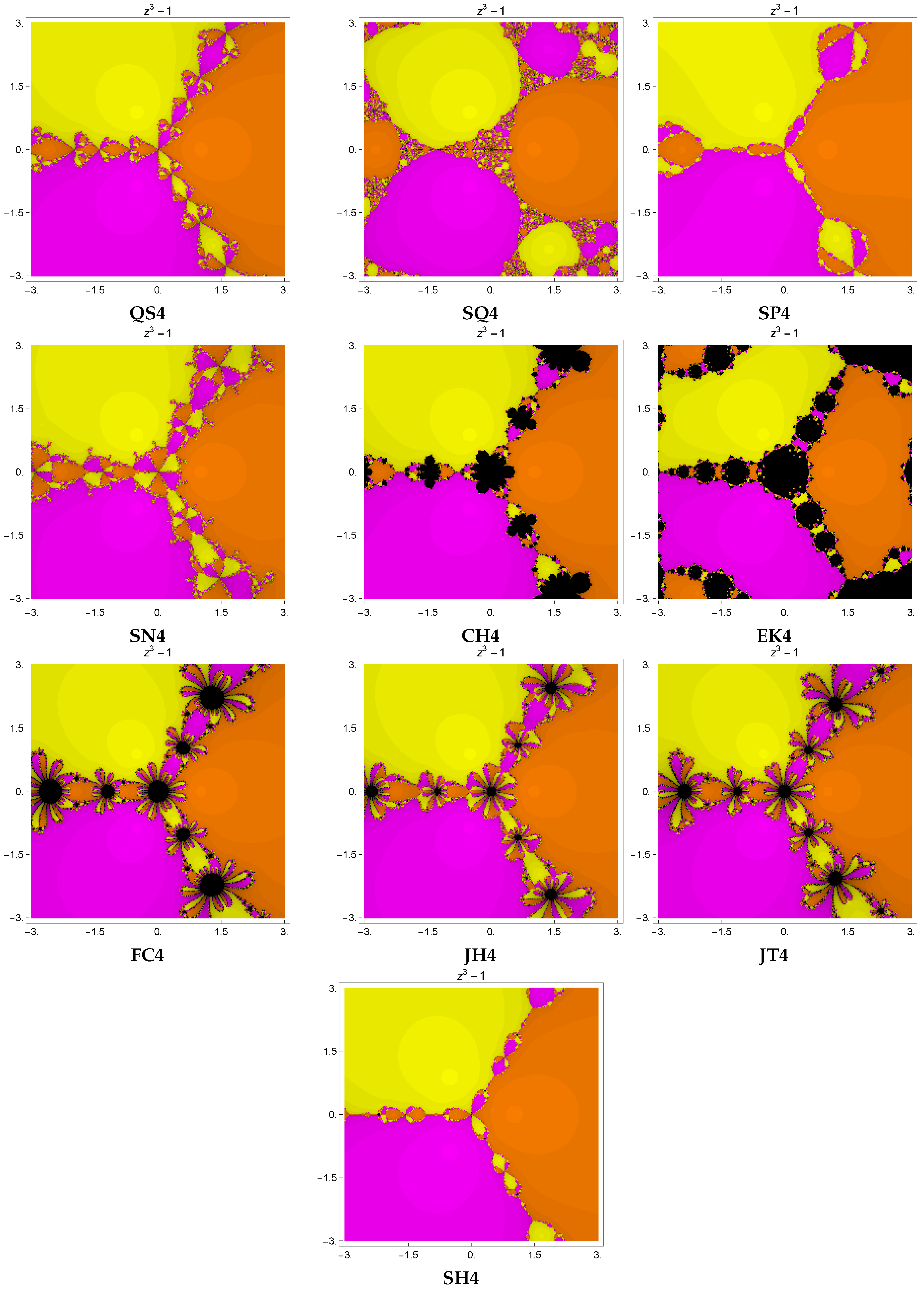
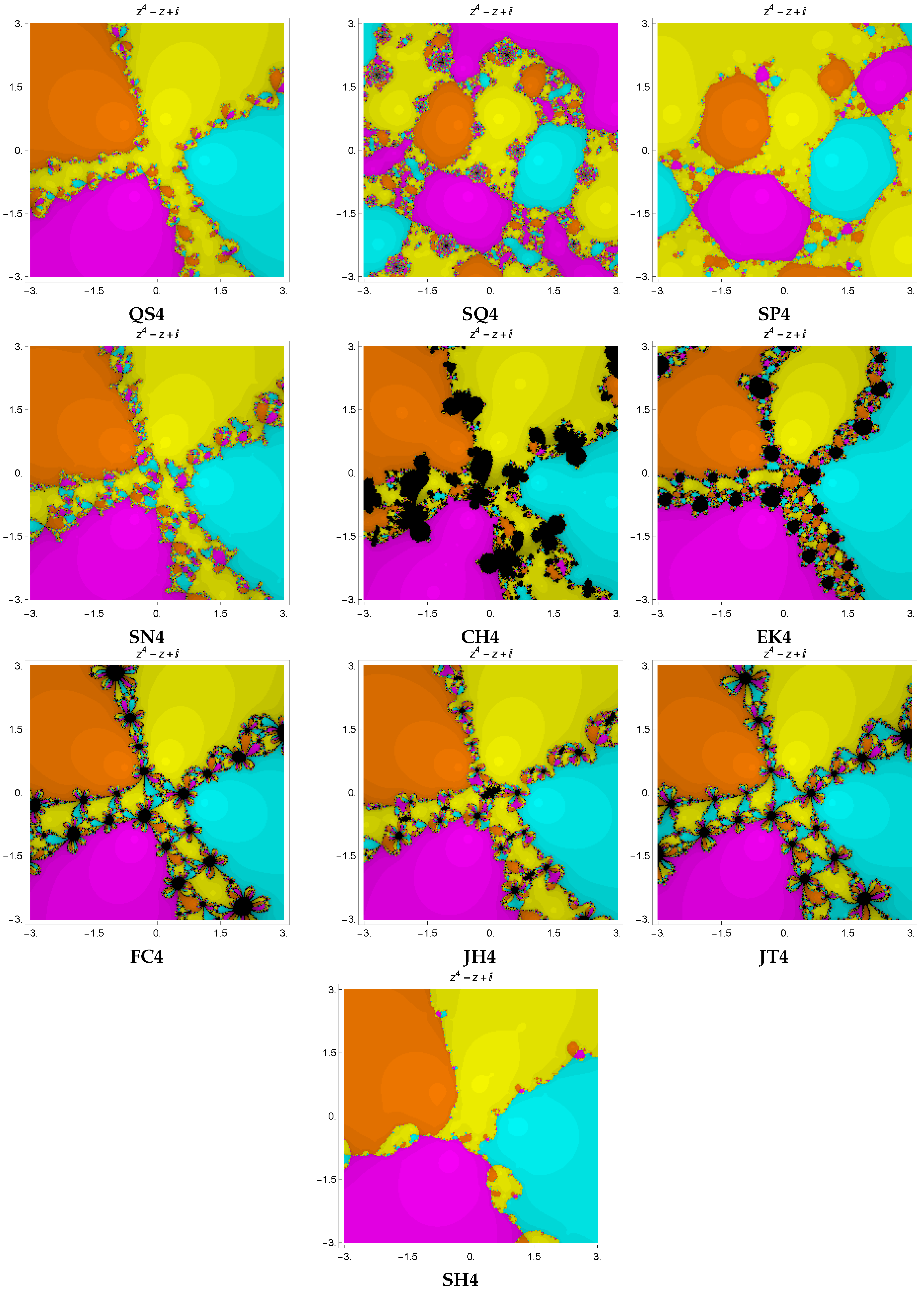
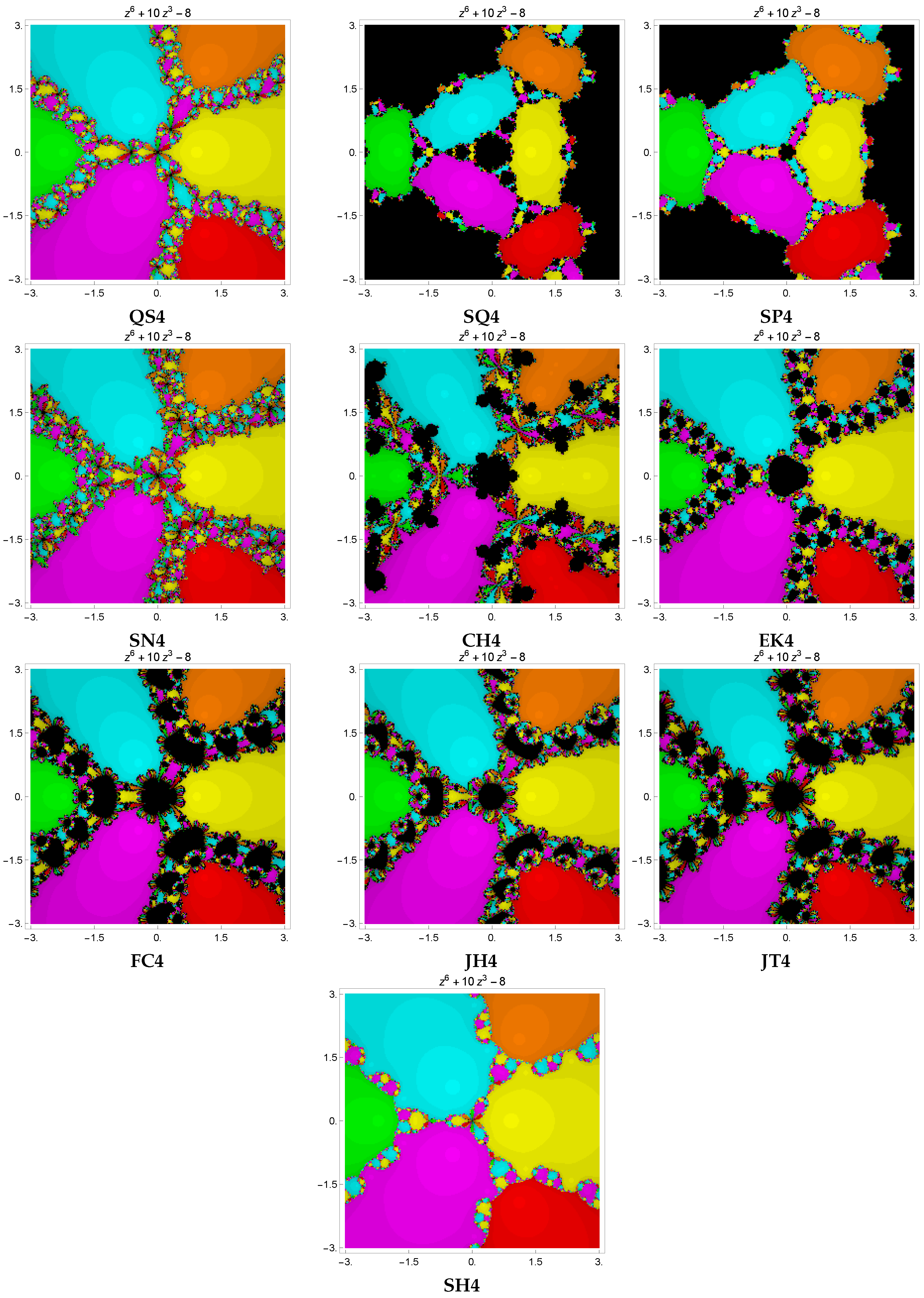
In order to plot the basins of attraction, we select a square region in the complex plane, labeled as I, that encompasses all of the roots of the complex polynomial under consideration. For a given initial point , distinct colors are allocated to different roots to which an iterative method converges. The presence of black-colored dots in the images indicates that the method did not succeed in finding a solution within the specified conditions, including the maximum number of iterations and the predetermined error threshold allowed to find the solution. The color brightness varies according to the number of iterations needed for convergence; a darker color indicates that more iterations are needed for the iterative technique to converge, while a brighter color specifies that fewer iterations are needed. We assume a maximum of 15 iterations and a tolerance of in this section. The number of black points in column number 3 shows that non-convergent points have a significant impact on the average number of iterations per point because they always require the maximum number of iterations allowed. Column 5 indicates the time it took to arrive at the solution, while column 4 displays the average number of iterations per point.
Example 1.


Consider the nonlinear function
having roots 1, and . The basins are depicted in Figure 1. The distinct methods , , and of the same order were compared with the new iterative approach . One can observe from Table 1 that our proposed method produces fewer black points as compared to others. Furthermore, a mean number of iterations is lower for than for the rest of the iterative techniques.

Figure 1.
Basins of attraction for optimal fourth-order iterative methods , , , , , , , , , generated for .

Table 1.
Comparison of optimal fourth-order Methods in terms of the number of black points, average number of iterations, and CPU time for .
Example 2.


Consider the nonlinear function:
The basins are depicted in Figure 2. The distinct methods , , , and of the same order were compared with the new iterative approach . One can observe from Table 2 that basins of attraction for the proposed method contain fewer black points as compared to others. Furthermore, the mean number of iterations is lower for than for the rest of the techniques.

Figure 2.
Basins of attraction for optimal fourth-order iterative methods , , , , , , , , , for .

Table 2.
Comparison of optimal fourth-order methods in terms of number of black points, average number of iterations and CPU time for .
Example 3.


Consider the nonlinear function:
having roots ,, , , and . The basins are depicted in Figure 3. The distinct methods , , and of the same order were compared with the new iterative approach . One can observe from Table 3 that basins of attraction for the proposed method contain fewer black points as compared to others. Furthermore, the mean number of iterations is less for than for the rest of the techniques.

Figure 3.
Basins of attraction for optimal fourth-order iterative methods , , , , , , , , , for .

Table 3.
Comparison of optimal fourth-order methods based on number of black points, average iterations, and CPU time for .
Example 4.
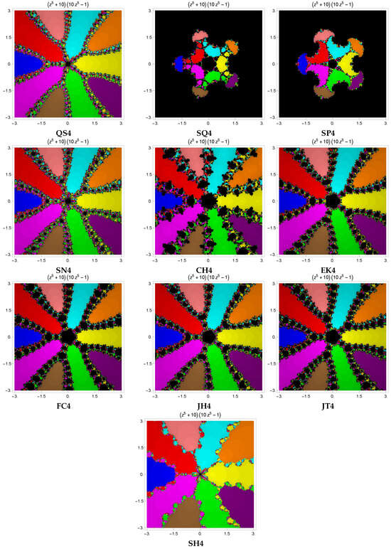

Consider the nonlinear function:
having roots
. The basins are depicted in Figure 4. The distinct methods , , and of the fourth order are compared with the new iterative approach . One can observe from Table 4 that the basins of attraction for the proposed method have fewer black points as compared to others. Furthermore, mean number of iterations is less for than for the rest of the techniques.

Figure 4.
Basins of attraction for optimal fourth-order iterative methods , , , , , , , , , for .

Table 4.
Comparison of optimal fourth-order methods based on number of black points, average iterations, and CPU time for .
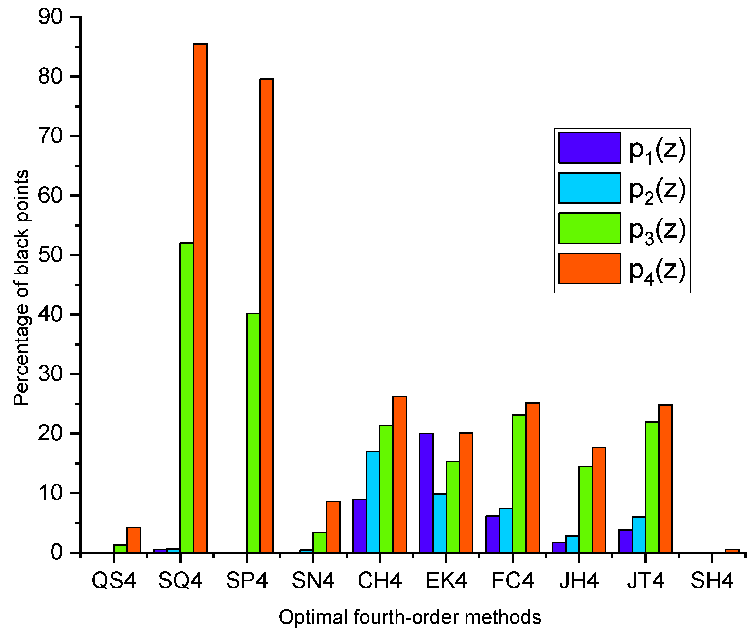
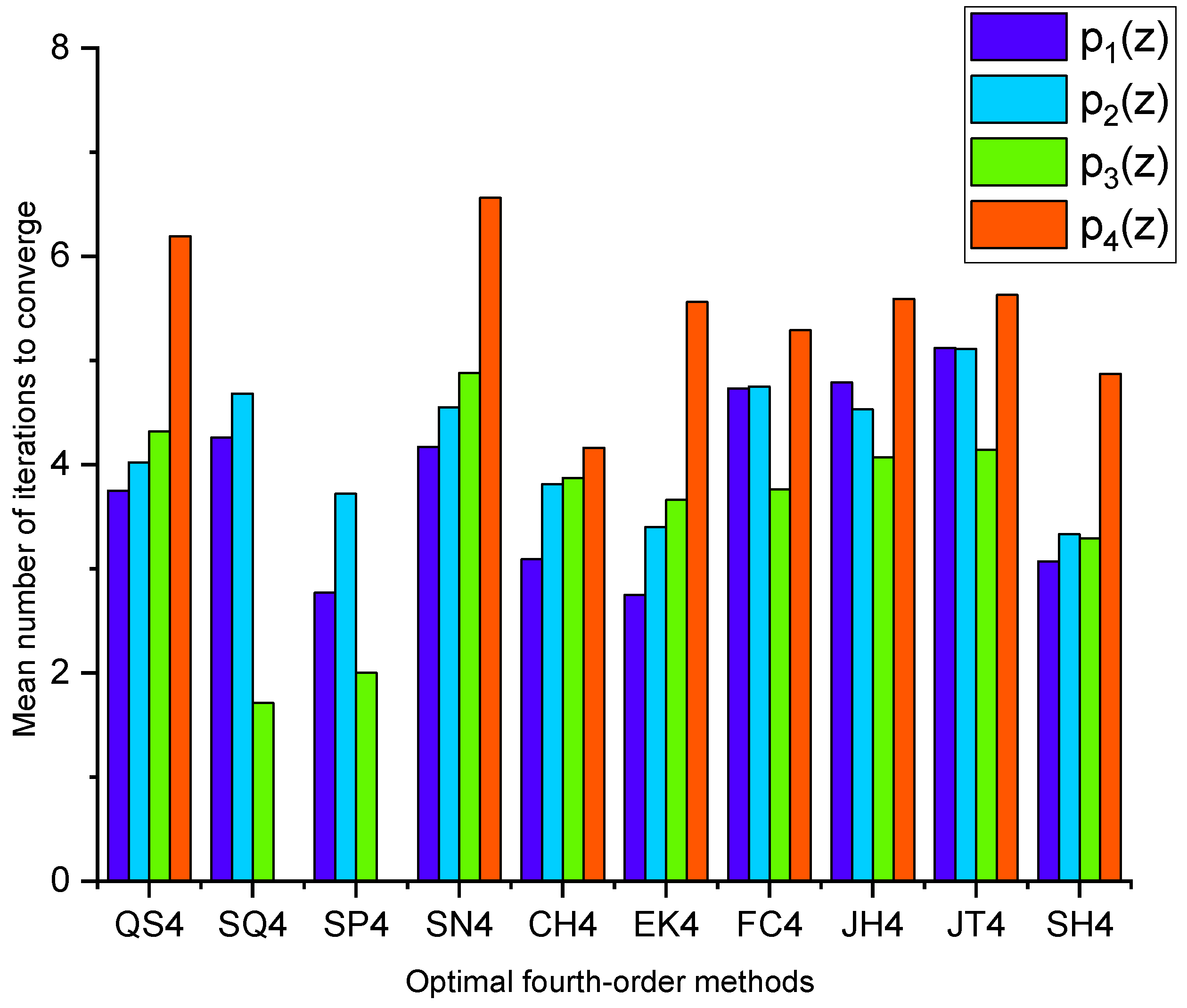
Moreover, Figure 5 and Figure 6 depict the graphical comparison among various iterative methods based on the number of black points and the mean number of iterations required for convergence, respectively.
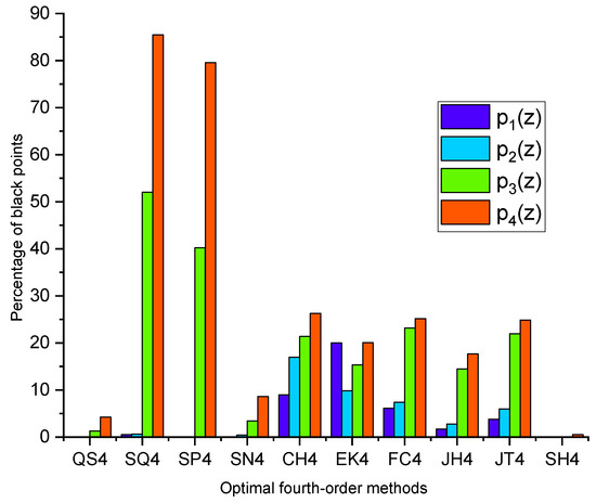
Figure 5.
Graphical comparison of optimal fourth-order methods based on the percentage of black points for , , and .
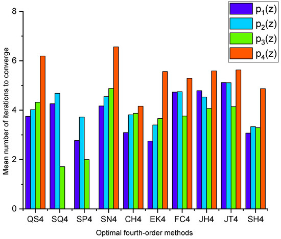
Figure 6.
Graphical comparison of optimal fourth-order methods based on the mean number of iterations to converge for , , and .
From Table 1, Table 2, Table 3 and Table 4 and Figure 1, Figure 2, Figure 3 and Figure 4, it is evident that our proposed method excels by demonstrating larger basins of attraction and fewer divergent points compared to other methods. Furthermore, it is observed from Table 3 and Table 4 and Figure 3 and Figure 4 that for Examples 3 and 4, most of the recently available optimal iterative algorithms failed to converge for solving highly complex problems since they provide a large number of black dots and a small area of convergence while the presented method remains effective in these circumstances.
5. Numerical Experiments
In this numerical study, we investigate numerical comparison of several iterative methods for solving some application-oriented nonlinear equations. To evaluate the performance of our recently developed iterative approach and to demonstrate its applications, some real-life application-based problems and their numerical solutions found by applying several iterative schemes are presented in this section.
The programming package was used for all numerical computations and the results were rounded to 2000 significant digits to obtain accurate results. Table 5, Table 6, Table 7, Table 8, Table 9 and Table 10 show the absolute residual error , the absolute error in the approximation of the root (() for the initial three iterations, the computational order of convergence and the CPU time in seconds, for the different methods. Additionally, the CPU time (measured in seconds) required by each method is computed to achieve the stopping criterion condition . The computational order of convergence (COC) is given by the formula [19]:
All of the comparison results are shown in Table 5, Table 6, Table 7, Table 8, Table 9 and Table 10.

Table 5.
Numerical comparisons of several optimal fourth-order iterative methods for .

Table 6.
Numerical comparisons of several optimal fourth-order iterative methods for .

Table 7.
Numerical comparisons of several optimal fourth-order iterative methods for .

Table 8.
Numerical comparisons of several optimal fourth-order iterative methods for .

Table 9.
Numerical comparisons of several optimal fourth-order iterative methods for .

Table 10.
Numerical comparisons of several optimal fourth-order iterative methods for .
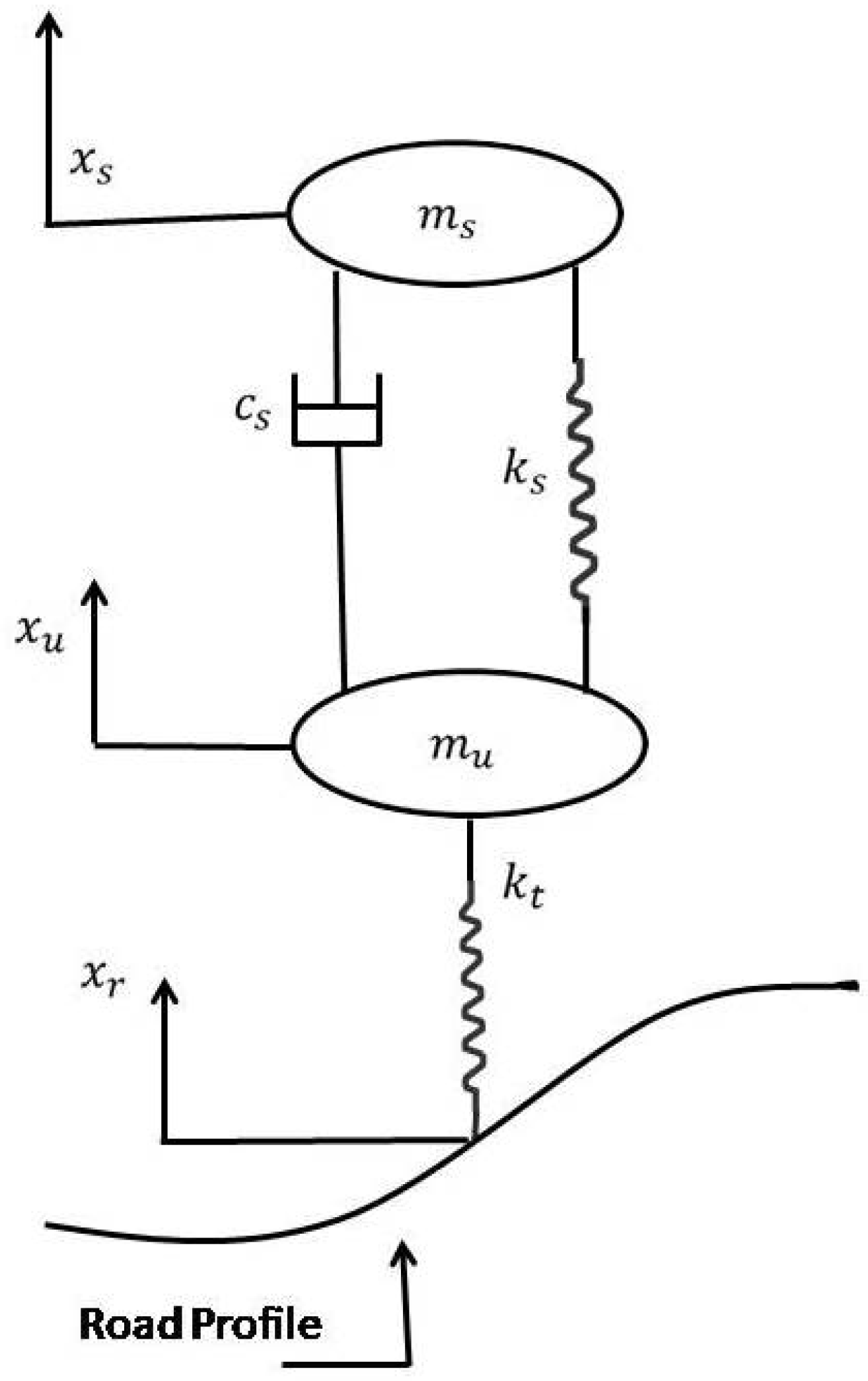
Problem 1: Quarter car suspension model [31]. The shock absorber (also called a damper) is an important component of the suspension system that controls the dynamic response of the vehicle’s mass as well as the mass of the suspension system (Konieczny [32] and Pulvirenti [33]). The shock absorber’s nonlinear properties make it one of the suspension system’s most intricate parts. An asymmetric nonlinear hysteresis loop [34] characterizes the damping force generated by the damper. The vehicle’s features are simulated in this study using a quarter-car model with two degrees of freedom. Comparing the effects of linear and nonlinear damping properties enables an investigation of the damper’s impact. Simple models, even linear and independently linear ones, are insufficient to adequately characterise the behavior of the damper. The mass motion equations are as follows [35]:
The spring stiffness and suspension coefficients in the tire stiffness system are represented by the symbols and , respectively. and stand for the masses above and below the springs, and and for their respective displacements. According to [31], the following polynomial is used to estimate the damping force coefficient F in Equation (30),
measuring the acceleration, velocity, and displacement of a mass over time (refer to Figure 7), where are exact roots of (31) up to ten decimal places.

Figure 7.
Quarter car suspension model.
Table 5 provides an in-depth comparison of various fourth-order optimal algorithms applied to the quarter car suspension model described in (31). Our proposed method, , demonstrates outstanding performance by achieving the smallest absolute error after the third iteration () and the lowest final function value (), indicating remarkable accuracy in the shortest time ( s), showcasing its efficiency in comparison with the other methods , , , and .
Problem 2: Hanging Object. The following nonlinear initial value problem originates from a situation in which a chain tied to an object on the ground is pushed upwards vertically by constant forces opposing gravity [36]:
By utilizing the method discussed in [37], a polynomial is employed to replicate Equation (32) as follows:
where denotes the exact solution of (33) up to four decimal places.
Table 6 provides the comparison of various fourth-order optimal algorithms applied to the hanging object problem given by (33). The proposed method, , shows better performance by achieving the smallest absolute error after the third iteration () and the lowest final function value () in the shortest time ( s), showcasing its efficiency.
Problem 3: Series circuit series analogue. Suppose we have a flexible spring with a mass m hanging from its free end, suspended vertically from a solid support. The mass attached to the spring controls how much it stretches or elongates; varied masses will result in different spring lengths. In accordance with Hooke’s law, a spring operates in the opposite direction of elongation and produces a restoring force, F, that is exactly proportional to the amount of elongation. In short, , where k denotes the spring constant, serves as the proportionality constant. The differential equation for an undamped spring mass system is symbolized by , which is mathematically represented as per [37]:
By utilizing the method discussed in [37], the polynomial is employed to replicate Equation (34) as follows:
denote the exact solution of (35) up to nine decimal places.
Table 7 provides a comparison of various fourth-order optimal algorithms applied to the series circuit analogue problem described in (35). The proposed method demonstrates outstanding performance in comparison with other methods, , , , and , by achieving the smallest absolute error after the third iteration () and the lowest final function value (), indicating remarkable accuracy. Moreover, provides these results in the shortest time ( s), showcasing its efficiency.
Problem 4: Civil Engineering Problem. You are designing a bookshelf with a height ranging from 8.5 inches to 11 inches and a total length of 29 inches. The shelf is made of wood with a Young’s Modulus of 3.66 Msi. It has a width of 12 inches and a thickness of 3/8 inches. Determine the maximum vertical deflection of the shelf in the figure:
The mathematical equation for the deflection of the shelf can be expressed as
In this example, u represents the position along the length of the beam. Therefore, to determine the optimal deflection, we need to find and perform the second derivative test, and thus,
The critical point for the deflection of the shelf, denoted as , occurs at a position of along the length of the beam. To determine the optimal deflection, we apply the second derivative test from single-variable calculus:
Now, at .
Hence, the minimum deflection of the shelf is at
Table 8 provides an in-depth comparison of various fourth-order optimal algorithms applied to the civil engineering problem described in (37). The performance of our proposed method, , is better than that of other methods like , , , and , as it produces the smallest absolute error after the third iteration () and the lowest final function value (), indicating remarkable accuracy in the shortest time ( s), showcasing its efficiency.
Problem 5: Chemical Engineering Problem [27]. The concentration of determines the acidity of a solution containing in :
The following nonlinear model is obtained by defining x as 104 times the hydronium ion concentration as
where are all the desired roots of Equation (40).
Table 9 provides the numerical comparison of various fourth-order optimal algorithms applied to the chemical engineering problem described in (40). Our proposed method, , demonstrates outstanding performance by achieving the smallest absolute error after the third iteration () and the lowest final function value (), indicating remarkable accuracy. Moreover, delivers these results in the shortest time ( s), showcasing its efficiency in comparison with , and .
Problem 6: Blood rheology model [38]. Blood rheology is the field of medical science that studies the physical and flow characteristics of blood. Blood’s non-Newtonian behavior often leads to its description as a Casson fluid. A simple fluid, such as blood or water, flows through a tube in a way that produces a velocity gradient along the tube walls. This fluid moves as a cohesive plug with little deformation, in accordance with the flow characteristics of a Casson fluid. Upon investigating the plug flow of Caisson fluid, particular attention is directed towards the following nonlinear equation:
where u denotes the plug flow of Caisson fluid flow. One root of the Equation (41) is
Table 10 provides an in-depth comparison of various fourth-order optimal algorithms applied to the blood rheology model described in (41). The proposed method, , demonstrates efficient performance by achieving the smallest absolute error after the third iteration (), () and the lowest final function value (), (), respectively, indicating remarkable accuracy. Moreover, delivers these results in the shortest time ( s), showcasing its efficiency in comparison with other methods, , , and .
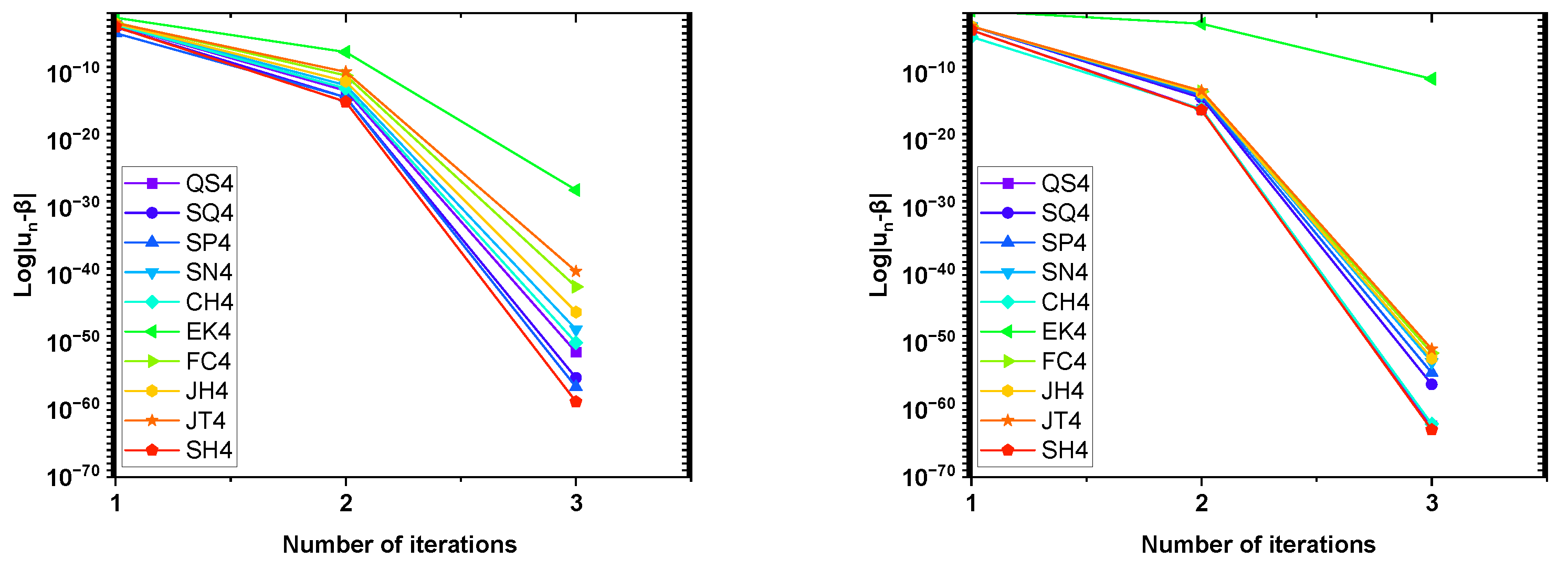
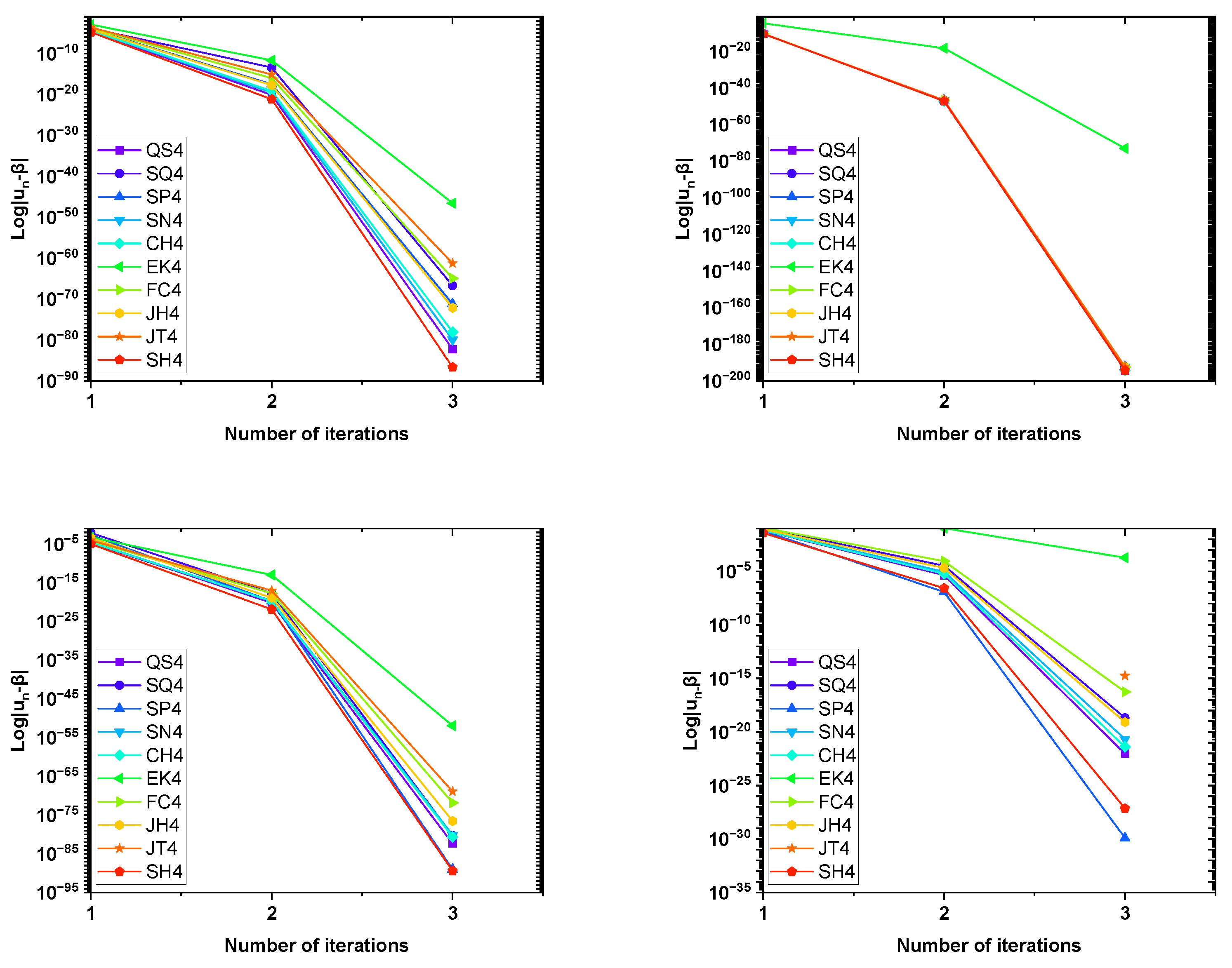
Furthermore, Figure 5, Figure 6 and Figure 8 illustrate the graphical comparison of the different fourth-order optimal methods based on a percentage of black points, the mean number of iterations for methods to converge, and the absolute error in consecutive iterations represented as after completing three iterations, respectively. The Figure 5, Figure 6 and Figure 8 show that the proposed method is highly competitive, demonstrating fast convergence towards the root in less CPU time and possesses superior accuracy compared to other well-known methods.
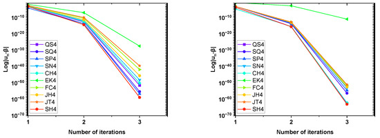
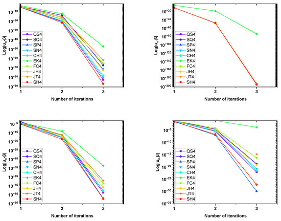
Figure 8.
Comparison of the optimal fourth-order methods based on the absolute error, , after the first three full iterations for , , , , and respectively.
6. Conclusions
We employed the weight function technique to devise a two-step fourth-order optimal iterative method aimed at solving nonlinear equations. We present a thorough convergence investigation and employed basins of attraction to evaluate the stability of the techniques. Our proposed algorithm performs better in terms of the errors in the consecutive iterations, residual errors and CPU time calculated in seconds. Additionally, the proposed method exhibits the lowest percentage of black points and requires the fewest average number of iterations to converge to the required solution. Analysis of basins of attraction in the complex plane, along with numerical results in the real domain, demonstrate that the newly devised method showcases superior stability and accuracy compared to other methods of the same order.
Author Contributions
Conceptualization, S.A. and N.C.; Methodology, S.A. and N.C.; Validation, S.D., M.-u.-D.J. and N.C.; Formal Analysis, M.-u.-D.J. and T.A.; Investigation, S.D. and M.-u.-D.J.; Writing−Original Draft Preparation, S.A., N.C. and M.-u.-D.J.; Writing−Review & Editing, S.D., M.-u.-D.J. and T.A.; Visualization, S.A. and M.-u.-D.J.; Supervision, N.C. and S.D. All authors have read and agreed to the published version of the manuscript.
Funding
This research received no external funding.
Data Availability Statement
Enquiries about data availability should be directed to the authors.
Conflicts of Interest
There are no conflicts of interest among all the authors.
References
- Tsoulos, I.; Stavrakoudis, A. On locating all roots of systems of nonlinear equations inside bounded domain using global optimization methods. Nonlinear Anal. Real World Appl. 2010, 11, 2465–2471. [Google Scholar] [CrossRef]
- Awawdeh, F. On new iterative method for solving systems of nonlinear equations. Numer. Algorithms 2010, 54, 395–409. [Google Scholar] [CrossRef]
- Lin, Y.; Bao, L.; Jia, X. Convergence analysis of a variant of the Newton method for solving nonlinear equations. Comput. Math. Appl. 2010, 59, 2121–2127. [Google Scholar] [CrossRef]
- Grosan, C.; Abraham, A. A new approach for solving nonlinear equations systems. IEEE Trans. Syst. Man Cybern.-Part A Syst. Humans 2008, 38, 698–714. [Google Scholar] [CrossRef]
- Kaplan, E.D.; Hegarty, C. Understanding GPS/GNSS: Principles and Applications; Artech House: London, UK, 2017. [Google Scholar]
- Rouzbar, R.; Eyi, S. Reacting flow analysis of a cavity-based scramjet combustor using a Jacobian-free Newton–Krylov method. Aeronaut. J. 2018, 122, 1884–1915. [Google Scholar] [CrossRef]
- Nourgaliev, R.; Greene, P.; Weston, B.; Barney, R.; Anderson, A.; Khairallah, S.; Delplanque, J.P. High-order fully implicit solver for all-speed fluid dynamics: AUSM ride from nearly incompressible variable-density flows to shock dynamics. Shock Waves 2019, 29, 651–689. [Google Scholar] [CrossRef]
- Zhang, H.; Guo, J.; Lu, J.; Niu, J.; Li, F.; Xu, Y. The comparison between nonlinear and linear preconditioning JFNK method for transient neutronics/thermal-hydraulics coupling problem. Ann. Nucl. Energy 2019, 132, 357–368. [Google Scholar] [CrossRef]
- Ortega, J.M. Numerical Analysis: A Second Course; SIAM: Philadelphia, PA, USA, 1990. [Google Scholar]
- Kung, H.; Traub, J.F. Optimal order of one-point and multipoint iteration. J. ACM 1974, 21, 643–651. [Google Scholar] [CrossRef]
- Kou, J.; Li, Y.; Wang, X. A composite fourth-order iterative method for solving non-linear equations. Appl. Math. Comput. 2007, 184, 471–475. [Google Scholar] [CrossRef]
- Sharma, H.; Kansal, M.; Behl, R. An Efficient Optimal Derivative-Free Fourth-Order Method and Its Memory Variant for Non-Linear Models and Their Dynamics. Math. Comput. Appl. 2023, 28, 48. [Google Scholar] [CrossRef]
- Nadeem, A.; Ali, F.; He, J.H. New optimal fourth-order iterative method based on linear combination technique. Hacet. J. Math. Stat. 2021, 50, 1692–1708. [Google Scholar] [CrossRef]
- Panday, S.; Sharma, A.; Thangkhenpau, G. Optimal fourth and eighth-order iterative methods for non-linear equations. J. Appl. Math. Comput. 2023, 69, 953–971. [Google Scholar] [CrossRef]
- Kansal, M.; Cordero, A.; Bhalla, S.; Torregrosa, J.R. New fourth-and sixth-order classes of iterative methods for solving systems of nonlinear equations and their stability analysis. Numer. Algorithms 2021, 87, 1017–1060. [Google Scholar] [CrossRef]
- Qureshi, S.; Argyros, I.K.; Soomro, A.; Gdawiec, K.; Shaikh, A.A.; Hincal, E. A new optimal root-finding iterative algorithm: Local and semilocal analysis with polynomiography. Numer. Algorithms 2024, 95, 1715–1745. [Google Scholar] [CrossRef]
- Jaiswal, J.; Choubey, N. A new efficient optimal eighth-order iterative method for solving nonlinear equations. arXiv 2013, arXiv:1304.4702. [Google Scholar]
- Choubey, N.; Jaiswal, J.P. An improved optimal eighth-order iterative scheme with its dynamical behaviour. Int. J. Comput. Sci. Math. 2016, 7, 361–370. [Google Scholar] [CrossRef]
- Petković, M.S.; Neta, B.; Petković, L.D.; Džunić, J. Multipoint methods for solving nonlinear equations: A survey. Appl. Math. Comput. 2014, 226, 635–660. [Google Scholar] [CrossRef]
- King, R.F. A family of fourth order methods for nonlinear equations. SIAM J. Numer. Anal. 1973, 10, 876–879. [Google Scholar] [CrossRef]
- Sharma, J. A composite third order Newton–Steffensen method for solving nonlinear equations. Appl. Math. Comput. 2005, 169, 242–246. [Google Scholar] [CrossRef]
- Potra, F.A.; Pták, V. Nondiscrete Induction and Iterative Processes; Research Notes in Mathematics; Pitman Advanced Pub.: Boston, MA, USA, 1984; Volume 103. [Google Scholar]
- Chun, C.; Lee, M.Y.; Neta, B.; Džunić, J. On optimal fourth-order iterative methods free from second derivative and their dynamics. Appl. Math. Comput. 2012, 218, 6427–6438. [Google Scholar] [CrossRef]
- Junjua, M.u.D.; Akram, S.; Yasmin, N.; Zafar, F. A New Jarratt-Type Fourth-Order Method for Solving System of Nonlinear Equations and Applications. J. Appl. Math. 2015, 2015, 805278. [Google Scholar] [CrossRef]
- Chicharro, F.I.; Cordero, A.; Garrido, N.; Torregrosa, J.R. Wide stability in a new family of optimal fourth-order iterative methods. Comput. Math. Methods 2019, 1, e1023. [Google Scholar] [CrossRef]
- Sharma, E.; Panday, S.; Dwivedi, M. New optimal fourth order iterative method for solving nonlinear equations. Int. J. Emerg. Technol. 2020, 11, 755–758. [Google Scholar]
- Abdullah, S.; Choubey, N.; Dara, S. Optimal fourth-and eighth-order iterative methods for solving nonlinear equations with basins of attraction. J. Appl. Math. Comput. 2024, 70, 3477–3507. [Google Scholar] [CrossRef]
- Qureshi, S.; Chicharro, F.I.; Argyros, I.K.; Soomro, A.; Alahmadi, J.; Hincal, E. A New Optimal Numerical Root-Solver for Solving Systems of Nonlinear Equations Using Local, Semi-Local, and Stability Analysis. Axioms 2024, 13, 341. [Google Scholar] [CrossRef]
- Singh, A.; Jaiswal, J. Several new third-order and fourth-order iterative methods for solving nonlinear equations. Int. J. Eng. Math 2014, 2014, 828409. [Google Scholar] [CrossRef]
- Stewart, B.D. Attractor Basins of Various Root-Finding Methods. Ph.D. Thesis, Naval Postgraduate School, Monterey, CA, USA, 2001. [Google Scholar]
- Barethiye, V.; Pohit, G.; Mitra, A. Analysis of a quarter car suspension system based on nonlinear shock absorber damping models. Int. J. Automot. Mech. Eng. 2017, 14, 4401–4418. [Google Scholar] [CrossRef]
- Konieczny, Ł. Analysis of simplifications applied in vibration damping modelling for a passive car shock absorber. Shock Vib. 2016, 2016, 6182847. [Google Scholar] [CrossRef]
- Pulvirenti, G.; Faria, C. Influence of Housing Wall Compliance on Shock Absorbers in the Context of Vehicle Dynamics. Proc. IOP Conf. Ser. Mater. Sci. Eng. 2017, 252, 012026. [Google Scholar] [CrossRef]
- Liu, Y.; Zhang, J. Nonlinear dynamic responses of twin-tube hydraulic shock absorber. Mech. Res. Commun. 2002, 29, 359–365. [Google Scholar] [CrossRef]
- Shams, M.; Carpentieri, B. Efficient Inverse Fractional Neural Network-Based Simultaneous Schemes for Nonlinear Engineering Applications. Fractal Fract. 2023, 7, 849. [Google Scholar] [CrossRef]
- Shams, M.; Carpentieri, B. On highly efficient fractional numerical method for solving nonlinear engineering models. Mathematics 2023, 11, 4914. [Google Scholar] [CrossRef]
- Shams, M.; Kausar, N.; Yaqoob, N.; Arif, N.; Addis, G.M. Techniques for finding analytical solution of generalized fuzzy differential equations with applications. Complexity 2023, 2023, 3000653. [Google Scholar] [CrossRef]
- Qureshi, S.; Soomro, A.; Shaikh, A.A.; Hincal, E.; Gokbulut, N. A Novel Multistep Iterative Technique for Models in Medical Sciences with Complex Dynamics. Comput. Math. Methods Med. 2022, 2022, 7656451. [Google Scholar] [CrossRef] [PubMed]
Disclaimer/Publisher’s Note: The statements, opinions and data contained in all publications are solely those of the individual author(s) and contributor(s) and not of MDPI and/or the editor(s). MDPI and/or the editor(s) disclaim responsibility for any injury to people or property resulting from any ideas, methods, instructions or products referred to in the content. |
© 2024 by the authors. Licensee MDPI, Basel, Switzerland. This article is an open access article distributed under the terms and conditions of the Creative Commons Attribution (CC BY) license (https://creativecommons.org/licenses/by/4.0/).

