


Abstract
Larceny is considered a high-impact crime in Mexico City because of its effect on public perceptions of safety. Understanding its spatial and temporal dynamics is therefore important for designing effective public safety policies. This study extends the Trajectory Analysis framework to examine the spatio-temporal evolution of larceny in Mexico City from 2020 to 2024. The proposed approach incorporates Kendall’s Tau () to quantify trend strength across trajectory types, including Gain, Loss, and alternation patterns, and introduces a multi-resolution analysis to identify and quantify spatial exchange patterns in crime distribution. Results indicate an overall decline in larceny across the city, but also reveal spatial exchanges, suggesting that reductions in some areas may reflect displacement rather than elimination. By capturing both crime reduction and redistribution patterns, the framework provides a more nuanced basis for data-driven public safety strategies.
1. Introduction
Assessing public safety is a challenging responsibility for governments, since it is threatened by diverse criminal activities. In Mexico, crimes are classified into two categories: federal jurisdiction and common law.
On the one hand, crimes of federal jurisdiction affect the country’s interests and are beyond the action limits of a state or municipality. Drug trafficking, organized crime, electoral crimes, tax crimes, crimes against health, among others, are in this category. On the other, common law ones affect individuals in a state or municipality. This category includes for example, injury crimes against family and larceny for which the municipal authorities are competent to analyze, react, and implement strategies to control this social phenomenon. One main difference is that street crime is handled by local governments and they also have different legislation (each state has its own penal code and there is a single federal penal code, accompanied by special federal laws). In both cases, graphical tools for effective description and communication are required.
Statistical graphical tools are useful to describe and communicate complex scenarios in simple terms to help policymakers design public policies and campaigns to meet goals, such as reducing the incidence of specific types of crime. In this regard, visualization tools for describing, communicating, and evaluating both the criminal situation and effectiveness of public policies are scarce [1,2].
Aligned with the need for statistical graphical tools, we present an application of the count-based Trajectory Analysis Framework proposed by Bilintoh et al. [3], referred to as the framework. The framework provides a way to describe and discover spatio-temporal trend and evolution of binary events. We use this implementation to describe the spatio-temporal evolution of the larceny in Mexico City between 2020 and 2024.
In the count-based Trajectory Analysis framework, every cell is classified into one of eight categories, depending on its trajectories through the entire time interval in: (1) gain, (2) loss, (3) gain with alternation, (4) loss with alternation, (5) alternation with gain first, (6) alternation with loss first, (7) stable absence, and (8) stable presence. These eight categories allow for a precise and unambiguous description of the trajectory of pixels for three time intervals of binary changes, since the number of unique combinations is limited by the number of states raised to the power of the number of intervals .
These categories depend on the comparison of individual initial and final values of each pixel, discarding some of the dynamic details that occur during the time interval. For example, if a pixel has a presence value at the start of the time interval and an absence value at the end of its trajectory, then it is classified as a loss or loss with alternation, regardless of possible intermediate changes that may occur throughout the time interval. In this sense, larceny analysis incidence is temporally sensitive, and the trajectory classification may not be aligned with the general trend. For example, different interpretations may occur when a trajectory is classified as loss with alternation when it presents an increasing trend.
When the spatio-temporal time series is longer, these eight categories become insufficient to provide a good explanation of the observed dynamics. Accordingly, we propose the incorporation of the Kendall’s correlation coefficient which describes the strength of monotonic trajectory trends of time series. This helps complement the number of presence and number of changes maps produced by the presencePlot function in the timeseriesTrajectories R package (version 1.1.3) presented in [3]. Kendall’s is suitable and straightforward to implement in binary or rational numbers, is robust to outliers, and useful for assessing the temporal sensitivity of larceny occurrences during the entire time interval. This means that it considers the possibility of having a neutral or negative ordinal association between consecutive measurements even if there are losses or gains observed by chance in the time interval.
Our proposal also includes a method to quantify the exchange component at specific resolutions, which measures simultaneous displacements that produce gains and losses occurring among territorial sub-regions without affecting the net change of a variable during the time interval. In the context of criminal studies, the regional displacements in criminal events are referred to in the literature as spillover. The sub-region size where most spillover occurs is identified by quantifying the Exchange component across different resolutions and selecting the resolution with the smaller Exchange gain.
This application in criminality analysis adds to the list of spatio-temporal phenomena. It complements existing applications that study phenomena such as marsh evolution [4], soybean cultivation [5], wildfire dynamics [6], and avocado orchards [7], demonstrating its flexibility and relevance for the study of spatio-temporal phenomena in diverse contexts.
The rest of this manuscript is organized as follows. We first present work related to trajectory analysis and its connection with the study of larceny. Then, we introduce the basics of trajectory analysis framework of spatio-temporal data along with the study region and data used. This is followed by our contribution to the analysis, including the resolution analysis for the exchange component and the implementation of Kendall’s maps that enrich the trajectory analysis and the findings for larceny analysis. Lastly, we conclude with a discussion highlighting the strengths, areas of improvement and proposed future work.
2. Related Work
Trajectory analysis, a type of longitudinal analysis [8], is a sub-discipline of time series that studies graphical methods for descriptive and effective exploratory data analysis of spatio-temporal patterns and their relationship with other variables that influence their behavior.
In the social sciences, sequence analysis has been translated into a set of longitudinal data methods that study the outcomes [9]. Surveys tend to focus on highlighting the application of qualitative methods that study the population and their changes throughout time, also referred to as life course trajectories or event history trajectories [10]. Over time, computational approaches have been emphasized to characterize complex successions of different states [11], finding that social organization derives from spatial, hierarchical, and other ordered phenomena.
In criminology, trajectory analysis provides information that analysts can interpret and articulate to propose hypotheses that guide the confection of strategies to control crime incidence. It has also been used to examine how large samples of individuals could be grouped according to crimes throughout life [12]. More recently, longitudinal analyses have been applied at the place scale to identify trends and clusters of street segments in terms of crime incidences [13] and micro-geographic hotspots [14].
Some spatio-temporal methods require the use of individual incidents and rely on global tests such as the Knox index, which is based on a Chi-square test of independence between expected and observed counts given time and space thresholds. On that same scale, the near-repeat method is a more recent version of the Knox index used to identify spatio-temporal interactions [15,16,17]. Other techniques oriented toward the prediction and projection of rates or counts include conditional autoregressive models, which are widely used in spatial epidemiology [18]. With the development of machine learning models, the risk terrain modeling method has been proposed, which also serves the purpose of making predictions [19].
Cluster analysis methods have also been adapted to extend to spatio-temporal patterns. They result in the characterization of trajectories in other longitudinal studies of crime [20,21]. This last example implements the classification of trajectories with a longitudinal k-means algorithm. It identifies groups of spatial units with similar behaviors suggesting to retain the information of time and place of each event and calculate its frequency by using count-based methods.
Local spatio-temporal techniques are less developed, like the use of spatio-temporal k-means adaptations, but it is not a widely used technique. Arguably, the emerging hotspot analysis constitutes the closest technique to trajectory analysis, particularly in our proposal. It is based on the combination of the Getis-Ord statistic to identify two classes of positive spatial autocorrelation—strong and weak—also known as hot and cold spots. The results are then combined with Kendall’s Tau to classify the spatial results of each unit along the temporal analysis vector into up to 36 classes. In contrast, our trajectory-based proposal yields more directly interpretable sequences of movement in space–time.
Examples of the application of the count-based trajectory analysis include measuring and tracking the trajectories of losses and gains of soybean cultivation [5] and to cross-compare marsh evolution in three sites within the United States Long-Term Ecological Research Network [4]. Both use the proposed count-based framework for a time series trajectory analysis to describe spatio-temporal changes in land cover to elucidate details and differences of the evolution of certain types of cover. In these last contributions, a highlight is the possibility to use different temporal resolutions in the study, while keeping the spatial resolution fixed.
In the context of this work, ‘count-based’ means we do not use a binary variable representing presence or absence, but rather a non-negative integer assigned to each cell at a specific resolution representing the aggregated count of the incidents. We opt to use that term to distinguish the framework from others found in the literature.
The methodology proposed in [4] is a recent approach and, thus, the diversity of applications is yet scarce. In this sense we propose the use of this methodology for a spatio-temporal graphical analysis of the dynamics of larceny theft. But first, we briefly explain this methodology in the next section.
3. Materials and Methods
3.1. Study Area and Data
The region of study is the capital of Mexico, Mexico City. It is located in the south-central region of the country, and covers an approximate area of 1495 km2. This region represents the smallest state with roughly 0.1% of the whole country [22]. In addition, it is subdivided into 16 municipalities. Despite its size, Mexico City is one of the most densely populated regions in the world with 9.2 million people, representing 7.3% of the Mexican population in the country. This results in a population density of approximately 8400 inhabitants per km2, placing it above Tokyo, Japan (~6500 people/km2) and below Seoul, South Korea (~10,000 people/km2) [23].
In 2024, the National Institute of Statistics and Geography carried out the 14th installment of the National Survey of Victimization and Perception of Public Safety [24]. According to its results, roughly one third of households in the city reported being victims of crime incidence. This contrasts with official reports of decreasing trends between 2020 and 2024.
In this context, the spatio-temporal complexity of the phenomenon makes it difficult to gain a clear understanding of the evolution of this type of crime. Therefore it is pertinent to identify and describe relevant spatio-temporal patterns of this reported decrease, so that it is easy to identify criminal displacement of hot spots. Not all crime types behave the same way, and some are more under-reported than others.
According to the Human Development Report for Latin America 2013–2014 of the United Nations Development Programme [25], street crime is among the six main threats to citizen security. This type of crime refers to theft and robbery on a small scale that tend to occur in public places and that involve, in some cases, threats of violence, beatings, or injuries inflicted on victims. To contextualize the situation of victimization in Mexico, the National Survey of Victimization and Perception of Public Security [24] reports that street crime occurs more frequently than other crimes. At the national level, it reaches 34.8%, while in Mexico City it is 51% from 2014 to 2023. While street robbery generally involves the loss of valuables or small belongings, its high frequency significantly impacts the public’s perception of insecurity. This perception often manifests as fear of crime, understood as the emotional reaction—such as fear or anxiety—to the possibility of being a crime victim. Specifically, in the case of larceny, this fear increases because people perceive that they cannot control their surroundings while walking on the street or waiting for transportation [26]. Thus, the prevalence of street theft underscores how fear of crime can transform perceptions of insecurity, making theft a high-impact crime for local authorities. We thus pay attention to larceny crimes which serve as a proxy to the sense of insecurity by the population.
Larceny incidence data in Mexico City is reported by the Office of the Attorney General of Mexico City [27] and made publicly available roughly every six months. For this study, we consider data from years 2020 to 2024 containing just over 47,500 georeferenced data points distributed in the city.
Mexico City’s Secretariat of Citizen Security organizes the city into 71 territorial units, called jurisdictions, for policing and monitoring purposes. These jurisdictions have diverse shapes and areas ranging from 1.08 to 73.43 km2. The area distribution of the jurisdictions is as follows: 38 jurisdictions have an area between 1.08 and 10 km2, 25 between 10 and 20 km2 and 8 between 20 and 73.43 km2. This diversity complicates a straightforward analysis and comparison of larceny incidence trajectories with respect to population at risk among jurisdictions and also the definition of priority areas.
This motivates the territorial re-organization in regular square tessellation cells at resolutions of 100, 200, 400, 800, 1600, and 3200 m. The total number of cells that cover Mexico City at the different resolutions are listed in Table 1.
Table 1.
Resolution and number of cells needed to cover Mexico City.
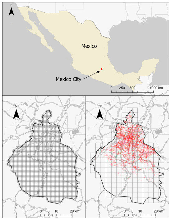
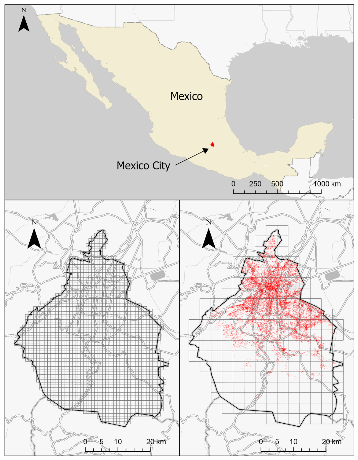
Figure 1 shows the administrative boundary of Mexico City, its coverage with regular square tessellation cells at 100 and 3200 m of resolution, and the georeferenced larceny events represented by the red data points reported from 2020 to 2024.
Figure 1.
Area of study and data: The location of Mexico City, its administrative boundary, the 100 and 3200 m resolution cells that cover it, and all data points. Country and city boundaries were obtained from the National Institute of Statistics and Geography’s (INEGI) National Geostatistical Framework. The country boundary is in WGS84 (EPSG:4326) and the city’s in UTM Zone 14N (EPSG:32614).
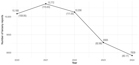
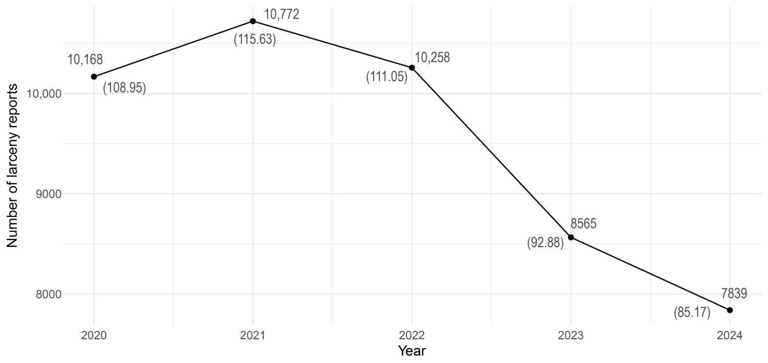
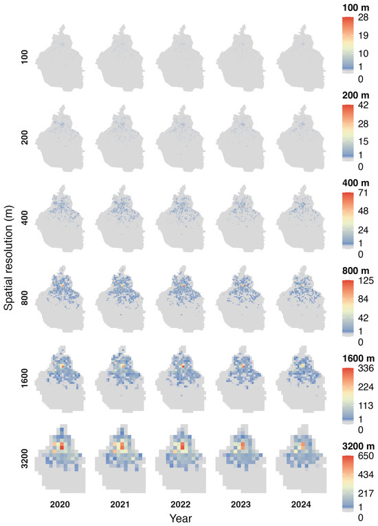
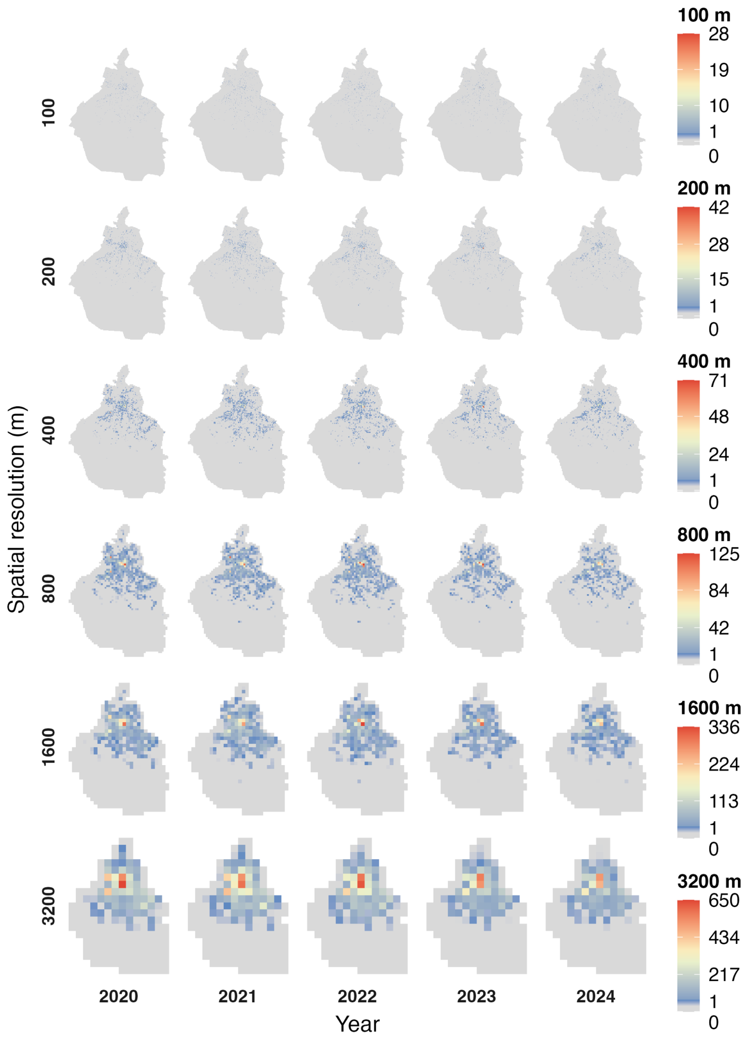
Figure 2 shows the number of larceny reports per year and Figure 3 shows the counts of larceny events as the sum at all time points and resolutions.
Figure 2.
Temporal evolution of georeferenced larceny reports from 2020 to 2024. Number of reports are shown together with per capita rates in parenthesis.
Figure 3.
Counts of larceny events per cell for different years and resolutions from 2020 to 2024.
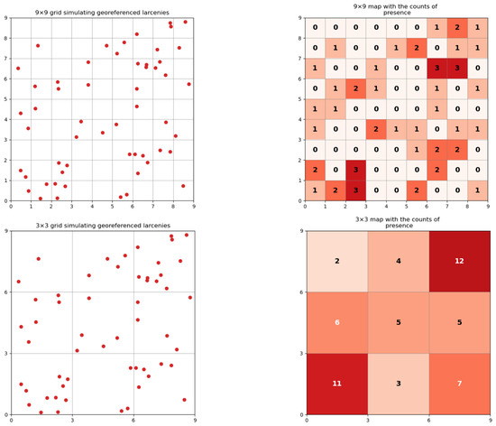
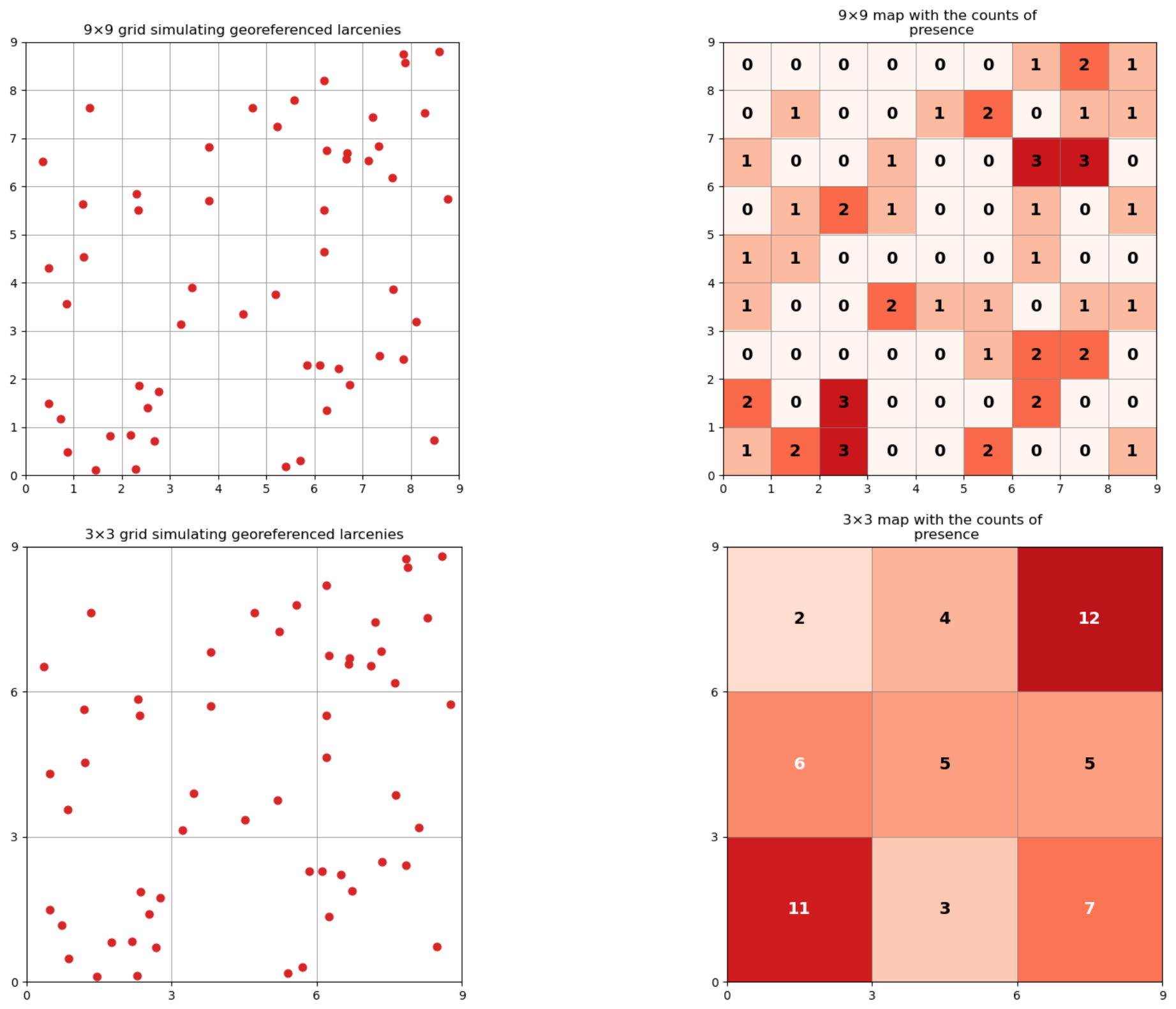
An example of how raster maps are generated from the georeferenced data is shown in Figure 4. The first row represents a raster aggregating georeferenced larcenies within cells at 1 unit of resolution and the second one represents the same georeferenced larcenies at units of twice the resolution. This is a sample of the format used as inputs for the trajectory analysis.
Figure 4.
Example of a raster map generation from raw georeferenced data.
3.2. Trajectory Analysis
The framework [3] comprises a set of arithmetic and graphical tools to quantify, describe, and identify spatio-temporal patterns of a binary or rational positive spatial variable from time-series of maps . Each map is a georeferenced map projected in an array of cells with an identifier m, where M denotes the number of cells. The framework relies on classifying trajectories in eight categories and the spatio-temporal description of gains or losses sequence. In this regard, the framework uses graphical tools like stack bar plots, which describe the spatio-temporal components like exchange, alternation, and net change. We aim to extending this framework by taking into account time-sensitive variations using Kendall’s coefficient for each trajectory, which is explained in more detail in Section 3.2.2.
As an example, consider the information from a binary time series of four maps where each trajectory’s index is shown in column m in Table 2. This time series of maps produces three maps of gains and losses. The column shows this coefficient for each trajectory, and the Trajectory Classification column indicates the class of the trajectory as one of the eight possible classes: (1) Stable Absence, (2) Stable Presence, (3) Loss without alternation, (4) Gain without alternation, (5) All alternation Gain first, (6) All alternation Loss First, (7) Loss with Alternation, and (8) Gain with alternation.
Table 2.
Trajectory classes for the case of four maps generating three time intervals. Hollow squares represent absence and solid ones, presence.
The classification rule for each trajectory is as follows: if trajectories experiment no change, they are classified as Stable Presence or Stable Absence. Trajectories 1 and 2 satisfy this criterion. If a trajectory only shows one change, then it can be classified as either Loss Without Alternation or Gain Without Alternation, depending on its starting and ending values, as seen in trajectories 3 to 5 and 6 to 8. Alternation occurs when there is a sequence of gains and losses. When the starting and ending values are the same but alternation is present, it is possible to have All Alternation with Gain First, like trajectories 9 to 11, or All Alternation with Loss First, like trajectories 12 to 14. When the starting and ending values are different, there is alternation, and if the initial value is higher than the ending one, the trajectory experiments Loss With Alternation, as in trajectory 15. Lastly, if the initial value is lower than the final one, the trajectory is classified as Gain with Alternation, like trajectory 16. These classification rules also hold for counts represented by positive integer numbers. Table 3 shows an example of a trajectory with positive integers. Notice that operates with the sign: negative for losses and positive for gains, regardless of its magnitude. Nevertheless, Equations (1)–(7) presented in the next subsection are sensitive to the magnitude of the differences and contribute to the description of the components of change trough the trajectory and stack bar plots presented in Section 4.
Table 3.
Example of a trajectory for the case of four maps generating three time intervals with positive integers (numbers inside squares).
For longer time series maps, this classification approach is insensitive to the specific moment when changes occur. For instance, trajectories 3 to 5 are all classified as Loss Without Alternation but the loss occurs at different moments. In this regard, the coefficient in the third column provides information about the direction and strength of the monotonic trend. In the case of binary maps, the value of describes the temporal distribution of presence in each trajectory with respect to the midpoint of the trajectory. For example, if presence is more concentrated at the beginning of the first half of the trajectory, the coefficient will be negative with a high magnitude, suggesting a strong negative monotonic trend. Conversely, higher positive coefficient suggests a stronger positive monotonic trend. If the coefficient is 0, then a dominant increasing or decreasing monotonic trend is nonexistent. We can anticipate a coefficient of 0 when presence is symmetrically distributed with respect to the midpoint of the trajectory.
3.2.1. Components of Change for the Larceny Trajectory Analysis
Exchange is the component that measures simultaneous gains and losses that occur in space without affecting the net change of events at the end of the time interval. This is the most important component used for this analysis, since it is directly associated with the spillover effect. The exchange size is calculated as the change of all cells at the end of the time interval divided by the size of the time interval, without taking into account the amount of net loss or net gain. This is defined in Equation (1),
where is the index for each cell, and M is the number of cells composing the map, U is set to 1 to obtain and present the results in terms of number of larcenies, is the time unit also set to 1, and Quantity is the normalized net change at the end of the time interval as defined in Equation (2).
The total quantity of alternation observed in the time series of maps is calculated with the Equation (3).
Note that Loss is always negative, so the difference Gain-Loss contains the positive net change. Here, Gain and Loss are in terms of proportions and are calculated with Equations (4) and (5),
where and are the total losses and gains for all cells at time interval , and they are defined in Equations (6) and (7).
3.2.2. Kendall’s in Trajectory Analysis
Kendall’s is a non-parametric coefficient defined as the difference between concordant and discordant pairs of observations, divided by the total number of possible combinations of pair observations without repetition [28].
Given a pair of observations and , it is concordant if the values for both variables agree, i.e., if then , or if then .
Conversely, the pair is discordant if at least one of the variables disagree. That is, if then , or if then .
Being a non-parametric measure of correlation, it does not assume data follows a specific distribution. It is useful for measuring the relationship between variables when data are ordinal and distances between them are not necessarily uniform. These characteristics make the coefficient suitable to extend the trajectory analysis framework by adding temporal information to each trajectory.
This coefficient lies in the range [−1, 1]. A value of −1 indicates the strongest possible negative direction of a monotonic trend, indicating a perfect negative association when values are in perfect discordance. That is to say, when time moves forward, the chance of observing incremental association decreases. A coefficient of +1 indicates a perfect positive association, meaning that the increment of the variable is in perfect concordance with time. In other words, as time moves forward, the variable always increases. A value near 0 indicates a weak association without a dominating monotonic trend, suggesting that the increment or decrement of the variable is independent of time.
Since the time variable is always increasing, the calculation of is the difference between the simplified calculation of the quantity of concordant and discordant pairs divided by the total number of pairs composed by the concordant, discordant and ties as in Equation (8).
4. Results and Discussion
In this section, we present the results of the sensitivity of the Exchange component to resolution and the monotonic trend analysis with .
4.1. Multi-Resolution of Trajectory Analysis
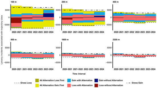
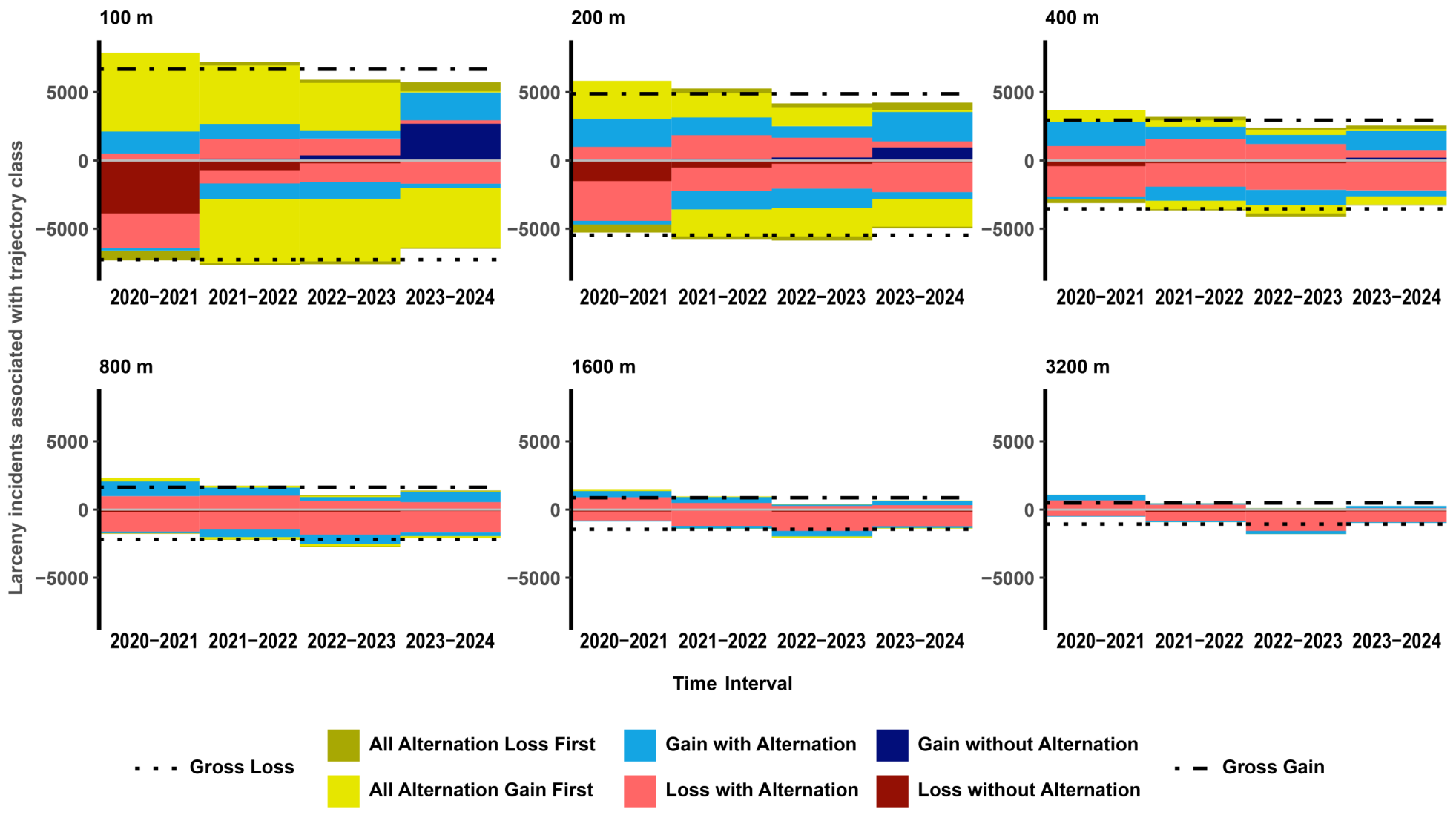
The six trajectories with changes of the spatio temporal dataset of larceny presence in Mexico City are analyzed for various resolutions: 100, 200, 400, 800, 1600, and 3200 m per cell. As a first salient result, we present the trajectory plots in Figure 5.
Figure 5.
Trajectory plots for different resolutions.
Figure 5 shows the sensitivity of Gain, Loss and the six trajectories to changes in resolution. The decrement is observed primarily by the reduction of the absolute values of Gross Loss, and Gross Gain.
The most prominent trajectory at 100 m is the All Alternation Gain First, which almost disappears at a resolution of 1600 m. According to this result, this component is the most sensitive to resolution. The second most sensitive is Gain without Alternation and Loss without Alternation, which almost disappears at a resolution of 400 m. In contrast, Gain with alternation and Loss with Alternation are the most robust trajectories, fluctuating across resolutions without vanishing completely. This analysis reveals the spatial distances at which displacements occur and produce alternation. For example, the trajectory plot at 3200 m shows that All Alternation categories vanish because the spatial displacements are confined within the 3200 m square region.
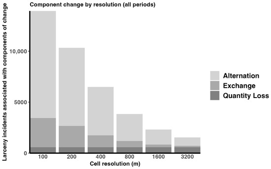
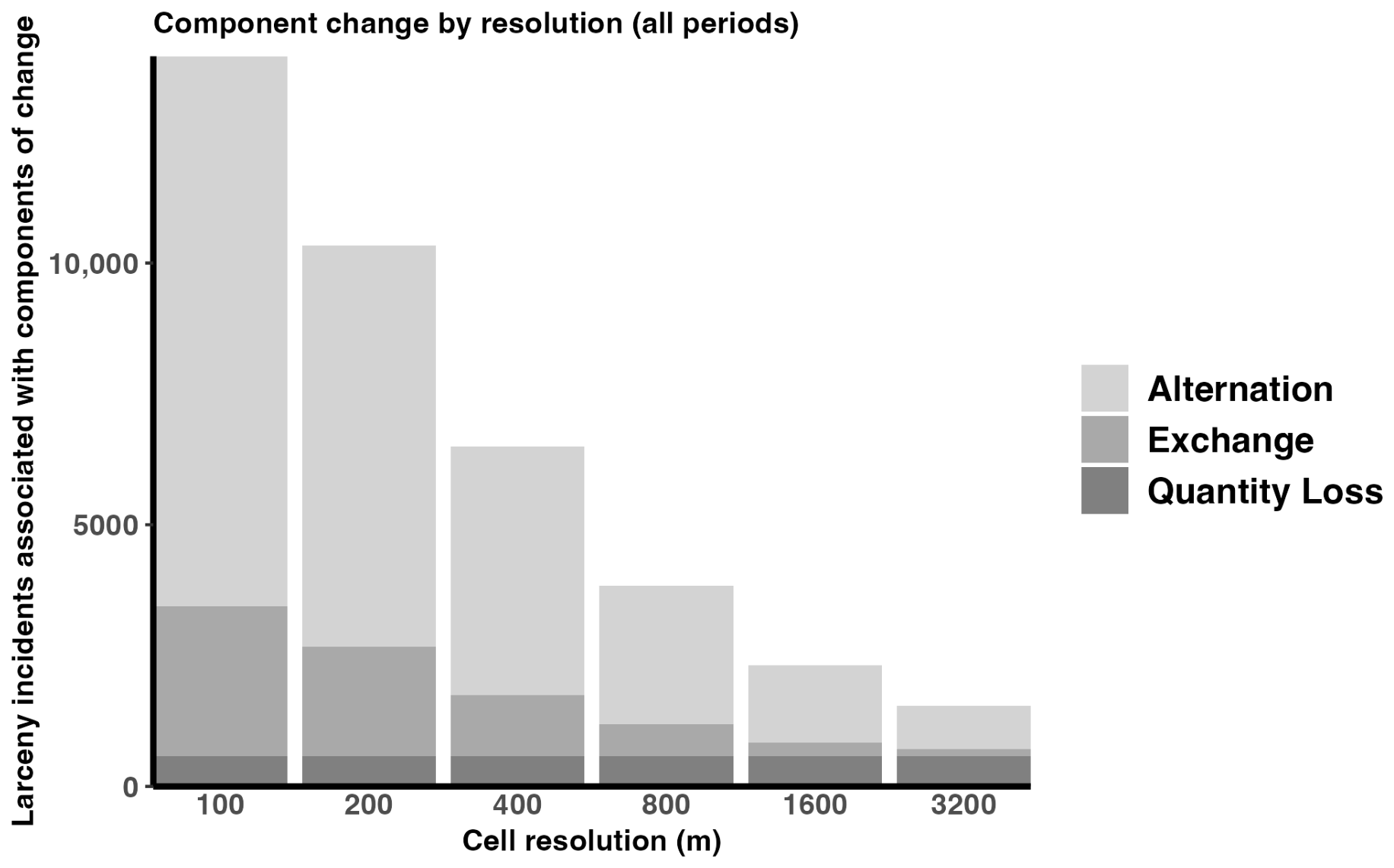
Figure 6 presents the Alternation, Exchange, and Quantity components for the time series from 2020 to 2024 as a function of resolution. It also reveals how rapidly the Alternation and Exchange components decrease. Quantity Loss is invariant when U is constant. As mentioned previously, we set for all resolutions to obtain results in terms of larceny events. Although this is an expected behavior, the analysis focuses on identifying the evolution of these components presented in Figure 7. Note, however, that when considering non-negative continuous variables and U is set to ‘unified’, the Quantity component is affected by changes in spatial resolution because adds count values to the calculated unified region instead of computing the union of observations that have presence of the category at any time point.
Figure 6.
Stack plots of Alternation, Exchange and Quantity at different resolutions.
Figure 7.
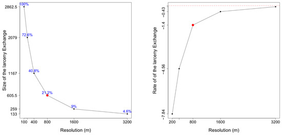
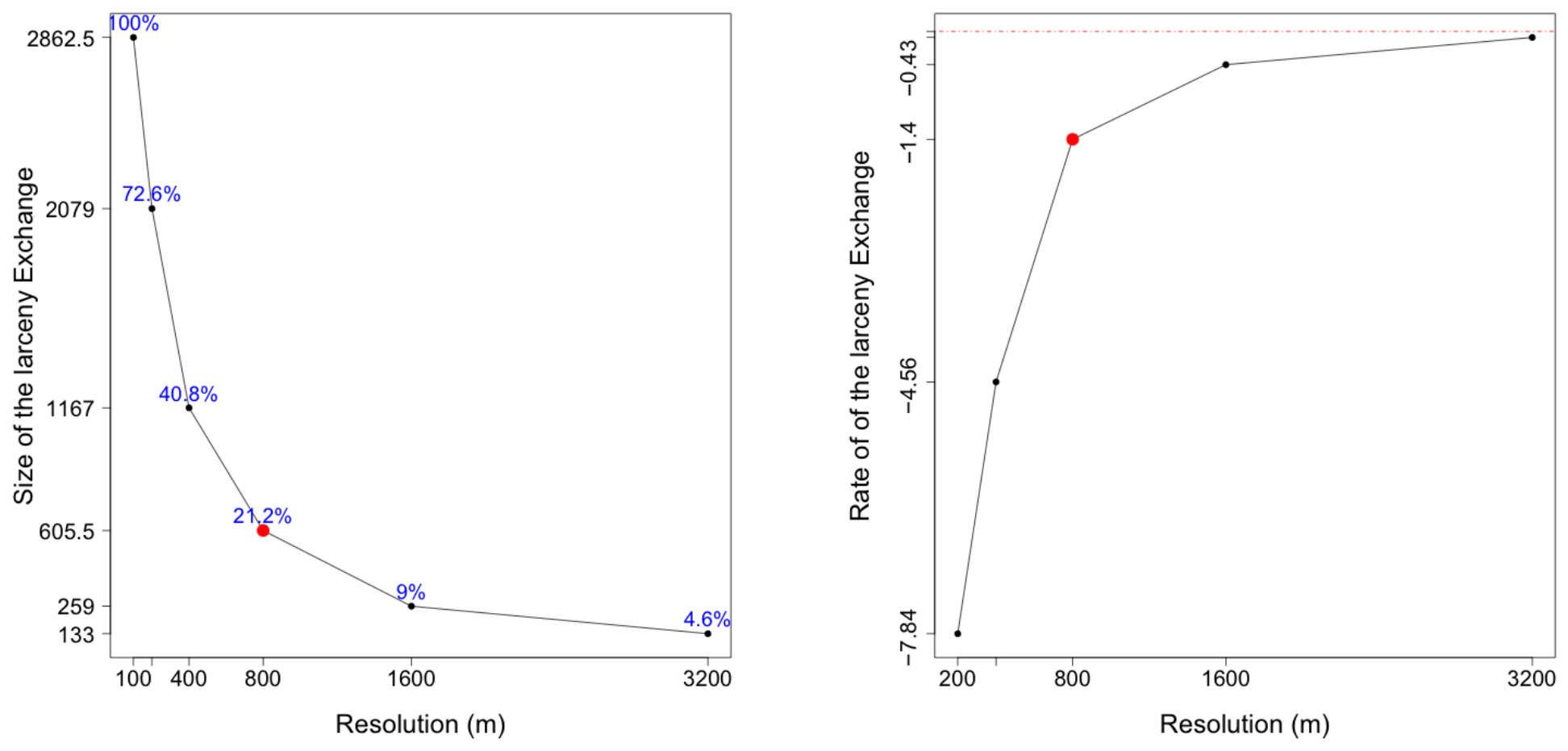
On the (left), the size of the larceny exchange with its percentage for the study region at different resolutions. On the (right), the first differences are presented to highlight the Exchange rates between consecutive resolutions. The red dotted line represents no variation. The red dot indicates the selected resolution.
Figure 7 presents the resolution analysis of the Exchange component. The plot shows that the Exchange component decreases following a similar function to the exponential decay. This figure indicates that the spatial concentration of larceny displacements as a function of resolution follows an exponential pattern.
4.2. Analysis of the Monotonic Trend of the Trajectories
In this subsection we present the results of the strength of the monotonic trend across the classified trajectories. While these were calculated for all resolutions, for the sake of space we only present the ones at 800 m. This was the chosen resolution to show results because the Exchange component becomes less sensitive after this resolution, as can be attested by looking at Figure 6 and Figure 7. Furthermore, if one considers the average rate of change of the exchange component with respect to resolution, moving from 400 m to 800 m reduces the Exchange value nearly in half (~48%), indicating a large amount of exchange reduction at this scale. From 800 m onward exchange reduction is much less than at previous resolutions and, thus, this can be interpreted as the resolution where exchange starts to stabilize.
We inspect if it is possible to identify areas of controlled and uncontrolled larceny activity using these results.
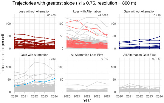
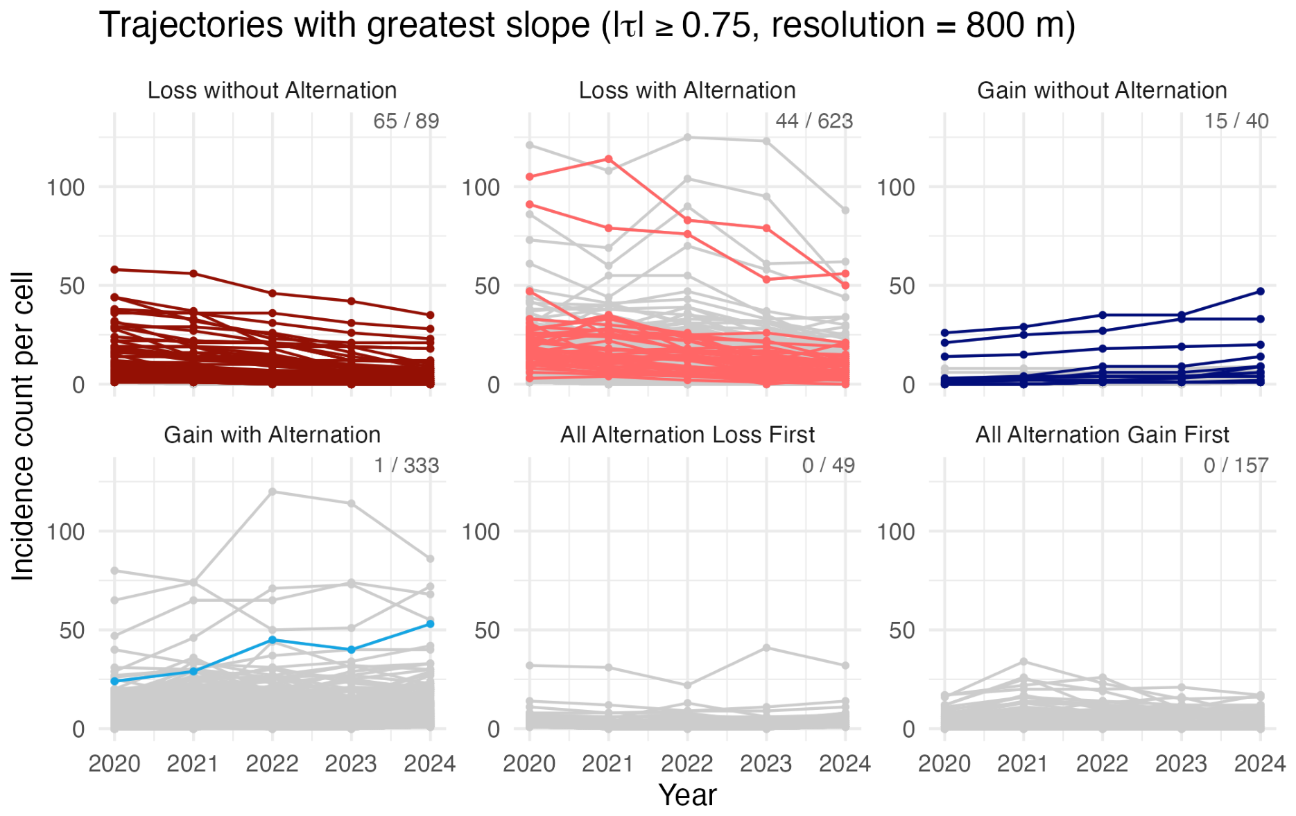
Figure 8 presents 1291 trajectories excluding the Stable Absence and Stable Presence classes that, by definition, do not show any trend, highlighting 126 trajectories with an absolute value of the coefficient greater than 0.75.
Figure 8.
Parallel plot of trajectories at 800 m resolution. Highlighted trajectories show strong monotonic trends. Colors correspond to those in Figure 5.
Among the trajectories classified as Loss without Alternation and Loss with Alternation, 110 out of 709 have values above the threshold, which indicate the number of controlled areas with a strong negative monotonic trend in larceny activity. Conversely, among the trajectories classified as Gain with Alternation and Gain without Alternation, only 16 out of 173 have values above the threshold, suggesting a reduced number of areas with uncontrolled larceny activity that should be prioritized for further investigation. The remaining classes All Alternation Loss First and All Alternation Gain First do not show trajectories with values above the threshold, indicating weak monotonic trends. It is important to notice that, independently of the trend magnitude, this information is useful to identify areas that must be prioritized in case the objective is to reduce the larceny.
It is important to remark that Gain With Alternation has only 1 out of 333 strong increasing monotonic trajectory, All Alternation Loss First and All Alternation Gain First did not have any strong direction, suggesting that the larceny events variations are likely to be uncorrelated without any visible temporal association.
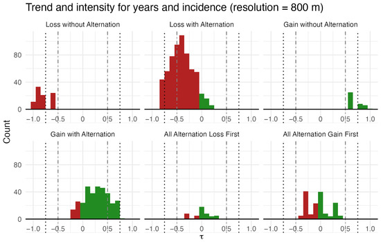
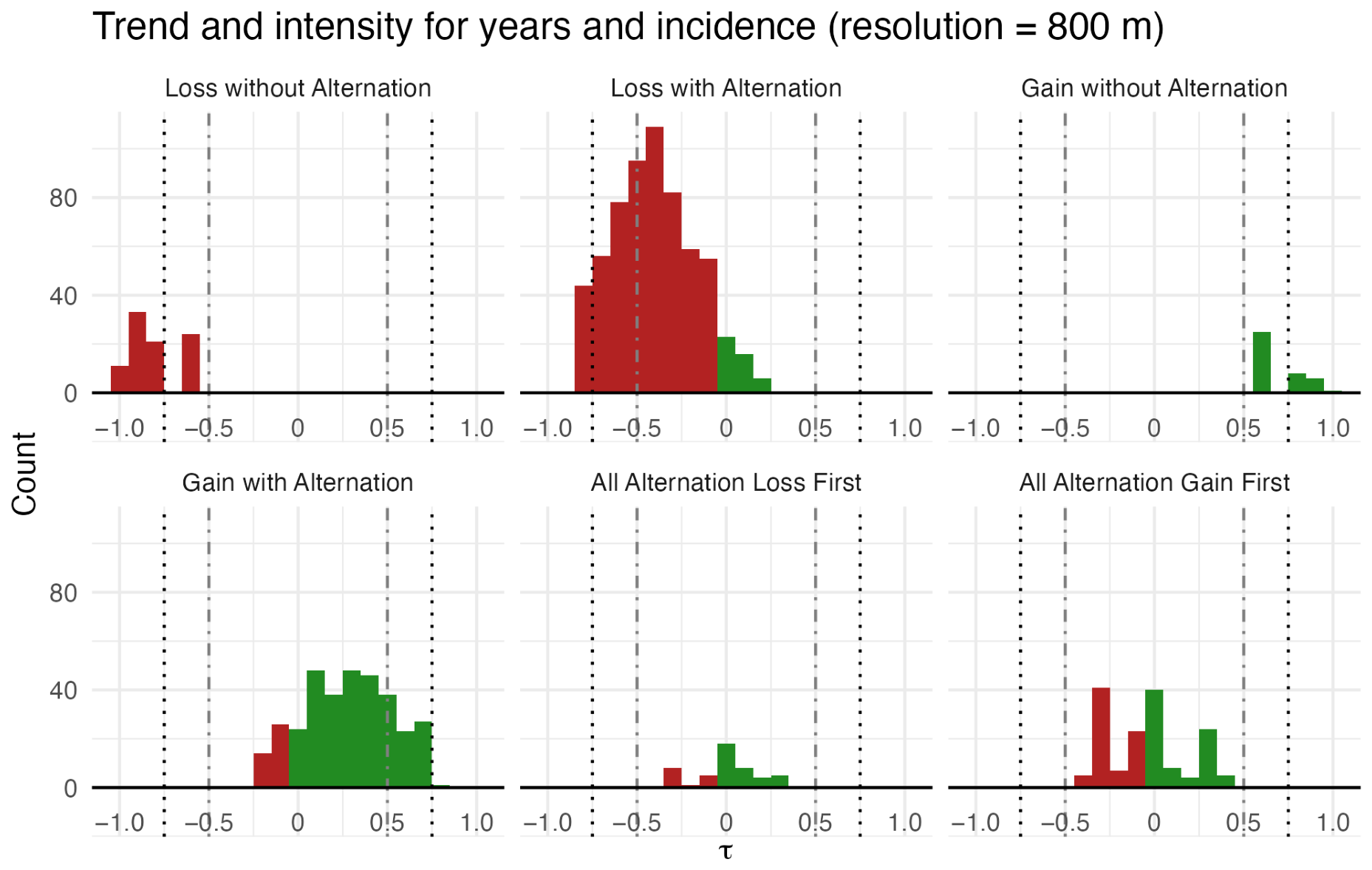
Figure 9 shows a dual histogram of frequencies for each trajectory class. The horizontal axis shows the value of , which ranges from −1 to 1. The vertical axis is the number of trajectories with a specific coefficient. The green bars are associated with the distribution of positive values of and the red ones with the distribution of negative values of . Reference values of ±0.5 and ±0.75 are indicated with vertical dashed lines.
Figure 9.
Distribution histogram of values for each of the six trajectory classes. Reference values of ±0.5 and ±0.75 are indicated with vertical dashed lines.
In the histogram, the behavior of the Loss without Alternation class is expected to have only negative coefficients for all trajectories. The red negative bars are in agreement with the gross expected behavior but the strengths of the negative direction for this trajectories are between −0.5 and −1. In the case the of Loss with Alternation class, the expected behavior is to observe more negative coefficients than positive ones. The histogram shows that the strength of most trajectories with negative direction are concentrated between −0.4 and −0.5 with a few ones with positive, albeit weak, strength. For the Gain without Alternation case, the expected behavior is the opposite with respect to the Loss without Alternation one. It shows that most of the trajectories have a coefficient of 0.6, corroborating few increasing trajectories but with considerable strength. At this point we can say that the Loss with Alternation categories are more frequent and with slightly higher direction strength than the Gain without Alternation ones. Moving on to the Gain with Alternation trajectories, a general inverse distribution with respect to the Loss with Alternation case is expected. Most trajectories in this category have positive coefficient values between 0.0 and 0.75, with some trajectories presenting negative but small coefficients ranging from −0.1 to −0.25. Then, for the All Alternation Loss First class, the strength is weak for both positive and negative coefficients, showing trajectories with coefficients below 0.5 and −0.5. In this class we observe non dominant number of positive and negative coefficients. Lastly, for the All Alternation Gain first class, there is a similar balance with respect to the All Alternation Loss First case. This category contains more trajectories with weak direction strength in both, positive and negative directions, like with All Alternation Loss First.
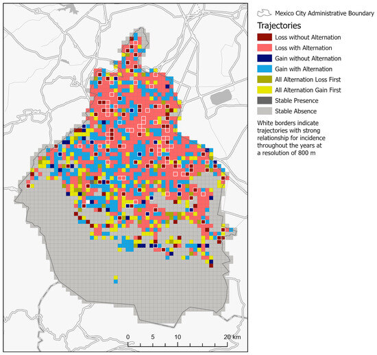
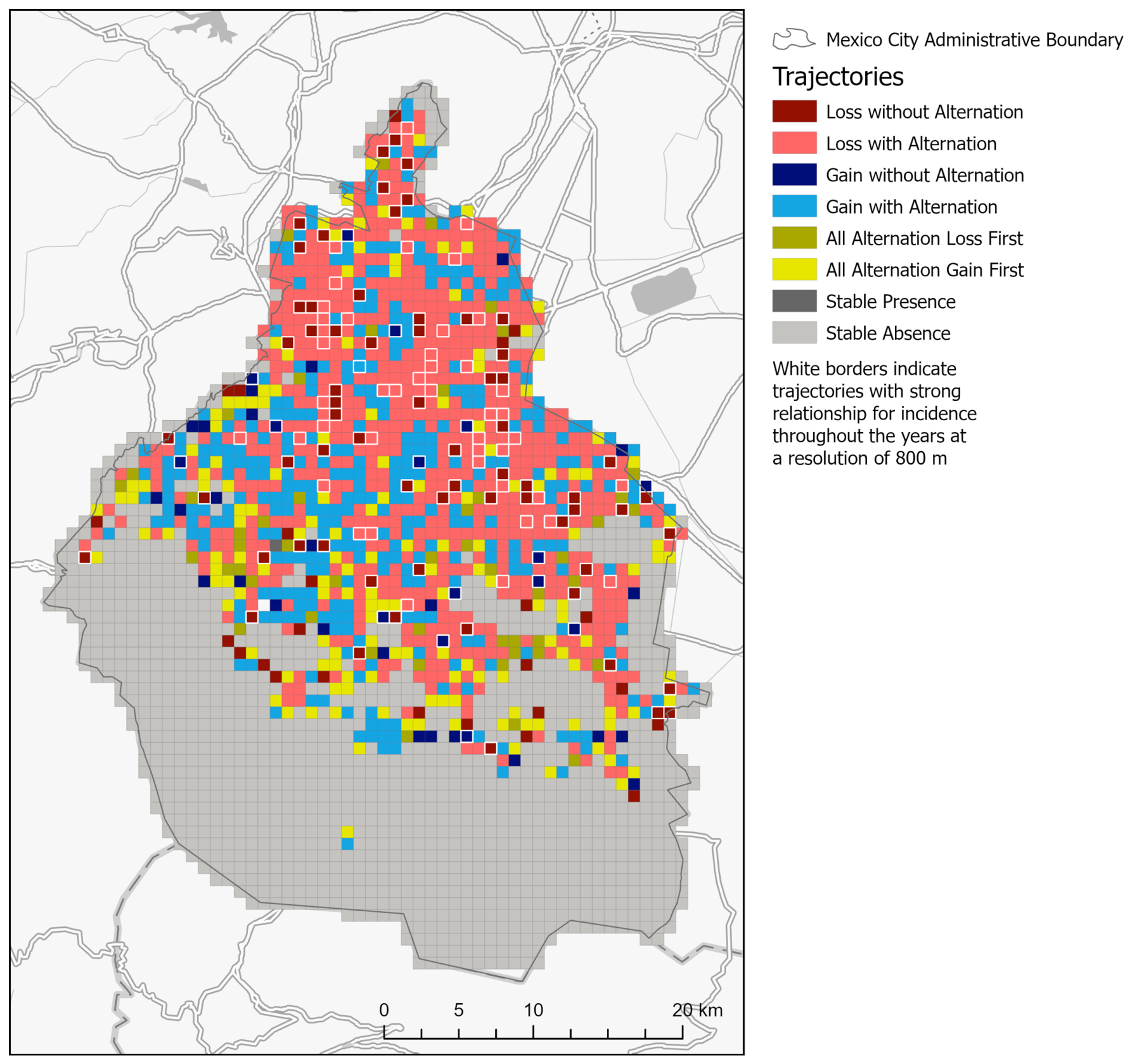
Figure 10, is the most important one of this study, as it aims at summarizing all the results. It presents the georeferenced trajectories at a resolution of 800 m per cell extended with information of the coefficient. This map is useful to indicate areas with minor spillover effect where larceny mitigation strategies should be aimed.
Figure 10.
Trajectory map at a resolution of 800 m that highlights trajectories with the strongest monotonic trend of larceny incidence with time.
In this map, trajectories with monotonic trend values of are indicated with white borders around cells. This map reveals areas where larceny is an increasing public safety concern, while some regions present a strong consistent decrement of larceny events.
At this resolution, only 13 out of 1297 trajectories present strong monotonic increase of larceny events that must be looked into and are distributed in the southern portion of the city. Possible larceny contention strategies seem to be successful in 99 regions out of 1297, as observed by the strong negative direction of the Loss with Alternation and Loss without Alternation classes. For the rest of the trajectories, the association with consistent decrement of larceny activity is relatively weak.
The overall decrease in larceny incidence associated with the observed spatial displacement patterns warrants further investigation. The study was not designed to unveil mechanisms that could contribute to the observed pattern (like changes in local environmental conditions, policing strategies, socioeconomic dynamics, offender adaptation or displacement processes). Potential implications of spatially targeted interventions are beyond the scope of the current descriptive research. It is not the intention to attempt to establish causal relationships, but it is recognized as an interesting direction of future research.
5. Conclusions
In this work we proposed the application of resolution analysis to identify the concentration of spillover effects through the Exchange component, enhancing trajectory analysis with the strength of the monotonic trend analysis with Kendall’s coefficient, and describing the distribution of the trajectories of each class by using dual histograms to nuance the hard classification of the trajectories.
Used jointly, they are useful to generate the final map that highlights areas where anti-larceny campaigns could be implemented. The analysis of the size of the Exchange component in terms of the resolution gives information regarding the characteristics of the location of the larceny problem. It is expected to observe an decrease in exchange if the spillover is somewhat localized in bounded regions. One limitation of the trajectory analysis approach is that it does not explicitly model spatial dependence. More research is needed to further develop and strengthen the framework.
Parallel plots and histograms are complementary visual methods, where the first one presents the trajectories in a qualitative way, while the histograms show the distribution of all trajectories in each class. Parallel plots are useful to identify and visualize trajectories that present strong monotonic trend of larceny incidents. Overall, the methodology proved to be useful in describing and highlighting important regions with problems regarding reduction of larceny events and also helps showing regions with important decrement of this crime.
The resolution analysis of the Exchange component provides a fast, useful, and intuitive general approximation of the area that confines a proportion of larceny displacements.
The method is limited to quantifying the displacements inside an area but fails in providing information regarding the displacement direction of the larceny. In this sense, a method to describe the probable starting and ending points of larceny displacements is necessary to describe source and destination of the displaced larceny. In this regard an option could be the characterization of change with networks. Examples of these applications are found in [29,30], which identify a spatial relation of change using complex networks. Since the distribution of the Exchange component across the square tessellations is heterogeneous, it may be advantageous using graphical methods to identify regions with similar behavior.
We observed that the computation of the unified size is valid just for binary raster maps by using the Equation (1) presented in [4]. For raster maps with positive integers or continuous variables, it is not equivalent to compute the unified size of a site.
More research is needed to analyze the implications of computing the unified size for raster maps with continuous values. One alternative could be transform the raster map of continuous values to a binary map before calculating the unified region and then multiply the number of cells of the unified size by the appropriate scale.
Author Contributions
Conceptualization, R.L.-F. and R.T.-M.; methodology, R.T.-M., R.L.-F., and C.C.-C.; software, R.T.-M.; validation, R.T.-M., R.L.-F., and C.C.-C.; formal analysis, R.T.-M., R.L.-F., and C.C.-C.; investigation, R.T.-M., R.L.-F.; resources, R.T.-M.; data curation, R.T.-M.; writing—original draft preparation, R.L.-F.; writing—review and editing, R.T.-M. and R.L.-F.; visualization, R.T.-M. All authors have read and agreed to the published version of the manuscript.
Funding
This research received no external funding.
Data Availability Statement
The data used in this study were derived from Portal de Datos Abiertos de la CDMX - Carpetas de Investigación (acumulado 2016–2024) available at https://datos.cdmx.gob.mx/dataset/carpetas-de-investigacion-fgj-de-la-ciudad-de-mexico/resource/48fcb848-220c-4af0-839b-4fd8ac812c0f, accessed on 20 September 2024. Processed data will be made available by the authors on request.
Conflicts of Interest
The authors declare no conflicts of interest.
References
- Mátyás, S. Crime Geography. Available at REAL (Repository of the Hungarian Academy of Sciences). 2024. Available online: https://real.mtak.hu/204407/1/Crime_Geography_MatyasSzabolcs.pdf (accessed on 20 January 2025).
- Qazi, N.; Wong, B.W. An interactive human centered data science approach towards crime pattern analysis. Inf. Process. Manag. 2019, 56, 102066. [Google Scholar] [CrossRef] [Scilit]
- Bilintoh, T.M. timeseriesTrajectories. 2024. Available online: https://github.com/bilintoh/timeseriesTrajectories (accessed on 15 January 2025).
- Bilintoh, T.M.; Pontius, R.G., Jr.; Zhang, A. Methods to compare sites concerning a category’s change during various time intervals. Gisci. Remote Sens. 2024, 61, 2409484. [Google Scholar] [CrossRef] [Scilit]
- Pontius, R., Jr.; Bilintoh, T.; Oliveira, G.; Shimbo, J.Z. Trajectories aof Losses and Gains of Soybean Cultivation During Multiple Time Intervals in Western Bahia, Brazil. In Proceedings of the Anais da Space Week Nordeste 2023, Fortaleza, Brazil, 14–20 August 2023. [Google Scholar]
- Barbosa, B.; Gonçalves, A.; Oliveira, S.; Viana, C.M. Mapping Long-Term Wildfire Dynamics in Portugal Using Trajectory Analysis (1975–2024). Land 2025, 14, 1872. [Google Scholar] [CrossRef] [Scilit]
- Solórzano, J.V.; Mas, J.F.; Ramírez-Mejía, D.; Gallardo-Cruz, J.A. Long-Term Trajectory Analysis of Avocado Orchards in the Avocado Belt, Mexico. Land 2025, 14, 1792. [Google Scholar] [CrossRef] [Scilit]
- Longford, N.T. Longitudinal and Time-Series Analysis. In Studying Human Populations: An Advanced Course in Statistics; Springer: New York, NY, USA, 2008; pp. 335–370. [Google Scholar] [CrossRef] [Scilit] [PubMed]
- Abbott, A. Sequences of social events: Concepts and methods for the analysis of order in social processes. Hist. Methods 1983, 16, 129–147. [Google Scholar] [CrossRef] [Scilit]
- Mills, M. Sequence Analysis. In Introducing Survival and Event History Analysis; SAGE Publications Ltd.: London, UK, 2012; Chapter 11; pp. 213–226. [Google Scholar] [CrossRef] [Scilit]
- Ritschard, G.; Studer, M. (Eds.) Sequence Analysis and Related Approaches; Life Course Research and Social Policies; Springer International Publishing: Cham, Switzerland, 2018; Volume 10. [Google Scholar] [CrossRef] [Scilit]
- Nagin, D.S.; Tremblay, R.E. Analyzing developmental trajectories of distinct but related behaviors: A group-based method. Psychol. Methods 2001, 6, 18–34. [Google Scholar] [CrossRef] [PubMed]
- Weisburd, D.; Bushway, S.; Lum, C.; Yang, S.M. Trajectories of Crime at Places: A Longitudinal Study of Street Segments in the City of Seattle. In Quantitative Methods in Criminology; Routledge: London, UK, 2017; pp. 443–481. [Google Scholar] [CrossRef] [Scilit]
- Weisburd, D. The law of crime concentration and the criminology of place. Criminology 2015, 53, 133–157. [Google Scholar] [CrossRef] [Scilit]
- Grubesic, T.; Mack, E. Spatio-Temporal Interaction of Urban Crime. J. Quant. Criminol. 2008, 24, 285–306. [Google Scholar] [CrossRef] [Scilit]
- Alegre-Mondragón, A.J.; Silva-Arias, C. Effects of COVID-19 in Mexico City: Street Robbery and Vehicle Theft Spatio-Temporal Patterns. In Lecture Notes in Geoinformation and Cartography; Springer: Cham, Switzerland, 2022; pp. 195–205. [Google Scholar] [CrossRef] [Scilit]
- Chainey, S.P.; da Silva, B.F.A. Examining the extent of repeat and near repeat victimisation of domestic burglaries in Belo Horizonte, Brazil. Crime Sci. 2016, 5, 1. [Google Scholar] [CrossRef] [Scilit]
- Hu, T.; Zhu, X.; Duan, L.; Guo, W. Urban crime prediction based on spatio-temporal Bayesian model. PLoS ONE 2018, 13, e0206215. [Google Scholar] [CrossRef] [Scilit] [PubMed]
- Kronkvist, K.; Borg, A.; Boldt, M.; Gerell, M. Predicting Public Violent Crime Using Register and OpenStreetMap Data: A Risk Terrain Modeling Approach Across Three Cities of Varying Size. Appl. Spat. Anal. Policy 2024, 18, 9. [Google Scholar] [CrossRef] [Scilit]
- Harinam, V.; Bavcevic, Z.; Ariel, B. Spatial distribution and developmental trajectories of crime versus crime severity: Do not abandon the count-based model just yet. Crime Sci. 2022, 11, 14. [Google Scholar] [CrossRef] [Scilit]
- Shiode, S. Street-level Spatial Scan Statistic and STAC for Analysing Street Crime Concentrations. Trans. Gis 2011, 15, 365–383. [Google Scholar] [CrossRef] [Scilit]
- Instituto Nacional de Estadística y Geografía. Censo de Población y Vivienda 2020. 2020. Available online: https://www.inegi.org.mx/programas/ccpv/2020/ (accessed on 20 February 2025).
- Schiavina, M.; Alessandrini, A.; Melchiorri, M.; Dijkstra, L. PGHS-WUP-MTUC R2025A–GHS-WUP Multitemporal Urban Centres, Obtained from the Degree of Urbanisation Grids (GHS-WUP-DEGURBA R2025A) and Linked Across Epochs, Multitemporal (1950–2100); European Commission, Joint Research Centre Data Catalogue: Bruxelles, Belgium, 2026. [Google Scholar] [CrossRef]
- Instituto Nacional de Estadística y Geografía. Encuesta Nacional de Victimización y Percepción sobre Seguridad Pública (ENVIPE). 2024. Available online: https://www.inegi.org.mx/programas/envipe/ (accessed on 20 February 2025).
- United Nations Development Programme (UNDP). Human Development Report for Latin America and the Caribbean 2013–2014: Citizen Security with a Human Face; Technical Report; United Nations Development Programme: New York, NY, USA, 2013. [Google Scholar]
- Mendoza, A.L.R. Miedo en las calles: Principal emoción de la inseguridad pública delictiva. Un estudio criminológico y de género. Rev. IUS 2014, 8, 81–100. [Google Scholar]
- Fiscalía General de Justicia. Carpetas de Investigación FGJ. 2024. Available online: https://datos.cdmx.gob.mx/dataset/carpetas-de-investigacion-fgj-de-la-ciudad-de-mexico (accessed on 20 September 2024).
- Kendall, M.G. Rank Correlation Methods, 4th ed.; Charles Griffin: New York, NY, USA, 1976. [Google Scholar]
- Pichardo-Corpus, J.; Solano Lamphar, H.; Lopez-Farias, R.; Delgadillo Ruiz, O. Spatio-temporal networks of light pollution. J. Quant. Spectrosc. Radiat. Transf. 2020, 253, 107068. [Google Scholar] [CrossRef] [Scilit]
- Hernández-Paniagua, I.Y.; López-Farías, R.; Pichardo-Corpus, J.A. Application of network theory to study the spatio-temporal evolution in the ozone weekend effect in urban areas. Atmósfera 2022, 35, 521–543. [Google Scholar]

Disclaimer/Publisher’s Note: The statements, opinions and data contained in all publications are solely those of the individual author(s) and contributor(s) and not of MDPI and/or the editor(s). MDPI and/or the editor(s) disclaim responsibility for any injury to people or property resulting from any ideas, methods, instructions or products referred to in the content. |
© 2026 by the authors. Licensee MDPI, Basel, Switzerland. This article is an open access article distributed under the terms and conditions of the Creative Commons Attribution (CC BY) license.