Abstract
Climate change intensifies the challenge of elevated temperatures in dense urban areas, notably in Seoul, South Korea. This study investigates the effects of land use and urban form on summer air temperatures by leveraging Seoul’s city-wide Smart Seoul Data of Things sensor network. Using spatial regression models and temperature data collected during July and August 2021, the analysis identifies key environmental factors associated with urban heat dynamics. The results show that medium- and high-density residential areas, industrial zones, and roads consistently increase temperatures, while greenery, taller buildings, and greater urban porosity contribute to cooling effects. The findings highlight the need for urban planning strategies that expand green spaces, promote vertical development with attention to ventilation, and reconfigure built environments to enhance thermal comfort. This study provides robust empirical insights and offers evidence-based recommendations for climate-responsive urban planning and policies in Seoul and similar high-density cities worldwide.
1. Introduction
As acknowledged by the Intergovernmental Panel on Climate Change, the world currently faces temperatures rising at a rate never experienced before [1]. Cities, in particular, experience higher temperature levels and faster warming trends, and discussions on how the built environment influences surface or near-ground temperature in cities are advancing [2,3].
Researchers worldwide are actively investigating the impact of urban built environments on thermal conditions across various scales. At a broader level, numerous studies examine the effects of different land use and land cover (LULC) patterns to guide policy decisions for metropolitan areas. These investigations consistently report that built-up areas and impervious surfaces tend to experience higher temperatures [4,5,6]. In contrast, vegetated zones and water bodies generally maintain lower temperatures [7,8,9]. This growing body of research underscores the critical role of urban planning and design in mitigating heat-related challenges in cities, highlighting the potential for strategic LULC management to create more thermally comfortable urban environments [10,11,12,13].
At the urban scale, researchers frequently examine the effects of land use to provide insights for local comprehensive planning. Their findings consistently show that industrial and commercial areas with higher density are more inclined to elevate temperatures, whereas residential areas and green spaces tend to have a cooling effect, lowering temperatures [3,14,15,16,17]. Another area of research at the same scale focuses on diverse urban forms and geometries, such as floor area ratio, building density, aspect ratio, and sky view factor, to understand their impact on thermal conditions [18,19,20,21,22,23]. Additionally, there is a substantial body of research dedicated to studying the cooling effects of green elements, including small open spaces and green roofs, which are integrated into urban and building designs [24,25,26].
In addition to the range of spatial scales at which these studies are conducted, there are mainly two sources of temperature data utilized [27]. Firstly, most LULC studies at broader scales heavily rely on remotely sensed data, typically collected by satellites like Landsat 8 and Sentinel [10,12,28,29]. These data not only present LULC information but also provide land surface temperature estimates across wider geographical territories so as to make possible investigation of the relationship between the two. Secondly, studies at more urban or smaller scales usually depend on near-ground air temperatures collected at weather stations or by using portable measuring devices [3,30,31,32]. They combine land use or urban form information collected from public sources with temperature data recorded for longer periods and identify relationships between them.
Using remotely sensed data is widely favored for several reasons. Its primary strength lies in its extensive coverage and the broad scope it can effectively manage [29]. With the rising prevalence of higher resolutions in research applications, there is growing accessibility to land surface information that offers a wealth of detailed data [32,33]. It also facilitates prolonged monitoring of specific areas, primarily concerning their land surface or environmental conditions, allowing for easy detection of changes over time [34,35].
On the other hand, remotely sensed data have inherent disadvantages. Their accessibility is frequently contingent upon prevailing weather patterns and daily fluctuations in environmental conditions, generating data gaps [29,36]. The generated LULC information may be too simplified or superficial to be applied to local planning practice and policymaking [37]. The whole process depends heavily on certain classification methods based on their own algorithms but is subject to incurring errors [38,39].
The primary advantage of using near-surface air temperatures provided by the public sector is their authenticity. These are actual readings collected with calibrated devices rather than retrieved or generated values. Consequently, these measured temperatures are likely to be more reliable and precise. However, the main drawback is the scarcity of data on a larger scale [40,41,42], which significantly limits the ability to cover wider territories comprehensively. To address these limitations, researchers have explored alternative approaches. Some adopt crowdsourced temperature data [41,43], leveraging the potential of citizen science. Others combine measured data with remotely sensed information [42,44], aiming to bridge the gap between accuracy and coverage
An optimal approach to measuring near-surface air temperatures involves deploying a high-density horizontal network of temperature sensors, enabling more precise readings across a broader geographical area. The Smart Seoul Data of Things (S-DoT) initiative in Seoul, South Korea, exemplifies this approach and represents a significant advancement in urban environmental monitoring. Launched in 2019, the Seoul Metropolitan Government utilizes the S-DoT Internet of Things (IoT) network to facilitate data-driven policymaking. As of late 2022, this ambitious project deploys over a thousand sensors throughout the city. This extensive network enables the systematic collection and analysis of diverse environmental data.
Based on what has been discussed so far, we investigate to what extent the thermal environment is affected by land use and urban form variables, specifically daily, daytime, and nighttime variations in summer air temperatures across Seoul, using high-resolution data from more than 1000 S-DoT sensors distributed city-wide. It adopts spatial regression models to empirically investigate these effects. The insights derived from this study can offer valuable advantages not only to the planners and policymakers of Seoul but also to those in numerous cities globally. This information is particularly beneficial for those navigating strategies and measures to address escalating temperatures within urban settings. Additionally, researchers interested in examining the impact of the built environment on temperatures can find value in the utilization of a dense horizontal network of temperature sensors that spans a substantial urban area like Seoul.
2. Case Context
Seoul (37°33′36″ N 126°59′24″ E), the capital city of South Korea with a population over nine million, stands out as one of the world’s fastest-warming urban centers. This phenomenon is predominantly attributed to the extraordinarily high concentrations of population and industry, exacerbated by the densely populated urban environment that accommodates them [3,45,46,47]. As Figure 1 presents, Seoul’s annual mean temperature has surged from 11.5 °C in 1971 to 14.9 °C in 2024. This corresponds to a warming rate of 0.64 °C per decade, more than triple the global average of 0.18 °C per decade since 1981 [48]. Notably, Seoul’s summer mean temperatures rise at an even more pronounced rate of 0.65 °C per decade, raising significant concerns about the potential negative impacts on the local community. The most remembered heatwaves occurred in 1994 and 2018 prior to 2024 which recorded the highest annual and summer mean temperatures to date. Seoul’s annual mean temperature is projected to reach 19.8 °C by the end of this century under the SSP5-8.5 scenario [49].
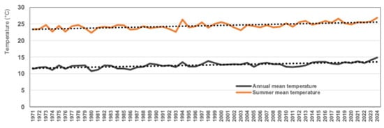
Figure 1.
Annual and summer mean temperatures of Seoul, South Korea, between 1971 and 2024 (data source: Open MET Data Portal; https://data.kma.go.kr/, accessed 5 January 2025).
South Korea’s temperature changes are monitored by a network of over 600 automated weather stations nation-wide, with 30 strategically placed in Seoul, creating one of the densest urban weather station networks [50]. For decades, these stations have collected real-time data on various meteorological parameters at intervals as frequent as every minute. These data have significantly contributed to research on South Korea’s local climate and informed local policymaking and planning initiatives [32,51,52].
In 2019, the city’s capacity to collect climate data advanced to a new level. The Seoul Metropolitan Government embraced smart city initiatives with the launch of the city-wide S-DoT—an IoT network designed for data-driven policymaking and public services. This network systematically collects data on various environmental conditions, including temperature, humidity, air pollution, illuminance, noise, vibration, ultraviolet rays, wind speed and direction, and head counts as shown in Figure 2. Each station is placed 2 to 4 m above ground, usually on lighting or traffic poles that can be regularly maintained by the local government. Data are measured every two minutes for environmental information [53].
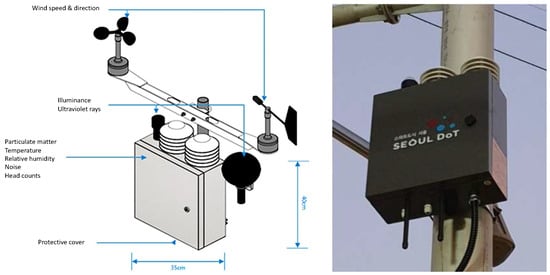
Figure 2.
An S-DoT station (images courtesy of the Seoul Metropolitan Government).
In 2019, 850 S-DoT stations were first deployed, followed by an additional 250 in 2020. As of late 2021, approximately 1100 S-DoT stations are operational across the city, as illustrated in Figure 3, actively enhancing its extensive network. These stations are strategically distributed throughout Seoul, representing a wide spectrum of spaces within the city, from commercial centers to residential areas. Recent empirical studies using S-DoT data consistently demonstrate the high level of accuracy [54,55].
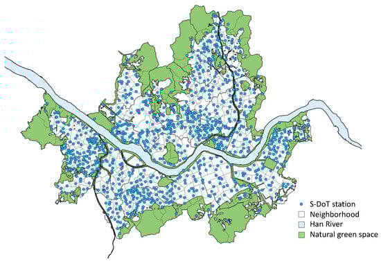
Figure 3.
Location of S-DoT stations in Seoul.
3. Materials and Methods
3.1. Materials
Based on our research purpose, we hypothesize that the surrounding land use and urban form conditions around each S-DoT station affect the temperature measured at the station. While some studies adopt fixed buffer distances around each measurement location, optimal buffer sizes can be used to reflect the extent of land use and urban form influence around each S-DoT station. We employ “A Distance Decay REgression Selection Strategy” (ADDRESS) [56,57] to select the buffer distances. This method identifies buffer distances with the strongest correlations relative to other variables and incorporates sensitivity analysis for statistical validation to enhance model performance. Based on similar studies [3,58,59], our candidate buffer distances are 50, 100, 200, 300, 400, and 500 m.
Table 1 provides a comprehensive overview of the dependent and independent variables used in this study, including their units and data sources. The dependent variables include mean daily temperature, mean daytime temperature, and mean nighttime temperature, all measured in degrees Celsius for each S-DoT station. These temperature data are sourced from the Seoul Open Data Plaza (https://data.seoul.go.kr/, accessed 5 January 2025), which is run by the Seoul Metropolitan Government, specifically from its S-DoT database. We use data from exactly 1063 S DoT stations, all of which provided complete records, for the typical summer months of July and August in Seoul in 2021. This year was selected because it offered the most complete and reliable S-DoT dataset among recent summers. The mean daily temperature represents the average temperature over the entire two-month period. Following the standards of the Korea Meteorological Administration, the mean daytime temperature is measured from 9:01 AM to 6:00 PM, and the mean nighttime temperature is recorded from 6:01 PM to 9:00 AM the following day within the same period.

Table 1.
Dependent and independent variables.
The independent variables are categorized largely into land use and urban form, with data sourced from the National Spatial Information Portal (https://map.ngii.go.kr/, accessed 5 January 2025), operated by the National Geographic Information Institute of South Korea. The land use variables are mainly based on Seoul’s local zoning codes and are expressed in proportions within each of their optimal buffer distances around each S-DoT station. They include categories such as low-density residential, medium-density residential, high-density residential, low-density commercial, medium- and high-density commercial, industrial, greenery, and road (see Appendix A for basic floor area ratio limits for each land use type).
The urban form variables include the sky view factor, porosity, aspect ratio, roughness, road area, built-up area, building volume, and mean building height. We use data from building attribute records, road address data, and cadastral information, all sourced from the National Spatial Information Portal. Firstly, the sky view factor refers to the ratio of unobstructed sky space to the total overhead expanse, with values spanning from 0 to 1. Higher sky view factor values facilitate improved air circulation and heightened solar influence [60,61]. We use the Terrain Shading plugin in QGIS to compute the sky view factor. This computation generates an output image, the pixel values of which are subsequently transformed into point-based data, enabling the derivation of the sky view factor values corresponding to each S-DoT location. Secondly, porosity refers to the proportion of non-building volume to the total volume within a designated site, ranging from 0 to 1. As porosity increases, air circulation is enhanced and the thermal environment is affected [62,63]. Given the wide spatial coverage of S-DoT across Seoul, we adopt the methodology proposed by Gál and Unger [64] to establish criteria for determining the total unit volume. We calculate the total unit volume by multiplying a horizontal area of 100 m by 100 m by the maximum building height around each S-DoT. Porosity is calculated by subtracting the volume occupied by buildings from the total unit volume within the same space, as shown in Equation (1):
where is the non-building volume, is the volume of a grid cell calculated based on its area and the height of the tallest building within it, and is the volume of building . The aspect ratio represents the proportion of road width to building height, which defines the physical configuration of street canyons. It is also widely known to affect the microclimate [65,66]. Since usually a large number of buildings and roads surround each S-DoT Station, we average building heights and road widths and use the mean aspect ratio for analysis, following Tang et al. [67]. The built-up area ratio represents the total land area occupied by buildings divided by the total buffer area, and the floor area ratio refers to the total floor space occupied by buildings, also divided by the total buffer area. Mean building height is the average height of all buildings within the buffer. Roughness, defined as the standard deviation of building heights within a specified region, relates to building-induced friction that affects wind flow and the cooling effect of breezes. Among the urban form variables, we do not apply ADDRESS to the sky view factor and porosity to assess their inherent properties.
3.2. Methods
Our observation of the three dependent variables—mean daily temperature, mean daytime temperature, and mean nighttime temperature—suggests the existence of spatial autocorrelation, indicating the presence of systematic spatial variation in these variables. As a global spatial autocorrelation coefficient, Moran’s I value of the mean daily temperature, mean daytime temperature, and mean nighttime temperature is 0.352 (p < 0.001), 0.181 (p < 0.001), and 0.428 (p < 0.001), respectively. These recommend the use of spatial regression models to take into account the existence of spatial autocorrelation.
Machine learning has gained popularity across many academic disciplines that employ quantitative methods. However, it typically requires larger datasets to ensure strong model performance and accuracy, making our moderate sample size of just over 1000 less suitable. Moreover, despite its vast potential, machine learning is still considered to have limitations in handling spatial autocorrelation compared to more established techniques. As a result, spatial regression models continue to be widely used due to their solid theoretical foundation and proven effectiveness in spatial data analysis [68,69]. In this sense, the most commonly used models for forecasting temperatures in cities include the spatial lag model (SLM), which captures the spatial autocorrelation of the dependent variable, and the spatial error model (SEM), which accounts for the spatial autocorrelation of the error term [70,71]. The SLM and SEM can be expressed as in Equation (2) and Equation (3), respectively:
where is the dependent variable, is a spatial autocorrelation parameter, is the spatial weight matrix, is the matrix of independent variables, is the matrix of coefficients, and is the error term;
and where is the spatial autoregressive coefficient of the error term, is the spatial weight matrix, and is a vector of error terms.
We adopt several more measures to ensure the quality of our spatial regression models. We check the variation inflation factor (VIF) value for each independent variable to monitor the strength of correlations among the independent variables. We use the Breusch–Pagan test to check for heteroskedasticity and apply robust spatial regressions if necessary.
4. Results
4.1. Descriptive Statistics
Table 2, Table 3 and Table 4 present the descriptive statistics of the variables used in the analysis when the dependent variable is the mean daily temperature, mean daytime temperature, and mean nighttime temperature, respectively. The mean daily temperature fluctuates between 24.537 and 30.617 degrees Celsius, with an overall average of 28.524 degrees Celsius. During the day, temperatures typically vary from 20.202 to 32.874 degrees Celsius, with a mean value of 30.430 degrees Celsius, while at night, temperatures range from 18.150 to 29.334 degrees Celsius, averaging at 27.314 degrees Celsius. The tables provide the optimal distances derived for all independent variables, except for the sky view factor and porosity, using ADDRESS, along with their descriptive statistics. VIF values are also included. In all three cases, no collinearity among the variables is witnessed.
Table 2.
Descriptive statistics when the dependent variable is mean daily temperature.
Table 3.
Descriptive statistics when the dependent variable is mean daytime temperature.
Table 4.
Descriptive statistics when the dependent variable is mean nighttime temperature.
Figure 4 shows the spatial distribution of the three dependent variables—mean daily temperature, mean daytime temperature, and mean nighttime temperature—all generated through interpolation using the Kriging technique. The three distributions in the left column utilize Seoul’s 1063 S-DoT data, with red indicating higher values and green representing lower values, and are used for empirical analysis. They visually present areas with higher temperatures that are widely distributed in an elongated east–west direction within Seoul in all three cases.
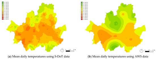
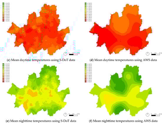
Figure 4.
Spatial distribution of Seoul’s mean daily temperatures (top), mean daytime temperatures (middle), and mean nighttime temperatures (bottom) in summer 2021 using S-DoT (left) and AWS data (right).
As a reference, we present temperature distributions in the right column, generated with data from the network of 28 sparsely located automated weather stations (AWSs) operated by the Korea Meteorological Administration. These have been utilized in a large number of previous studies that similarly focus on the relationship between the built environment and temperature in Seoul [3,45,46,72]. It is evident that the distributions generated by using S-DoT data, located in the left column, offer finer resolution than those in the right column, thereby allowing for higher levels of accuracy and reliability of the results.
4.2. Spatial Regression Results
Table 5 presents the spatial regression results with mean daily temperature as the dependent variable. Based on the statistical significance and size of the Lagrange Multiplier (LM) and robust Lagrange Multiplier (RLM) values for both the SLM and SEM, we find the former to be more appropriate. The Breusch–Pagan test for the SLM indicates the presence of heteroskedasticity. Therefore, we adopt the robust spatial lag model (RSLM) as the final model. Among the land use variables, medium-density residential (50 m), high-density residential (200 m), industrial (50 m), and road (500 m) present positive impacts on temperatures, indicating their role as significant heaters. Conversely, low-density residential (500 m) and greenery (500 m) are found to be significant coolers. Among the urban form variables, while built-up area ratio (200 m) and roughness (100 m) increase temperatures, porosity, floor area ratio (50 m), and mean building height (100 m) reduce temperatures.
Table 5.
Spatial regression results when the dependent variable is mean daily temperature.
The spatial regression results when the dependent variable is mean daytime temperature are shown in Table 6. Similarly, the LM and RLM values for the SLM and SEM suggest that the former is more applicable. The presence of heteroskedasticity from the Breusch–Pagan test result requires adoption of the RSLM as the final model. With respect to the land use variables, medium-density residential (50 m), high-density residential (200 m), industrial (50 m), and road (500 m) are identified as significant heaters, while low-density commercial (50 m) is found to be the only significant cooler. Regarding the urban form variables, sky view factor, built-up area ratio (50 m), and floor area ratio (500 m) increase temperatures, but mean building height (400 m) and roughness (50 m) decrease them.
Table 6.
Spatial regression results when the dependent variable is mean daytime temperature.
Table 7 shows the spatial regression results with mean nighttime temperature as the dependent variable. Again, we select the SLM as the more applicable model than the SEM based on their LM and RLM values and adopt the RSLM as the final model due to the presence of heteroskedasticity. Regarding the land use variables, medium-density residential (50 m), high-density residential (100 m), medium- and high-density commercial (50 m), industrial (50 m), and road (500 m) increase temperatures, while greenery (500 m) solely decreases them. Regarding the urban form variables, built-up area ratio (100 m) and roughness (100 m) operate as significant heaters, but the sky view factor, mean aspect ratio (500 m), floor area ratio (50 m), and mean building height (100 m) operate as significant coolers.
Table 7.
Spatial regression results when the dependent variable is mean nighttime temperature.
Table 8 summarizes the results of the three RSLM models, highlighting the key effects of statistically significant independent variables. Four land use types—medium-density residential, high-density residential, industrial, and roads—are consistently associated with temperature increases, with roads exerting the strongest effect and the other three showing similar magnitudes. Among the urban form variables, built-up area ratio consistently increases temperatures across all models, with an effect size comparable to that of roads. In contrast, mean building height is the only variable that consistently reduces temperatures in all models, with a clearer cooling effect during nighttime than daytime. Greenery is associated with lower temperatures during daily and nighttime periods, but not during the daytime. Medium- and high-density commercial areas show limited warming effects, primarily at night. Low-density residential and commercial areas, as well as porosity and mean aspect ratio, exhibit modest cooling effects. The sky view factor, floor area ratio, and roughness show mixed effects across the models.
Table 8.
Summary of three RSLM results.
5. Discussion
5.1. Land Use Impacts on Summer Air Temperatures
The empirical results provide diverse insights into the influence of land use on summer air temperatures in Seoul, South Korea, highlighting the need for further discussion. Foremost, medium- and high-density residential exhibits the most noticeable temperature-boosting effects, consistently observed at all times as well as during both daytime and nighttime. Higher residential densities in Seoul, as documented in previous studies conducted in areas with similar living conditions worldwide [3,24,73,74,75], consistently elevate temperatures and exacerbate urban heat islands. Several explanations are feasible, including the heat-capturing effects of dense urban conditions [76] and the reduced ventilation in high-density environments [77]. While some studies identify differences between the diurnal and nocturnal impacts of higher densities on temperatures [78,79], this study demonstrates their consistently increasing impacts on summer temperatures at all times in Seoul. Notably, high-density residential complexes dominate the city’s land use, intensifying this effect.
Similar patterns are observed for industrial areas and roads, both of which consistently contribute to higher temperatures across all three cases. Despite ongoing deindustrialization and the relatively smaller coverage of industrial land in Seoul, the findings confirm that industrial areas function as significant heat sources, as reported in other studies [15,80,81]. Likewise, roads, predominantly paved with asphalt or concrete, act as major heat contributors due to their low albedo levels, aligning with findings from numerous related studies [82,83].
In addition, medium- and high-density commercial land uses increase temperatures exclusively during nighttime. A similar interpretation can be drawn from the effects of higher residential densities on temperatures, considering the high concentration of building structures and the lack of open spaces in commercial centers. As studies suggest, one possible explanation is that the heating impacts of commercial lands may be stronger or more apparent at night [84,85].
On the other hand, several land use types exhibit temperature-reducing effects that, although not entirely consistent, remain apparent. Greenery demonstrates its cooling effects on both overall and nighttime temperatures during Seoul’s summer, consistent with empirical findings from a wide range of previous research, including studies reviewed earlier [3,14,15,16,17]. However, the cooling effects of greenery on daytime temperatures are not found to be significant in the results, suggesting the limited capacity of Seoul’s greenery under the intense summer sun. Several interpretations are possible. This may be due to the lack of green spaces within the city, as well as their suboptimal configurations and distributions, particularly given the increasing heat intensity during summer [86]. Additionally, Seoul’s high-density urban environment may be too extreme for its greenery to function effectively in regulating high daytime temperatures [87].
In addition, low-density residential and commercial land use types exhibit limited cooling effects throughout summer and during the daytime, respectively. Some studies report higher levels of heat in low-density sprawls due to their excessive reliance on impervious surfaces [88]. However, the findings of this study suggest that low-density urban environments in more compact cities like Seoul may offer more cooling opportunities compared to conditions with higher densities in summer.
5.2. Urban Form Impacts on Summer Air Temperatures
Among the urban form variables, the built-up area ratio consistently exhibits temperature-increasing effects, observed at all times and during both the daytime and nighttime. This variable is often accepted as a proxy for urban density, aligning with the findings on the impacts of high-density land uses on temperatures presented earlier. Existing studies similarly report the heating impacts of the built-up area ratio [89,90]. This can be attributed to the lack of open spaces in areas with a high built-up area ratio, where heat can become trapped, ventilation is minimized, and space to supply greenery is limited. At the same time, it can be noted that another body of studies report that the built-up area ratio provides cooling effects [91].
In contrast, mean building height in our study area is associated with cooling effects throughout summer, as well as during both the daytime and nighttime. This finding suggests that, in the context of Seoul, taller buildings may contribute to lower summer temperatures, potentially due to shading effects that reduce solar radiation [92,93]. While the mechanisms for nighttime effects are less clear, enhanced natural ventilation around taller buildings may help mitigate heat retention in dense urban environments and introduce cooler air into the city [77,94]. However, this association may be context-specific and should not be overgeneralized to cities with different built environment characteristics and climatic conditions.
The porosity variable is found to have cooling effects throughout the summer. This aligns with a previous finding in this study, as well as with those of existing studies, which suggest that more porous built environments provide increased ventilation opportunities [63]. While porosity has an overall cooling effect throughout the summer, this effect may not be strong enough or consistent enough to be statistically significant when looking specifically at daytime or nighttime conditions alone.
The mean aspect ratio’s temperature-decreasing effect is evident, indicating that taller buildings and narrower roads between them result in cooler streets in Seoul during summer. This aligns with existing findings on the relationship between aspect ratios and temperatures [94,95]. However, the fact that this variable is statistically significant only at nighttime, partly diverging from these studies, may suggest its limited impact on summer temperatures in Seoul.
The sky view factor, floor area ratio, and roughness show mixed results. The sky view factor acts as a heater during the daytime but as a cooler during the nighttime. The floor area ratio is found to increase temperatures during the daytime but decrease them during the nighttime and throughout the summer. The roughness variable operates as a heater throughout summer and during the nighttime but as a cooler during the daytime. These suggest their complex and diverse effects that may vary depending on contexts and circumstances, as studies demonstrate [96].
6. Conclusions
This study examined the impacts of land use and urban form on daily, daytime, and nighttime variations in summer air temperatures in Seoul, South Korea, utilizing data from the city-wide S-DoT sensor network. Through robust spatial regression models, we identified significant relationships between built environment characteristics and urban thermal conditions. Our findings highlight that medium- and high-density residential areas, industrial areas, and roads substantially increase summer temperatures, with effects observed during both the daytime and nighttime. In contrast, greenery, higher mean building heights, and greater urban porosity contribute to cooling effects, although the effectiveness of greenery appears limited during the daytime. The built-up area ratio consistently exacerbates warming, whereas taller structures mitigate it by providing shading and potentially enhancing ventilation.
These results offer several important policy implications. First, strategic urban greening initiatives must be prioritized, particularly by increasing the quantity and improving the spatial configuration of green spaces to maximize daytime cooling effects. Second, retrofitting industrial areas and replacing road surfaces with permeable materials could help significantly reduce localized heat accumulation. Third, promoting vertical development in the context of Seoul with adequate setbacks and ventilation corridors may help leverage the cooling benefits of taller buildings while mitigating heat retention, provided that the diverse impacts of some urban form conditions like the sky view factor and roughness, which can vary across contexts and circumstances, are not overgeneralized. Fourth, this study advances the understanding of Seoul’s relationship between its built environment and thermal conditions and leverages detailed, high-resolution data, setting it apart from earlier research conducted in the same context. Fifth, Seoul’s urban planning and development efforts, particularly those aligned with existing policies such as its greening initiatives to cool the city, should connect with land use and urban form strategies to enhance thermal comfort. Lastly, in places where publicly accessible area-wide government databases are unavailable, utilizing crowdsourced microclimate data or starting with small-scale data collection campaigns may serve as effective alternatives.
Despite these contributions, this study has several limitations. First, while the S-DoT network provides high-resolution near-surface air temperature data, this study relied on data from only a single summer in 2021, primarily due to incomplete S-DoT records in more recent years. This temporal limitation may restrict the generalizability of the findings across different years and limits the ability to examine the impacts of extreme heat events. Second, this study primarily relied on spatial associations rather than causal inferences, and certain socio-economic factors that might influence local microclimates were not explicitly considered. Third, additional factors such as the NDVI, albedo, population density, solar radiation, and air quality could have been considered independent variables but were excluded due to limited feasibility. Lastly, while spatial regression models account for spatial autocorrelation, further exploration using larger datasets and machine learning techniques could reveal additional non-linear relationships or interaction effects not captured here. Future research should incorporate multi-season and longitudinal data, apply causal modeling approaches, and include a broader set of variables encompassing other land use and urban form variables, as well as population characteristics, and environmental conditions. Comparative studies across cities with diverse climates and urban forms would also enhance the generalizability of the findings and inform more tailored heat mitigation strategies.
In sum, this study reaffirms the crucial role of land use and urban form in shaping urban thermal environments. By applying spatial regression models to city-wide sensor data, this study offers strong empirical support for climate-responsive urban planning. The findings provide evidence-based recommendations for promoting sustainable and adaptive strategies in Seoul and other high-density metropolitan areas facing similar heat-related challenges. This study emphasizes the importance of tailoring urban density, open space, and building form to create cooler, healthier, and more resilient cities.
Author Contributions
Conceptualization, M.K. and H.K.; methodology, M.K. and J.W.; software, M.K.; validation, J.W.; formal analysis, M.K.; resources, H.K.; data curation, M.K.; writing—original draft preparation, M.K.; writing—review and editing, J.W. and H.K.; visualization, M.K.; supervision, H.K.; project administration, H.K.; funding acquisition, H.K. All authors have read and agreed to the published version of the manuscript.
Funding
This work was supported by the Korea Agency for Infrastructure Technology Advancement (KAIA) via a grant funded by the Ministry of Land, Infrastructure and Transport (Grant RS-2022-00143404).
Data Availability Statement
The raw data supporting the conclusions of this article will be made available by the authors upon request.
Conflicts of Interest
The authors declare no conflicts of interest.
Appendix A
Table A1.
Basic floor area ratio limits of each land use category.
Table A1.
Basic floor area ratio limits of each land use category.
| Land Use Type | Basic Floor Area Ratio Limit |
|---|---|
| Low-density residential | 1.5 |
| Medium-density residential | 2.0 |
| High-density residential | 4.0 |
| Low-density commercial | 6.0 |
| Medium- and high-density commercial | 10.0 |
| Industrial | 4.0 |
| Greenery | N.A. |
| Road | N.A. |
Source: Urban Planning Ordinances of Seoul (https://legal.seoul.go.kr/, accessed 5 January 2025).
References
- IPCC Summary for Policymakers. Climate Change 2023: Synthesis Report. In Contribution of Working Groups I, II and III to the Sixth Assessment Report of the Intergovernmental Panel on Climate Change; IPCC: Geneva, Switzerland, 2023. [Google Scholar]
- Liu, Z.; Zhan, W.; Bechtel, B.; Voogt, J.; Lai, J.; Chakraborty, T.; Wang, Z.-H.; Li, M.; Huang, F.; Lee, X. Surface Warming in Global Cities Is Substantially More Rapid than in Rural Background Areas. Commun. Earth Environ. 2022, 3, 219. [Google Scholar] [CrossRef]
- Kim, H.; Kim, S.-N. The Seasonal and Diurnal Influence of Surrounding Land Use on Temperature: Findings from Seoul, South Korea. Sustainability 2017, 9, 1443. [Google Scholar] [CrossRef]
- Ma, Q.; Wu, J.; He, C. A Hierarchical Analysis of the Relationship between Urban Impervious Surfaces and Land Surface Temperatures: Spatial Scale Dependence, Temporal Variations, and Bioclimatic Modulation. Landsc. Ecol. 2016, 31, 1139–1153. [Google Scholar] [CrossRef]
- Morabito, M.; Crisci, A.; Messeri, A.; Orlandini, S.; Raschi, A.; Maracchi, G.; Munafò, M. The Impact of Built-up Surfaces on Land Surface Temperatures in Italian Urban Areas. Sci. Total Environ. 2016, 551–552, 317–326. [Google Scholar] [CrossRef]
- Shi, Z.; Li, X.; Hu, T.; Yuan, B.; Yin, P.; Jiang, D. Modeling the Intensity of Surface Urban Heat Island Based on the Impervious Surface Area. Urban Clim. 2023, 49, 101529. [Google Scholar] [CrossRef]
- Hamada, S.; Ohta, T. Seasonal Variations in the Cooling Effect of Urban Green Areas on Surrounding Urban Areas. Urban For. Urban Green. 2010, 9, 15–24. [Google Scholar] [CrossRef]
- Norton, B.A.; Coutts, A.M.; Livesley, S.J.; Harris, R.J.; Hunter, A.M.; Williams, N.S.G. Planning for Cooler Cities: A Framework to Prioritise Green Infrastructure to Mitigate High Temperatures in Urban Landscapes. Landsc. Urban Plan. 2015, 134, 127–138. [Google Scholar] [CrossRef]
- Wong, N.H.; Yu, C. Study of Green Areas and Urban Heat Island in a Tropical City. Habitat. Int. 2005, 29, 547–558. [Google Scholar] [CrossRef]
- Derdouri, A.; Wang, R.; Murayama, Y.; Osaragi, T. Understanding the Links between LULC Changes and SUHI in Cities: Insights from Two-Decadal Studies (2001–2020). Remote Sens. 2021, 13, 3654. [Google Scholar] [CrossRef]
- Husain, M.A.; Kumar, P.; Gonencgil, B. Assessment of Spatio-Temporal Land Use/Cover Change and Its Effect on Land Surface Temperature in Lahaul and Spiti, India. Land 2023, 12, 1294. [Google Scholar] [CrossRef]
- Nega, W.; Balew, A. The Relationship between Land Use Land Cover and Land Surface Temperature Using Remote Sensing: Systematic Reviews of Studies Globally over the Past 5 Years. Environ. Sci. Pollut. Res. 2022, 29, 42493–42508. [Google Scholar] [CrossRef]
- Siqi, J.; Yuhong, W. Effects of Land Use and Land Cover Pattern on Urban Temperature Variations: A Case Study in Hong Kong. Urban Clim. 2020, 34, 100693. [Google Scholar] [CrossRef]
- Akbari, H.; Matthews, H.D.; Seto, D. The Long-Term Effect of Increasing the Albedo of Urban Areas. Environ. Res. Lett. 2012, 7, 024004. [Google Scholar] [CrossRef]
- Hart, M.A.; Sailor, D.J. Quantifying the Influence of Land-Use and Surface Characteristics on Spatial Variability in the Urban Heat Island. Theor. Appl. Clim. 2009, 95, 397–406. [Google Scholar] [CrossRef]
- Jusuf, S.K.; Wong, N.H.; Hagen, E.; Anggoro, R.; Hong, Y. The Influence of Land Use on the Urban Heat Island in Singapore. Habitat. Int. 2007, 31, 232–242. [Google Scholar] [CrossRef]
- Rinner, C.; Hussain, M. Toronto’s Urban Heat Island—Exploring the Relationship between Land Use and Surface Temperature. Remote Sens. 2011, 3, 1251–1265. [Google Scholar] [CrossRef]
- Chen, L.; Ng, E.; An, X.; Ren, C.; Lee, M.; Wang, U.; He, Z. Sky view factor analysis of street canyons and its implications for daytime intra-urban air temperature differentials in high-rise, high-density urban areas of Hong Kong: A GIS-based simulation approach. Int. J. Climatol. 2012, 32, 121–136. [Google Scholar] [CrossRef]
- Middel, A.; Häb, K.; Brazel, A.J.; Martin, C.A.; Guhathakurta, S. Impact of Urban Form and Design on Mid-Afternoon Microclimate in Phoenix Local Climate Zones. Landsc. Urban Plan. 2014, 122, 16–28. [Google Scholar] [CrossRef]
- Zhang, Y.; Middel, A.; Turner, B.L. Evaluating the Effect of 3D Urban Form on Neighborhood Land Surface Temperature Using Google Street View and Geographically Weighted Regression. Landsc. Ecol. 2019, 34, 681–697. [Google Scholar] [CrossRef]
- Su, H.; Han, G.; Li, L.; Qin, H. The Impact of Macro-Scale Urban Form on Land Surface Temperature: An Empirical Study Based on Climate Zone, Urban Size and Industrial Structure in China. Sustain. Cities Soc. 2021, 74, 103217. [Google Scholar] [CrossRef]
- Kim, S.W.; Brown, R.D. Development of a Micro-Scale Heat Island (MHI) Model to Assess the Thermal Environment in Urban Street Canyons. Renew. Sustain. Energy Rev. 2023, 184, 113598. [Google Scholar] [CrossRef]
- Elkhayat, K.; Hassan Abdelhafez, M.H.; Altaf, F.; Sharples, S.; Alshenaifi, M.A.; Alfraidi, S.; Aldersoni, A.; Albaqawy, G.; Ragab, A. Urban Geometry as a Climate Adaptation Strategy for Enhancing Outdoor Thermal Comfort in a Hot Desert Climate. Front. Archit. Res. 2025, 14, 525–544. [Google Scholar] [CrossRef]
- Perini, K.; Magliocco, A. Effects of Vegetation, Urban Density, Building Height, and Atmospheric Conditions on Local Temperatures and Thermal Comfort. Urban For. Urban Green. 2014, 13, 495–506. [Google Scholar] [CrossRef]
- Armson, D.; Stringer, P.; Ennos, A.R. The Effect of Tree Shade and Grass on Surface and Globe Temperatures in an Urban Area. Urban For. Urban Green. 2012, 11, 245–255. [Google Scholar] [CrossRef]
- Ng, E.; Chen, L.; Wang, Y.; Yuan, C. A Study on the Cooling Effects of Greening in a High-Density City: An Experience from Hong Kong. Build. Environ. 2012, 47, 256–271. [Google Scholar] [CrossRef]
- Mirzaei, P.A. Recent Challenges in Modeling of Urban Heat Island. Sustain. Cities Soc. 2015, 19, 200–206. [Google Scholar] [CrossRef]
- Ngie, A.; Abutaleb, K.; Ahmed, F.; Darwish, A.; Ahmed, M. Assessment of Urban Heat Island Using Satellite Remotely Sensed Imagery: A Review. S. Afr. Geogr. J.=Suid-Afr. Geogr. Tydskr. 2014, 96, 198–214. [Google Scholar] [CrossRef]
- Tomlinson, C.J.; Chapman, L.; Thornes, J.E.; Baker, C. Remote Sensing Land Surface Temperature for Meteorology and Climatology: A Review. Meteorol. Appl. 2011, 18, 296–306. [Google Scholar] [CrossRef]
- Fridley, J.D. Downscaling Climate over Complex Terrain: High Finescale (<1000 m) Spatial Variation of Near-Ground Temperatures in a Montane Forested Landscape (Great Smoky Mountains). J. Appl. Meteorol. Climatol. 2009, 48, 1033–1049. [Google Scholar] [CrossRef]
- Brugge, R. Setting Up a Weather Station and Understanding the Weather: A Guide for the Amateur Meteorologist. The Crowood Press: Marlborough, UK, 2016; ISBN 978-1-78500-162-8. [Google Scholar]
- Song, B.; Park, K. Temperature Trend Analysis Associated with Land-Cover Changes Using Time-Series Data (1980–2019) from 38 Weather Stations in South Korea. Sustain. Cities Soc. 2021, 65, 102615. [Google Scholar] [CrossRef]
- Shao, Z.; Wu, W.; Li, D. Spatio-Temporal-Spectral Observation Model for Urban Remote Sensing. Geo-Spat. Inf. Sci. 2021, 24, 372–386. [Google Scholar] [CrossRef]
- Frick, A.; Tervooren, S. A Framework for the Long-Term Monitoring of Urban Green Volume Based on Multi-Temporal and Multi-Sensoral Remote Sensing Data. J. Geovis Spat. Anal. 2019, 3, 6. [Google Scholar] [CrossRef]
- Xiong, L.; Li, S.; Zou, B.; Peng, F.; Fang, X.; Xue, Y. Long Time-Series Urban Heat Island Monitoring and Driving Factors Analysis Using Remote Sensing and Geodetector. Front. Environ. Sci. 2022, 9, 828230. [Google Scholar] [CrossRef]
- Wulder, M.A.; White, J.C.; Loveland, T.R.; Woodcock, C.E.; Belward, A.S.; Cohen, W.B.; Fosnight, E.A.; Shaw, J.; Masek, J.G.; Roy, D.P. The Global Landsat Archive: Status, Consolidation, and Direction. Remote Sens. Environ. 2016, 185, 271–283. [Google Scholar] [CrossRef]
- Lin, C.; Doyog, N.D. Challenges of Retrieving LULC Information in Rural-Forest Mosaic Landscapes Using Random Forest Technique. Forests 2023, 14, 816. [Google Scholar] [CrossRef]
- Alam, A.; Bhat, M.S.; Maheen, M. Using Landsat Satellite Data for Assessing the Land Use and Land Cover Change in Kashmir Valley. GeoJournal 2020, 85, 1529–1543. [Google Scholar] [CrossRef]
- Jamal, S.; Ahmad, W.S. Assessing Land Use Land Cover Dynamics of Wetland Ecosystems Using Landsat Satellite Data. SN Appl. Sci. 2020, 2, 1891. [Google Scholar] [CrossRef]
- Venter, Z.S.; Chakraborty, T.; Lee, X. Crowdsourced Air Temperatures Contrast Satellite Measures of the Urban Heat Island and Its Mechanisms. Sci. Adv. 2021, 7, eabb9569. [Google Scholar] [CrossRef]
- Venter, Z.S.; Brousse, O.; Esau, I.; Meier, F. Hyperlocal Mapping of Urban Air Temperature Using Remote Sensing and Crowdsourced Weather Data. Remote Sens. Environ. 2020, 242, 111791. [Google Scholar] [CrossRef]
- Shen, H.; Jiang, Y.; Li, T.; Cheng, Q.; Zeng, C.; Zhang, L. Deep Learning-Based Air Temperature Mapping by Fusing Remote Sensing, Station, Simulation and Socioeconomic Data. Remote Sens. Environ. 2020, 240, 111692. [Google Scholar] [CrossRef]
- Widjaja, R.F.; Wu, W.; Zhou, Z.; Sun, R.; Fontenot, H.C.; Dong, B. A General Spatial-Temporal Framework for Short-Term Building Temperature Forecasting at Arbitrary Locations with Crowdsourcing Weather Data. Build. Simul. 2023, 16, 963–982. [Google Scholar] [CrossRef]
- Tariq, A.; Mumtaz, F.; Zeng, X.; Baloch, M.Y.J.; Moazzam, M.F.U. Spatio-Temporal Variation of Seasonal Heat Islands Mapping of Pakistan during 2000–2019, Using Day-Time and Night-Time Land Surface Temperatures MODIS and Meteorological Stations Data. Remote Sens. Appl. Soc. Environ. 2022, 27, 100779. [Google Scholar] [CrossRef]
- Hong, T.; Heo, Y. Exploring the Impact of Urban Factors on Land Surface Temperature and Outdoor Air Temperature: A Case Study in Seoul, Korea. Build. Environ. 2023, 243, 110645. [Google Scholar] [CrossRef]
- Kim, H.; Jung, Y.; Oh, J.I. Transformation of Urban Heat Island in the Three-Center City of Seoul, South Korea: The Role of Master Plans. Land Use Policy 2019, 86, 328–338. [Google Scholar] [CrossRef]
- Kim, J.-I.; Jun, M.-J.; Yeo, C.-H.; Kwon, K.-H.; Hyun, J.Y. The Effects of Land Use Zoning and Densification on Changes in Land Surface Temperature in Seoul. Sustainability 2019, 11, 7056. [Google Scholar] [CrossRef]
- NOAA National Centers for Environmental Information. Monthly Global Climate Report for Annual 2022; NOAA National Centers for Environmental Information: Asheville, NC, USA, 2023. [Google Scholar]
- Korea Meteorological Administration Regional Climate Change Projection Reports; Korea Meteorological Administration: Daejeon, Republic of Korea, 2023.
- Madhulatha, A.; Choi, S.-J.; Han, J.-Y.; Hong, S.-Y. Impact of Different Nesting Methods on the Simulation of a Severe Convective Event Over South Korea Using the Weather Research and Forecasting Model. J. Geophys. Res. Atmos. 2021, 126, e2020JD033084. [Google Scholar] [CrossRef]
- Hong, J.-W.; Hong, J.; Kwon, E.E.; Yoon, D.K. Temporal Dynamics of Urban Heat Island Correlated with the Socio-Economic Development over the Past Half-Century in Seoul, Korea. Environ. Pollut. 2019, 254, 112934. [Google Scholar] [CrossRef]
- Shin, Y.; Park, S.; Yun, H.; Yu, M. Urban Wind Field Mapping Technique for Municipal Environmental Planning: A Case Study of Cheongju-Si, Korea. Atmosphere 2022, 13, 1805. [Google Scholar] [CrossRef]
- Seoul Metropolitan Government The Smart Seoul Data of Things (S-DoT) 2023. Available online: https://english.seoul.go.kr/policy/smart-city/iot-communications-security/ (accessed on 5 January 2025).
- Jang, S.; Bae, J.; Kim, Y. Street-Level Urban Heat Island Mitigation: Assessing the Cooling Effect of Green Infrastructure Using Urban IoT Sensor Big Data. Sustain. Cities Soc. 2024, 100, 105007. [Google Scholar] [CrossRef]
- Kim, Y.; Jang, S.; Kim, K.B. Impact of Urban Microclimate on Walking Volume by Street Type and Heat-Vulnerable Age Groups: Seoul’s IoT Sensor Big Data. Urban Clim. 2023, 51, 101658. [Google Scholar] [CrossRef]
- Su, J.G.; Jerrett, M.; Beckerman, B.; Wilhelm, M.; Ghosh, J.K.; Ritz, B. Predicting Traffic-Related Air Pollution in Los Angeles Using a Distance Decay Regression Selection Strategy. Environ. Res. 2009, 109, 657–670. [Google Scholar] [CrossRef] [PubMed]
- Su, J.G.; Jerrett, M.; Beckerman, B. A Distance-Decay Variable Selection Strategy for Land Use Regression Modeling of Ambient Air Pollution Exposures. Sci. Total Environ. 2009, 407, 3890–3898. [Google Scholar] [CrossRef] [PubMed]
- Dugord, P.-A.; Lauf, S.; Schuster, C.; Kleinschmit, B. Land Use Patterns, Temperature Distribution, and Potential Heat Stress Risk—The Case Study Berlin, Germany. Comput. Environ. Urban Syst. 2014, 48, 86–98. [Google Scholar] [CrossRef]
- Tran, D.X.; Pla, F.; Latorre-Carmona, P.; Myint, S.W.; Caetano, M.; Kieu, H.V. Characterizing the Relationship between Land Use Land Cover Change and Land Surface Temperature. ISPRS J. Photogramm. Remote Sens. 2017, 124, 119–132. [Google Scholar] [CrossRef]
- Ha, J.; Lee, S.; Park, C. Temporal Effects of Environmental Characteristics on Urban Air Temperature: The Influence of the Sky View Factor. Sustainability 2016, 8, 895. [Google Scholar] [CrossRef]
- Yan, H.; Wu, F.; Nan, X.; Han, Q.; Shao, F.; Bao, Z. Influence of View Factors on Intra-Urban Air Temperature and Thermal Comfort Variability in a Temperate City. Sci. Total Environ. 2022, 841, 156720. [Google Scholar] [CrossRef]
- Adelia, A.S.; Yuan, C.; Liu, L.; Shan, R.Q. Effects of Urban Morphology on Anthropogenic Heat Dispersion in Tropical High-Density Residential Areas. Energy Build. 2019, 186, 368–383. [Google Scholar] [CrossRef]
- Yuan, C.; Ng, E. Building Porosity for Better Urban Ventilation in High-Density Cities—A Computational Parametric Study. Build. Environ. 2012, 50, 176–189. [Google Scholar] [CrossRef]
- Gál, T.; Unger, J. Detection of Ventilation Paths Using High-Resolution Roughness Parameter Mapping in a Large Urban Area. Build. Environ. 2009, 44, 198–206. [Google Scholar] [CrossRef]
- Ali-Toudert, F.; Mayer, H. Numerical Study on the Effects of Aspect Ratio and Orientation of an Urban Street Canyon on Outdoor Thermal Comfort in Hot and Dry Climate. Build. Environ. 2006, 41, 94–108. [Google Scholar] [CrossRef]
- Chatzidimitriou, A.; Yannas, S. Street Canyon Design and Improvement Potential for Urban Open Spaces; the Influence of Canyon Aspect Ratio and Orientation on Microclimate and Outdoor Comfort. Sustain. Cities Soc. 2017, 33, 85–101. [Google Scholar] [CrossRef]
- Tang, R.; Blangiardo, M.; Gulliver, J. Using Building Heights and Street Configuration to Enhance Intraurban PM10, NOX, and NO2 Land Use Regression Models. Environ. Sci. Technol. 2013, 47, 11643–11650. [Google Scholar] [CrossRef] [PubMed]
- Nikparvar, B.; Thill, J.-C. Machine Learning of Spatial Data. ISPRS Int. J. Geo-Inf. 2021, 10, 600. [Google Scholar] [CrossRef]
- Zhao, Z.; Wu, J.; Cai, F.; Zhang, S.; Wang, Y.-G. A Hybrid Deep Learning Framework for Air Quality Prediction with Spatial Autocorrelation during the COVID-19 Pandemic. Sci. Rep. 2023, 13, 1015. [Google Scholar] [CrossRef] [PubMed]
- Anselin, L. Spatial Econometrics: Methods and Models; Kluwer Academic Publishers: Dordrecht, The Netherlands, 1988; ISBN 978-90-247-3735-2. [Google Scholar]
- Anselin, L.; Rey, S. Properties of Tests for Spatial Dependence in Linear Regression Models. Geogr. Anal. 1991, 23, 112–131. [Google Scholar] [CrossRef]
- Ngarambe, J.; Oh, J.W.; Su, M.A.; Santamouris, M.; Yun, G.Y. Influences of Wind Speed, Sky Conditions, Land Use and Land Cover Characteristics on the Magnitude of the Urban Heat Island in Seoul: An Exploratory Analysis. Sustain. Cities Soc. 2021, 71, 102953. [Google Scholar] [CrossRef]
- Giridharan, R.; Ganesan, S.; Lau, S.S.Y. Daytime Urban Heat Island Effect in High-Rise and High-Density Residential Developments in Hong Kong. Energy Build. 2004, 36, 525–534. [Google Scholar] [CrossRef]
- Li, Y.; Schubert, S.; Kropp, J.P.; Rybski, D. On the Influence of Density and Morphology on the Urban Heat Island Intensity. Nat. Commun. 2020, 11, 2647. [Google Scholar] [CrossRef]
- Wu, W.; Li, L.; Li, C. Seasonal Variation in the Effects of Urban Environmental Factors on Land Surface Temperature in a Winter City. J. Clean. Prod. 2021, 299, 126897. [Google Scholar] [CrossRef]
- Coutts, A.M.; Beringer, J.; Tapper, N.J. Impact of Increasing Urban Density on Local Climate: Spatial and Temporal Variations in the Surface Energy Balance in Melbourne, Australia. J. Appl. Meteorol. Clim. 2007, 46, 477–493. [Google Scholar] [CrossRef]
- Yang, F.; Qian, F.; Lau, S.S.Y. Urban Form and Density as Indicators for Summertime Outdoor Ventilation Potential: A Case Study on High-Rise Housing in Shanghai. Build. Environ. 2013, 70, 122–137. [Google Scholar] [CrossRef]
- Li, Y.; Zhao, Z.; Xin, Y.; Xu, A.; Xie, S.; Yan, Y.; Wang, L. How Are Land-Use/Land-Cover Indices and Daytime and Nighttime Land Surface Temperatures Related in Eleven Urban Centres in Different Global Climatic Zones? Land 2022, 11, 1312. [Google Scholar] [CrossRef]
- Assaf, G.; Assaad, R.H. Modeling the Impact of Land Use/Land Cover (LULC) Factors on Diurnal and Nocturnal Urban Heat Island (UHI) Intensities Using Spatial Regression Models. Urban Clim. 2024, 55, 101971. [Google Scholar] [CrossRef]
- Rao, Y.; Xu, Y.; Zhang, J.; Guo, Y.; Fu, M. Does Subclassified Industrial Land Have a Characteristic Impact on Land Surface Temperatures? Evidence for and Implications of Coal and Steel Processing Industries in a Chinese Mining City. Ecol. Indic. 2018, 89, 22–34. [Google Scholar] [CrossRef]
- Portela, C.I.; Massi, K.G.; Rodrigues, T.; Alcântara, E. Impact of Urban and Industrial Features on Land Surface Temperature: Evidences from Satellite Thermal Indices. Sustain. Cities Soc. 2020, 56, 102100. [Google Scholar] [CrossRef]
- Saher, R.; Stephen, H.; Ahmad, S. Effect of Land Use Change on Summertime Surface Temperature, Albedo, and Evapotranspiration in Las Vegas Valley. Urban Clim. 2021, 39, 100966. [Google Scholar] [CrossRef]
- Miao, Y.; Sheng, J.; Ye, J. An Assessment of the Impact of Temperature Rise Due to Climate Change on Asphalt Pavement in China. Sustainability 2022, 14, 9044. [Google Scholar] [CrossRef]
- El Kenawy, A.M.; Hereher, M.; Robaa, S.M.; McCabe, M.F.; Lopez-Moreno, J.I.; Domínguez-Castro, F.; Gaber, I.M.; Al-Awadhi, T.; Al-Buloshi, A.; Al Nasiri, N.; et al. Nocturnal Surface Urban Heat Island over Greater Cairo: Spatial Morphology, Temporal Trends and Links to Land-Atmosphere Influences. Remote Sens. 2020, 12, 3889. [Google Scholar] [CrossRef]
- Dong, R.; Wurm, M.; Taubenböck, H. Seasonal and Diurnal Variation of Land Surface Temperature Distribution and Its Relation to Land Use/Land Cover Patterns. Int. J. Environ. Res. Public Health 2022, 19, 12738. [Google Scholar] [CrossRef]
- Hwang, B.; Sou, H.-D.; Oh, J.-H.; Park, C.-R. Cooling Effect of Urban Forests on the Urban Heat Island in Seoul, South Korea. PLoS ONE 2023, 18, e0288774. [Google Scholar] [CrossRef]
- Li, Y.; Svenning, J.-C.; Zhou, W.; Zhu, K.; Abrams, J.F.; Lenton, T.M.; Ripple, W.J.; Yu, Z.; Teng, S.N.; Dunn, R.R.; et al. Green Spaces Provide Substantial but Unequal Urban Cooling Globally. Nat. Commun. 2024, 15, 7108. [Google Scholar] [CrossRef]
- Stone, B.; Hess, J.J.; Frumkin, H. Urban Form and Extreme Heat Events: Are Sprawling Cities More Vulnerable to Climate Change Than Compact Cities? Environ. Health Perspect. 2010, 118, 1425–1428. [Google Scholar] [CrossRef]
- Zhang, N.; Ye, H.; Wang, M.; Li, Z.; Li, S.; Li, Y. Response Relationship between the Regional Thermal Environment and Urban Forms during Rapid Urbanization (2000–2010–2020): A Case Study of Three Urban Agglomerations in China. Remote Sens. 2022, 14, 3749. [Google Scholar] [CrossRef]
- Na, N.; Xu, D.; Fang, W.; Pu, Y.; Liu, Y.; Wang, H. Automatic Detection and Dynamic Analysis of Urban Heat Islands Based on Landsat Images. Remote Sens. 2023, 15, 4006. [Google Scholar] [CrossRef]
- Jamei, E.; Jamei, Y.; Rajagopalan, P.; Ossen, D.R.; Roushenas, S. Effect of Built-up Ratio on the Variation of Air Temperature in a Heritage City. Sustain. Cities Soc. 2015, 14, 280–292. [Google Scholar] [CrossRef]
- Yang, X.; Li, Y. The Impact of Building Density and Building Height Heterogeneity on Average Urban Albedo and Street Surface Temperature. Build. Environ. 2015, 90, 146–156. [Google Scholar] [CrossRef]
- Zheng, Z.; Zhou, W.; Yan, J.; Qian, Y.; Wang, J.; Li, W. The Higher, the Cooler? Effects of Building Height on Land Surface Temperatures in Residential Areas of Beijing. Phys. Chem. Earth Parts A/B/C 2019, 110, 149–156. [Google Scholar] [CrossRef]
- Memon, R.A.; Leung, D.Y.C.; Liu, C.-H. Effects of Building Aspect Ratio and Wind Speed on Air Temperatures in Urban-like Street Canyons. Build. Environ. 2010, 45, 176–188. [Google Scholar] [CrossRef]
- Hang, J.; Chen, G. Experimental Study of Urban Microclimate on Scaled Street Canyons with Various Aspect Ratios. Urban Clim. 2022, 46, 101299. [Google Scholar] [CrossRef]
- Gao, S.; Zhan, Q.; Yang, C.; Liu, H. The Diversified Impacts of Urban Morphology on Land Surface Temperature among Urban Functional Zones. Int. J. Environ. Res. Public Health 2020, 17, 9578. [Google Scholar] [CrossRef]
Disclaimer/Publisher’s Note: The statements, opinions and data contained in all publications are solely those of the individual author(s) and contributor(s) and not of MDPI and/or the editor(s). MDPI and/or the editor(s) disclaim responsibility for any injury to people or property resulting from any ideas, methods, instructions or products referred to in the content. |
© 2025 by the authors. Licensee MDPI, Basel, Switzerland. This article is an open access article distributed under the terms and conditions of the Creative Commons Attribution (CC BY) license (https://creativecommons.org/licenses/by/4.0/).