


Abstract
Dissolved oxygen (DO) is a crucial indicator for characterizing water quality and ecosystem status in freshwater lakes, and its concentration is closely correlated with the surrounding aquatic environment, particularly meteorological conditions. However, traditional DO prediction methods struggle to effectively capture the intricate coupling relationships between multi-station meteorological factors and DO concentration time series, limiting the prediction accuracy. This study proposes a multi-scale spatio-temporal graph neural network with integrated multi-meteorological factors. Taking Taihu Lake and its surrounding cities as the study area, a meteorological graph is constructed based on the geographic proximity between meteorological stations, and a dual-stage “local–global” modeling strategy is adopted to capture the spatio-temporal dependencies of DO concentration under meteorological forcing. Using R2, RMSE, MAE and MAPE as evaluation metrics, we conducted single-step and multi-step DO prediction experiments on the 2023–2024 Taihu Tuoshan water quality dataset and compared the proposed model with commonly used prediction models. In the single-step prediction task, the proposed model improved R2 by 2.12–20.84% and reduced RMSE, MAE, and MAPE by 3.05–40.80%, 14.97–53.26%, and 6.91–55.62%, respectively. In the 6-step-ahead and 12-step-ahead prediction tasks, RMSE and MAE were reduced by 3.79–15.75% and 6.68–23.09%, and by 5.03–10.39% and 7.13–16.46%, respectively. The experimental results provide quantitative evidence for the superiority of the proposed model in single-step and multi-step DO prediction. This study offers a novel data-driven tool for lake water quality early warning and drinking water safety, and the proposed framework can serve as a reference for water quality prediction studies driven by multi-source environmental factors.
1. Introduction
Freshwater resources are the foundation of sustainable development for human production and daily life [1]. In China’s freshwater supply system, lakes and reservoirs are often used as regional “large-scale centralized drinking water sources” [2]. However, the accelerated processes of urbanization and industrialization have severely polluted lake ecosystems, posing direct challenges to drinking water safety [3,4,5].
Among various water quality parameters, dissolved oxygen (DO) is an important indicator reflecting the ecosystem status and pollution level of water bodies [6,7]. Appropriate DO concentrations are essential for maintaining the stability of aquatic ecosystems [8]. In contrast, low DO concentrations can lead to hypoxia, alter water chemical properties, and reduce the self-purification capacity of water bodies [9,10]. Therefore, accurate prediction of DO concentration facilitates water quality assessment and provides early warnings for lake water quality management, thereby supporting emergency responses and ensuring drinking water safety [11].
In large shallow lake systems, such as Taihu Lake, variations in DO concentration are jointly regulated by physical processes and biogeochemical processes, and can usually be described using an oxygen budget framework [12]. This framework integrates the source–sink processes of oxygen production and oxygen consumption with hydrodynamic transport processes, in which the main oxygen sources include air–water interface reaeration and primary production, and the main oxygen sinks include community respiration and sediment oxygen demand [13]. Nutrient loading acts as an important modulation term; for example, organic matter and nutrient elements such as nitrogen and phosphorus stored in watershed soils form inflow loads into the lake through runoff, which will promote lake eutrophication and algal bloom processes, enhance primary production, and stimulate organic matter decomposition and respiratory oxygen consumption, thereby intensifying the diel fluctuations of DO concentration [14]. Hydrodynamic transport processes are mainly manifested as the vertical exchange and redistribution of oxygen caused by hydrodynamic mixing and intermittent thermal stratification [15]. Therefore, meteorological factors are key external environmental forcing driving DO concentration variations in large shallow lakes. For example, temperature affects oxygen solubility and the formation of thermal stratification; atmospheric pressure affects the saturated solubility of oxygen; wind enhances hydrodynamic mixing and air–water interface reaeration, thereby affecting the reoxygenation process [16,17].
Traditional studies on DO concentration prediction mainly rely on numerical simulation and statistical models [18]. Numerical simulation methods are based on complex mechanisms to construct mathematical equations that describe oxygen balance in water bodies [19,20,21]. The modeling process usually involves the specification and calibration of multiple complex parameters, requires large amounts of data, and places high demands on the professional expertise of researchers [22]. Statistical models, such as the ARIMA and SARIMA models, achieve short-term prediction by extracting time-series patterns from historical DO concentration data [23,24]. Although these methods are relatively simple to implement and computationally efficient, they are essentially linear approaches and struggle to model the nonlinear interactions among different environmental factors influencing DO concentration. As a result, their potential for practical applications is limited [25].
With the development of artificial intelligence technologies, data-driven models, including machine learning and deep learning approaches, have been widely applied to time-series prediction tasks such as DO concentration prediction. Machine learning models, such as Support Vector Machines (SVM), Random Forests (RF), and Extreme Gradient Boosting (XGBoost), are capable of capturing potential nonlinear relationships in data [26,27,28]. However, most shallow machine learning models have limited ability to capture long-term dependencies and deep latent information, resulting in limited prediction performance [29,30]. Deep learning models mitigate this limitation through multilayer neural network architectures. Long Short-Term Memory (LSTM) networks and Gated Recurrent Units (GRU) have demonstrated satisfactory performance in DO concentration prediction tasks [31,32,33]. Nevertheless, DO concentration in large lakes exhibits not only complex temporal dynamics and periodicity [34,35], but is also closely related to the surrounding environment, particularly meteorological conditions [36,37,38]. Existing deep learning models mainly focus on modeling the temporal correlations of DO concentration, while insufficiently capturing the spatial correlations embedded in regional meteorological environments. Consequently, these models still face challenges in predicting long-term trends [39,40].
In recent years, related studies have gradually shifted toward hybrid models. Barzegar et al. developed a CNN-LSTM hybrid model to predict DO and chlorophyll-a (Chl-a) concentrations in Small Prespa Lake, Greece. Compared with individual deep learning models, this model is able to capture variations in these water quality variables—particularly DO concentration—more accurately [41]. Ma et al. proposed a CNN-GRU hybrid model for DO prediction in aquaculture systems. This model uses a Convolutional Neural Network (CNN) to extract dominant features from multivariate water quality parameter sequences, and then employs a GRU to capture long-term temporal dependencies, and the model achieved good prediction performance on their dataset [42]. Existing studies applying hybrid models to water quality prediction typically rely on the assumption that CNNs perform feature extraction on regular grids. However, when modeling the coupling relationship between DO concentration and the surrounding meteorological environment, meteorological data are usually collected from spatially irregularly distributed observation stations. As a result, it is difficult to model the spatial dependencies among stations using regular convolutions in Euclidean space [43,44].
In summary of previous research findings, DO concentration is characterized by nonlinearity, strong coupling with meteorological factors, and temporal variability [45]. In view of the limitations of the above studies in DO concentration prediction, this study introduces spatio-temporal graph neural networks (STGNNs) [46,47] to more accurately model the spatio-temporal dependencies between DO concentration and meteorological factors. STGNNs are a class of hybrid models that integrate Graph Neural Networks (GNNs) and time-series networks. Their core advantage lies in representing different monitoring stations as nodes in a graph and representing the spatial correlations between stations as edges, thereby modeling the non-Euclidean spatial dependencies among stations. Benefiting from the advantages of STGNNs in handling non-Euclidean data [48], such models have been widely applied in fields such as traffic flow prediction [49,50] and air quality prediction [51,52], while their application in water quality prediction still deserves further investigation [53,54,55].
This study adopts a Transformer-based STGNN and proposes a novel dual-stage modeling strategy, with the aim of improving the prediction performance of DO concentration in Taihu Lake. Specifically, a “local–global” multi-scale spatio-temporal dependency modeling approach is designed. First, a meteorological graph representation is constructed using station geographic proximity and meteorological observations. Based on this meteorological graph, the spatial dependency modeling stage employs a Graph Attention Network (GAT) to adaptively learn local spatial dependencies among meteorological stations, and further utilizes the self-attention mechanism of a Spatial Transformer to adaptively learn global spatial dependencies across stations, thereby providing rich regional meteorologically driven spatial context for DO concentration prediction. Temporal dependency modeling is conducted on the basis of spatial dependency modeling, and in response to the characteristic that DO concentration in large lakes, under the influence of meteorological and other environmental factors, exhibits short-term irregular fluctuations and seasonal variations [56,57], a Temporal Convolutional Network (TCN) and a Temporal Transformer are respectively introduced to model temporal dependencies at different time scales.
In summary, the contributions of this study are as follows:
- (1)
- In view of the characteristics of DO concentration, multi-station meteorological factors are introduced as exogenous inputs to supply rich spatial correlation information for DO concentration prediction.
- (2)
- A Transformer-based STGNN model is proposed to capture the multi-scale spatio-temporal dependencies of DO concentration under the influence of regional meteorological environments, thereby enhancing the prediction capability.
- (3)
- The proposed model is validated and tested on real lake datasets, demonstrating that its prediction performance at different prediction horizons is superior to that of existing models.
From the perspective of sustainable development, this study aligns with the objectives of ensuring safe drinking water supply and water environment management under the United Nations Sustainable Development Goal 6 (SDG 6), “Clean Water and Sanitation”. The research outcomes can provide technical support and decision-making references for early warning of lake water quality and drinking water safety management.
2. Materials
2.1. Study Area
Taihu Lake is located in the Yangtze River Delta region, with coordinates ranging from 119°52′–120°36′ E and 30°55′–31°32′ N. The lake has a water surface area of approximately 2338.11 square kilometers, with an average depth of about 1.9 m, making it the third-largest freshwater lake in China [58]. Taihu Lake has 172 inflow rivers, with the main inflows coming from the Tiaoxi River system and the Nanxi River system, and there is also a small amount of connectivity and exchange with the Beijing–Hangzhou Grand Canal. The main outflow channel is the Taipu River in the eastern part. The dense natural and artificial water systems together constitute a complex water network pattern in the Taihu Lake basin [59]. The climate in the Taihu Lake basin is subject to distinct seasonal changes due to the subtropical monsoon climate. Summers are hot and humid, while winters are cold and dry. These variable meteorological factors are intricately coupled with the lake’s hydrological characteristics.
Taihu Lake provides drinking water for over 20 million residents in the economic core areas of the Yangtze River Delta, including cities such as Suzhou, Wuxi, Changzhou, and Huzhou. Therefore, the water quality of the lake is crucial for the daily life and production of local residents. However, since 1980, with the acceleration of regional urbanization and the rapid development of industry and agriculture, the intensity of human activities has increased significantly, leading to the continuous deterioration of water quality in Taihu Lake. The anthropogenic factors mainly include the increase in point-source industrial and domestic wastewater discharges, as well as excessive nutrient runoff inputs caused by intensive aquaculture and agricultural fertilizer application from non-point sources [60]. These factors have seriously threatened the Taihu Lake ecosystem, mainly manifested in that during 1985–2007, the annual mean concentrations of total nitrogen and total phosphorus in Taihu Lake increased from 1.79 mg/L and 0.04 mg/L to 2.85 mg/L and 0.10 mg/L, respectively [61]. The water body of Taihu Lake has remained eutrophic and algal bloom events have occurred frequently, resulting in a crisis in drinking-water safety [62].
Considering the aforementioned natural and anthropogenic factors, this study focuses on Taihu Lake, with particular attention to the water quality monitoring section of Tuoshan in the Taihu Lake basin. This section is located at the edge of the lake, significantly affected by meteorological changes and human activities along the shore, making it a suitable location for predicting the dissolved oxygen (DO) concentration in the water. The geographic distribution of the water quality monitoring section and 12 automatic weather stations (AWS) in the study area is shown in Figure 1. For convenience, the 12 automatic weather stations in the study area are numbered AWS1 to AWS12 in this paper.
Figure 1.
Study area and distribution of monitoring stations. The left panel shows the location of Taihu Lake within China, while the right panel displays the geographic distribution of Taihu Lake and surrounding cities, the Tuoshan water quality monitoring station, and the geographical locations of the 12 automatic weather stations.
2.2. Data Source
The data utilized in this study primarily consist of water quality monitoring data and meteorological observation data.
The water quality monitoring data are sourced from the China National Environmental Monitoring Center (CNEMC) (https://www.cnemc.cn/). This study selected the DO concentration data from the Tuoshan water quality monitoring section in the Taihu Lake basin. The geographical coordinates of this monitoring section are 120.14° E, 31.41° N. The data collection period was from 1 January 2023 to 31 December 2024, with a time resolution of 4 h.
The meteorological observation data are sourced from the National Meteorological Information Center (NMIC) (http://data.cma.cn/). This study selected meteorological data from 12 automatic weather stations (AWS) within the study area, with meteorological factors including temperature, atmospheric pressure, humidity, wind direction, and wind force. The data collection period was from 1 January 2023 to 31 December 2024, with a time resolution of 1 h. Table 1 lists the information for each monitoring station.
Table 1.
Geographical information of the monitoring stations.
Table 2 lists the water quality and meteorological factors used in this study, along with their detailed physical meanings and units. These factors play a crucial role in predicting the DO concentration, providing necessary inputs for the model predictions and data analysis conducted later in the study.
Table 2.
Water quality and meteorological factors, along with their respective physical meanings and units.
2.3. Data Preprocessing
Data preprocessing is an essential step to ensure the integrity and consistency of multi-source datasets and to guarantee that the model is trained on clean and consistent data. This study designed a systematic data preprocessing process, with main steps including: outlier handling, missing value imputation, and time alignment.
Due to factors such as station maintenance and sensor malfunctions, the raw water quality and meteorological datasets contain a small number of outliers and missing values. This study designed a two-step data cleaning process:
- Outlier removal: Data that clearly deviate from the normal range due to monitoring equipment malfunctions and does not align with physical meaning are considered outliers and removed from the dataset.
- Missing value imputation: For missing values resulting from station maintenance or the removal of outliers, we use forward filling, where the most recent available value is used to fill the missing values.
After cleaning the raw data, we performed time alignment to address the inconsistent temporal resolutions of the water quality and meteorological datasets. Specifically, we used a downsampling method to reduce the time resolution of the meteorological dataset from 1 h to 4 h, corresponding to the time points of 00:00, 04:00, 08:00, 12:00, 16:00, and 20:00 each day, thereby ensuring consistency in the time resolution between the water quality and meteorological data.
After the above data preprocessing, we aligned the cleaned meteorological data and DO data on a unified time axis with a temporal resolution of 4 h, thereby pairing the meteorological conditions with the corresponding DO concentration at each timestamp. This enables the model to capture the spatio-temporal dependencies between DO concentration and five meteorological factors (temperature, humidity, atmospheric pressure, wind direction, and wind force). Therefore, the data preprocessing steps provide the necessary inputs for subsequent model construction. We define the DO concentration sequence at the target monitoring section as , and the meteorological feature sequence as . denotes the number of meteorological stations, and denotes a sliding time window of length . denotes the feature dimension of meteorological variables at each station.
2.4. Correlation Analysis Between Meteorological Factors and DO Concentration
In this subsection, we employed Pearson correlation analysis to examine the correlations between DO concentration and five meteorological factors, namely temperature, humidity, atmospheric pressure, wind force, and wind direction. The Pearson correlation coefficients among these variables are shown in Figure 2.
Figure 2.
Pearson Correlation Heatmap of Meteorological Factors and DO Concentration.
The results indicate that, among the five meteorological factors, temperature and atmospheric pressure exhibit relatively strong linear correlations with DO concentration. Temperature shows a relatively strong negative correlation with DO concentration, which is consistent with the physical mechanism that increasing temperature reduces the solubility of oxygen in water. Atmospheric pressure shows a relatively strong positive correlation with DO concentration, which is consistent with the physical mechanism that increased atmospheric pressure enhances the saturated solubility of oxygen. These two meteorological factors can directly influence the dynamic variations in DO concentration. In contrast, wind direction and wind force show overall weak linear correlations with DO concentration, suggesting that wind may affect DO concentration through indirect mechanisms. Wind can enhance hydrodynamic mixing and air–water interface reaeration, thereby affecting the reoxygenation process, and its influence on DO concentration often involves nonlinear effects, lag effects, and interactions with other meteorological factors [16].
In summary, meteorological factors influence DO concentration through both direct and indirect pathways, exhibiting complex spatiotemporal dependencies. Therefore, the objective of this study is to construct a novel model to enhance the modeling of such spatiotemporal dependencies, thereby improving the predictive performance for DO concentration.
3. Methodology
3.1. Overall Architecture
A prerequisite for improving early warning of lake water quality risks is a high-precision model that predicts changes in key parameters. However, the aquatic environment is complex and dynamic and is intrinsically coupled with regional meteorological factors. Therefore, this study proposes a comprehensive forecasting model to handle multi-source data. As shown in Figure 3, the model consists of four sequential modules:
Figure 3.
Architecture of the predictive model. This model is composed of four primary components: The Meteorological Graph Construction Module, the Spatial Dependency Modeling Module, the Temporal Dependency Modeling Module, and the Prediction Output Module.
- The Meteorological Graph Construction Module: This module constructs a meteorological graph representation based on the geographical distances of 12 meteorological stations around Taihu Lake, providing neighborhood constraints for spatial dependency modeling.
- The Spatial Dependency Modeling Module: This module integrates the Graph Attention Network (GAT) and Spatial Transformer, capturing both local and global spatial dependencies, and combines them into spatial context through a gating mechanism.
- The Temporal Dependency Modeling Module: This module aims to capture the temporal dependencies of the dissolved oxygen (DO) concentration across different time scales by using the Temporal Convolutional Network (TCN) and Temporal Transformer, based on the fusion of spatial context.
- The Prediction Output Module: This module uses the output from the Temporal Transformer and performs dimensional transformations using convolution and fully connected networks, ultimately outputting the predicted DO concentration.
The model inputs are and , which represent the meteorological sequence with dimensional features from stations and the DO concentration sequence at the target monitoring section, respectively. After the above four processes, the model output is , which represents the predicted DO concentration values for the next time steps. We can use a composite function to express the whole prediction process:
where denotes the meteorological graph construction process, denotes the spatial dependency modeling process, denotes the temporal dependency modeling process, and denotes the prediction output process.
Based on the above four modules, we name the model Spatio-Temporal Meteorological Graph Transformer, abbreviated as STMG-Former. The model integrates meteorological information from the meteorological stations, including temperature, humidity, atmospheric pressure, wind force, and wind direction, with the goal of predicting the DO concentration at the Tuoshan section in the Taihu Lake basin. Our model provides a novel research approach for modeling the intrinsic coupling relationships between multi-source environmental data and achieving high-precision predictions of water quality parameters.
3.2. Meteorological Graph Construction Module
The meteorological stations are irregularly distributed in geographical space, forming a typical non-Euclidean structure. Meanwhile, the meteorological data monitored by each station exhibit clear temporal characteristics. To represent this complex spatio-temporal dependency in a unified framework, we design a meteorological graph representation method based on Graph Neural Networks (GNN). This method not only represents the non-Euclidean spatial characteristics of the meteorological stations through a graph structure but also embeds multidimensional meteorological features.
In this method, every meteorological observation station is modeled as a node in the graph, thereby constructing the node set of the meteorological graph . The time-series meteorological factors (where represents the time window with input length , and is the dimension of the original meteorological features) serve as node features. The node feature tensor is shown in Equation (2):
Based on the geographical prior knowledge that geographically closer stations are more likely to be correlated, we construct the edge set and the adjacency matrix according to the geographical proximity between nodes. The edge set defines the connectivity between node and node ; if exists, then , otherwise . Specifically, we first use the Haversine formula to calculate the great-circle distance between node and node :
where denotes the radius of the Earth. and represent the longitude and latitude coordinates of node and node , respectively. The geographical distances among the meteorological stations calculated using the Haversine formula are shown in Figure 4.
Figure 4.
A heatmap displaying the geographical distances between pairs of meteorological observation stations calculated using the Haversine formula, with each cell recording the distance in kilometers.
Subsequently, based on the -nearest neighbors (KNN) principle, the nodes with the shortest geographical distances to node are selected to establish connections, and self-loops are added to preserve the node’s own features. Considering the bidirectional nature of spatial influences, the resulting adjacency relationships are symmetrized to ensure the undirected property of the graph. Finally, the adjacency matrix is defined by Equation (4):
where denotes the set of neighboring nodes of node .
By constructing the meteorological graph , the proposed model is able to respond to variations in meteorological features while preserving the inherent spatial relationships among nodes, thereby providing a reliable foundation for spatial dependency modeling.
3.3. Spatial Dependency Modeling Module
To further capture the non-Euclidean spatial dependencies among nodes, based on the meteorological graph constructed in the previous section, a GAT model is employed to aggregate neighborhood information under adjacency constraints. On this basis, a spatial Transformer is introduced to model cross-node spatial dependencies, enabling the encoding of meteorological spatial context from local to global scales.
3.3.1. GAT Module
As shown in Figure 5, GAT dynamically adjusts the contribution weights of neighboring nodes through the graph attention mechanism, adaptively learning the non-Euclidean spatial dependencies between nodes, and generating node feature representations with rich local spatial information. The node feature tensor is linearly mapped to node embeddings , and then sliced along the temporal dimension to obtain as the input to GAT. At each time step, with node as the center, the attention score between node and its neighboring node is computed using Equation (5):
where denotes vector concatenation. is the linear transformation matrix. a denote the embeddings of nodes and in , respectively. is the learnable attention vector. is the activation function.
Figure 5.
Workflow diagram of the GAT module.
The attention coefficient calculated in Equation (6) reflects the contribution weight of neighboring node to node :
GAT adaptively weights and aggregates the neighborhood information of node using the attention coefficients via Equation (6), thereby updating the feature representation of node :
Applying the above process to all nodes, the output of the GAT module at each time step, , is obtained via Equation (8), and then stacked along the temporal dimension to produce the final output via Equation (9):
3.3.2. Spatial Transformer Module
However, GAT is limited by its finite receptive field and struggles to model global spatial dependencies. Therefore, we introduce the Spatial Transformer module to represent the spatial heterogeneity across nodes. The core of this module is the multi-head self-attention layer in the encoder module. Figure 6 illustrates the workflow of this module.
Figure 6.
Workflow diagram of the Spatial Transformer Module.
We use a learnable linear transformation and replicate along the temporal dimension to map the adjacency matrix to the node position embeddings , thereby obtaining the node embeddings that incorporate graph structural information, as shown in Equation (10):
The multi-head self-attention layer takes as input. We obtain the query matrix , key matrix , and value matrix through the linear transformation shown in Equation (11):
where , , and are the learnable weight matrices for , , and , respectively.
To reduce the computational complexity of the model, we apply the ProbSparse self-attention mechanism along the spatial dimension, updating attention only for the active query positions , while the inactive query positions retain the initialized mean context. The output of each attention head is obtained through Equation (12):
where is the normalization function.
The spatial multi-head self-attention mechanism models multiple attention subspaces in parallel, learning various spatial dependencies. Its output is obtained by integrating the outputs of each single attention head through Equation (13):
where is the output projection matrix, is the number of attention heads, and is the vector concatenation operation.
To preserve the original input information, we combine the output of the spatial multi-head attention layer with the node feature representations and apply residual connections and layer normalization. This process is shown in Equation (14):
where denotes layer normalization.
We further learn the spatial dependencies between nodes through a fully connected feed-forward neural network, and again apply residual connections and layer normalization to improve the stability of the model. The final output of the Spatial Transformer, , is shown in Equation (15):
where and are learnable parameters, and is the activation function.
3.3.3. Gated Fusion Mechanism
We use a nonlinear gated mechanism to fuse the GAT module and the Spatial Transformer module, adaptively assigning the weights of the two branches in different situations through the gating weight . The gating weight is computed using Equation (16):
where and are learnable weight matrices, and is the activation function.
The final meteorological spatial context is obtained by weighting the two branches with the gating weight , as shown in Equation (17):
where denotes element-wise multiplication.
The gating mechanism achieves the complementarity between local neighborhood information and global spatial context, thereby flexibly modeling the spatial dependencies between nodes and providing meteorologically driven spatial context information for DO concentration prediction.
3.4. Temporal Dependency Modeling Module
The DO concentration in natural water bodies exhibits significant temporal features, with diurnal fluctuations on short time scales and seasonal variations on long time scales. Therefore, we use TCN to extract the short-term temporal features of the dissolved oxygen sequence. Furthermore, based on the integration of spatial information, we introduce a Temporal Transformer to capture long-term temporal dependencies. By combining the complementary advantages of both methods, the model’s prediction accuracy in complex temporal forecasting tasks is significantly improved.
3.4.1. TCN Module
The convolutional structure of TCN gives it a significant advantage in capturing the local temporal patterns of DO concentration. We define the DO concentration time series as :
TCN uses causal convolutions, where the model only uses information from the current and previous time steps when predicting the output at time step , thus extracting temporal features while avoiding data leakage. The causal convolution operation at time step can be represented by Equation (19):
where is the output at time step , is the weight of the convolution kernel, and is the kernel size.
To stabilize the model’s training process and enhance deep feature extraction capabilities, the TCN module we designed includes a residual block, as shown in Figure 7. The convolution branch of the residual block consists of two layers of stacked causal convolutions, with a nonlinear activation and Dropout regularization applied after each convolution layer. In addition to the output of the convolution branch, the residual block also includes the input itself. We add a convolution, , in the identity mapping branch to ensure that the tensor dimensions of both branches match.
Figure 7.
Workflow diagram of the TCN Module.
Let represent the series of transformations applied by the convolution branch to the input sequence . Then, the output of the TCN module, , is shown in Equation (20):
3.4.2. Spatio-Temporal Fusion and Encoding
To comprehensively capture the spatio-temporal coupling characteristics of DO concentration, we perform spatio-temporal fusion of the short-term temporal features of DO concentration with the meteorological spatial context, and introduce time encoding and position encoding. This enables the subsequent Temporal Transformer to model the long-term temporal dependencies of DO concentration based on spatial information.
First, the short-term temporal features extracted by TCN are replicated along the spatial dimension to obtain , which matches the dimension of the meteorological spatial context. Then, it is added element-wise to the meteorological spatial context , resulting in the fused spatio-temporal representation , as shown in Equation (21):
To capture the periodic characteristics of DO concentration, we extract three time attributes—month, day, and hour—from the timestamps, and independently encode them through learnable embedding matrices. These are then aggregated and expanded into the time encoding , as shown in Equation (22):
Since the Transformer model struggles to capture the positional dependencies of the input sequence, position encoding is needed to provide temporal order information. We use sinusoidal position encoding, with the specific form given in Equation (23):
where represents the position index of the input time series, which is the time step in the input time series. is the index of the feature vector dimension.
In summary, the input to the temporal Transformer module, , is shown in Equation (24):
3.4.3. Temporal Transformer Module
Similar to the structure of the Spatial Transformer module, the encoder of the Temporal Transformer is also composed of multi-head attention layers and a position-wise feed-forward network. The Temporal Transformer module leverages its internal multi-head self-attention mechanism, which has an advantage in capturing the long-term temporal dependencies of DO concentration.
In the multi-head attention layer, the attention subspaces are generated by linearly transforming the input , as shown in Equation (25):
where , , and are learnable weight matrices.
We apply the ProbSparse self-attention mechanism along the temporal dimension, updating attention only for the active query positions , while inactive query positions retain the initialized mean context. The output of each attention head is obtained through Equation (26):
By concatenating and projecting the outputs of each single attention head through Equation (27), the output of the temporal multi-head self-attention layer is obtained as follows:
where is the output projection matrix, and is the number of attention heads.
Similar to the Spatial Transformer, we apply residual connections and layer normalization to the Temporal Transformer encoder module, and use a feed-forward neural network to strengthen the model’s capacity to capture long-term temporal features of DO concentration. The final output, the spatio-temporal feature representation , is obtained, as shown in Equations (28) and (29):
where and are learnable parameters, and is the activation function.
3.5. Prediction Output Module
After the dual-stage spatio-temporal dependency modeling, the output of the temporal Transformer is passed through the prediction output module, which maps the high-dimensional spatio-temporal feature representation to the predicted value of DO concentration. The prediction output module consists of two convolutional layers and a fully connected layer. Specifically, first undergoes a convolution operation with the first layer, which linearly maps the input step size to the predicted step size , and introduces non-linearity through the activation function. The subsequent second convolution operation acts as a channel compression layer, compressing the -dimensional features into a single-channel output. Finally, the fully connected layer aggregates the DO concentration predictions across nodes into a single predicted value for the DO concentration at one node. The above process is shown in Equation (30):
where represents the predicted DO concentration value, denotes the fully connected layer, and and represent two layers of convolution operations.
4. Experimental Setup and Evaluation
4.1. Model Configuration and Baseline Selection
In the previous section, we provided a detailed description of the construction of the proposed STMG-Former model. In this section, we list the model configuration of STMG-Former in Table 3.
Table 3.
STMG-Former model configuration.
Subsequently, we selected a series of commonly used machine learning and deep learning models in the environmental data prediction domain, together with two advanced STGNN models, as baselines. The adopted models include Random Forest (RF) [63], Extreme Gradient Boosting (XGBoost) [64], Long Short-Term Memory (LSTM) [65], Gated Recurrent Unit (GRU) [66], Convolutional Neural Network with Long Short-Term Memory (CNN-LSTM) [67], Spatio-Temporal Graph Convolutional Networks (STGCN) [68] and Multivariate Time Series Forecasting with Graph Neural Networks (MTGNN) [69], resulting in a total of seven baseline models. These models were used for comparison experiments with the proposed STMG-Former model. All models were implemented using the PyTorch 2.7.1 framework, and all experiments were conducted on a workstation running Windows 11 and equipped with an NVIDIA GeForce RTX 4070Ti GPU.
All baseline models were trained under the same data split and input settings, and appropriate hyperparameters were selected through grid search within reasonable ranges commonly found in the literature. The key hyperparameters are shown in Table 4.
Table 4.
Key hyperparameter settings for baseline models.
4.2. Dataset Split and Model Training Strategy
Section 2.2 of this paper provides a detailed description of the DO concentration dataset. This dataset is used for model training, validation, and testing. To avoid future information leakage in time series forecasting, we split the dataset chronologically. Data from 1 January 2023 to 31 October 2023 are used as the training set, and data from 1 November 2023 to 31 December 2023 are used as the validation set. The validation set is used for model tuning with an early-stopping strategy. After determining the optimal hyperparameters, the final model is trained using the full-year 2023 data and tested using the full-year 2024 data.
The entire dataset spans two years with a time resolution of 4 h, providing a total of 4386 data samples. We use a sliding window approach for model training, where each input window consists of 12 consecutive samples, equivalent to 2 days of data. The prediction step size can be flexibly set based on the prediction task. In Section 5 of this paper, will be set to evaluate the model’s performance in single-step and multi-step prediction scenarios. This sliding window approach means that our model uses the past 2 days of DO concentration data to predict the DO concentration for the next 4 h, 1 day, and 2 days, respectively.
Reasonable training parameters greatly influence the model’s stability during training and its final prediction accuracy. Table 5 records the parameter settings for model training, and the sensitivity analysis in Section 5.4 of this paper validates the appropriateness of these parameters.
Table 5.
Hyperparameter settings for training the STMG-Former model.
4.3. Evaluation Metrics
To ensure fairness and credibility in performance evaluation, all models are evaluated using the same metrics, including the coefficient of determination (R2), root mean square error (RMSE), mean absolute error (MAE), and mean absolute percentage error (MAPE) to comprehensively assess prediction performance. These evaluation metrics are calculated using the following formulas:
where is the actual value, is the mean of the actual values, is the predicted value, and is the total number of predictions.
5. Results and Discussions
5.1. Single-Step Prediction Performance Comparison
To fairly evaluate the single-step prediction performance of the STMG-Former model proposed in this study, this subsection adopts the experimental setup described in Section 4 and compares the model with seven representative baseline models.
Figure 8 visually demonstrates the performance of the STMG-Former and baseline models in the single-step prediction of dissolved oxygen (DO) concentration. It is evident that, while all baseline models overall follow the trend of the actual DO concentration values, they show varying degrees of deviation in capturing sudden changes and long-term dependencies, particularly with poor prediction accuracy at peak and trough points. In contrast, the STMG-Former model exhibits the smallest amplitude error across the entire prediction horizon, demonstrating superior overall prediction performance in trend tracking, response to sudden changes, and overall stability.
Figure 8.
Single-step prediction curves of each model at the Tuoshan monitoring section of Taihu Lake in 2024. Each subplot illustrates the curves of predicted values and real values for the corresponding model. (a) STMG-Former; (b) STGCN; (c) MTGNN; (d) RF; (e) XGBoost; (f) LSTM; (g) GRU; (h) CNN-LSTM.
Table 6 reports the mean evaluation metrics of each model for the single-step prediction task over 20 training runs with different random seeds, providing quantitative and direct evidence that the single-step prediction performance of the STMG-Former model outperforms the other baseline models. Specifically, the STMG-Former model improved R2 by 2.12–20.84% and reduced RMSE, MAE, and MAPE by 3.05–40.80%, 14.97–53.26%, and 6.91–55.62%, respectively. This dual advantage of high fitting accuracy and low prediction error indicates that STMG-Former effectively models the spatio-temporal dependencies of DO concentration, enabling more accurate and efficient prediction of lake DO concentration changes in complex regional meteorological environments.
Table 6.
Comparison of performance metrics for each model in single-step prediction.
Figure 9 presents the distribution of absolute prediction errors for the STMG-Former model and all baseline models in the single-step prediction of DO concentration in the form of box plots. From the box plots, it can be observed that, compared to the other baseline models, the STMG-Former model has the lowest median error and a more concentrated error distribution, with the smallest interquartile range (IQR), indicating that the model’s prediction performance exhibits better overall stability and consistency.
Figure 9.
Box plots comparing the absolute errors of the STMG-Former model and seven baseline models in the task of one-step-ahead prediction of DO concentration. The red dashed line with triangular markers highlights the mean absolute error (MAE) of each model. The box plot elements denote the interquartile range (IQR, box), median (horizontal line inside the box), and whiskers extending to 1.5 × IQR from the box. Outliers are represented as individual points beyond the whiskers.
To further analyze the uncertainty of the prediction results of different models and evaluate the impact of random initialization on model predictive performance, each model was trained 20 times using different random seeds in this study. Using RMSE and MAE as the core metrics, violin plots of the prediction error distributions for all models were obtained, as shown in Figure 10.
Figure 10.
Violin plots of the RMSE and MAE distributions of STMG-Former and seven baseline models in the single-step-ahead DO concentration prediction task based on 20 repeated training runs with different random seeds. (a) RMSE distribution across models. (b) MAE distribution across models.
As shown in Figure 10, the predictive performance of all models exhibits different degrees of random fluctuation, but the magnitude of fluctuation differs significantly. The error distributions of baseline models such as LSTM and RF are relatively wider, indicating that they are more sensitive to random initialization. In contrast, the STMG-Former model shows a narrower error distribution in the violin plots, indicating that its prediction results have smaller dispersion under different random seeds and lower predictive uncertainty. This demonstrates that the STMG-Former model has better robustness.
5.2. Model Complexity and Computational Cost Analysis
In terms of the comparison of computational efficiency and predictive performance, this study compared STMG-Former with the two STGNN models, STGCN and MTGNN, analyzed the parameter size, training time, and inference time of each model, and combined RMSE to comprehensively evaluate the computational cost and predictive accuracy of the models. The results are shown in Table 7.
Table 7.
Comparison of computational efficiency and predictive performance among STMG-Former, STGCN, and MTGNN.
The parameter size of STMG-Former is 1.18 M, which is significantly lower than the 2.17 M of STGCN, with the parameter scale reduced by about 45.6%, indicating that it has greater advantages in model storage and deployment resource occupancy; meanwhile, the training time of STMG-Former is 118.76 s, which is about 35.2% shorter than the 183.2 s of STGCN; the inference time is 12.05 s, which is about 43.1% lower than the 21.17 s of STGCN. While achieving a lower computational cost, the RMSE of STMG-Former is also lower than that of STGCN. The comparison results indicate that the STMG-Former model is superior to STGCN in both computational efficiency and predictive accuracy.
Compared with MTGNN, the parameter size of STMG-Former increases by only 0.07M, and the training and inference times increase by about 5.0% and 5.8%, respectively, but its RMSE decreases from 0.522 to 0.476, a reduction of about 8.8%. This comparison result indicates that the STMG-Former model achieves a more obvious improvement in predictive accuracy at the cost of introducing only limited additional computational cost.
Overall, STMG-Former achieves better predictive performance while maintaining relatively low training and inference overhead, and attains a better balance between computational efficiency and predictive accuracy. It shows good application potential in resource-constrained and response-time-sensitive water quality monitoring and early-warning scenarios.
5.3. Ablation Study
To validate the contribution of each component of the STMG-Former model to the single-step prediction performance of DO concentration, we designed three sets of ablation experiments in this subsection. By gradually removing different modules from the STMG-Former model and comparing them with the original model, we evaluate the contribution of each module to improving the single-step prediction performance.
In the first set of experiments, we removed the TCN module from the STMG-Former model and only performed time feature embedding of the DO concentration sequence through linear mapping, while keeping the spatial module and temporal Transformer unchanged. This set of experiments aims to evaluate the effectiveness of the TCN module in extracting short-term features from the DO concentration sequence and quantify its contribution to the prediction performance of the STMG-Former model.
In the second set of experiments, we removed the spatial module from the STMG-Former model, including the meteorological graph construction and spatial dependency modeling modules. Only spatial feature embedding of the meteorological data was performed through linear mapping, while the temporal module was kept unchanged, and compared with the original model. This set of experiments aims to evaluate the effectiveness of the spatial module in modeling the spatial dependencies between multi-station meteorological data. Since the meteorological spatial context output by the spatial module serves as a meteorologically driven factor to assist in DO concentration prediction, this experiment quantifies the contribution of the spatial module to the prediction performance of the STMG-Former model.
In the third set of experiments, we retained only the Temporal Transformer as a baseline model. This experiment combines the two ablation experiments mentioned above and provides an overall evaluation of the spatio-temporal fusion method we designed, which integrates spatial dependencies and short-term temporal features. It also quantifies the performance improvement of the complete STMG-Former model compared to the Temporal Transformer.
Table 8 lists the performance metrics of the three sets of ablation experiments. Figure 11 shows the changes in performance metrics for each set of ablation experiments relative to the original model. It can be observed that the complete STMG-Former model achieves the best results in all evaluation metrics, while each set of ablation experiments shows different degrees of performance loss. The results of the first set of experiments reflect that TCN can somewhat supplement the model’s ability to capture short-term fluctuations of DO concentration. The results of the second set of experiments indicate that the spatial module has a significant impact on the model’s prediction performance, and meteorological driving factors are crucial for the high-precision prediction of DO concentration. The results of the third set of experiments are the worst, indicating that relying solely on the Temporal Transformer makes it difficult to fully utilize the multi-station meteorological information and the temporal features of DO concentration.
Table 8.
Performance metrics of the STMG-Former model and each set of ablation experiments.
Figure 11.
Comparison bar chart of performance metrics for the ablation experiments. This figure visually demonstrates the impact of removing the TCN module (w/o TCN), removing the spatial module (w/o Spatial Module), and retaining only the temporal Transformer (Transformer) on the model’s single-step prediction performance.
Figure 12 displays the time series of absolute errors for the STMG-Former model and each set of ablation experiments. It can be observed that removing different modules results in more severe fluctuations in the model’s errors, further visually supporting the analysis conclusions above.
Figure 12.
Time series of absolute errors for the STMG-Former model and the three sets of ablation experiments. The figure reflects the fluctuation of prediction errors over time and shows the MAE values for each set of ablation experiments.
5.4. Sensitivity Analysis
In this subsection, we conducted a sensitivity analysis of the key hyperparameters and graph construction parameters of the STMG-Former model. In terms of model hyperparameters, we mainly analyzed the sensitivity of four hyperparameters, namely the learning rate, number of attention heads, batch size, and embedding dimension. In terms of meteorological graph construction parameters, we analyzed the sensitivity of the value in the KNN algorithm.
For the learning rate, we evaluated the cases where the values are 0.1, 0.01, 0.001, and 0.0001. For the number of attention heads in the Transformer encoder, we evaluated the cases where the values are 1, 2, 3, and 4. For the batch size, we evaluated the cases where the values are 16, 32, 64, and 128. For the embedding dimension, we evaluated the cases where the values are 16, 32, 64, and 128. Using RMSE as the evaluation metric, the results of the sensitivity analysis are shown in Figure 13.
Figure 13.
Sensitivity analysis results for key hyperparameters of the STMG-Former model, with RMSE as the evaluation metric. The figure shows the effect of varying the learning rate, number of attention heads, batch size, and embedding dimension on the model’s performance. The red dots indicate the optimal values for each hyperparameter.
The experimental results indicate that the learning rate has a significant impact on the training process and convergence of the STMG-Former model. A learning rate that is too small makes it difficult for the model to fully converge, while a learning rate that is too large may cause instability during training, making it hard for the model to converge and leading to increased prediction errors. For the hyperparameters of the number of attention heads, batch size, and embedding dimension, the model’s prediction performance exhibits relatively small fluctuations within the experimental range, suggesting that the STMG-Former model has a certain level of robustness within a reasonable parameter range.
For the value in the KNN algorithm used in meteorological graph construction, we evaluated the cases where the values were 1, 2, 3, 4, and 5, respectively. Using RMSE as the evaluation metric, the obtained sensitivity analysis results are shown in Figure 14.
Figure 14.
Sensitivity analysis results for the KNN parameter in meteorological graph construction of the STMG-Former model, with RMSE as the evaluation metric. The figure shows the effect of varying the value of on the model’s performance. The red dot indicates the optimal value of .
The experimental results show that when , the prediction performance of the model reaches the optimum. The selection of the value directly determines the sparsity of the graph structure and the local spatial dependency modeling capability. When the value is too small, the graph structure has insufficient connections, and some effective spatial correlation information may be lost; when the value is too large, the graph structure is likely to introduce too much weakly correlated information, increasing noise interference. Therefore, this study finally selected for meteorological graph construction.
In summary, the sensitivity analysis results verify that the parameter configuration adopted in this paper achieves a good balance between prediction performance and stability.
5.5. Multi-Step Prediction Performance Comparison
The model’s multi-step water quality prediction ability is of significant practical importance for water quality early warning and environmental protection. It helps water resource management departments identify risks earlier and take timely actions to ensure drinking water safety. Direct Multi-step Prediction (DMS) and Iterative Multi-step Prediction (IMS) are two basic methods for multi-step prediction. Due to the error accumulation effect in IMS, the prediction results often exhibit systematic bias, causing the prediction performance to decline rapidly as the prediction horizon increases. Therefore, this study adopts the DMS method.
Table 9 lists the mean performance metrics of the STMG-Former model and seven baseline models for the 6-step-ahead (1 day) and 12-step-ahead (2 days) prediction tasks over 20 training runs with different random seeds. Compared with single-step prediction, the prediction errors of all models increase to varying degrees in the multi-step prediction scenario, and the errors further increase as the prediction horizon extends. However, the proposed STMG-Former model consistently maintains a leading position in both the 6-step-ahead and 12-step-ahead prediction tasks. Specifically, in the 6-step-ahead prediction task, RMSE and MAE are reduced by 3.79–15.75% and 6.68–23.09%, respectively; in the 12-step-ahead prediction task, RMSE and MAE are reduced by 5.03–10.39% and 7.13–16.46%, respectively. These results further demonstrate the strong adaptability of STMG-Former in long-term DO concentration prediction tasks.
Table 9.
Comparison of performance metrics for each model in multi-step prediction.
Figure 15 and Figure 16 visually compare the prediction performance of the STMG-Former model and seven baseline models in the future 6-step and 12-step prediction tasks. Notably, the DO concentration exhibits an overall seasonal pattern at the annual scale. DO concentrations are relatively higher with smoother short-term fluctuations in winter, whereas they are relatively lower with more pronounced short-term fluctuations in summer. Overall, the predictions of all models exhibit certain lag and smoothness, with the phase-shift amplitude gradually increasing as the prediction horizon extends. The STMG-Former model shows relatively lower lag and less over-smoothing in both prediction tasks, and it can better track the seasonal-scale trend of DO concentration variations. The prediction results can be mutually validated with the performance metrics listed in Table 9.
Figure 15.
6-step-ahead prediction curves of each model at the Tuoshan monitoring section of Taihu Lake in 2024. Each subplot illustrates the curves of predicted values and real values for the corresponding model. (a) STMG-Former; (b) STGCN; (c) MTGNN; (d) RF; (e) XGBoost; (f) LSTM; (g) GRU; (h) CNN-LSTM.
Figure 16.
12-step-ahead prediction curves of each model at the Tuoshan monitoring section of Taihu Lake in 2024. Each subplot illustrates the curves of predicted values and real values for the corresponding model. (a) STMG-Former; (b) STGCN; (c) MTGNN; (d) RF; (e) XGBoost; (f) LSTM; (g) GRU; (h) CNN-LSTM.
The boxplots in Figure 17 indicate that, under multi-step prediction scenarios, the absolute error distributions of all models further widen and the median errors shift upward, reflecting increased volatility and uncertainty in the prediction process. In contrast to the baseline models, the STMG-Former model maintains relatively more concentrated error distributions in both multi-step prediction tasks. Combined with the comparative analysis of the prediction curves and performance metrics discussed above, these results further verify that the STMG-Former model also exhibits favorable overall predictive performance in multi-step prediction tasks.
Figure 17.
Box plots comparing the absolute errors of the STMG-Former model and seven baseline models in the multi-step-ahead prediction of DO concentration. (a) Distribution of absolute errors for 6-step-ahead predictions across all models. (b) Distribution of absolute errors for 12-step-ahead predictions across all models.
Figure 18 presents violin plots to illustrate the impact of random initialization on the multi-step prediction performance of each model and to analyze predictive uncertainty. As can be seen, after conducting 20 repeated training runs with different random seeds for each model, the error distribution range of the STMG-Former model remains the narrowest, indicating smaller dispersion of prediction results and lower predictive uncertainty in multi-step prediction tasks. Combined with the comparative analysis of prediction curves, performance metrics, and error distributions presented above, these results further indicate that STMG-Former still achieves favorable overall predictive performance in multi-step prediction tasks.
Figure 18.
Violin plots of the RMSE and MAE distributions of STMG-Former and seven baseline models in multi-step DO concentration prediction tasks, based on 20 repeated training runs with different random seeds, for analyzing the impact of random initialization on predictive uncertainty. (a) RMSE distribution for the 6-step-ahead prediction task. (b) MAE distribution for the 6-step-ahead prediction task. (c) RMSE distribution for the 12-step-ahead prediction task. (d) MAE distribution for the 12-step-ahead prediction task.
5.6. Cross-Station Generalization Evaluation
To evaluate the generalization capability of the STMG-Former model across different water quality monitoring stations, independent validation experiments were further conducted at two additional monitoring stations in the Taihu Lake basin, namely Wuli Lake Center (120.26° E, 31.51° N) and Guajingkouxi (120.66° E, 31.19° N). The DO data for both stations were obtained from the CNEMC, covering the period from 1 January 2023 to 31 December 2024, with a temporal resolution of 4 h. The dataset preprocessing procedure strictly followed the method described in Section 2.3, and the experimental settings and evaluation methods were kept consistent with those described in Section 4.
Table 10 and Table 11 present the single-step and multi-step forecasting performance of STMG-Former on these two datasets, respectively. In the single-step prediction task, when the model was applied to the Wuli Lake Center station, the obtained R2, RMSE, MAE, and MAPE were 0.898, 0.520, 0.348, and 3.858%, respectively; when applied to the Guajingkouxi station, the obtained R2, RMSE, MAE, and MAPE were 0.966, 0.352, 0.226, and 3.276%, respectively. In the multi-step prediction task, for the Wuli Lake Center station, the RMSE values for the 6-step-ahead and 12-step-ahead predictions were 1.059 and 1.233, respectively, and the corresponding MAE values were 0.676 and 0.814; for the Guajingkouxi station, the corresponding RMSE values were 0.618 and 0.817, and the MAE values were 0.441 and 0.599, respectively.
Table 10.
Single-step prediction performance of STMG-Former on the DO concentration datasets from the Wuli Lake center and Guajingkouxi monitoring stations.
Table 11.
Multi-step prediction performance of STMG-Former on the DO concentration datasets from the Wuli Lake center and Guajingkouxi monitoring stations.
The results show that STMG-Former achieved good predictive performance on both additional monitoring stations. Specifically, the predictive performance at Guajingkouxi was better than that at the main experimental section, while the performance at Wuli Lake Center was slightly lower than that at the main experimental section, but still achieved competitive overall performance. These results provide supporting evidence that STMG-Former has good applicability across different monitoring stations within the study region and exhibits a certain degree of cross-station generalization capability.
5.7. Comparison with Previous Studies
DO is an important indicator reflecting water quality and ecosystem status, and a large number of studies have explored the application of data-driven methods in DO concentration prediction tasks. In this subsection, we selected some representative studies and compared their research results with the prediction results of our model to evaluate the relative position of this study among existing works, thereby enabling a more comprehensive understanding of our study.
Qi et al. developed an LSTM-RNN model driven by multispectral remote sensing images to predict key water quality parameters in Taihu Lake, including DO concentration, and reported an R2 of 0.8455 and an RMSE of 1.6856 [70]. In comparison, our model demonstrates higher predictive accuracy at the metric level. Chen et al. used an explainable ensemble machine learning model to predict DO concentration in the Xijiang River of the Pearl River Basin, and reported an R2 of 0.89, an RMSE of 0.49, and an MAE of 0.32, indicating slightly lower predictive performance than our model [71]. All selected studies are summarized in Table 12.
Table 12.
Comparison of performance metrics between the STMG-Former model and representative previous studies.
As summarized in Table 12, the results indicate that the present study is generally at a relatively competitive level among existing data-driven methods for DO prediction. It should be noted that differences in datasets used for training and validation across models can affect predictive performance and generalization ability. Therefore, cross-study comparisons are mainly intended to provide a relative reference. Future research should focus on establishing standardized benchmark datasets to enable more direct comparisons of model performance and to better clarify the advantages and disadvantages of different prediction methods.
5.8. Management Implications
The dynamic variation in DO concentration in Taihu Lake includes short-term fluctuations (such as diel fluctuations) and long-term changes (such as seasonal changes). Under the current background of mild eutrophication in Taihu Lake, frequent algal bloom events will intensify the dynamic variation in DO concentration and increase the risk of low-oxygen events.
The prediction framework proposed in this study can be applied to water environment governance and drinking water safety management in Taihu Lake. Since the proposed STMG-Former prediction model supports multi-scale prediction for the next 4 h, 1 day, and 2 days, it is suitable for application in existing automatic early-warning systems to provide tiered risk warnings for management departments. For example, local management departments can set up a low-oxygen warning mechanism in the early-warning system according to the prediction-scale requirements:
- (1)
- Low-oxygen risk warning (DO < 5 mg/L): triggered when the DO concentration predicted by the model drops below 5 mg/L, indicating a mild low-oxygen risk state. The metabolism of some sensitive aquatic organisms is affected and the stability of the ecosystem decreases. It is recommended to strengthen the supervision of wastewater discharge and algal-bloom-prone waters, and moderately adjust fishery operations.
- (2)
- Severe hypoxia alarm (DO < 3 mg/L): triggered when the DO concentration predicted by the model drops below 3 mg/L, indicating a severe hypoxic state. The lake’s ecological environment is significantly threatened. It is recommended to implement emergency oxygenation and aeration measures in key risk waters.
Management departments can also compare the predicted values that trigger the warning with an expert knowledge base, return corresponding decision support, and publish it to public platforms. This application approach is consistent with the idea of “monitoring system and early-warning system construction” in the overall plan for comprehensive water environment governance in the Taihu Lake Basin that is being implemented.
5.9. Limitations and Future Work
The STMG-Former model proposed in this study mainly models the spatio-temporal dependency relationship between meteorological factors and DO concentration in Taihu Lake, and does not take the joint effects of soil parameters such as soil organic carbon, total nitrogen (TN), total phosphorus (TP) and meteorological conditions on DO concentrations as the main research focus. In fact, watershed soil elements may also affect the variation in DO concentration in Taihu Lake through biogeochemical processes at the sediment–water interface. When soil organic carbon is high, under runoff transport, the supply of organic matter entering the lake and the accumulation of organic matter in sediments may enhance microbial decomposition and sediment oxygen demand, thereby aggravating DO consumption and increasing the risk of hypoxia [73]. TN and TP characterize the nutrient level, and may regulate the eutrophication process of the lake by promoting primary production and subsequent organic matter decomposition, thereby aggravating the diel fluctuations of DO and the risk of hypoxia [74]. We will further explore in future research the influence of soil parameters and related biogeochemical processes on lake DO dynamics.
In addition, due to limitations in data availability, this study did not include rainfall data and extreme meteorological event samples. Rainfall, especially heavy rainfall, may input organic matter, nutrient salts such as nitrogen and phosphorus, and suspended particles into the lake through runoff and inflow load pulses, thereby enhancing microbial decomposition and respiratory oxygen consumption, and may also inhibit oxygen production by photosynthesis due to increased turbidity, resulting in short-term intense fluctuations in DO concentration and increasing the risk of hypoxia [75]. By reviewing public meteorological event records for certain periods with high prediction errors in the model’s multi-step forecasting, we observed that some high-error periods were temporally close to extreme meteorological events such as heavy rainfall and typhoons. In future research, we will further expand the dataset, improve the performance of the model for predicting DO concentration, and verify its stability under extreme hydro-meteorological events, such as floods and droughts.
Moreover, although the proposed STMG-Former model demonstrates strong predictive capability, the black-box nature of the model restricts the understanding of its internal decision-making process. Future studies may incorporate interpretability analysis methods to assess the contributions of different meteorological factors to DO concentration prediction and their consistency with the physical mechanisms influencing DO variations, thereby improving the interpretability and credibility of prediction results in water resources management practice.
6. Conclusions
This study focuses on the prediction of dissolved oxygen (DO) concentrations in large lakes and proposes a novel STMG-Former model. Based on multi-station meteorological data and geographical proximity, the proposed model constructs a meteorological graph and comprehensively characterizes the influence of the regional meteorological environment on DO concentration variations through multi-scale spatio-temporal dependency modeling in both spatial and temporal stages.
Through comparative experiments, this study qualitatively and quantitatively verifies, on the Taihu Lake water quality datasets from 2023 and 2024, that the STMG-Former model significantly outperforms other commonly used baseline models in both single-step and multi-step prediction tasks. Specifically, the STMG-Former model improved R2 by 2.12–20.84% and reduced RMSE, MAE, and MAPE by 3.05–40.80%, 14.97–53.26%, and 6.91–55.62%, respectively, in the single-step prediction task; in the 6-step-ahead and 12-step-ahead prediction tasks, RMSE and MAE were reduced by 3.79–15.75% and 6.68–23.09%, and by 5.03–10.39% and 7.13–16.46%, respectively. Ablation studies verify the effectiveness of the proposed modules, while sensitivity, generalization, and computational efficiency analyses further demonstrate the robustness, applicability, and practical potential of the model.
In summary, the proposed STMG-Former model provides an effective data-driven framework for DO prediction in Taihu Lake by better capturing the coupled spatio-temporal dependencies between DO dynamics and regional meteorological forcing. The results indicate its potential for supporting water quality forecasting and early warning in lake management practice.
In future work, we will advance our research in the following three aspects to further enhance the practical value of the proposed model for lake water resources management and water quality early warning:
- (1)
- Incorporating soil parameters, such as soil organic carbon, TN, and TP, as input variables and jointly constructing a multi-source learning framework with meteorological inputs to strengthen the model’s capability to model DO dynamics and further improve predictive performance;
- (2)
- Expanding the dataset to include rainfall data and more extreme hydro-meteorological event samples to enhance model robustness under complex conditions;
- (3)
- Introducing interpretability analysis methods to assess the relative importance of input variables and their consistency with the physical mechanisms influencing DO variations, thereby improving the credibility of prediction results in water resources management practice.
Author Contributions
Conceptualization, Y.X. and Q.L.; methodology, Y.X.; software, Y.X.; validation, Y.X., S.S., J.Y. and J.S.; formal analysis, Y.X.; investigation, Y.X., C.D. and Y.Z.; resources, Y.X. and S.S.; data curation, Y.X.; writing—original draft preparation, Y.X.; writing—review and editing, Y.X., C.D. and Y.Z.; visualization, Y.X. and Q.L.; supervision, J.Y. and J.S.; project administration, J.Y. and J.S.; funding acquisition, J.Y. and J.S. All authors have read and agreed to the published version of the manuscript.
Funding
This research was funded by the Frontier Technologies R&D Program of Jiangsu Province, grant number BF2024077.
Data Availability Statement
The original contributions presented in this study are included in the article. Further inquiries can be directed to the corresponding authors.
Acknowledgments
Thanks to Qingyue Data (data.epmap.org) for support of environmental data.
Conflicts of Interest
The authors declare no conflicts of interest.
References
- Vörösmarty, C.J.; McIntyre, P.B.; Gessner, M.O.; Dudgeon, D.; Prusevich, A.; Green, P.; Glidden, S.; Bunn, S.E.; Sullivan, C.A.; Liermann, C.R.; et al. Global Threats to Human Water Security and River Biodiversity. Nature 2010, 467, 555–561. [Google Scholar] [CrossRef] [Scilit]
- Zhang, Y.; Deng, J.; Qin, B.; Zhu, G.; Zhang, Y.; Jeppesen, E.; Tong, Y. Importance and Vulnerability of Lakes and Reservoirs Supporting Drinking Water in China. Fundam. Res. 2023, 3, 265–273. [Google Scholar] [CrossRef] [Scilit] [PubMed]
- Akıner, M.E.; Akıner, İ. Water Quality Analysis of Drinking Water Resource Lake Sapanca and Suggestions for the Solution of the Pollution Problem in the Context of Sustainable Environment Approach. Sustainability 2021, 13, 3917. [Google Scholar] [CrossRef] [Scilit]
- Tong, Y.; Wang, M.; Peñuelas, J.; Liu, X.; Paerl, H.W.; Elser, J.J.; Sardans, J.; Couture, R.-M.; Larssen, T.; Hu, H.; et al. Improvement in Municipal Wastewater Treatment Alters Lake Nitrogen to Phosphorus Ratios in Populated Regions. Proc. Natl. Acad. Sci. USA 2020, 117, 11566–11572. [Google Scholar] [CrossRef] [Scilit]
- Cheng, H.; Li, M.; Zhao, C.; Yang, K.; Li, K.; Peng, M.; Yang, Z.; Liu, F.; Liu, Y.; Bai, R.; et al. Concentrations of Toxic Metals and Ecological Risk Assessment for Sediments of Major Freshwater Lakes in China. J. Geochem. Explor. 2015, 157, 15–26. [Google Scholar] [CrossRef] [Scilit]
- Ansa-Asare, O. Evaluation of Modelled and Measured Patterns of Dissolved Oxygen in a Freshwater Lake as an Indicator of the Presence of Biodegradable Organic Pollution. Water Res. 2000, 34, 1079–1088. [Google Scholar] [CrossRef] [Scilit]
- Wei, Y.; Jiao, Y.; An, D.; Li, D.; Li, W.; Wei, Q. Review of Dissolved Oxygen Detection Technology: From Laboratory Analysis to Online Intelligent Detection. Sensors 2019, 19, 3995. [Google Scholar] [CrossRef] [Scilit]
- Chen, L.; Wang, Z.; Jiang, Z.; Lin, X. Deep Learning Models for Multi-Step Prediction of Water Levels Incorporating Meteorological Variables and Historical Data. Stoch. Environ. Res. Risk Assess. 2025, 39, 4655–4677. [Google Scholar] [CrossRef] [Scilit]
- Xiong, H.; Ma, Y.; Liu, T. Purification-Analysis of Urban Rivers by Combining Graphene Photocatalysis with Sewage Treatment Improvement Based on the MIKE11 Model. Environ. Technol. 2022, 43, 585–594. [Google Scholar] [CrossRef] [Scilit]
- García-Avila, F.; Sinche-Morales, A.; Sagal-Bustamante, F.; Criollo-Illescas, F.; Valdiviezo-Gonzales, L. Exploring the Potential of Mathematical Self-Purification Models Used for Evaluating Water Quality in Rivers. Earth 2025, 6, 131. [Google Scholar] [CrossRef] [Scilit]
- Shi, K.; Lang, Q.; Wang, P.; Yang, W.; Chen, G.; Yin, H.; Zhang, Q.; Li, W.; Wang, H. Dissolved Oxygen Concentration Inversion Based on Himawari-8 Data and Deep Learning: A Case Study of Lake Taihu. Front. Environ. Sci. 2023, 11, 1230778. [Google Scholar] [CrossRef] [Scilit]
- Cavalcanti, J.R.; Da Motta-Marques, D.; Fragoso, C.R. Process-Based Modeling of Shallow Lake Metabolism: Spatio-Temporal Variability and Relative Importance of Individual Processes. Ecol. Model. 2016, 323, 28–40. [Google Scholar] [CrossRef] [Scilit]
- Liu, J.; Wang, B.; Oldham, C.E.; Hipsey, M.R. Unravelling the Metabolism Black-Box in a Dynamic Wetland Environment Using a Hybrid Model Framework: Storm Driven Changes in Oxygen Budgets. Sci. Total Environ. 2020, 723, 138020. [Google Scholar] [CrossRef] [Scilit]
- Xie, D.; Chen, X.; Qian, Y.; Feng, Y. Prolonged Summer Daytime Dissolved Oxygen Recovery in a Eutrophic Lake: High-Frequency Monitoring Diel Evidence from Taihu Lake, China. Water 2025, 17, 3221. [Google Scholar] [CrossRef] [Scilit]
- Slavin, E.I.; Wain, D.J.; Bryant, L.D.; Amani, M.; Perkins, R.G.; Blenkinsopp, C.; Simoncelli, S.; Hurley, S. The Effects of Surface Mixers on Stratification, Dissolved Oxygen, and Cyanobacteria in a Shallow Eutrophic Reservoir. Water Resour. Res. 2022, 58, e2021WR030068. [Google Scholar] [CrossRef] [Scilit]
- Ribaudo, C.; Tison-Rosebery, J.; Eon, M.; Jan, G.; Bertrin, V. Wind Exposure Regulates Water Oxygenation in Densely Vegetated Shallow Lakes. Plants 2021, 10, 1269. [Google Scholar] [CrossRef] [Scilit]
- Hulot, V.; Metzger, E.; Thibault De Chanvalon, A.; Mouret, A.; Schmidt, S.; Deflandre, B.; Rigaud, S.; Beneteau, E.; Savoye, N.; Souchu, P.; et al. Impact of an Exceptional Winter Flood on Benthic Oxygen and Nutrient Fluxes in a Temperate Macrotidal Estuary: Potential Consequences on Summer Deoxygenation. Front. Mar. Sci. 2023, 10, 1083377. [Google Scholar] [CrossRef] [Scilit]
- Cox, B. A Review of Dissolved Oxygen Modelling Techniques for Lowland Rivers. Sci. Total Environ. 2003, 314–316, 303–334. [Google Scholar] [CrossRef] [Scilit]
- Homami, M.; Mirbagheri, S.A.; Borghei, S.M.; Abbaspour, M. Simulation Modeling of Nutrients, Dissolved Oxygen and Total Dissolved Solids in Peer-Bazar River and Anzali Wetland Eutrophication Prediction. Desalination Water Treat. 2017, 79, 108–124. [Google Scholar] [CrossRef] [Scilit]
- Rinaldi, S.; Soncini-Sessa, R.; Romano, P. Parameter Estimation of Streeter-Phelps Models. J. Environ. Eng. Div. 1979, 105, 75–88. [Google Scholar] [CrossRef] [Scilit]
- Benson, B.B.; Krause, D. The Concentration and Isotopic Fractionation of Oxygen Dissolved in Freshwater and Seawater in Equilibrium with the Atmosphere1. Limnol. Oceanogr. 1984, 29, 620–632. [Google Scholar] [CrossRef] [Scilit]
- Nas, S.S.; Nas, E. Water Quality Modeling and Dissolved Oxygen Balance in Streams: A Point Source Streeter-Phelps Application in the Case of the Harsit Stream. CLEAN—Soil Air Water 2009, 37, 67–74. [Google Scholar] [CrossRef] [Scilit]
- Stajkowski, S.; Zeynoddin, M.; Farghaly, H.; Gharabaghi, B.; Bonakdari, H. A Methodology for Forecasting Dissolved Oxygen in Urban Streams. Water 2020, 12, 2568. [Google Scholar] [CrossRef] [Scilit]
- Larance, S.; Wang, J.; Delavar, M.A.; Fahs, M. Assessing Water Temperature and Dissolved Oxygen and Their Potential Effects on Aquatic Ecosystem Using a SARIMA Model. Environments 2025, 12, 25. [Google Scholar] [CrossRef] [Scilit]
- Ömer Faruk, D. A Hybrid Neural Network and ARIMA Model for Water Quality Time Series Prediction. Eng. Appl. Artif. Intell. 2010, 23, 586–594. [Google Scholar] [CrossRef] [Scilit]
- Wang, X.; Li, Y.; Qiao, Q.; Tavares, A.; Liang, Y. Water Quality Prediction Based on Machine Learning and Comprehensive Weighting Methods. Entropy 2023, 25, 1186. [Google Scholar] [CrossRef] [Scilit]
- Karataş, B.; Çakmakçı, C.; Yücel, E.S.; Demir, M.; Şen, F. Using Different Machine-Learning Algorithms to Predict Dissolved Oxygen Concentration in Rainbow Trout Farms. Turk. J. Fish. Aquat. Sci. 2025, 26, 1–10. [Google Scholar] [CrossRef] [Scilit]
- Zhao, Y.; Chen, M. Prediction of River Dissolved Oxygen (DO) Based on Multi-Source Data and Various Machine Learning Coupling Models. PLoS ONE 2025, 20, e0319256. [Google Scholar] [CrossRef] [Scilit]
- Ahmed, M.H.; Lin, L.-S. Dissolved Oxygen Concentration Predictions for Running Waters with Different Land Use Land Cover Using a Quantile Regression Forest Machine Learning Technique. J. Hydrol. 2021, 597, 126213. [Google Scholar] [CrossRef] [Scilit]
- Ay, M.; Kisi, O. Modeling of Dissolved Oxygen Concentration Using Different Neural Network Techniques in Foundation Creek, El Paso County, Colorado. J. Environ. Eng. 2012, 138, 654–662. [Google Scholar] [CrossRef] [Scilit]
- Ye, Q.; Yang, X.; Chen, C.; Wang, J. River Water Quality Parameters Prediction Method Based on LSTM-RNN Model. In Proceedings of the 2019 Chinese Control and Decision Conference (CCDC), Nanchang, China, 3–5 June 2019; IEEE: Piscataway, NJ, USA; pp. 3024–3028.
- Li, W.; Wu, H.; Zhu, N.; Jiang, Y.; Tan, J.; Guo, Y. Prediction of Dissolved Oxygen in a Fishery Pond Based on Gated Recurrent Unit (GRU). Inf. Process. Agric. 2021, 8, 185–193. [Google Scholar] [CrossRef] [Scilit]
- Cao, X.; Liu, Y.; Wang, J.; Liu, C.; Duan, Q. Prediction of Dissolved Oxygen in Pond Culture Water Based on K-Means Clustering and Gated Recurrent Unit Neural Network. Aquac. Eng. 2020, 91, 102122. [Google Scholar] [CrossRef] [Scilit]
- Odum, H.T. Primary Production in Flowing Waters1. Limnol. Oceanogr. 1956, 1, 102–117. [Google Scholar] [CrossRef] [Scilit]
- Staehr, P.A.; Bade, D.; Van De Bogert, M.C.; Koch, G.R.; Williamson, C.; Hanson, P.; Cole, J.J.; Kratz, T. Lake Metabolism and the Diel Oxygen Technique: State of the Science. Limnol. Oceanogr. Methods 2010, 8, 628–644. [Google Scholar] [CrossRef] [Scilit]
- Bocaniov, S.A.; Lamb, K.G.; Liu, W.; Rao, Y.R.; Smith, R.E.H. High Sensitivity of Lake Hypoxia to Air Temperatures, Winds, and Nutrient Loading: Insights from a 3-D Lake Model. Water Resour. Res. 2020, 56, e2019WR027040. [Google Scholar] [CrossRef] [Scilit]
- Shinohara, R.; Matsuzaki, S.S.; Watanabe, M.; Nakagawa, M.; Yoshida, H.; Kohzu, A. Heat Waves Can Cause Hypoxia in Shallow Lakes. Geophys. Res. Lett. 2023, 50, e2023GL102967. [Google Scholar] [CrossRef] [Scilit]
- Zhang, Y.; Shi, K.; Woolway, R.I.; Wang, X.; Zhang, Y. Climate Warming and Heatwaves Accelerate Global Lake Deoxygenation. Sci. Adv. 2025, 11, eadt5369. [Google Scholar] [CrossRef] [Scilit]
- Yang, S.; Zhong, S.; Chen, K. W-WaveNet: A Multi-Site Water Quality Prediction Model Incorporating Adaptive Graph Convolution and CNN-LSTM. PLoS ONE 2024, 19, e0276155. [Google Scholar] [CrossRef] [Scilit]
- Berkani, S.; Guermah, B.; Zakroum, M.; Ghogho, M. Spatio-Temporal Forecasting: A Survey of Data-Driven Models Using Exogenous Data. IEEE Access 2023, 11, 75191–75214. [Google Scholar] [CrossRef] [Scilit]
- Barzegar, R.; Aalami, M.T.; Adamowski, J. Short-Term Water Quality Variable Prediction Using a Hybrid CNN–LSTM Deep Learning Model. Stoch. Environ. Res. Risk Assess. 2020, 34, 415–433. [Google Scholar] [CrossRef] [Scilit]
- Ma, Y.; Fang, Q.; Xia, S.; Zhou, Y. Prediction of the Dissolved Oxygen Content in Aquaculture Based on the CNN-GRU Hybrid Neural Network. Water 2024, 16, 3547. [Google Scholar] [CrossRef] [Scilit]
- Zhou, J.; Cui, G.; Hu, S.; Zhang, Z.; Yang, C.; Liu, Z.; Wang, L.; Li, C.; Sun, M. Graph Neural Networks: A Review of Methods and Applications. AI Open 2020, 1, 57–81. [Google Scholar] [CrossRef] [Scilit]
- Zhang, C.; Qiao, X.; Zhang, Z.; Wang, Y.; Fu, Y.; Nazir, M.S.; Peng, T. Simultaneous Forecasting of Wind Speed for Multiple Stations Based on Attribute-Augmented Spatiotemporal Graph Convolutional Network and Tree-Structured Parzen Estimator. Energy 2024, 295, 131058. [Google Scholar] [CrossRef] [Scilit]
- Yin, L.; Fu, L.; Wu, H.; Xia, Q.; Jiang, Y.; Tan, J.; Guo, Y. Modeling Dissolved Oxygen in a Crab Pond. Ecol. Model. 2021, 440, 109385. [Google Scholar] [CrossRef] [Scilit]
- Jin, G.; Liang, Y.; Fang, Y.; Shao, Z.; Huang, J.; Zhang, J.; Zheng, Y. Spatio-Temporal Graph Neural Networks for Predictive Learning in Urban Computing: A Survey. IEEE Trans. Knowl. Data Eng. 2024, 36, 5388–5408. [Google Scholar] [CrossRef] [Scilit]
- Wu, Z.; Pan, S.; Long, G.; Jiang, J.; Zhang, C. Graph WaveNet for Deep Spatial-Temporal Graph Modeling 2019. arXiv 2019, arXiv:1906.00121. [Google Scholar]
- Li, Y.; Yu, R.; Shahabi, C.; Liu, Y. Diffusion Convolutional Recurrent Neural Network: Data-Driven Traffic Forecasting 2018. arXiv 2017, arXiv:1707.01926. [Google Scholar]
- Han, J.; Zhang, W.; Liu, H.; Tao, T.; Tan, N.; Xiong, H. BigST: Linear Complexity Spatio-Temporal Graph Neural Network for Traffic Forecasting on Large-Scale Road Networks. Proc. VLDB Endow. 2024, 17, 1081–1090. [Google Scholar] [CrossRef] [Scilit]
- Xie, H.; Fan, X.; Qi, K.; Wu, D.; Ren, C. Spatial–Temporal Fusion Gated Transformer Network (STFGTN) for Traffic Flow Prediction. Electronics 2024, 13, 1594. [Google Scholar] [CrossRef] [Scilit]
- Xiao, X.; Jin, Z.; Wang, S.; Xu, J.; Peng, Z.; Wang, R.; Shao, W.; Hui, Y. A Dual-Path Dynamic Directed Graph Convolutional Network for Air Quality Prediction. Sci. Total Environ. 2022, 827, 154298. [Google Scholar] [CrossRef] [Scilit]
- Li, P.; Zhang, T.; Jin, Y. A Spatio-Temporal Graph Convolutional Network for Air Quality Prediction. Sustainability 2023, 15, 7624. [Google Scholar] [CrossRef] [Scilit]
- Wang, H.; Zhang, L.; Wu, R.; Zhao, H. Enhancing Dissolved Oxygen Concentrations Prediction in Water Bodies: A Temporal Transformer Approach with Multi-Site Meteorological Data Graph Embedding. Water 2023, 15, 3029. [Google Scholar] [CrossRef] [Scilit]
- Fang, Y.; Liu, H. A Spatiotemporal Dissolved Oxygen Prediction Model Based on Graph Attention Networks Suitable for Missing Data. Environ. Sci. Pollut. Res. 2023, 30, 82818–82833. [Google Scholar] [CrossRef] [Scilit]
- Wan, H.; Xiang, L.; Cai, Y.; Xie, Y.; Xu, R. Temporal and Spatial Feature Extraction Using Graph Neural Networks for Multi-Point Water Quality Prediction in River Network Areas. Water Res. 2025, 281, 123561. [Google Scholar] [CrossRef] [Scilit] [PubMed]
- Zhang, Y.; Wu, Z.; Liu, M.; He, J.; Shi, K.; Zhou, Y.; Wang, M.; Liu, X. Dissolved Oxygen Stratification and Response to Thermal Structure and Long-Term Climate Change in a Large and Deep Subtropical Reservoir (Lake Qiandaohu, China). Water Res. 2015, 75, 249–258. [Google Scholar] [CrossRef] [Scilit] [PubMed]
- Wang, X.; Tang, X.; Zhu, M.; Liu, Z.; Wang, G. Predicting Abrupt Depletion of Dissolved Oxygen in Chaohu Lake Using CNN-BiLSTM with Improved Attention Mechanism. Water Res. 2024, 261, 122027. [Google Scholar] [CrossRef] [Scilit] [PubMed]
- Hu, L.; Hu, W.; Zhai, S.; Wu, H. Effects on Water Quality Following Water Transfer in Lake Taihu, China. Ecol. Eng. 2010, 36, 471–481. [Google Scholar] [CrossRef] [Scilit]
- Wu, B.; Wang, L.; Qin, B.; Zhu, M. Pollution Governance in the Lake Taihu Basin: Achievements and Challenges. Sustainability 2025, 17, 11192. [Google Scholar] [CrossRef] [Scilit]
- Zhao, Z.; Chen, Y.; Ye, C.; Wu, J.; Cai, Z.; Wang, Y. Linkage between Nitrogen Loss, River Transport, Lake Accumulation and Water Quality Properties in Plain River Network Basin. J. Environ. Sci. 2025, 157, 65–76. [Google Scholar] [CrossRef] [Scilit]
- Yan, X.; Xia, Y.; Ti, C.; Shan, J.; Wu, Y.; Yan, X. Thirty Years of Experience in Water Pollution Control in Taihu Lake: A Review. Sci. Total Environ. 2024, 914, 169821. [Google Scholar] [CrossRef] [Scilit]
- Qin, B.; Zhu, G.; Gao, G.; Zhang, Y.; Li, W.; Paerl, H.W.; Carmichael, W.W. A Drinking Water Crisis in Lake Taihu, China: Linkage to Climatic Variability and Lake Management. Environ. Manag. 2010, 45, 105–112. [Google Scholar] [CrossRef] [Scilit] [PubMed]
- Breiman, L. Random Forests. Mach. Learn. 2001, 45, 5–32. [Google Scholar] [CrossRef] [Scilit]
- Chen, T.; Guestrin, C. XGBoost: A Scalable Tree Boosting System. In Proceedings of the Proceedings of the 22nd ACM SIGKDD International Conference on Knowledge Discovery and Data Mining, San Francisco, CA, USA, 13 August 2016; pp. 785–794. [Google Scholar]
- Hochreiter, S.; Schmidhuber, J. Long Short-Term Memory. Neural Comput. 1997, 9, 1735–1780. [Google Scholar] [CrossRef] [Scilit] [PubMed]
- Chung, J.; Gulcehre, C.; Cho, K.; Bengio, Y. Empirical Evaluation of Gated Recurrent Neural Networks on Sequence Modeling 2014. arXiv 2014, arXiv:1412.3555. [Google Scholar]
- Niu, L.; Li, W.; Xu, D. Visual Recognition by Learning from Web Data: A Weakly Supervised Domain Generalization Approach. In Proceedings of the 2015 IEEE Conference on Computer Vision and Pattern Recognition (CVPR), Boston, MA, USA, 7–12 June 2015; IEEE: Piscataway, NJ, USA; pp. 2774–2783. [Google Scholar]
- Yu, B.; Yin, H.; Zhu, Z. Spatio-Temporal Graph Convolutional Networks: A Deep Learning Framework for Traffic Forecasting. In Proceedings of the Twenty-Seventh International Joint Conference on Artificial Intelligence (IJCAI-18), Stockholm, Sweden, 13–19 July 2018; pp. 3634–3640. [Google Scholar] [CrossRef] [Scilit]
- Wu, Z.; Pan, S.; Long, G.; Jiang, J.; Chang, X.; Zhang, C. Connecting the Dots: Multivariate Time Series Forecasting with Graph Neural Networks. In Proceedings of the 26th ACM SIGKDD International Conference on Knowledge Discovery & Data Mining (KDD ’20), Virtual Event, CA, USA, 6–10 July 2020; Association for Computing Machinery: New York, NY, USA, 2020; pp. 753–763. [Google Scholar] [CrossRef] [Scilit]
- Qi, C.; Huang, S.; Wang, X. Monitoring Water Quality Parameters of Taihu Lake Based on Remote Sensing Images and LSTM-RNN. IEEE Access 2020, 8, 188068–188081. [Google Scholar] [CrossRef] [Scilit]
- Chen, X.; Zhao, C.; Chen, J.; Jiang, H.; Li, D.; Zhang, J.; Han, B.; Chen, S.; Wang, C. Water Quality Parameters-Based Prediction of Dissolved Oxygen in Estuaries Using Advanced Explainable Ensemble Machine Learning. J. Environ. Manag. 2025, 380, 125146. [Google Scholar] [CrossRef] [Scilit]
- Zhang, C.; Meng, Q.; Ma, X.; Liu, A.; Zhou, F. Modeling Bottom Dissolved Oxygen on the East China Sea Shelf Using Interpretable Machine Learning. J. Mar. Sci. Eng. 2025, 13, 359. [Google Scholar] [CrossRef] [Scilit]
- Cheng, S.; Meng, F.; Wang, Y.; Zhang, J.; Zhang, L. The Potential Linkage between Sediment Oxygen Demand and Microbes and Its Contribution to the Dissolved Oxygen Depletion in the Gan River. Front. Microbiol. 2024, 15, 1413447. [Google Scholar] [CrossRef] [Scilit]
- Zhang, F.; Shi, X.; Zhao, S.; Arvola, L.; Sun, B.; Hao, R.; Yang, Z.; Wang, S.; Zhao, Y.; Zhang, J. Dissolved Oxygen Dynamics in a Shallow Eutrophic Lake: Quantify Critical Eco-Environmental Effects. Ecol. Indic. 2025, 179, 114190. [Google Scholar] [CrossRef] [Scilit]
- Luo, A.; Chen, H.; Gao, X.; Carvalho, L.; Zhang, H.; Yang, J. The Impact of Rainfall Events on Dissolved Oxygen Concentrations in a Subtropical Urban Reservoir. Environ. Res. 2024, 244, 117856. [Google Scholar] [CrossRef] [Scilit]
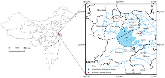
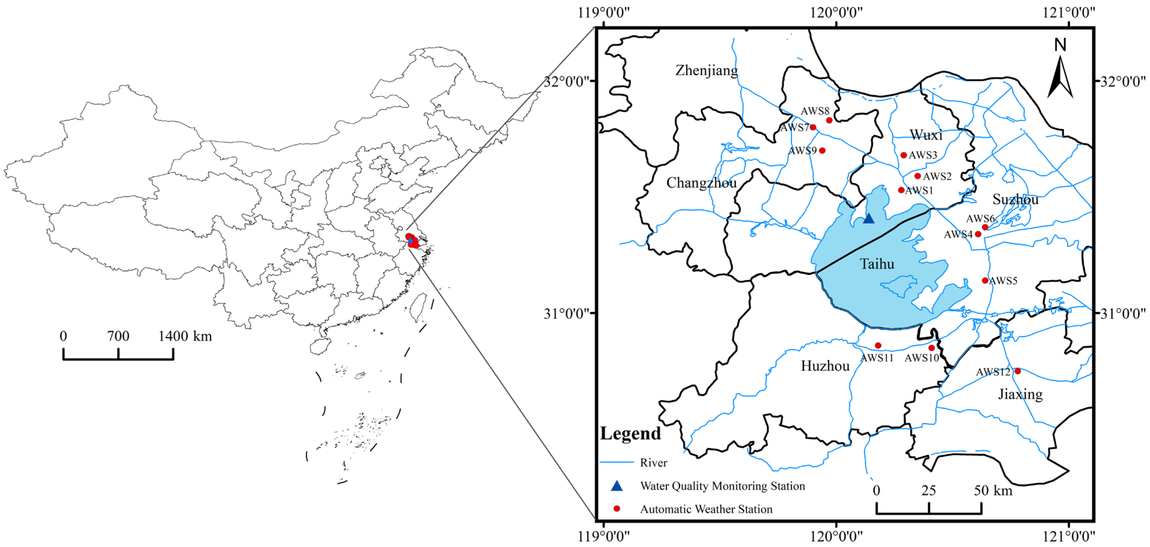
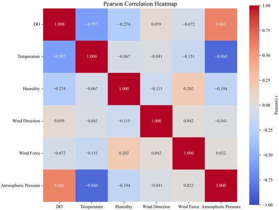
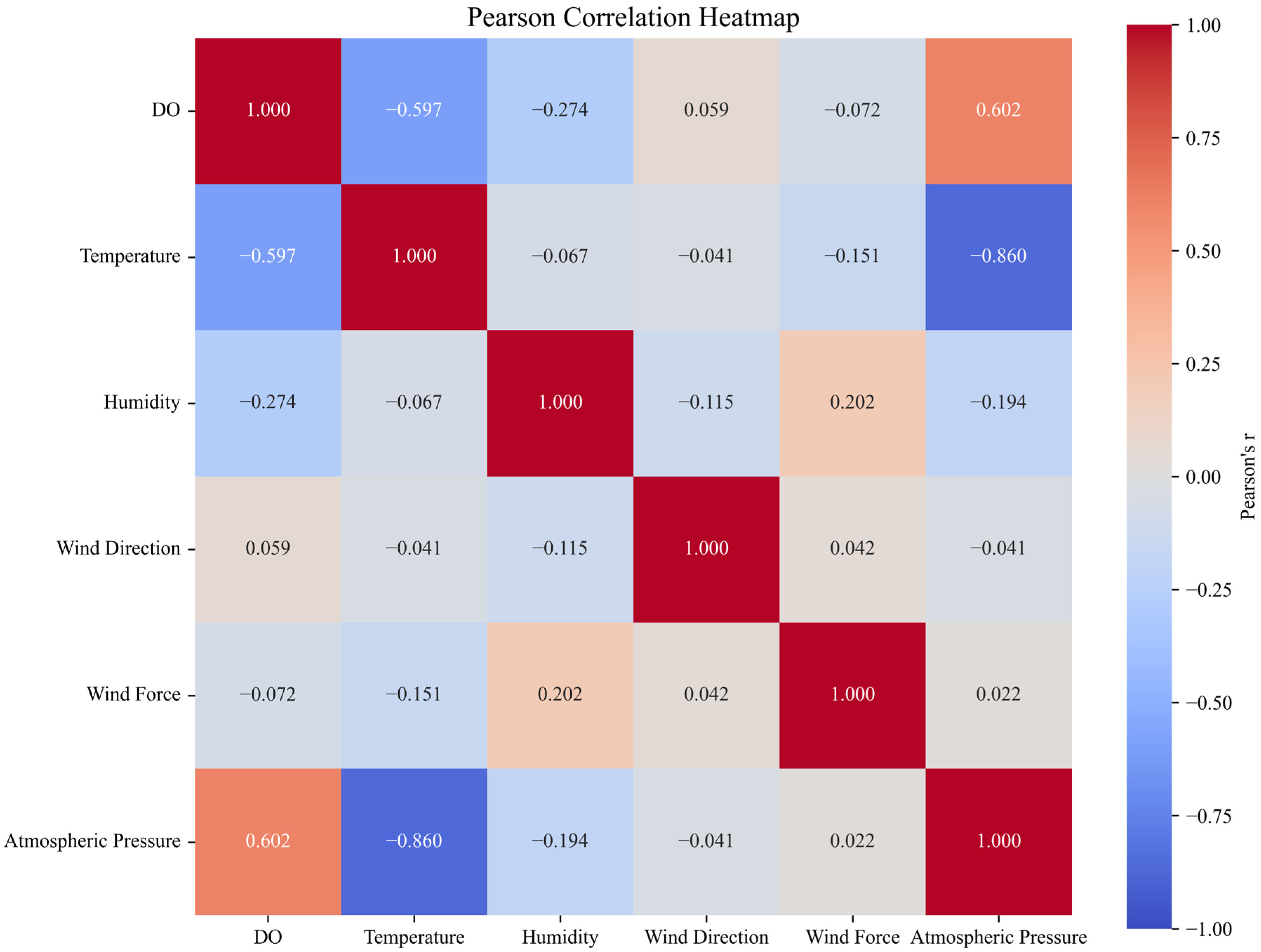
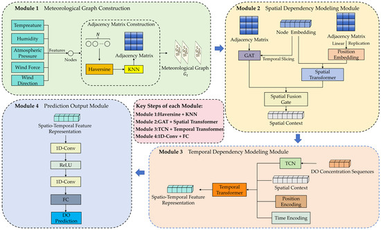
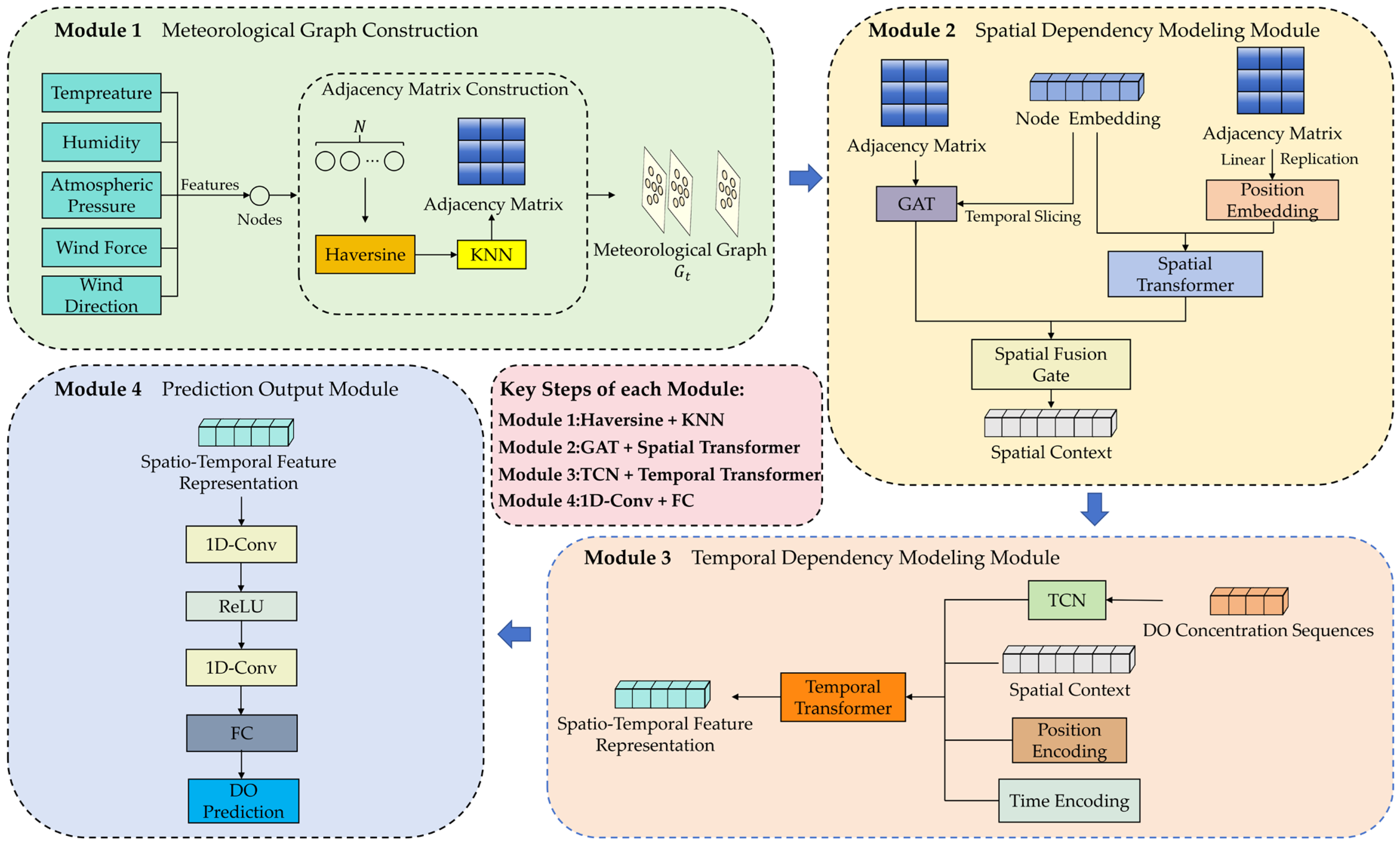
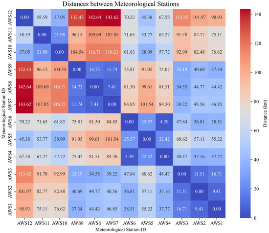
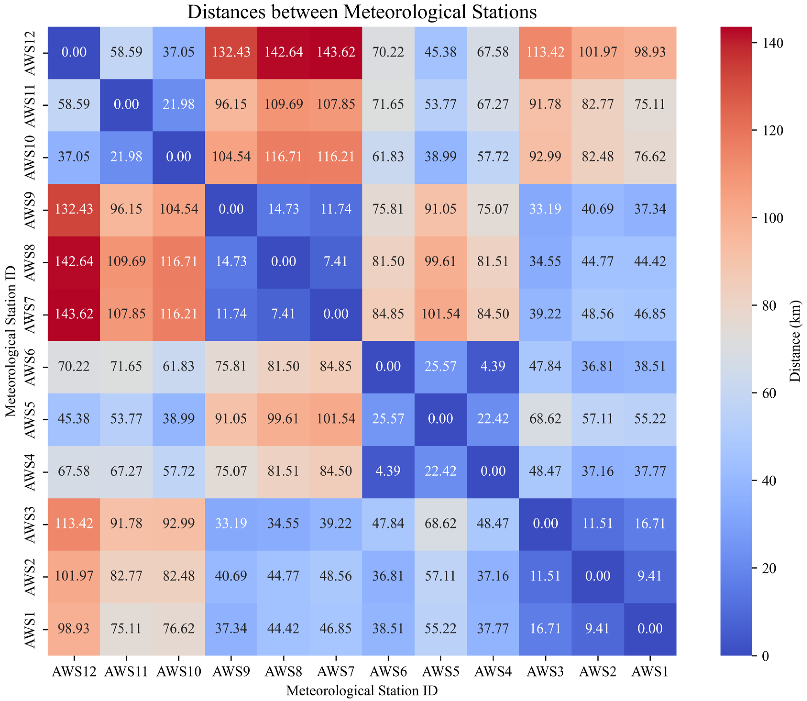




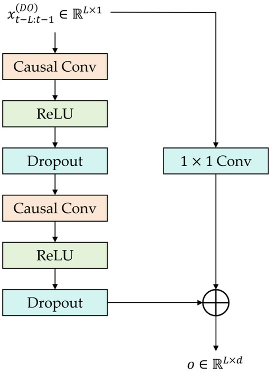
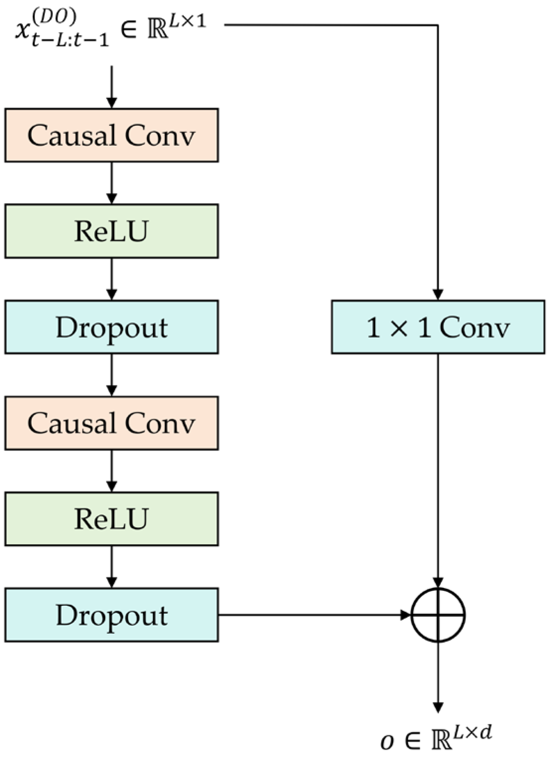
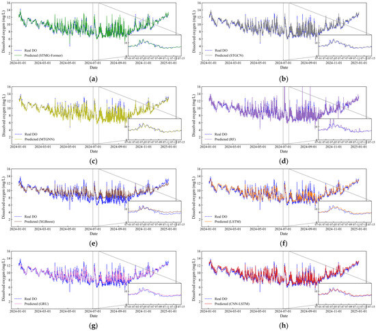
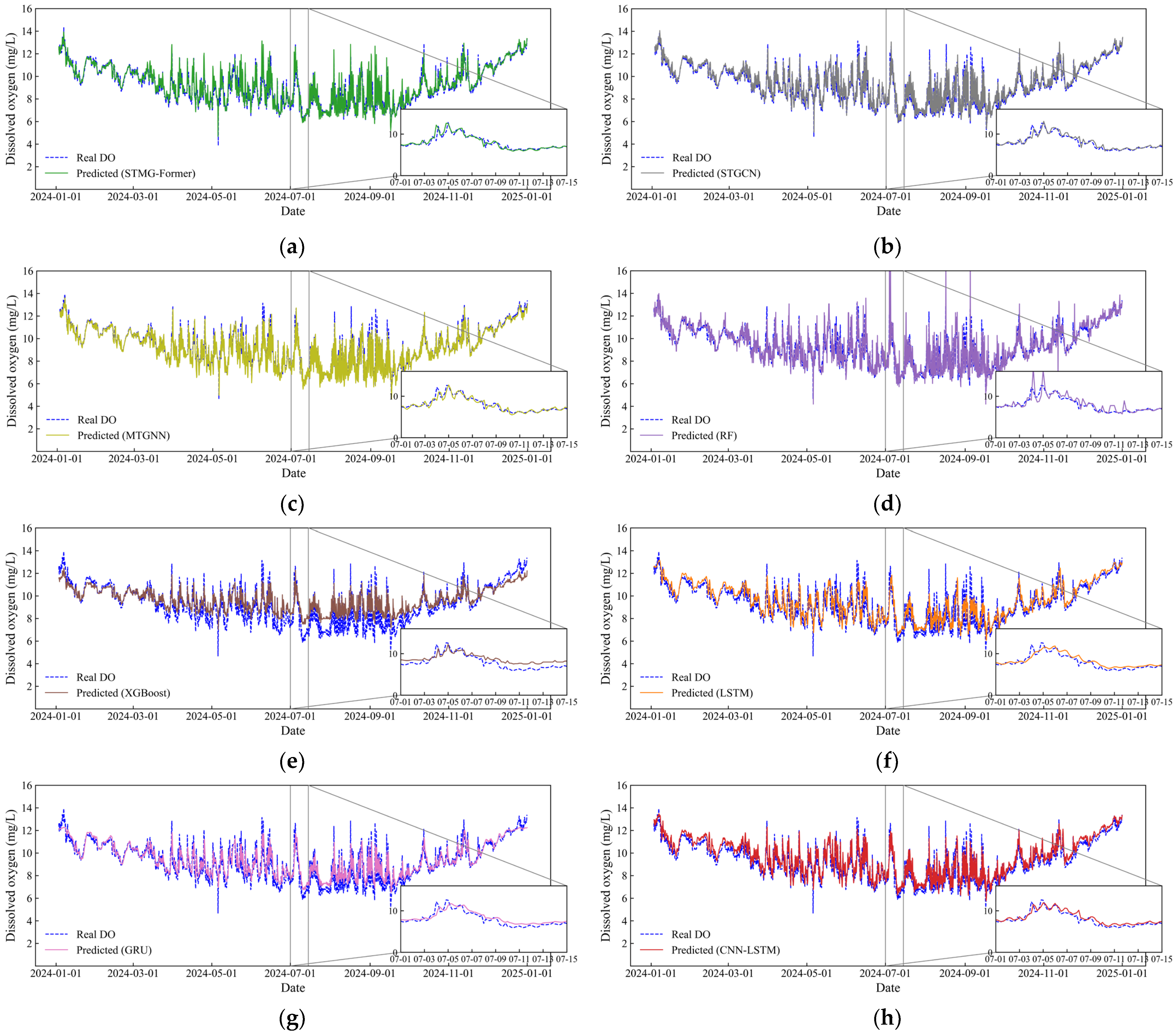
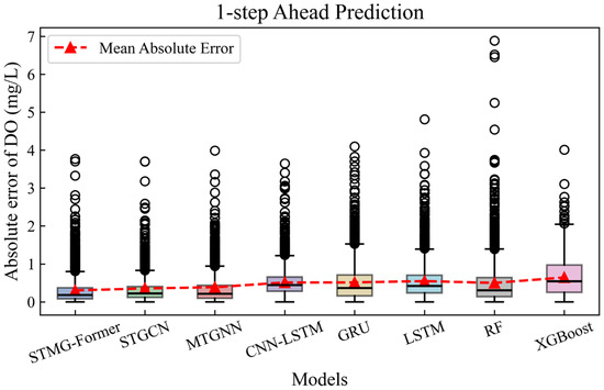
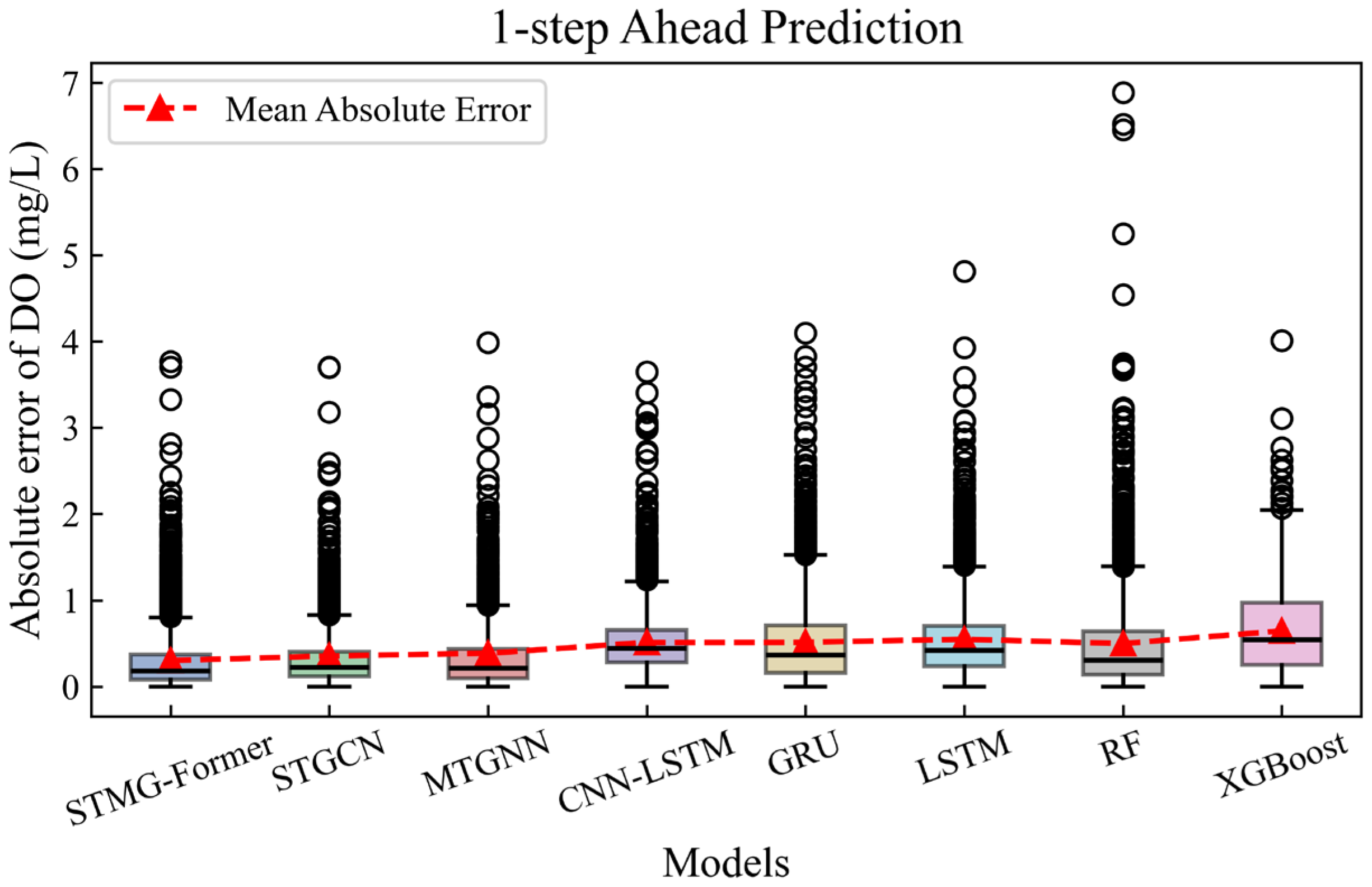
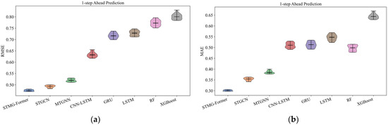
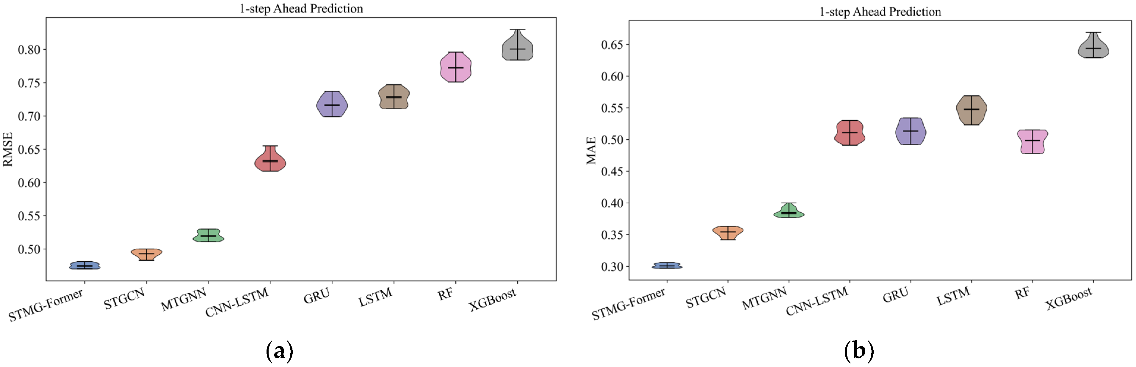
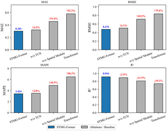
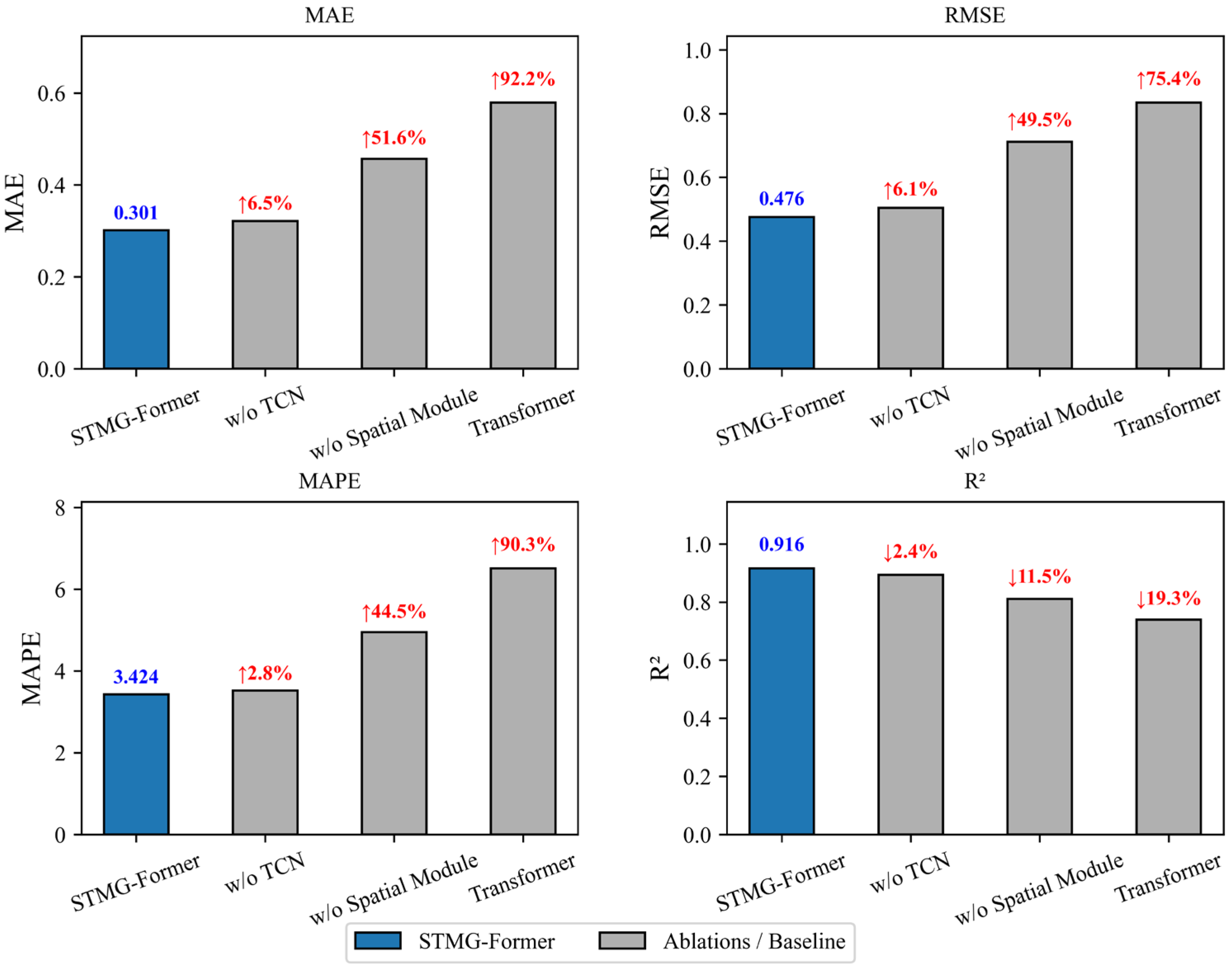
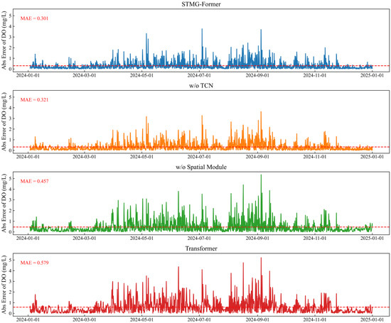
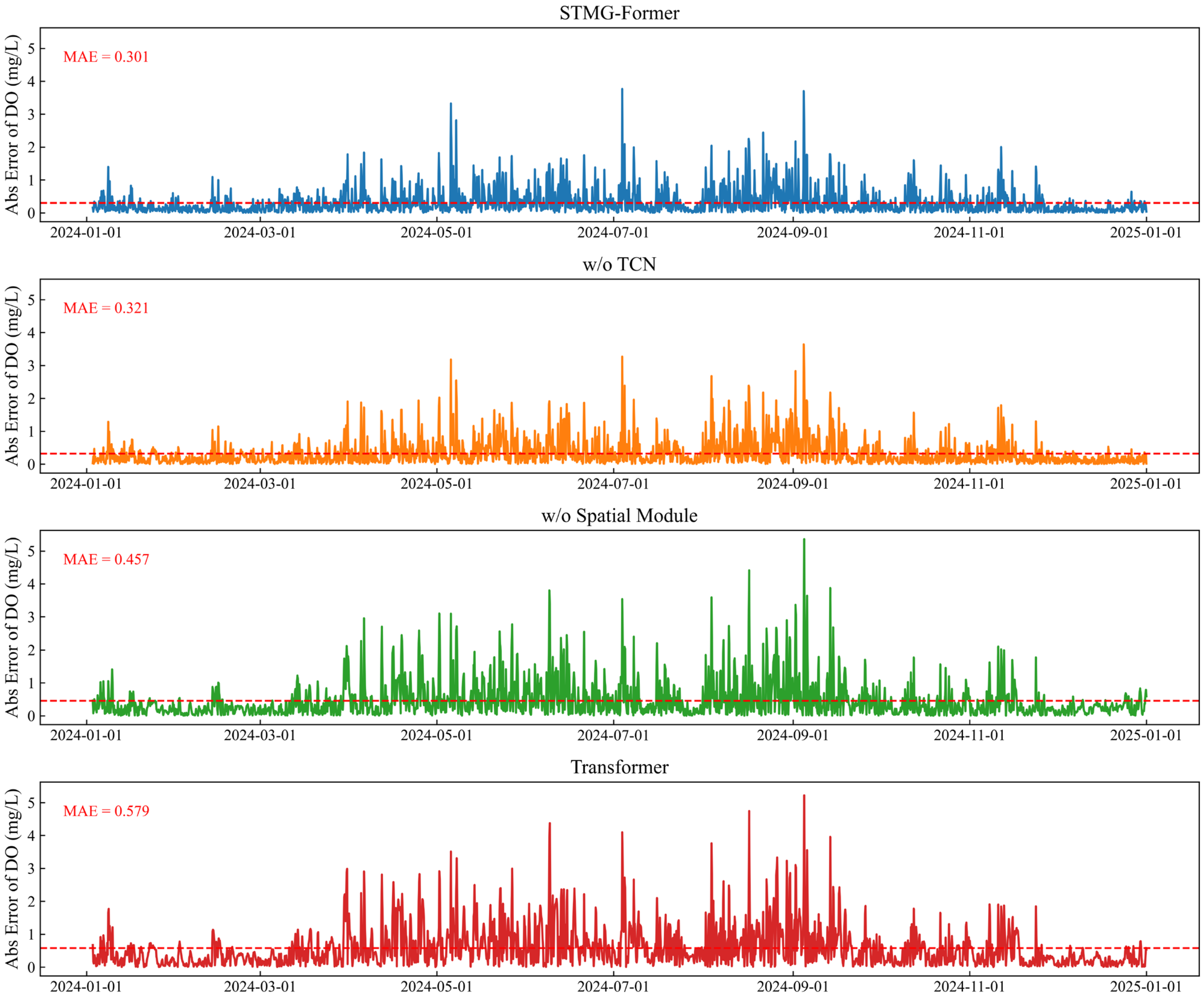
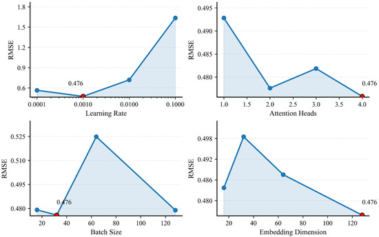
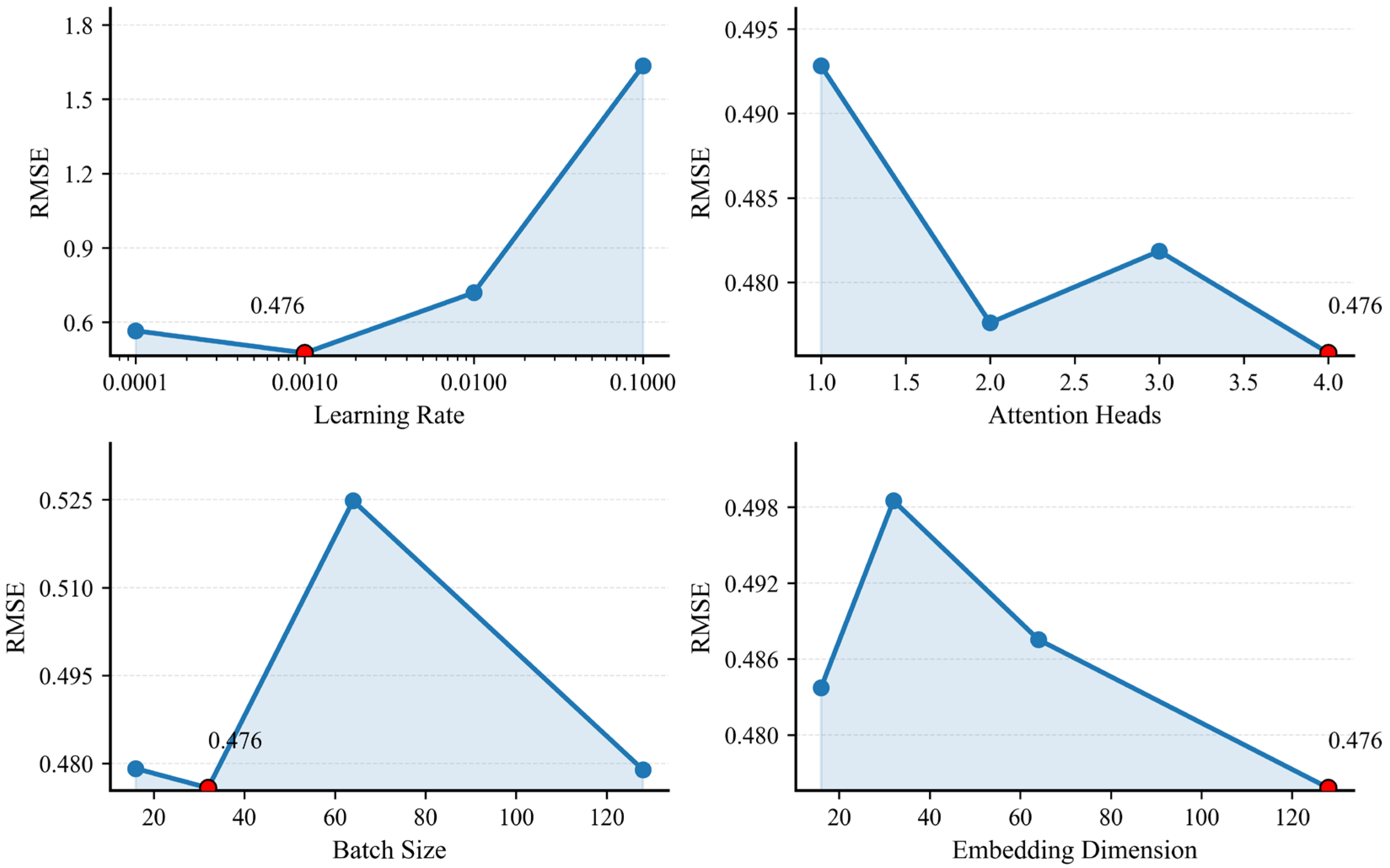
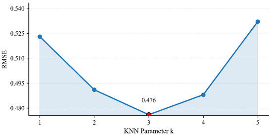
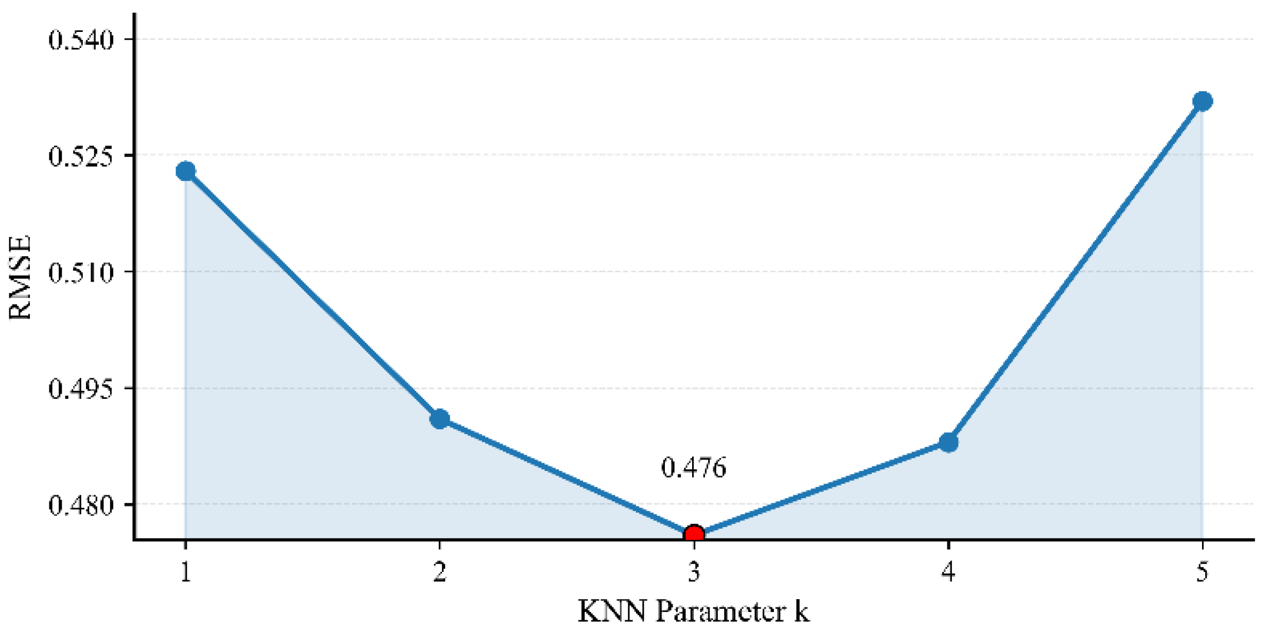
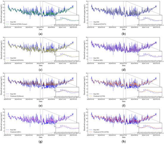
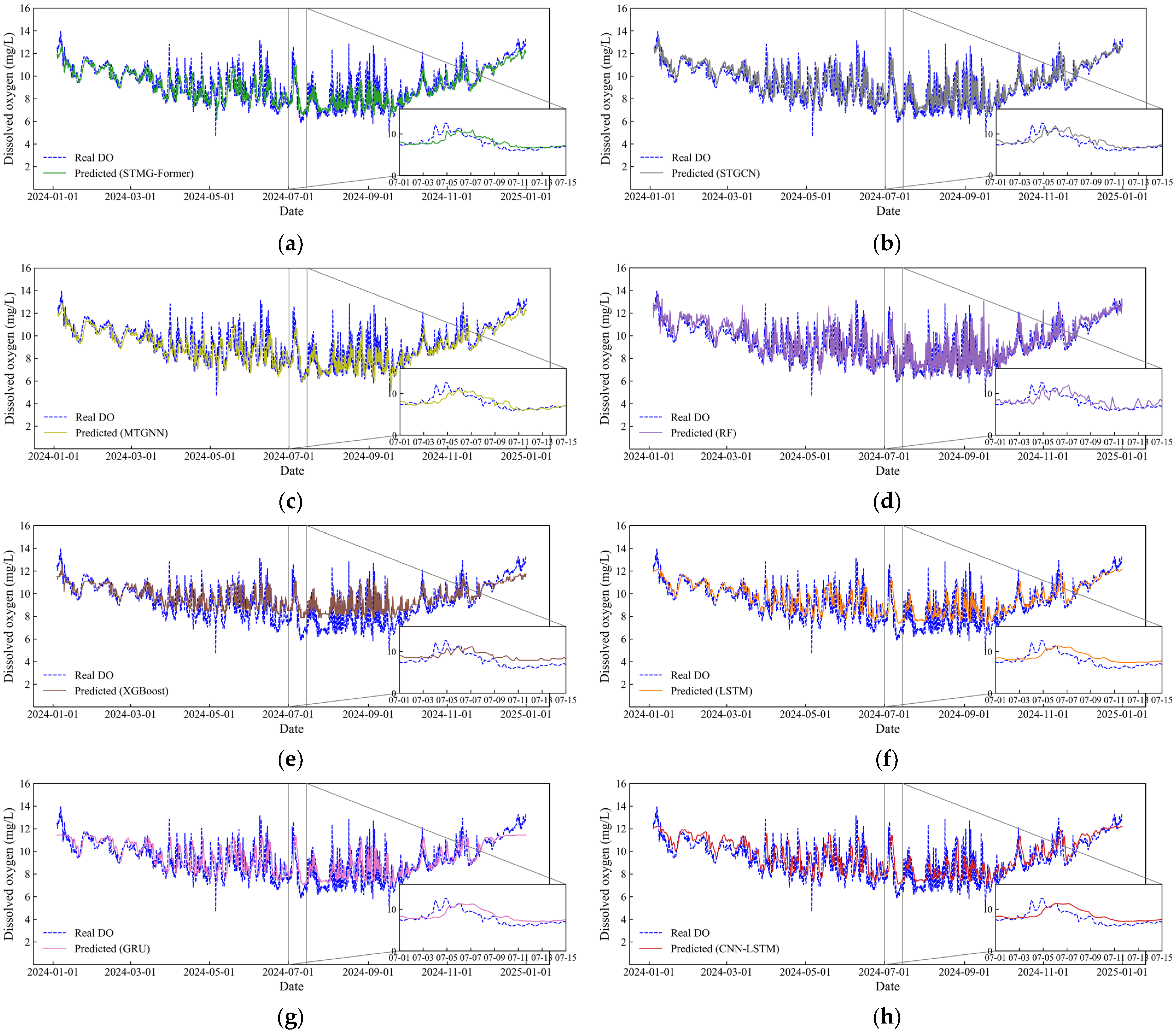
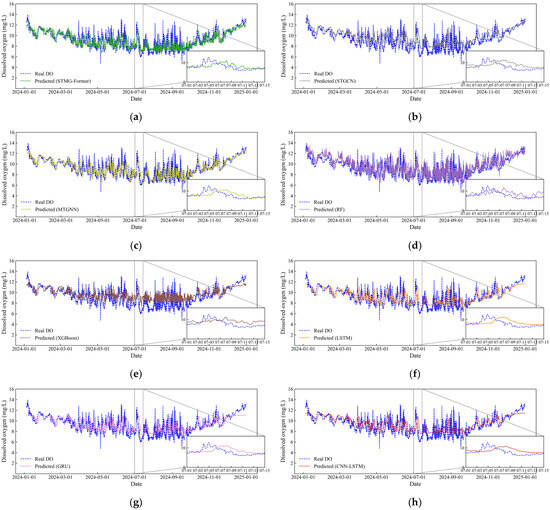
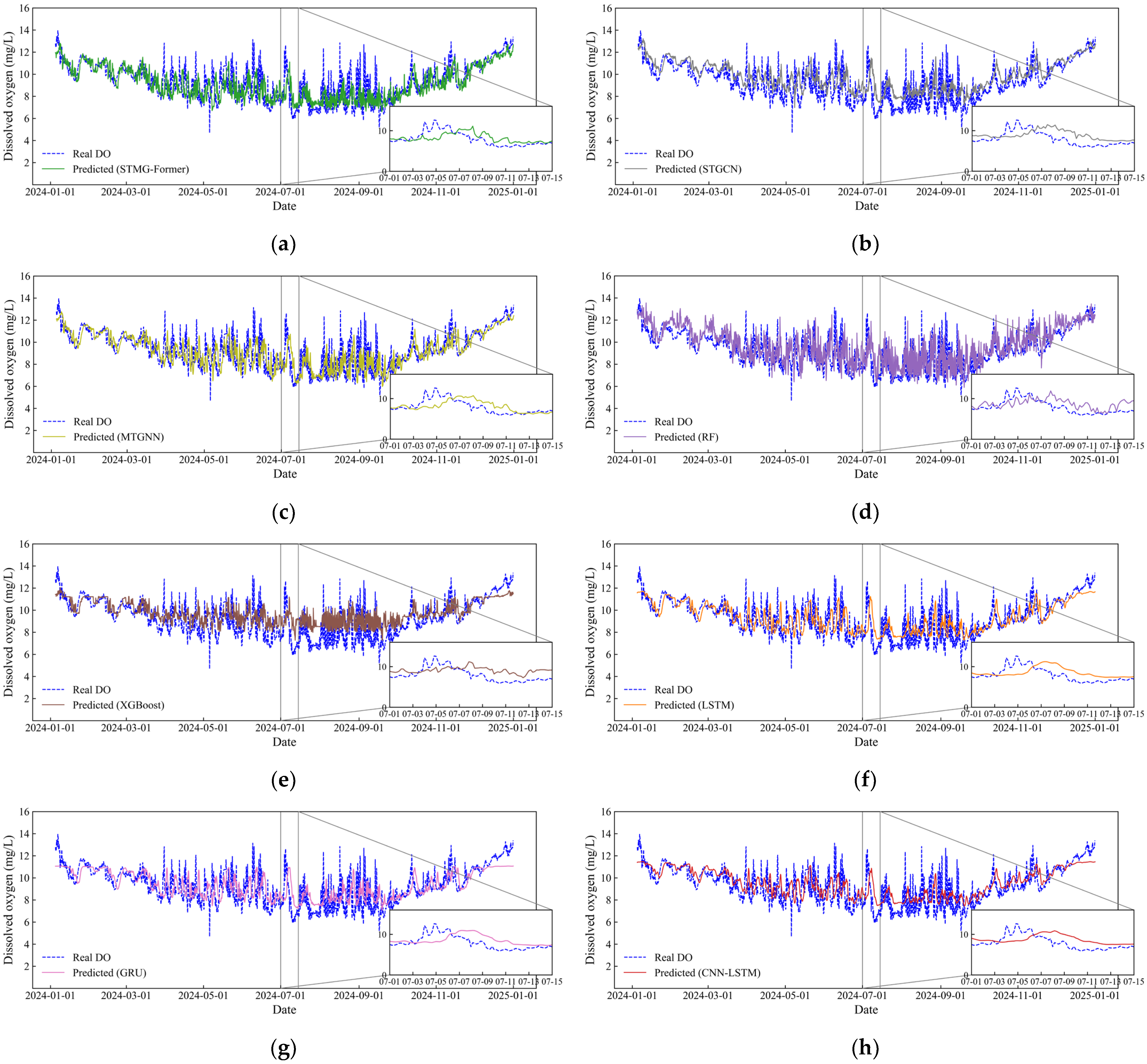
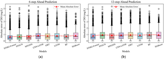
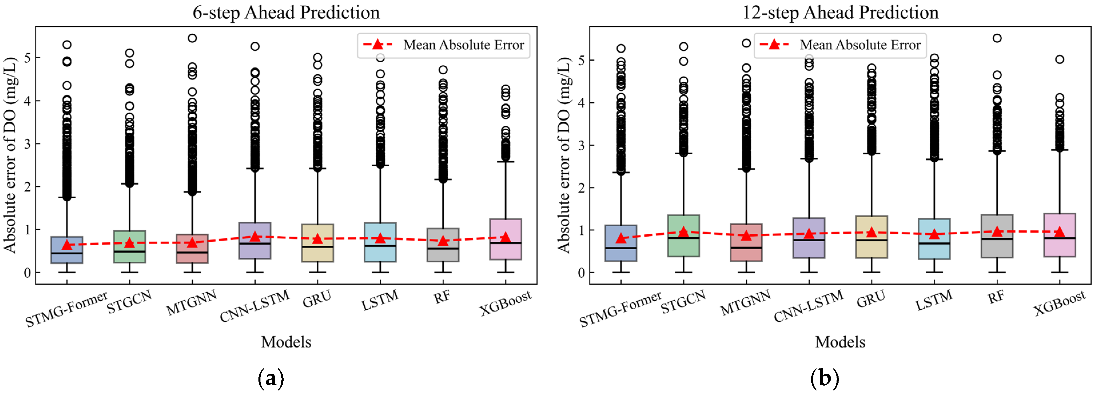
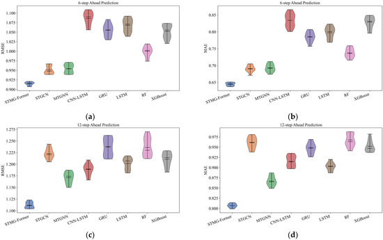
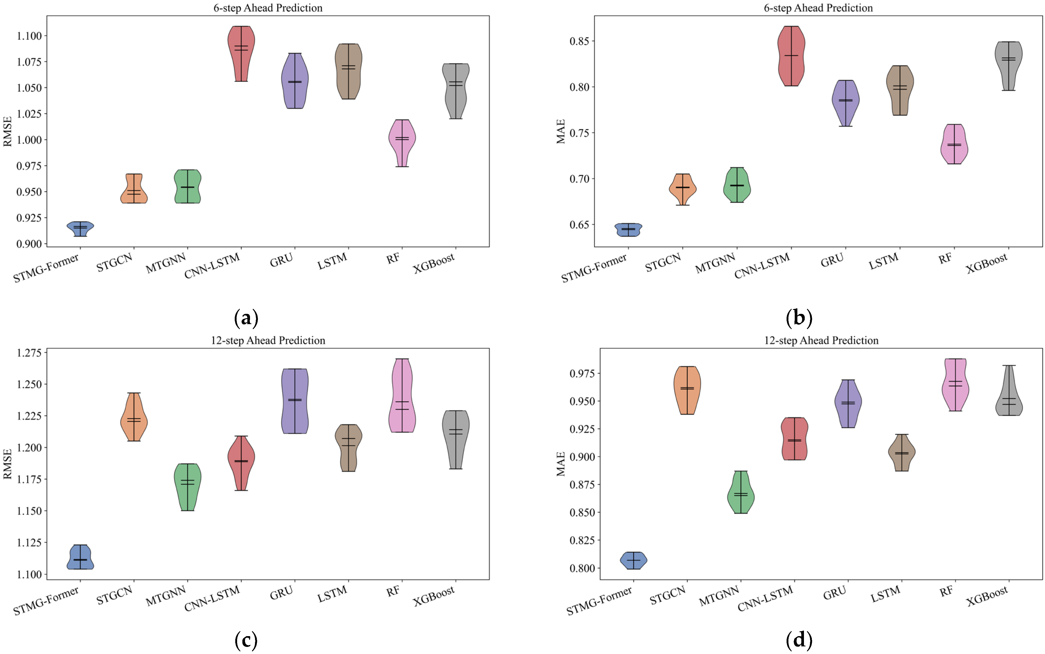

Disclaimer/Publisher’s Note: The statements, opinions and data contained in all publications are solely those of the individual author(s) and contributor(s) and not of MDPI and/or the editor(s). MDPI and/or the editor(s) disclaim responsibility for any injury to people or property resulting from any ideas, methods, instructions or products referred to in the content. |
© 2026 by the authors. Licensee MDPI, Basel, Switzerland. This article is an open access article distributed under the terms and conditions of the Creative Commons Attribution (CC BY) license.