Examining the Super Intense Geomagnetic Storm on 10–11 May, 2024 via Artificial Neural Networks

Abstract

This study investigates the super intense geomagnetic storm of 10–11 May 2024, during which the Dst index reached −412 nT, marking the most severe event of the last two decades. An artificial neural network (ANN) model was developed to estimate the geomagnetic storm indices Dst, Kp, and ap using hourly solar wind parameters (Bz, E, P, N, and V) obtained from the OMNI database. The model successfully reproduced the rapid and nonlinear variations observed during the main phase of the storm. The correlation coefficients (R) between observed and estimated values were 99.5%, 98.8%, and 99.1% for Dst, Kp, and ap, respectively. The corresponding mean square error (RMSE) values were 5.9 nT for Dst, 4.2 for Kp, and 2.1 nT for ap. Despite the extreme geomagnetic disturbance conditions, the ANN architecture maintained high estimative stability and accuracy, particularly during the sharp Dst decrease associated with southward Bz excursions. These results demonstrate that ANN-based approaches can effectively model the nonlinear dynamics of superstorms and provide a reliable complementary tool for forecasting extreme geomagnetic events.

1. Introduction

Extreme changes in space weather conditions can have significant impacts on both the Earth and the technological measuring devices we use. Particularly, solar flares and Coronal Mass Ejections (CMEs) caused by disturbances in the Sun’s magnetic field can release large amounts of particles into space. When these particles reach Earth, they can interact with Earth’s magnetosphere, potentially leading to superstorms. Several well-known superstorms have been studied during solar cycles 22–24, covering the last 30 years. These unique storms have attracted significant interest from the scientific community due to the massive disturbances they generate on Earth [1,2,3,4,5].

A Coronal Mass Ejection (CME) is the eruption of large-scale magnetized plasma from the solar corona into interplanetary space. These plasma structures propagate through the heliosphere with speeds that may exceed 800 km s⁻¹ and can carry strong embedded magnetic fields. When a CME reaches the Earth’s magnetosphere, its geoeffectiveness primarily depends on the orientation of its interplanetary magnetic field (IMF), particularly the southward Bz component. If the CME magnetic field is directed southward, opposite to the Earth’s magnetic field, magnetic reconnection occurs at the dayside magnetopause, leading to enhanced energy transfer into the magnetosphere [6].

A geomagnetic storm (GS) is a temporary (~two days) disturbance of the Earth’s magnetosphere caused by solar wind shock waves and CMEs interacting with the geomagnetic field. During a solar flare, large amounts of energy are released, causing the Sun’s magnetic field lines to change shape. This energetic particle cloud also disrupts the Earth’s magnetosphere–ionosphere system. A GS is observed in three phases:

-

Primary phase;

-

Main phase;

-

Recovery phase [7,8].

During geomagnetic storm conditions, significant variations in solar wind parameters are observed. In many events, changes in solar wind speed, dynamic pressure, and proton density accompany storm development [9]. Therefore, a GS is typically initiated by the arrival of an interplanetary disturbance such as a CME. The occurrence of multiple CMEs may enhance the severity of a geomagnetic storm. After the storm begins, the Bz (nT) component of the magnetic field often turns southward and shows negative values [10,11,12,13]. After Bz reaches its minimum negative value, the Dst (nT) index reaches its minimum value within a few hours. This period is considered the response time of the Dst index to the magnetic field variations. The response time of the Dst index can range from 1 to 3 h for weak storms, 3 to 6 h for moderate storms, and 6 to 9 h for severe GSs [14]. This interval corresponds to the main phase of the GS. In the recovery phase of a GS, the values of the variables that characterize the event dynamics gradually stabilize and return to pre-storm levels. GSs can affect power grids, satellite communications, and other technological systems [15,16,17,18,19,20].

Today, it is widely accepted that the energy distributed into the Earth’s atmosphere during a superstorm is extremely large and causes significant changes in the ionosphere. This has been confirmed by many scientific studies [21,22,23,24,25]. When a superstorm occurs, ionospheric disturbances and aurorae extend to significantly lower latitudes than normal. This research examines how this latitudinal expansion affects GNSS signals and degrades positioning accuracy. Several scientific studies on this topic have been conducted. Early studies such as Freeman et al. [26] demonstrated the potential of neural networks for forecasting magnetospheric parameters, while Kugblenu et al. [27] applied ANN methods to predict the storm-time Dst index. Subsequent studies developed ANN-based operational models for the prediction of Dst and Kp from solar wind parameters [28]. More recently, improved neural network architectures and hybrid approaches have been used to enhance the prediction of geomagnetic activity indices, including Dst, Kp, SYM-H, and ap [29,30,31,32]. Astafyeva et al. [33] analyzed GPS performance during four GSs with varying intensities using data from globally distributed GPS stations. Luo et al. [34] investigated the Global Positioning System–Precise Point Positioning (GPS PPP) accuracy at 500 stations distributed homogeneously on the Earth’s surface under different GS conditions. Liu et al. [35], Zakharenkova et al. [36], Kong et al. [37], Senturk [38], Feng et al. [39], Eroglu [40], Nie et al. [41], and Sierra-Porta et al. [42] have studied the effects of superstorms on the ionosphere using GNSS observations and predicted GSs using machine learning techniques. He et al. [43] evaluated the quality of BeiDou Navigation Satellite System (BDS) carrier-phase observation signals during the GS of 12 May 2021. Luo et al. [44] and Wang et al. [45] assessed the performance of GNSS Precise Point Positioning under strong GS conditions, noting that GSs reduce positioning performance. Atabati et al. [46], Tahir et al. [47], and Sun et al. [48] have tried to determine the relationship between GS severity and the total electron content (TEC) using data from multiple sensors such as plasma density, Formosat-7/Cosmic-2 (F7/C2), radio occultation profiles, and solar wind parameters.

Previous studies have attempted to identify the effects of low, moderate, and severe storms on Earth using different parameters. The most recent superstorm, referred to as the 2024 Mother’s Day super GS, occurred on 10–11 May 2024, and is recorded as the largest GS observed on Earth in the last 20 years. During this storm, Karan et al. [49] observed that the Equatorial Ionization Anomaly (EIA) merged with the aurora in the American longitude, resulting in the disappearance of the mid-latitude ionosphere. Evans et al. [50] reported that the thermospheric temperature difference between the equator and the poles exceeded 126 °C. Guo et al. [4] revealed ionospheric differences between the east–west regions of East Asia during the superstorm of 11 May 2024.

These scientific studies have partially considered GS indices such as F10.7 solar radio flux, proton density, and Dst. The F10.7 solar radio flux (measured at a wavelength of 10.7 cm, 2800 MHz) is widely used as a proxy for solar activity and EUV (Extreme Ultraviolet) emissions. Since each superstorm, including the ones that will occur in the future, could lead to massive changes on Earth, it is necessary to characterize their specific features in detail. Although the May 2024 superstorm has already been examined in recent studies, including AI-based investigations, the contribution of the present study is different in scope. Rather than addressing the full chain of solar active region evolution, flare forecasting, CME propagation, and storm alerting, this work focuses specifically on the event-based ANN modeling of three standard geomagnetic storm indices, namely Dst, Kp, and ap, using hourly OMNI solar wind parameters during the 10–11 May 2024 superstorm. In this sense, the study provides a focused assessment of how a unified ANN framework represents the temporal behavior of these indices during an extreme geomagnetic event. While the existing literature has extensively examined the influence of solar wind and solar-origin indices on geomagnetic storm activity, studies that simultaneously integrate magnetic field parameters, plasma density variations, and GNSS station observations to model the dynamics of extremely intense storms remain limited. In this research, an artificial neural network model capable of capturing the nonlinear and abrupt variations observed during high-intensity events (Dst = −412 nT) is employed. The results indicate that the proposed approach offers a complementary alternative to traditional linear methods and has the potential to contribute to more consistent predictions of the impacts of future extreme geomagnetic storms.

In this study, the super geomagnetic storm that occurred on 10–11 May 2024 has been modeled and analyzed using artificial neural networks (ANNs). The architecture and parameters of the artificial neural network (ANN) employed in this study are discussed in detail in Section 3. The Dst index of the superstorm on 11 May 2024 was −412 nT. The ANN model uses solar wind parameters (SWPs) as the input and estimates the indices as the output. The estimation of the indices using the ANN model (ANNm) shows significant consistency. The estimation results were evaluated using mean square error (MSE) (Table 1).

Table 1. Correlation ratio (R) and mean square error (MSE) values of ANN models.

Storm	Parameter	Correlation Ratio (R)	Mean Square Error (MSE) (nT)
11 May 2024 Dst (−412 nT)	Dst	99.5%	5.9274
	Kp	98.8%	4.2499
	ap	99.1%	2.0859

This study examines the features of the superstorm that occurred on 10–11 May 2024, recorded as the largest geomagnetic storm observed in the last 20 years. During the superstorm, geomagnetic storm indices, namely Dst, Kp and ap, were estimated by using an ANN model.

2. Data Source

The study utilized hourly data from the OMNIWeb (https://omniweb.gsfc.nasa.gov/form/dx1.html, accessed on 12 December 2025) database and focused on the May 2024 superstorm. This superstorm is part of a series of exceptionally powerful solar storms, including intense solar flares and geomagnetic disturbances, which have persisted since 10 May 2024, during Solar Cycle 25 [51]. The GS has been recorded as the most powerful storm to affect Earth since 20 November 2003, and has caused auroras to be visible at much lower latitudes than usual in both the northern and southern hemispheres [52]. The solar wind parameters, including the interplanetary magnetic field southward component (Bz), solar wind electric field (E), dynamic pressure (P), plasma density (N), and solar wind speed (V), were obtained from the OMNI database with a temporal resolution of [1 h].

The geomagnetic activity during the storm was characterized using the Dst, Kp, and ap indices, which were obtained from the World Data Center for Geomagnetism. These indices were used as target outputs for the artificial neural network model.

3. Geomagnetic Storm Indices

The variations in the Dst, Kp, and ap indices between 1 and 31 May 2024 are presented in Figure 1.

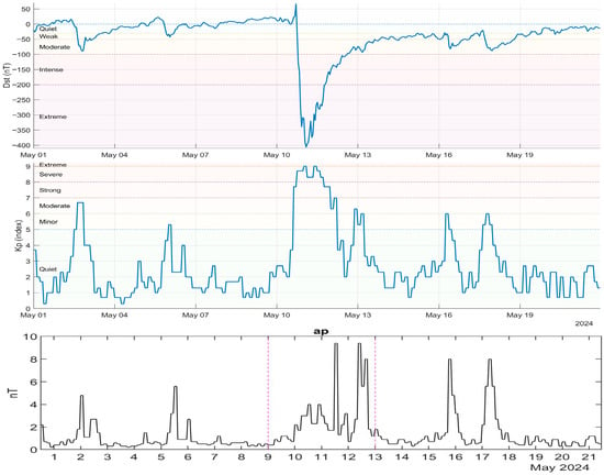
Figure 1. Dst, Kp and ap indices for the superstorm on 11 May 2024.

Figure 1 and Figure 2 show the values of Dst, Kp, and ap indices. The threshold values for these indices were adopted from [14]. In Figure 1, Figure 2 and Figure 3 the data obtained from OMNIWeb (https://omniweb.gsfc.nasa.gov/form/dx1.html, accessed on 12 December 2025) have been illustrated by in house software.

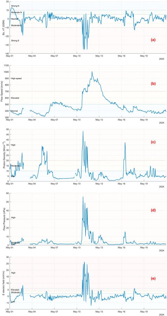
Figure 2. (a) The Bz (nT), (b) the v (km/h), (c) the N (cm⁻³), (d) the P (nPa), and (e) the E (mV/m) for May 2024 superstorm.

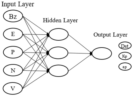
Figure 3. The network structure.

Figure 1 presents the temporal variations in the Dst, Kp and ap indices between 1 and 31 May 2024. Two geomagnetic disturbances are evident during this interval. The first storm occurred on 2 May, when Dst decreased to −89 nT, indicating a moderate geomagnetic event. The second and most intense disturbance developed on 10–11 May, characterized by a sudden positive excursion in Dst followed by a rapid transition into an extreme storm. The minimum Dst value reached −412 nT, classifying the event as an extreme geomagnetic storm. The Kp index exhibited enhanced activity concurrent with both disturbances and reached its maximum value (Kp = 9) during the peak of the 11 May event. The ap index followed a consistent pattern with Kp, confirming the strong geomagnetic response.

The variations in the Bz_GSM, flow speed (v), proton density (N), flow pressure (P), and electric field (E) parameters between 1 and 31 May 2024 are shown in Figure 2.

Figure 2 summarizes the interplanetary drivers of the 10–11 May storm. A southward turning of the IMF Bz component preceded the main phase, with a pronounced negative excursion prior to the Dst minimum. Solar wind conditions were relatively quiet before 10 May; however, a clear acceleration phase followed, with wind speed exceeding 1000 km/h during the storm evolution. Proton density and dynamic pressure exhibited sharp enhancements associated with successive CME arrivals, indicating strong solar wind–magnetosphere coupling. The most significant pressure pulse coincided with the storm’s main phase, supporting the interpretation that the sudden commencement and subsequent intensification were driven by enhanced dynamic pressure and sustained southward Bz conditions. The main phase extended from late 10 May to early 11 May, culminating in the extreme Dst minimum.

Figure 1 and Figure 2 show the values of Bz_GSM, flow speed (v), proton density (N), flow pressure (P) and electric field (E) indices. The threshold values for these indices were adopted from [53].

4. Artificial Neural Network (ANN) Theory

The aim of this ANN application is not to provide a general end-to-end space weather forecasting system, but to evaluate whether the temporal variations in Dst, Kp, and ap during the May 2024 superstorm can be represented consistently from hourly solar wind inputs within a single event-oriented framework. The neural network is a learning and modeling structure that is an imitation of the human brain. This structure processes data images, makes estimations, translates, creates pattern relationships, and confronts humans in many other areas. The neural network consists of layers connected by neurons. Figure 3 shows the neural network frame.

Data received from the input layer is processed in intermediate layers and presented as a product from the output layer. Inter-layer process management is organized by neurons. A sufficient number of neurons should be used to prevent memorization or failure to learn [54,55]. The learning ability of the neural network is directly related to the number of neurons. Raw data received from the input layer is normalized and standardized if necessary; missing data is discarded or completed. In this study, the authors use the raw data, without normalization and completion. Neural network training is a set of procedures. In this sense, the network training–teaching procedure has certain stages to teach the network to perform a certain task. First of all, the layers and tasks are determined. Then, according to these, layer numbers, number of neurons, activation sign, and iteration preference are constructed. In the next stage, the labeled data is taken from the input layer. Training, testing, and validation partitioning are performed for the dataset. Then, the neural network determines the weights and biases of the inputs. The model of the work uses Equation (1) as the stimulation (activation) function:

$$y_{ij}={\displaystyle \sum _{k=1}^n}{w}_{kj}{x}_{ik}+b_j$$

(1)

where w denotes the synaptic weight, x the input, y the output, and b represents the bias term. The bias acts as an intercept parameter in the linear combination of inputs, shifting the decision boundary and controlling the activation threshold of the neuron. In this study, the input vector x consists of hourly solar wind parameters, including the southward component of the interplanetary magnetic field (Bz), the interplanetary electric field (E), solar wind dynamic pressure (P), proton density (N), and solar wind speed (V). The interplanetary electric field (E) was computed using the convective electric field formulation, defined as E = −v × B, where v represents the solar wind velocity vector and B denotes the interplanetary magnetic field (IMF). Here, P refers to the solar wind dynamic pressure, N to the proton density, and V to the solar wind speed. These parameters are used as inputs to the ANN model to estimate the geomagnetic indices Dst, Kp, and ap. Accordingly, $x_{ik}$ represents the $k^{th}$ solar wind parameter (Bz, E, P, N, or V) at time i, where $w_{ik}$ denotes the corresponding synaptic weight. Synaptic weights in artificial neural networks (ANNs) are numerical parameters assigned to the connections between artificial neurons (nodes) that determine the strength and polarity of the signal transmitted between them. These weights are iteratively adjusted during training to minimize the loss function and optimize the model performance. The sigmoid transfer function Equation (2) is

$$f\left(y\right)={\displaystyle \frac{1}{1+e^{-y}}}$$

(2)

where f is the logistic function. The sigmoid activation function was selected due to its smooth, nonlinear, and differentiable structure, which makes it suitable for gradient-based optimization algorithms such as backpropagation. The logistic function maps input values into the interval (0, 1), enabling the network to model nonlinear relationships between solar wind parameters and geomagnetic indices. Sigmoid functions have been widely used in geomagnetic index estimation and space weather modeling studies [55,56,57]. Alternative activation functions such as hyperbolic tangent (tanh), Rectified Linear Unit (ReLU), and its variants (Leaky ReLU, ELU) could also be employed. The tanh function maps outputs into the interval (−1, 1) and often provides faster convergence due to its zero-centered property. ReLU-based functions are computationally efficient and mitigate vanishing gradient problems in deeper architectures. However, since the present model employs a relatively shallow feed-forward ANN and aims to capture bounded nonlinear relationships in hourly solar wind parameters, the sigmoid function was considered sufficient and computationally stable for this application.

Forward propagation uses the network to obtain the outputs as an estimate. This method calculates the loss that indicates the difference between the estimated output and the real output data. Backpropagation is used to calculate the gradients of the loss related to the network parameters using the chain rule [58]. It learns by going back at each step and learning from the errors. It reduces the weights and biases by using an optimization algorithm. Both approaches are iteration-based. The study uses the parameters of the interplanetary plasma, i.e., the solar wind, as input. The input data is directed to the hidden layer with the activation signal [54,59,60]. The hidden segment or segments (multiple hidden segments can be established) come after the input segment. They are hidden because the training tools may not have been noticed directly. As mentioned before, training is managed by neurons. A processed dataset is created with the weights loaded on the inputs and their biases. The authors use feedback iteration in this study. Each iteration is a step for feedback. The model learns at each step. This is the training process for the model. Iteration continues until the results reach perfection. The correct output for the data coming from the input node is unique. It is in the form of a loop. The accuracy of the estimation is checked. Nodes strengthen the connections that are closest to the correct estimations. In other words, they increase the weights of these connections. They decrease the weights of the ones that are far away. This procedure runs continuously. Finally, the error of each step is minimized and the network is learned. The network gains a nonlinear perspective with the activation signal. The most commonly used ones are the logistic function (results between 0 and 1) and tanh (results between −1 and 1). The bias in Equation (1) is a complementary term that helps to set the activation threshold of a neuron. The final part of the neural network is the output layer. It is the layer where the results of the model are received. The products of this work are the geomagnetic indices Dst (nT), Kp, and ap (nT). The performance of the neural network model is determined by the loss function and its auxiliary elements. The loss function uses the correlation coefficient (R) and the mean squared error (MSE) rate to evaluate the consistency and accuracy of the model. The R rate is

$$R={\displaystyle \frac{Cov(x,y)}{\sqrt{Var\left[x\right]Var\left[y\right]}}}$$

(3)

where cov(x,y) is the covariance of x and y; var[x] and [y] are the variances of x and y, respectively. The R score bears the strong effect of the association between the two data. The MSE (nT) score employed for sensing deviations is

$$MSE={\displaystyle \frac{1}{n}}\sum {\left(y_{observed}-y_{estimated}\right)}^2$$

(4)

The neural network prototypes employ a 21-day (504 h) dataset for the modeling of the Dst, Kp, and ap zonal geomagnetic indices. In all our education models, 75% of the data for training, 20% of the data for validation, and 5% of the data for testing are used. This partitioning strategy was selected to ensure sufficient data for model training while preserving independent datasets for generalization assessment. Similar data-splitting ratios (70–80% for training and the remaining portion for validation and testing) are commonly used in ANN-based space weather estimation studies [55,59]. The relatively larger test proportion (5%) was chosen to provide a robust evaluation of the model’s estimative capability during extreme geomagnetic storm intervals, where generalization performance is critical. Figure 4 shows R correlation constants for the Dst index modeling. The procedure used for the Dst index modeling accomplishes a 99.5% correlation rate and 5.93 nT MSE score after 187 epochs with the aid of thirty neurons.

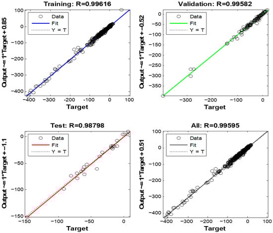
Figure 4. Correlation scores for the Dst modeling.

Figure 5 exhibits the MSE rate and average R correlation score.

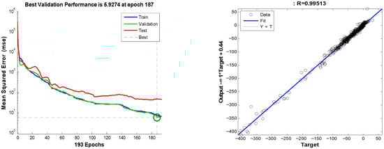
Figure 5. MSE rate and the model average correlation score for the Dst modeling.

Figure 6a,b displays the appearances of the Dst zonal geomagnetic index, the estimated Dst, and its error, respectively. The Dst average value is −49.56 nT, the estimated Dst (Dst est) is −49.40 nT, and the error is 0.66 (%).

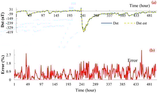
Figure 6. (a) The appearances of the Dst (nT) and estimated Dst (nT) zonal index. (b) The error score oscillation between the Dst (nT) and estimated Dst (nT) zonal index.

Figure 4, Figure 5 and Figure 6 illustrate the performance of the ANN model in estimating the Dst index during the May 2024 superstorm. The high correlation values obtained for the training, validation, and test datasets indicate that the model successfully captures the dominant nonlinear relationship between solar wind parameters and the Dst response. As shown in Figure 6a, the estimated Dst closely follows the observed index throughout the storm phases, including the sudden commencement, main phase, and recovery phase. Minor deviations are primarily observed near the peak negative excursion of Dst, which is expected due to the abrupt energy injection and highly dynamic magnetospheric conditions during the storm maximum. Nevertheless, the error magnitudes remain small, confirming the robustness of the model under extreme geomagnetic conditions.

Figure 7 shows R correlation constants for the Kp index modeling.

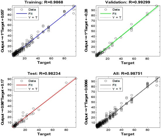
Figure 7. Correlation scores for the Kp modeling.

The process used for the Kp index modeling achieves a 98.75% correlation rate and 4.25 MSE score after 100 epochs with the aid of twenty-five neurons. Figure 8 exhibits the MSE rate and average R correlation score.

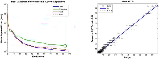
Figure 8. MSE rate and the model average correlation score for the Kp modeling.

Figure 9a,b exhibits the presence of the Kp zonal geomagnetic index, the estimated Kp, and its error, respectively. The Kp average value is 26.95, the estimated Kp (Kp est) is 26.92, and the error is 0.40 (%).

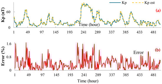
Figure 9. (a) The appearances of the Kp and estimated Kp zonal index. (b) The error score oscillation between the Kp and estimated Kp zonal index.

The modeling results for the Kp index, presented in Figure 7, Figure 8 and Figure 9, demonstrate that the ANN approach is capable of reproducing the temporal variability of Kp with high accuracy. The estimated Kp values show strong agreement with the observed index, particularly during periods of elevated geomagnetic activity. Slight discrepancies appear during rapid Kp transitions, reflecting the quasi-logarithmic nature of the Kp scale and its inherent discretization. Despite these challenges, the low error levels and high correlation coefficients indicate that the model effectively learns the underlying storm-time dynamics governing Kp variations.

Figure 10 shows R correlation constants for the ap zonal geomagnetic index modeling.

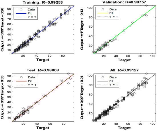
Figure 10. Correlation scores for the ap modeling.

The process used for the ap index modeling gains a 99.13% correlation rate and 2.09 nT MSE score after 55 epochs with the aid of twenty neurons. Figure 11 exhibits the MSE rate and average R correlation score.

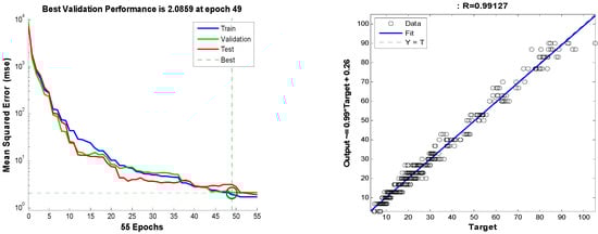
Figure 11. MSE rate and the model average correlation score for the ap modeling.

Figure 12a,b exhibits the presence of the ap zonal geomagnetic index, the estimated ap, and its error, respectively. The ap average value is 13.91 nT, the estimated ap (ap est) is 13.93 nT, and the error is 0.35 (%).

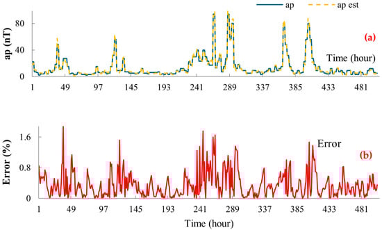
Figure 12. (a) The appearances of the ap (nT) and estimated ap (nT) zonal index. (b) The error score oscillation between the ap (nT) and estimated ap (nT) zonal index.

Figure 10, Figure 11 and Figure 12 present the estimation results for the ap index, which is linearly derived from Kp. The ANN model exhibits excellent performance in capturing both the magnitude and temporal evolution of ap during the storm interval. Compared to Kp, the ap index shows smoother behavior, which facilitates more stable learning by the ANN and results in lower error levels. The close correspondence between observed and estimated ap values across all storm phases highlights the suitability of the proposed ANN configuration for modeling continuous geomagnetic indices.

Previous studies have employed different ANN architectures and training strategies for geomagnetic index estimation (Table 2). For example, Lundstedt et al. [57] utilized a feed-forward multilayer perceptron (MLP) with a sigmoid activation function trained via standard backpropagation to forecast the Dst index using solar wind parameters as inputs. Reference [57] applied a similar MLP structure but incorporated time-lagged solar wind parameters to improve short-term forecasting capability. More recent studies have adopted alternative network configurations. Some researchers implemented recurrent neural networks (RNNs) to account for temporal dependencies in geomagnetic storm evolution, while others applied Long Short-Term Memory (LSTM) networks to better capture nonlinear and delayed magnetospheric responses to solar wind forcing. In addition, activation functions such as hyperbolic tangent (tanh) and Rectified Linear Unit (ReLU) have been used instead of the logistic sigmoid function defined in Equation (2), primarily to mitigate gradient saturation and accelerate convergence in deeper architectures. In addition, recent work such as Guastavino et al. [61] has shown that artificial intelligence methods can also be used for broader characterization of the May 2024 superstorm. Nevertheless, further event-specific studies are still valuable for examining how solar wind parameters are related to the temporal behavior of standard geomagnetic storm indices during this exceptionally intense event. The present study differs in scope by focusing specifically on the event-based ANN modeling of Dst, Kp, and ap using hourly OMNI solar wind parameters.

Table 2. Some R coefficient estimation scores.

Dst (nT)	Kp	ap (nT)	Ref.	Dst (nT)	Kp	ap (nT)	Ref.
98%	99%		[20]	79%			[62]
98.90%		98.60%	[40]		77%		[63]
84%			[56]	88%			[64]
88%			[57]		94%		[65]
90%			[66]		91%		[67]
100%			[68]		92%		[69]
	78%		[70]	99%			[71]
98.60%	97.50%	98.40%	[72]	88%	96%		[73]
86%			[74]		93%		[75]
79%			[76]	88.90%			[77]
98%		97.70%	[78]		98%		[79]

Compared with these approaches, the present study employs a relatively shallow feed-forward ANN with a sigmoid activation function. This choice was motivated by the moderate size of the dataset and the objective of modeling bounded nonlinear relationships between solar wind parameters and geomagnetic indices during extreme storm conditions. The review of the previous methodologies indicates that while more complex architectures may enhance temporal representation, simpler MLP structures remain robust and computationally efficient for hourly storm-time estimation tasks.

The differences observed in the reported correlation coefficients among the studies summarized in Table 2 mainly originate from variations in modeling procedures, neural network configurations, and mathematical formulations. Earlier works [56,66] predominantly employed empirical or semi-empirical approaches based on linear or weakly nonlinear coupling functions between solar wind parameters and geomagnetic indices. Such methods are inherently limited in their ability to represent the highly nonlinear and abrupt dynamics that characterize intense and super geomagnetic storms. More recent studies introduced artificial neural network (ANN)-based models; however, substantial differences remain in terms of ANN architecture, including the number of hidden layers and neurons, training algorithms, and the selection of input parameters. Some authors utilized long-term multi-year datasets dominated by quiet and moderate storm conditions, whereas others focused on specific storm intervals or solar cycles. These choices directly influence model generalization and sensitivity to extreme events. In addition, different activation functions were adopted across studies, such as linear or hyperbolic tangent functions, instead of the logistic sigmoid function used in Equation (2) of this study. The use of a nonlinear sigmoid activation function in the present work enhances the model’s capability to capture saturation effects and sharp transitions in geomagnetic responses, which are typical during superstorms. From this comparison, it is evident that higher prediction performance is generally achieved when nonlinear ANN architectures are combined with physically relevant solar wind parameters and training datasets that explicitly include extreme storm conditions. Therefore, the superior correlation coefficients obtained in this study are primarily attributed to methodological design choices rather than differences in the geomagnetic indices themselves, highlighting the critical role of the model configuration in extreme space weather prediction.

5. Conclusions

In this study, an ANN model was used to estimate the Dst, Kp, and ap indices during the super GS of May 2024. The findings obtained from the analysis of storm period data demonstrated that the ANN-based model could estimate these three indices with high accuracy using hourly geomagnetic data. When compared to other studies in the literature, the results showed correlation rates of 99.51%, 98.75%, and 99.13% for the Dst, Kp, and ap indices, respectively. These accuracy rates indicate that ANN-based models can serve as an effective and complementary tool for operational space weather estimation.

The Dst index modeling achieved a 99.51% correlation and an MSE value of 5.93 nT after 187 iterations with 30 neurons. Similarly, the Kp and ap indices modeling achieved correlation rates of 98.75% and 99.13% using 25 and 20 neurons, respectively. The MSE values for the Kp and ap indices were 4.25 and 2.09 nT, respectively. These results validate the ANN model’s success in optimizing learning capacity and generalizing data.

What makes these results particularly striking is the model’s robustness during the extreme instability of the May 2024 event. While estimative models often degrade in accuracy during severe geomagnetic perturbations (such as a Dst drop to −412 nT), the proposed ANN architecture performed with high agreement for this event. Achieving a 99.51% correlation for Dst in such a chaotic environment demonstrates that the model captures not just linear trends, but also the abrupt, nonlinear dynamics characteristic of superstorms.

This study highlights the power of ANN models in estimating the intensity and duration of GSs, achieving highly competitive correlation rates compared to other scientific studies. By surpassing the typical literature benchmark range of 97.50–98.60%, this study establishes a new standard for extreme event forecasting (Table 2). This superiority suggests that the specific configuration of the ANN used here is uniquely suited for handling the high-variance data inherent in severe space weather events. The obtained correlation rates support the potential of the ANN method for accurate estimations and suggest that ANNs could find broader applications in estimating these indices in the future. Future studies are recommended to optimize ANN models with additional geomagnetic parameters and larger datasets and to compare them with other machine learning methods. Such approaches could contribute to the development of models with broader applications in GS estimations.

The improvement in estimation accuracy and model robustness obtained in this study can be attributed primarily to methodological and data-related design choices rather than to the use of a fundamentally different geomagnetic index. First, the ANN was trained using a focused dataset centered on a super geomagnetic storm, which exposes the model to extreme nonlinear variations in solar wind–magnetosphere coupling that are often underrepresented in long-term datasets dominated by quiet conditions. This enables the network to learn storm-time dynamics more effectively.

Second, the simultaneous inclusion of key solar wind parameters (Bz, interplanetary electric field, dynamic pressure, proton density, and solar wind speed) allows the model to capture complementary physical drivers of geomagnetic activity. Third, the use of a nonlinear ANN architecture with a sigmoid activation function enhances the sensitivity to abrupt transitions and saturation effects, which are characteristic of intense geomagnetic disturbances. Together, these factors contribute to the increased model stability and predictive robustness during highly disturbed conditions, explaining the superior performance observed in comparison with the previous studies summarized in Table 2.

References

- Fuller-Rowell, T.; Emmert, J.; Fedrizzi, M.; Weimer, D.; Codrescu, M.V.; Pilinski, M.; Sutton, E.; Viereck, R.; Raeder, J.; Doornbos, E. How might the thermosphere and ionosphere react to an extreme space weather event? In Extreme Events in Geospace; Elsevier: Amsterdam, The Netherlands, 2018; pp. 513–539. [Google Scholar] [CrossRef]
- Riley, P.; Baker, D.; Liu, Y.D.; Verronen, P.; Singer, H.; Güdel, M. Extreme space weather events: From cradle to grave. Space Sci. Rev. 2018, 214, 21. [Google Scholar] [CrossRef]
- Eroglu, E. Modeling the superstorm in the 24th solar cycle. Earth Planets Space 2019, 71, 26. [Google Scholar] [CrossRef]
- Guo, X.; Zhao, B.; Yu, T.; Hao, H.; Sun, W.; Wang, G.; He, M.; Mao, T.; Li, G.; Ren, Z. East–west difference in the ionospheric response during the recovery phase of May 2024 super geomagnetic storm over East Asia. J. Geophys. Res. Space Phys. 2024, 129, e2024JA033170. [Google Scholar] [CrossRef]
- Choi, B.-K.; Hong, J.; Sohn, D.-H.; Park, S.G.; Park, S.H. Analysis of GNSS PPP positioning errors due to strong geomagnetic storm on May 11, 2024. J. Position. Navig. Timing 2024, 13, 269–275. [Google Scholar] [CrossRef]
- Gonzalez, W.D.; Tsurutani, B.T.; Gonzalez, A.L. Interplanetary origin of geomagnetic storms. Space Sci. Rev. 1999, 88, 529–562. [Google Scholar] [CrossRef]
- Akasofu, S.I. The development of the auroral substorm. Planet. Space Sci. 1964, 12, 273–282. [Google Scholar] [CrossRef]
- Burton, R.K.; McPherron, R.L.; Russell, C.T. An empirical relationship between interplanetary conditions and Dst. J. Geophys. Res. 1975, 80, 4204–4214. [Google Scholar] [CrossRef]
- Ogilvie, K.W.; Burlaga, L.F. Hydromagnetic shocks in the solar wind. Sol. Phys. 1969, 8, 422–434. [Google Scholar] [CrossRef][Green Version]
- Fu, H.S.; Tu, J.; Song, P.; Cao, B.; Reinisch, B.W.; Yang, B. The nightside-to-dayside evolution of the inner magnetosphere. J. Geophys. Res. Space Phys. 2010, 115, A04213. [Google Scholar] [CrossRef]
- Zic, T.; Vršnak, B.; Temmer, M. Heliospheric propagation of coronal mass ejections drag-based model fitting. Astrophys. J. Suppl. Ser. 2015, 218, 32. [Google Scholar] [CrossRef]
- Manoharan, P.K.; Subrahmanya, C.R.; Chengalur, J.N. Space weather and solar wind studies with OWFA. J. Astrophys. Astron. 2017, 38, 16. [Google Scholar] [CrossRef][Green Version]
- Subrahmanya, C.R.; Prasad, P.; Girish, B.S.; Somashekar, R.; Manoharan, P.K.; Mittal, A.K. The receiver system for the Ooty Wide Field Array. J. Astrophys. Astron. 2017, 38, 11. [Google Scholar] [CrossRef][Green Version]
- Loewe, C.A.; Prölss, G.W. Classification and mean behavior of magnetic storms. J. Geophys. Res. Space Phys. 1997, 102, 14209–14213. [Google Scholar] [CrossRef]
- Gonzalez, W.D.; Tsurutani, B.T.; Gonzalez, A.L.C.; Smith, E.J.; Tang, F.; Akasofu, S.I. Solar wind–magnetosphere coupling during intense magnetic storms (1978–1979). J. Geophys. Res. 1989, 94, 8835–8851. [Google Scholar] [CrossRef]
- Shibata, K.; Masuda, S.; Shimojo, M.; Hara, H.; Yokoyama, T.; Tsuneta, S.; Kosugi, T.; Ogawara, Y. Hot-plasma ejections associated with compact-loop solar flares. Astrophys. J. Lett. 1995, 451, L83–L85. [Google Scholar] [CrossRef]
- Fu, H.S.; Khotyaintsev, Y.V.; Vaivads, A.; Retinò, A.; André, M. Energetic electron acceleration by unsteady magnetic reconnection. Nat. Phys. 2013, 9, 426–430. [Google Scholar] [CrossRef]
- Fu, H.S.; Vaivads, A.; Khotyaintsev, Y.V.; André, M.; Cao, J.B.; Olshevsky, V.J.; Eastwood, P.; Retinò, A. Intermittent energy dissipation by turbulent reconnection. Geophys. Res. Lett. 2017, 44, 37–43. [Google Scholar] [CrossRef]
- Basciftci, F. Investigating and comparing the two superstorms in the 23rd solar cycle. Indian J. Phys. 2022, 96, 2707–2716. [Google Scholar] [CrossRef]
- Koklu, K. Comparison of the first four weak and moderate geomagnetic storms of 2022 using artificial neural networks. Adv. Space Res. 2023, 74, 6292–6308. [Google Scholar] [CrossRef]
- Liu, J.; Wang, W.; Burns, A.; Yue, X.; Zhang, S.; Zhang, Y.; Huang, C. Profiles of ionospheric storm-enhanced density during the 17 March 2015 great storm. J. Geophys. Res. Space Phys. 2016, 121, 727–744. [Google Scholar] [CrossRef]
- Figueiredo, C.A.O.B.; Wrasse, C.M.; Takahashi, H.; Otsuka, Y.; Shiokawa, K.; Barros, D. Large-scale traveling ionospheric disturbances observed by GPS dTEC maps during the 2015 St. Patrick’s Day storm. J. Geophys. Res. Space Phys. 2017, 122, 4755–4763. [Google Scholar] [CrossRef]
- Habarulema, J.B.; Yizengaw, E.; Katamzi-Joseph, Z.T.; Moldwin, M.B.; Buchert, S. Storm time global observations of large-scale TIDs. J. Geophys. Res. Space Phys. 2018, 123, 711–724. [Google Scholar] [CrossRef]
- Sun, W.; Li, G.; Lei, J.; Zhao, B.; Hu, L.; Zhao, X.; Li, Y.; Xie, H.; Li, Y.; Ning, B.; et al. Ionospheric super bubbles during the February 2023 geomagnetic storm. J. Geophys. Res. Space Phys. 2023, 128, e2023JA031864. [Google Scholar] [CrossRef]
- Sun, X.; Zhima, Z.; Duan, S.; Hu, Y.; Lu, C.; Ran, Z. Correlation between geomagnetic storm intensity and solar wind parameters (1996–2023). Remote Sens. 2024, 16, 2952. [Google Scholar] [CrossRef]
- Freeman, J.A.; Nagai, P.; Reiff, W.; Denig, S.; Gussenhoven, M.A.; Shea, M.; Heinemann, F.; Rich, M.; Hairston, M. The use of neural networks to predict magnetospheric parameters. In Proceedings of the International Workshop on Artificial Intelligence Applications in Solar-Terrestrial Physics, Lund, Sweden, 22–24 September 1993; pp. 167–182. [Google Scholar]
- Kugblenu, S.; Taguchi, S.; Okuzawa, T. Prediction of the geomagnetic storm associated Dst index using an ANN. Earth Planets Space 1999, 51, 307–313. [Google Scholar] [CrossRef]
- Watanabe, S.; Sagawa, E.; Ohtaka, K. Prediction of the Dst index from solar wind parameters by a neural network method. Earth Planets Space 2002, 54, 1263–1275. [Google Scholar] [CrossRef]
- Lazzús, J.A.; Vega, P.; Rojas, P.; Salfate, I. Forecasting the Dst index using a swarm-optimized neural network. Space Weather 2017, 15, 1068–1089. [Google Scholar] [CrossRef]
- Lethy, A.; El-Eraki, M.A.; Samy, A.; Deebes, H.A. Prediction of the Dst index using neural networks. Space Weather 2018, 16, 1277–1290. [Google Scholar] [CrossRef]
- Collado-Villaverde, A.; Muñoz, P.; Cid, C. Neural networks for operational SYM-H forecasting. Space Weather 2023, 21, e2023SW003485. [Google Scholar] [CrossRef]
- Mavromichalaki, H.; Livada, M.; Stassinakis, A.; Gerontidou, M.; Papailiou, M.-C.; Drube, L.; Karmi, A. The ap prediction tool implemented by the A.Ne.Mo.S./NKUA group. Atmosphere 2024, 15, 1073. [Google Scholar] [CrossRef]
- Astafyeva, E.; Yasyukevich, Y.; Maksikov, A.; Zhivetiev, I. Geomagnetic storms and impacts on GPS-based navigation. Space Weather 2014, 12, 508–525. [Google Scholar] [CrossRef]
- Luo, X.; Gu, S.; Lou, Y.; Xiong, C.; Chen, B.; Jin, X. GPS PPP performance under geomagnetic storms. Sensors 2018, 18, 1784. [Google Scholar] [CrossRef]
- Liu, Y.; Fu, L.; Wang, J.; Zhang, C. Ionosphere response to a geomagnetic storm in June 2015. Remote Sens. 2018, 10, 666. [Google Scholar] [CrossRef]
- Zakharenkova, I.; Cherniak, I.; Krankowski, A. Storm-induced ionospheric irregularities. J. Geophys. Res. Space Phys. 2019, 124, e2019JA026782. [Google Scholar] [CrossRef]
- Kong, J.; Li, F.; Yao, Y.; Wang, Z.; Peng, W.; Zhang, Q. Reconstruction of ionospheric disturbances using GNSS TEC. J. Geod. 2019, 93, 1529–1541. [Google Scholar] [CrossRef]
- Şentürk, E. Global ionospheric response to the June 2015 storm. Astrophys. Space Sci. 2020, 365, 110. [Google Scholar] [CrossRef]
- Feng, J.; Zhou, Y.; Zhou, Y.; Gao, S.; Zhou, C.; Tang, Q.; Liu, Y. Ionospheric response using GNSS tomography. Adv. Space Res. 2021, 67, 111–121. [Google Scholar] [CrossRef]
- Eroglu, E. Zonal geomagnetic indices estimation using ANN. Adv. Space Res. 2021, 68, 2272–2284. [Google Scholar] [CrossRef]
- Nie, W.; Rovira-Garcia, A.; Li, M.; Fang, Z.; Wang, Y.; Zheng, D.; Xu, T. GNSS kinematic positioning degradation during storms. Space Weather 2022, 20, e2022SW003132. [Google Scholar] [CrossRef]
- Sierra-Porta, D.; Petro-Ramos, J.; Ruiz-Morales, D.; Herrera-Acevedo, D.; García-Teheran, A.; Alvarado, M.T. Machine learning models for geomagnetic storms. Adv. Space Res. 2024, 74, 3483–3495. [Google Scholar] [CrossRef]
- He, L.; Guo, C.; Yue, Q.; Zhang, S.; Qin, Z.; Zhang, J. A novel ionospheric disturbance index for BeiDou. Sensors 2023, 23, 1183. [Google Scholar] [CrossRef]
- Luo, X.; Du, J.; Lou, Y.; Gu, S.; Yue, X.; Liu, J.; Chen, B. Mitigation of strong storm effects on GNSS PPP. Space Weather 2022, 20, e2021SW002908. [Google Scholar] [CrossRef]
- Wang, Y.; Yuan, Y.; Li, M.; Zhang, T.; Geng, H.; Wang, G.; Wen, G. Effects of strong geomagnetic storms during solar cycle 25. Remote Sens. 2023, 15, 5512. [Google Scholar] [CrossRef]
- Atabati, A.; Jazireeyan, I.; Alizadeh, M.; Pirooznia, M.; Flury, J.; Schuh, H.; Soja, B. Ionospheric irregularities during the September 2017 storm. Remote Sens. 2023, 15, 5762. [Google Scholar] [CrossRef]
- Tahir, A.; Wu, F.; Shah, M.; Amory-Mazaudier, C.; Jamjareegulgarn, P.; Verhulst, T.G.W.; Ameen, M.A. Multi-instrument observation of ionospheric irregularities. Remote Sens. 2024, 16, 1594. [Google Scholar] [CrossRef]
- Sun, W.; Li, G.; Zhang, S.; Hu, L.; Dai, G.; Zhao, B.; Otsuka, Y.; Zhao, X.; Xie, H.; Li, Y.; et al. Regional ionospheric super bubble during December 2023 storm. J. Geophys. Res. Space Phys. 2024, 129, e2024JA032430. [Google Scholar] [CrossRef]
- Karan, D.K.; Martinis, C.R.; Daniell, R.E.; Eastes, R.W.; Wang, W.; McClintock, W.E.; Michell, R.G.; England, S. GOLD observations during the May 2024 superstorm. Geophys. Res. Lett. 2024, 51, e2024GL110632. [Google Scholar] [CrossRef]
- Evans, J.S.; Correira, J.; Lumpe, J.D.; Eastes, R.W.; Gan, Q.; Laskar, F.I.; Aryal, S.; Wang, W.; Burns, A.G.; Beland, S.; et al. Thermospheric response to the May 2024 superstorm. Geophys. Res. Lett. 2024, 51, e2024GL110506. [Google Scholar] [CrossRef]
- Gonzalez-Esparza, J.A.; Sanchez-Garcia, E.; Sergeeva, M.; Corona-Romero, P.; Gonzalez-Mendez, L.X.; Valdes-Galicia, J.F.; Aguilar-Rodriguez, E.; Rodriguez-Martinez, M.; Ramirez-Pacheco, C.; Castellanos, C.I.; et al. The Mother’s Day geomagnetic storm on 10 May 2024. Space Weather 2024, 22, e2024SW004111. [Google Scholar] [CrossRef]
- Ram, S.T.; Veenadhari, B.; Dimri, A.P.; Bulusu, J.; Bagiya, M.; Gurubaran, S.; Parihar, N.; Remya, B.; Seemala, G.; Singh, R.; et al. Super-intense geomagnetic storm on 10–11 May 2024. Space Weather 2024, 22, e2024SW004126. [Google Scholar] [CrossRef]
- Gonzalez, W.D.; Joselyn, J.A.; Kamide, Y.; Kroehl, H.W.; Rostoker, G.; Tsurutani, B.T.; Vasyliunas, V.M. What is a geomagnetic storm? J. Geophys. Res. Space Phys. 1994, 99, 5771–5792. [Google Scholar] [CrossRef]
- Elman, J.L. Finding structure in time. Cogn. Sci. 1990, 14, 179–211. [Google Scholar] [CrossRef]
- Haykin, S. Neural Networks: A Comprehensive Foundation; Macmillan: New York, NY, USA, 1994. [Google Scholar]
- Gleisner, H.; Lundstedt, H.; Wintoft, P. Predicting geomagnetic storms using time-delay neural networks. Ann. Geophys. 1996, 14, 679–686. [Google Scholar] [CrossRef]
- Lundstedt, H.; Gleisner, H.; Wintoft, P. Operational forecasts of the geomagnetic Dst index. Geophys. Res. Lett. 2002, 29, 2181. [Google Scholar] [CrossRef]
- Lippmann, R.P. An introduction to computing with neural nets. IEEE ASSP Mag. 1987, 4, 4–22. [Google Scholar] [CrossRef]
- El-Din, A.G.; Smith, D.W. A neural network model to predict wastewater inflow. Water Res. 2002, 36, 1115–1126. [Google Scholar] [CrossRef]
- Bishop, C.M.; Nasrabadi, N.M. Pattern Recognition and Machine Learning; Springer: New York, NY, USA, 2006. [Google Scholar]
- Guastavino, S.; Legnaro, E.; Massone, A.M.; Piana, M. Artificial intelligence for the characterization of the 2024 May superstorm: Active region classification, flare forecasting, and geomagnetic storm prediction. Astrophys. J. 2025, 985, 53. [Google Scholar] [CrossRef]
- Wintoft, P.; Wik, M. Recurrent neural networks for geomagnetic predictions. Front. Astron. Space Sci. 2021, 8, 664483. [Google Scholar] [CrossRef]
- Fu, M.; Sun, J. Kp index nowcasting using neural networks. In Proceedings of the 38th Chinese Control Conference, CCC 2019, Guangzhou, China, 27–30 July 2019; pp. 3411–3415. [Google Scholar]
- Eroglu, E. Analysis of the first four moderate geomagnetic storms of 2015. Arab. J. Geosci. 2021, 14, 2538. [Google Scholar] [CrossRef]
- Koklu, K. ANN comparison of intense and weak storms. Adv. Space Res. 2022, 70, 2929–2940. [Google Scholar] [CrossRef]
- Fenrich, F.R.; Luhmann, J.G. Geomagnetic response to magnetic clouds. Geophys. Res. Lett. 1998, 25, 2999–3002. [Google Scholar] [CrossRef]
- Bala, R.; Reiff, P. Improvements in short-term forecasting of geomagnetic activity. Space Weather 2012, 10, S06001. [Google Scholar] [CrossRef]
- Boberg, F.; Wintoft, P.; Lundstedt, H. Real-time Kp predictions using neural networks. Phys. Chem. Earth C 2000, 25, 275–280. [Google Scholar]
- Uwamahoro, J.; McKinnell, L.A.; Habarulema, J.B. Estimating CME geoeffectiveness using NN. Ann. Geophys. 2012, 30, 963–972. [Google Scholar] [CrossRef]
- O’Brien, T.P.; McPherron, R.L. Forecasting the Dst index in real time. J. Atmos. Sol.-Terr. Phys. 2000, 62, 1295–1299. [Google Scholar] [CrossRef]
- Young, E.J.; Moon, Y.-J.; Park, J.; Lee, J.Y.; Lee, D.H. Neural network vs SVM for Kp forecasting. J. Geophys. Res. Space Phys. 2013, 118, 5109–5117. [Google Scholar]
- Wing, S.; Johnson, J.R.; Jen, J.; Meng, C.; Sibeck, D.G.; Bechtold, K.; Freeman, J.; Costello, K.; Balikhin, M.; Takahashi, K. Kp forecast models. J. Geophys. Res. Space Phys. 2005, 110, A04203. [Google Scholar] [CrossRef]
- Singh, G.; Singh, A.K. Precursors to geomagnetic storms using ANN. J. Earth Syst. Sci. 2016, 125, 899–908. [Google Scholar] [CrossRef]
- Pallocchia, G.; Amata, E.; Consolini, G.; Marcucci, M.F.; Bertello, I. Dst forecast based on IMF data. Ann. Geophys. 2006, 24, 989–999. [Google Scholar] [CrossRef]
- Singh, P.K. Prediction of storm intensity using ANN. Indian J. Phys. 2022, 96, 2235–2242. [Google Scholar] [CrossRef]
- Solares, J.R.A.; Wei, H.L.; Boynton, R.J.; Walker, S.N. NARX models for magnetic disturbance prediction. Space Weather 2016, 14, 899–916. [Google Scholar]
- Basciftci, F. ANN investigation of four moderate storms of 2015. Adv. Space Res. 2023, 71, 4382–4400. [Google Scholar] [CrossRef]
- Balan, N.; Ebihara, Y.; Skoug, R.; Shiokawa, K.; Batista, I.S.; Ram, S.T.; Omura, Y.; Nakamura, T.; Fok, M. Forecasting severe space weather. J. Geophys. Res. Space Phys. 2017, 122, 2824–2835. [Google Scholar] [CrossRef]
- Wang, J.; Luo, B.; Liu, S.; Shi, L. Machine learning-based 3-day Kp forecast. Front. Astron. Space Sci. 2023, 10, 1082737. [Google Scholar] [CrossRef]
Disclaimer/Publisher’s Note: The statements, opinions and data contained in all publications are solely those of the individual author(s) and contributor(s) and not of MDPI and/or the editor(s). MDPI and/or the editor(s) disclaim responsibility for any injury to people or property resulting from any ideas, methods, instructions or products referred to in the content. |
© 2026 by the authors. Licensee MDPI, Basel, Switzerland. This article is an open access article distributed under the terms and conditions of the Creative Commons Attribution (CC BY) license.