CFD Assessment of Near-Surface Dust Release and Transport in Near-Field Flows Under Different Atmospheric Stability Conditions

Abstract

Because dust-emission processes driven by local, small-scale winds (e.g., terrain-induced winds) are difficult to accurately capture with mesoscale or larger-scale predictive models, this study employed a CFD-Lagrangian particle-tracking approach to numerically simulate near-surface dust release and transport under different atmospheric stability conditions in the same local flow field. The novelty of this work was the integration of MOST-based stable/neutral/unstable inflow construction with Lagrangian particle tracking, enabling a consistent comparison of stability effects within one framework. This framework is useful for assessing local blowing-sand impacts on short-range receptors. A near-surface source term was specified for PM10-class mineral dust, and particles were emitted using a vertically exponential allocation. Simulations were conducted over a kilometer-scale flow domain containing an idealized cosine hill, and the low-level concentration patterns and dispersion-height variations in the resulting dust cloud were analyzed. Compared with neutral conditions, stable stratification produced higher near-surface concentrations and a lower dispersion height, whereas unstable stratification yielded lower near-surface concentrations and a higher dispersion height; as the $\left|L\right|$ increased, the unstable cases gradually approached the neutral state. The influence of reference wind speed exhibited clear stability dependence: under stable conditions, stronger winds intensified the buoyancy-related suppression of dust dispersion, while under unstable conditions, stronger winds inhibited the vertical spreading of the dust cloud. In addition, reduced air density representative of plateau environments resulted in lower dust-cloud concentrations and higher dispersion heights. These findings highlight the coupled effects of stratification and wind speed on near-field dust dispersion and provide a reference for assessing local dust emissions over complex terrain.

1. Introduction

Blowing-sand weather is a common dust-related phenomenon that occurs mainly in arid and semi-arid regions [1]. Its primary impact is a rapid increase in atmospheric particulate matter concentrations, which substantially reduces visibility. It not only poses serious threats to ecosystems, public health, and ground transportation, but also presents a major challenge to civil aviation safety. On 25 April 2022, severe blowing-sand weather affected Hohhot Baita International Airport in central Inner Mongolia, China, and 32 flights were canceled that day; on 15 January 2023, a severe blowing-sand event occurred at Lhasa Gonggar Airport, with the minimum visibility dropping below 800 m, causing multiple arriving flights to be unable to land and leaving more than 600 passengers stranded at the airport.

In general, blowing-sand weather requires three key elements: strong winds, loose and dry sandy surfaces, and favorable boundary-layer structures and synoptic conditions [2,3,4]. For regional-scale studies, mesoscale meteorology–chemistry coupled models can effectively simulate aerosol transport processes within meteorological fields and have become important tools for dust transport and air-quality research [5,6,7]. For example, Hamidi et al. [8] used the WRF-DuMo (Weather Research and Forecasting model coupled with the Dust Module) model to simulate a severe dust event in the Middle East from 3 to 8 July 2009 and improved dust-emission estimates by incorporating the influence of soil salinity on the threshold friction velocity for wind erosion; LeGrand et al. [9] incorporated the AFWA (Air Force Weather Agency) dust-emission scheme into WRF-Chem (Weather Research and Forecasting model coupled with chemistry) and compared its emission predictions with other schemes in the GOCART (Goddard Chemistry Aerosol Radiation and Transport) model, highlighting the necessity of improving soil source data. These studies are of clear value; however, many engineering projects aimed at disaster prevention and mitigation focus more on the “near-field” scale [10,11]. This is mainly because, in many practical scenarios, the distance between the dust source and the target area is very short (typically within a few kilometers or even a few hundred meters), which increases the likelihood that the target area experiences blowing-sand weather; moreover, the dust source and the target area often share the same small-scale wind field [12,13,14]. Such small-scale wind fields are not determined solely by large-scale synoptic systems. Over complex terrain, near-surface winds are readily reshaped by topographic effects (e.g., channeling or valley acceleration can generate pronounced local strong winds). Numerous observations and studies show systematic differences between large-scale and local winds in mountainous and canyon environments [15,16]. Because these differences are largely terrain-controlled, dust transport in small-scale wind fields is difficult to predict using mesoscale models. For instance, Lhasa Gonggar Airport is located in a broad valley reach in the middle Yarlung Tsangpo River. During the dry season, extensive exposed sandy riverbeds provide abundant dust sources for transport [17], and local strong winds in winter and spring can trigger near-surface dust movement [18,19], affecting airport facilities and even leading to temporary airport closures. Due to resolution limitations, mesoscale models have limited capability in addressing such problems, and higher-resolution numerical approaches are therefore required as a complement.

Computational fluid dynamics (CFD) can resolve the near-surface flow structures of small-scale wind fields induced by complex terrain using high-resolution grids [20]. When coupled with a Lagrangian particle approach to simulate wind-driven transport, turbulent diffusion, and gravitational settling, CFD provides a mature framework for near-field dispersion studies. For example, Joseph et al. [21] developed a CFD model to accurately predict particulate deposition from a quarry; Silvester et al. [22] constructed a neutral atmospheric flow field over an open-pit mine using CFD and applied a Lagrangian particle model to simulate mineral particles escaping into the air, evaluating eight wind directions and deriving the resulting retention-rate patterns. Atmospheric stability in the boundary layer is one of the core factors controlling near-surface turbulent mixing and vertical dispersion efficiency [23]. Monin–Obukhov similarity theory (MOST) characterizes the influence of thermal stratification on near-surface turbulent transport and has therefore been widely used to construct boundary-layer inlet profiles and parameterize near-surface processes [24,25,26]. Previous studies have also systematically discussed CFD boundary-layer construction methods and the associated flow-feature differences under varying stability conditions [27]. The near-surface dust-release formulation is another key component. Lu and Shao [28,29] analyzed dust-emission mechanisms and summarized a simple method for calculating dust emissions. In addition, extensive field observations and analyses indicate that the mass flux or concentration within the saltation layer decays rapidly with height, and an exponential profile is commonly used as an approximation. For example, based on field measurements over gobi surfaces, Tan et al. [30,31] found that the sand-flux density decreases exponentially with height, with most transport concentrated near the surface; Joanna et al. [32], using beach experiments, reported that vertical mass-flux profiles can be fitted by an exponential-decay function regardless of the surface type.

Based on this background, this study addresses near-field blowing-sand dispersion under local wind-field conditions over a complex terrain. We use a CFD–Lagrangian particle approach to evaluate the spatial structure and dispersion characteristics of dust clouds under different atmospheric stability regimes. Boundary-layer inflow conditions are constructed using MOST for stable, neutral, and unstable cases, and near-surface dust release is implemented using a vertically exponential allocation. The novelty lies in coupling the MOST-based inflow construction with a CFD-Lagrangian particle simulation within the same near-field local wind-field framework, enabling a consistent comparison of stability effects; this is of practical relevance for engineering assessments of local blowing-sand impacts on short-range receptors. Specifically, this study aims to (1) quantify the stability-dependent variations in near-surface concentration patterns and dispersion height, (2) examine how changes in reference wind speed modulate dust-cloud dispersion under different stability regimes, and (3) evaluate the influence of reduced air density (plateau conditions) on dust-cloud concentration and dispersion height. The main findings indicate that stable stratification tends to enhance near-surface accumulation and reduce dispersion height, whereas unstable stratification shows the opposite tendency; moreover, the effects of reference wind speed and air density exhibit pronounced stability dependence. By comparing atmospheric stability, reference wind speed, and air-density variations, we analyze the low-level concentration distribution and dispersion-height changes in the dust cloud, providing a reference for assessing local blowing-sand impacts over complex terrain.

2. Materials and Methods

2.1. Atmospheric Stability

Atmospheric stability was generally classified into three regimes: neutral, stable, and unstable. Monin–Obukhov similarity theory (MOST) introduced the stability parameter $\xi =z/L$, thereby unifying mechanically generated turbulence associated with wind shear and thermally generated turbulence driven by buoyancy within a single framework. Accordingly, similarity functions were used to describe the wind-speed and potential-temperature profiles under different atmospheric stability conditions. Here, $z$ denotes the height above the ground, and $L$ is the Monin–Obukhov length, as defined in Equation (1). The corresponding atmospheric stability regimes are summarized in Table 1. The wind-speed profile was specified using Equation (2), and the potential-temperature profile was specified using Equation (3) [33].

$$L=-{\displaystyle \frac{\rho c_p{u}_{*}^3{\theta }_v}{\kappa gH}}$$

(1)

$$u(z)=\left({\displaystyle \frac{u_{*}}{\kappa }}\right)\left[\ln \left({\displaystyle \frac{z}{z_0}}\right)-{\psi }_m\left({\displaystyle \frac{z}{L}}\right)\right]$$

(2)

$$\theta (z)={\theta }_s+\left({\displaystyle \frac{{\theta }_{*}}{\kappa }}\right)\left[\ln \left({\displaystyle \frac{z}{z_{0h}}}\right)-{\psi }_h\left({\displaystyle \frac{z}{L}}\right)\right]$$

(3)

Table 1. Relationship between the Monin–Obukhov length ($L$) and atmospheric stability.

$\mathit{L}$	$\mathit{H}$	Atmospheric Stability	Physical Interpretation
$L>0$	$H<0$	Stable	Atmosphere → surface (downward sensible heat flux)
$L\to \pm \infty$	$H\to 0$	Neutral	Zero sensible heat flux
$L<0$	$H>0$	Unstable	Surface → atmosphere (upward sensible heat flux)

In Equations (1)–(3), ${\rho }_a$ is the air density; $c_p$ is the specific heat at constant pressure; $u_{*}$ is the friction velocity; ${\theta }_v$ is the virtual potential temperature; $H$ is the sensible heat flux; $g$ is the gravitational acceleration; $\kappa$ is the von Kármán constant; $z_0$ is the momentum roughness length; ${\theta }_s$ is the surface potential temperature; ${\theta }_{*}$ is the potential temperature scale; $z_{0h}$ is the thermal roughness length; ${\psi }_h\left({\displaystyle \frac{z}{L}}\right)$ is the stability correction function for potential temperature; and ${\psi }_m\left({\displaystyle \frac{z}{L}}\right)$ is the stability correction function for momentum.

In this study, the empirical formulations proposed by Dyer [34] were used to correct the inlet wind-speed and temperature profiles (Equations (4)–(6)).

$${\psi }_m\left({\displaystyle \frac{z}{L}}\right)=\left\{\begin{array}{l}-5{\displaystyle \frac{z}{L}}\\ {\psi }_m=\ln \left[\left({\displaystyle \frac{1+x^2}{2}}\right){\left({\displaystyle \frac{1+x}{2}}\right)}^2\right]-{2\tan }^{-1}\mathrm{x} + {\displaystyle \frac{\mathrm{\pi }}{2}}\end{array}\right. \begin{array}{c}L>0\\ L<0\end{array}$$

(4)

$${\psi }_h\left({\displaystyle \frac{z}{L}}\right)=\left\{\begin{array}{l}-5{\displaystyle \frac{z}{L}}\\ {\psi }_h=2\ln \left({\displaystyle \frac{1+x^2}{2}}\right)\end{array}\right. \begin{array}{c}L>0\\ L<0\end{array}$$

(5)

$$x={\left(1-16z/L\right)}^{1/4}$$

(6)

The turbulent kinetic energy and turbulence dissipation rate profiles recommended by Alinot [35] were adopted (Equations (7)–(9)).

$$k(z)=5.48u_{*}^2\sqrt{{\displaystyle \frac{{\phi }_{\epsilon }\left(\frac{z}{L}\right)}{{\phi }_m\left(\frac{z}{L}\right)}}}$$

(7)

$$\epsilon (z)={\displaystyle \frac{u_{*}^3}{\kappa z}}{\phi }_{\epsilon }\left({\displaystyle \frac{z}{L}}\right)$$

(8)

$${\phi }_{\epsilon }\left({\displaystyle \frac{z}{L}}\right)=\left\{\begin{array}{l}{\phi }_m\left({\displaystyle \frac{z}{L}}\right)-{\displaystyle \frac{z}{L}}\\ 1-{\displaystyle \frac{z}{L}}\end{array}\right. \begin{array}{c}L>0\\ L<0\end{array}$$

(9)

2.2. Mathematical Model

In this study, the flow field was computed using the standard k-ε turbulence model. The motion of dust particles in air was simulated using a Lagrangian particle model coupled with a turbulent dispersion model. Because the atmospheric-stability formulation adopted in this study required thermal buoyancy effects to be considered, the Boussinesq approximation was introduced. The governing equations of mass, momentum, and energy were solved using the finite-volume method (Equations (10)–(12)) [36].

$$\nabla \cdot \mathit{v}=0$$

(10)

$${\displaystyle \frac{\partial (\rho \mathit{v})}{\partial t}}+\nabla \cdot (\rho \mathit{v}\mathit{v})=-\nabla p+\nabla \cdot \left[(\mu +{\mu }_t)\left(\nabla \mathit{v}+\nabla {\mathit{v}}^T\right)\right]-{\rho }_0\beta (T-T_0)g$$

(11)

$${\displaystyle \frac{\partial ({\rho }_0{c}_{p}T)}{\partial t}}+\nabla \cdot ({\rho }_0{c}_p\mathit{v}T)=\nabla \cdot \left[(k+k_t)\nabla T\right]+S_T$$

(12)

Here, $\mathit{v}$ is the velocity vector, $t$ is the time, $p$ is the pressure, $g$ is the gravitational acceleration vector, $\rho$ is the air density, $\mu$ is the molecular dynamic viscosity, ${\mu }_t$ is the turbulent viscosity, ${\rho }_0$ is the reference density, $\beta$ is the thermal expansion coefficient, $T$ is the temperature, $T_0$ is the reference temperature, $c_p$ is the specific heat capacity, $k$ is the molecular thermal conductivity, $k_t$ is the turbulent thermal conductivity, and $S_T$ is the volumetric heat source term.

After the flow field had been established, transient particle calculations were performed, and the particle trajectories were obtained by solving the position equation (Equation (13)). The particle calculations in this study were one-way-coupled: the particle momentum equation (Equation (14)) considered only aerodynamic drag and gravity acting on the particles. In the turbulent dispersion model, the effect of turbulence on particles was represented by imposing a random perturbation on the local fluid velocity experienced by the particles (Equation (15)) [37].

$${\displaystyle \frac{d{x}_p}{dt}}=v_p$$

(13)

$$m_p{\displaystyle \frac{d{v}_p}{dt}}=F_D+F_G$$

(14)

$$\tilde{u}=\overline{u}(x_p)+u_{turb}^{\prime }$$

(15)

Here, $x_p$ is the particle position, $v_p$ is the particle velocity, $m_p$ is the particle mass, $F_D$ is the aerodynamic drag force, $F_G$ is the gravitational force acting on the particle, $\overline{u}(x_p)$ is the mean fluid velocity at the particle location, and $u_{turb}^{\prime }$ is the random (stochastic) velocity component.

2.3. Geometry and Mesh

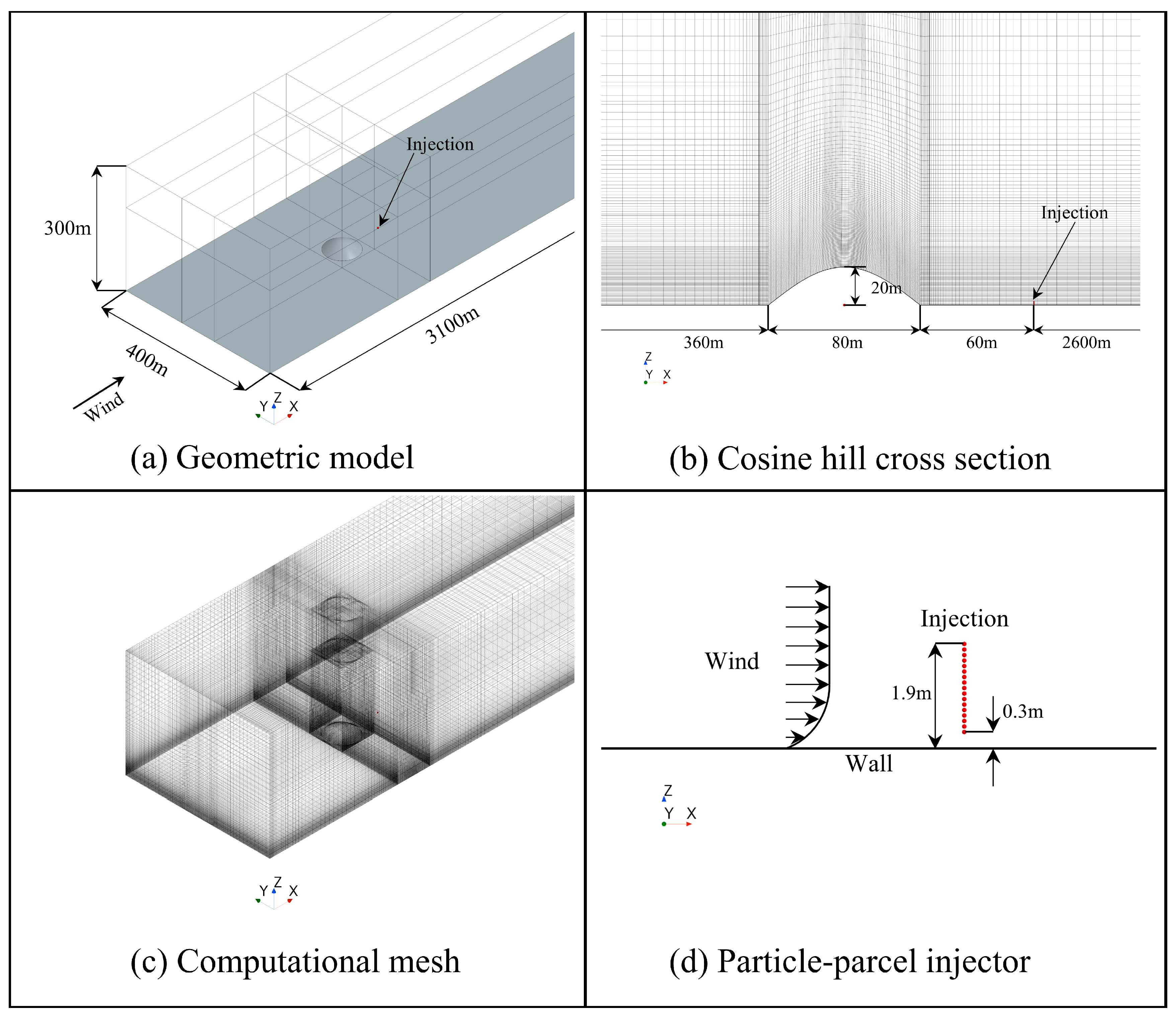
As shown in Figure 1a, the geometric model used to compute the flow fields under different atmospheric stability conditions has a length of 3100 m, a width of 400 m, and a height of 300 m. As shown in Figure 1b, the cosine-hill mesh cross-section has a basal diameter of 80 m and a height of 20 m, and the windward slope is located 360 m downstream of the left velocity inlet. As shown in Figure 1c, the computational mesh is locally refined within a region of 90 m × 90 m × 200 m around the cosine hill, and the full mesh is generated by applying oriented stretching with double-sided hyperbolic functions in five directions. As shown in Figure 1d, the particle-parcel injector consists of 17 release points; the highest and lowest points are located 1.9 m and 0.3 m above the ground, respectively, and adjacent release points are spaced at 0.1 m. The particle injector is positioned 60 m downstream of the leeward slope of the cosine hill and 2600 m upstream of the outlet.

Figure 1. Computational domain for simulating flow fields under different atmospheric stability conditions.

As shown in Figure 1a, the left boundary was specified as a velocity inlet, with inlet conditions prescribed according to Equations (2), (3), (7) and (8). The right boundary was set as a pressure outlet, the bottom boundary was treated as a wall, and the remaining boundaries were specified as symmetry planes. The air density ${\rho }_a$ was set to 1.225 kg/m³, the reference height $z_{refer}$ was set to 10 m, the momentum roughness length $z_0$ was set to 2.0 × 10⁻³ m, and the thermal roughness length $z_{0h}$ was set to 2.0 × 10⁻⁵ m. The friction velocity $u_{*}$ and surface potential temperature ${\theta }_s$ were obtained by substituting the wind speed and potential temperature at $z_{refer}$ into Equations (2) and (3), respectively. The potential temperature scale ${\theta }_{*}$ was then calculated using Equation (16) [38]. The conversion between potential temperature and temperature followed Equation (17) [39], where $p_0$ denotes the standard atmospheric pressure and $p$ denotes the atmospheric pressure at the specified elevation.

$${\theta }_{*}={\displaystyle \frac{-H}{\rho c_p{u}_{*}}}$$

(16)

$$\theta =T{\left({\displaystyle \frac{p_0}{p}}\right)}^{0.286}$$

(17)

2.4. Grid Independence Analysis

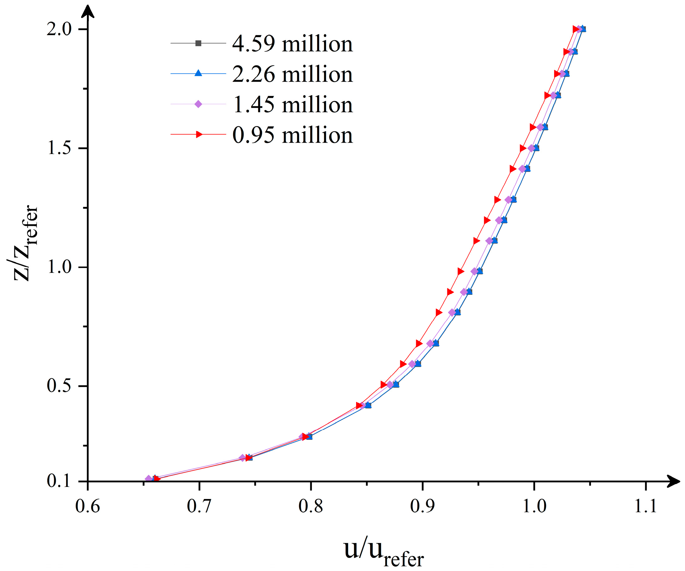
Based on the mesh-generation scheme described above, four meshes with different resolutions were generated, containing 950,000, 1.45 million, 2.26 million, and 4.59 million cells, respectively. These grids were used to perform numerical simulations under the same conditions (Table 2). The dimensionless velocity was taken at different heights 300 m from the inlet. As shown in Figure 2, when the grid numbers were 950,000 and 1.45 million, there was a noticeable discrepancy in the dimensionless velocities. As the grid resolution increased, when the grid numbers reached 2.26 million and 4.59 million, the two dimensionless velocity curves almost coincided. This indicates that further increasing the grid resolution beyond 2.26 million cells had little effect on the numerical simulation results. Therefore, a grid with 2.26 million cells was chosen for further study to meet the computational accuracy requirements.

Table 2. Basic parameter settings for the grid-independence test.

$\mathit{L}$ [m]	${\mathit{\rho }}_{\mathit{a}}$ [kg/m3]	${\mathit{z}}_{\mathit{r}\mathit{e}\mathit{f}\mathit{e}\mathit{r}}$ [m]	${\mathit{u}}_{\mathit{r}\mathit{e}\mathit{f}\mathit{e}\mathit{r}}$ [m/s]	${\mathit{\theta }}_{\mathit{r}\mathit{e}\mathit{f}\mathit{e}\mathit{r}}$ [K]	$\mathit{H}$ [W/m2]
$\pm \infty$	1.225	10	6.5	288	0

Figure 2. Grid-independence test.

2.5. Wind-Field Construction and Dust-Particle Transport Simulation

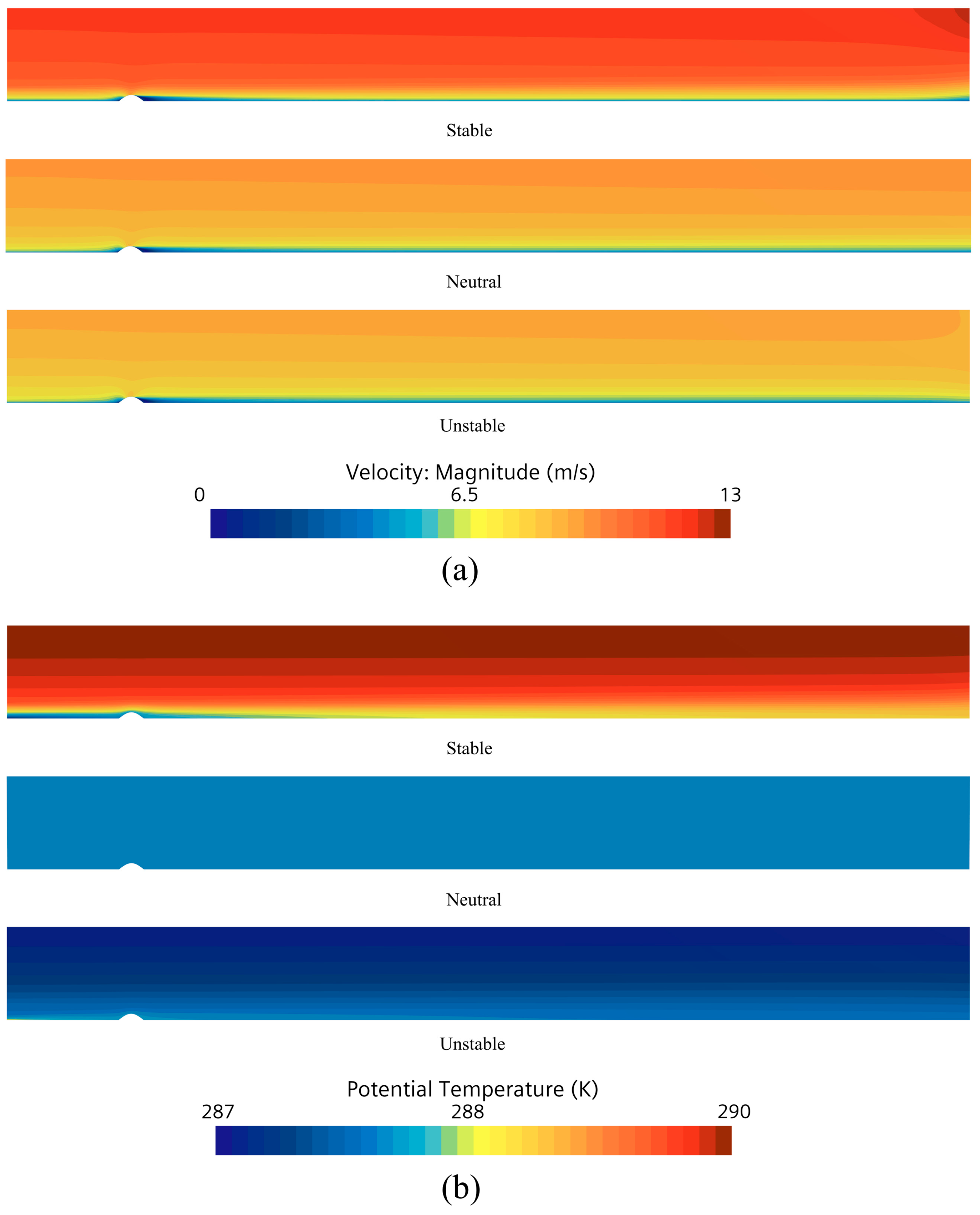
Based on the standard k-ε turbulence model, the Boussinesq model, and the atmospheric-stability formulation, the flow field over the meshed domain was computed to obtain flow fields under stable, neutral, and unstable conditions (Figure 3).

Figure 3. Contours of wind speed and potential temperature under different atmospheric stability conditions: (a) wind speed; (b) potential temperature.

Subsequently, Lagrangian particle parcels were injected into the flow field using the injector shown in Figure 1d. For the injection procedure, the release-point array emitted a total of $N_{inj}$ particle parcels along the wind direction at each time step, and these $N_{inj}$ particle parcels were allocated to the 17 release points according to the distribution described by Equations (18) and (19). This allocation follows the commonly used exponential vertical profile of horizontal saltation flux [40].

$$f_d=f_0\cdot e^{-\lambda (z-z_{sal})}$$

(18)

$$N_z=N_{inj}\times {\displaystyle \frac{{\displaystyle {\int }_z^{z+0.1}{f}_0\cdot e^{-\lambda (z-z_{sal})}}}{{\displaystyle {\int }_{z_{sal}}^2{f}_0\cdot e^{-\lambda (z-z_{sal})}}}}$$

(19)

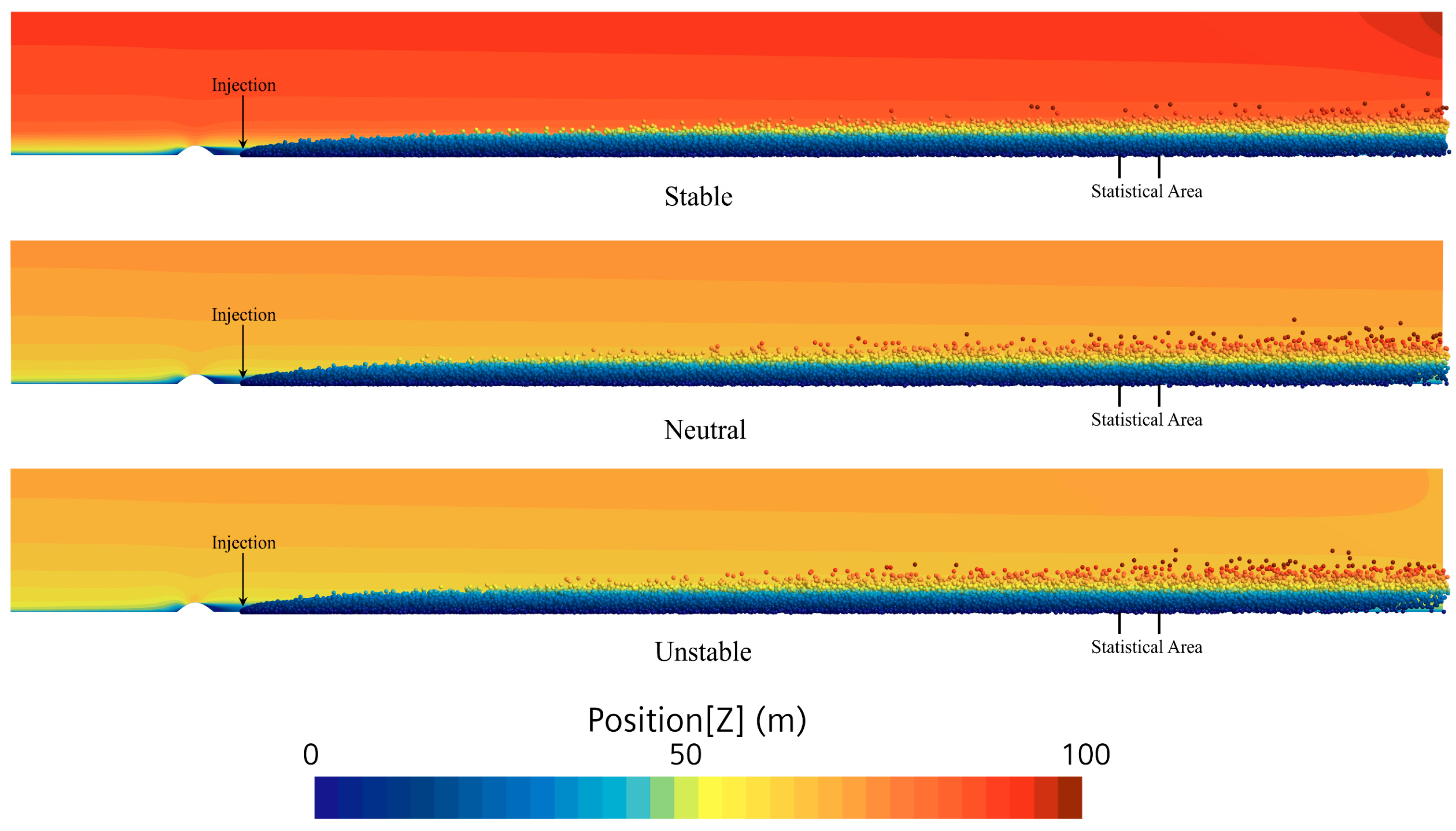
Here, $z$ is the height of each release point, $N_z$ is the number of particle parcels released from each point per time step, $f_d$ is the horizontal sand-flux density at the corresponding height, and $z_{sal}$ is the saltation-layer height (set to 0.3 m in this study). $f_0$ denotes the horizontal sand-flux density at $z$ = $z_{sal}$, where $f_0=m_0/(A\cdot T)$; $m_0$ is the mass of dust collected through area $A$ within time $T$. The value of $N_{inj}$ was set to 500, and λ was set to 1; therefore, 58 particle parcels were released at $z$ = 0.3 m per time step, while 12 particle parcels were released at $z$ = 1.9 m per time step. The computational time step was 0.2 s, and the simulation was run for 400 s; a total of 500 particle parcels were released at each time step until the end of the simulation. The Lagrangian-phase parameters were set as follows: ${\rho }_{dust}$ = 2650 kg/m³ and $d_{dust}$ = 10 $\mathrm{\mu }\mathrm{m}$. When a particle parcel contacted the bottom wall, it was automatically removed from the calculation. After all time steps were completed, the distribution of particle parcels on the x–z plane was sampled within the range 1900–2000 m downstream of the injector (where the dust cloud had entered a steady suspension stage), and the vertical distribution characteristics of the dust cloud were further analyzed. As shown in Figure 4, dust transport was simulated based on the wind-speed field shown in Figure 3a, and the color scale represents the height of the particles above the bottom wall.

Figure 4. Suspension transport of the dust cloud.

3. Results and Discussion

Three sets of cases were designed by varying the Monin–Obukhov length $L$, the reference wind speed $u_{refer}$, and the air density ${\rho }_a$ (representing plateau conditions). By compiling the coordinate information of the dust cloud within the sampling region shown in Figure 4 for each case, the relative-density maps of the dust cloud were obtained from the simulations. Together with the potential temperature scale ${\theta }_{*}$ and the number of particle parcels within the sampling region $N_{sta}$, the near-surface spatial distribution characteristics and patterns of the dust cloud were analyzed.

3.1. Results and Discussion Under Different Monin–Obukhov Lengths

In this subsection, 15 cases were considered. All cases shared the same values of ${\rho }_a$, $z_{refer}$, $u_{refer}$ and ${\theta }_{refer}$, while only the Monin–Obukhov length was varied (Table 3). The cases covered atmospheric stability regimes ranging from strongly stable to neutral and then to strongly unstable. After the simulations were completed, the near-surface spatial distribution characteristics of the dust cloud under different Monin–Obukhov lengths $L$ were analyzed.

Table 3. Simulation cases with different Monin–Obukhov lengths ($L$).

Case	$\mathit{L}$ [m]	${\mathit{\rho }}_{\mathit{a}}$ [kg/m3]	${\mathit{z}}_{\mathit{r}\mathit{e}\mathit{f}\mathit{e}\mathit{r}}$ [m]	${\mathit{u}}_{\mathit{r}\mathit{e}\mathit{f}\mathit{e}\mathit{r}}$ [m/s]	${\mathit{\theta }}_{\mathit{r}\mathit{e}\mathit{f}\mathit{e}\mathit{r}}$ [K]	$\mathit{H}$ [W/m2]
І-1	20	1.225	10	6.5	288	−62.386
І-2	30					−52.659
І-3	50					−38.711
І-4	80					−27.296
І-5	100					−22.757
І-6	200					−12.380
І-7	400					−6.463
І-8	$\pm \infty$					0
І-9	−400					6.969
І-10	−200					14.312
І-11	−100					29.893
І-12	−80					38.062
І-13	−50					63.829
І-14	−30					113.472
І-15	−20					181.053

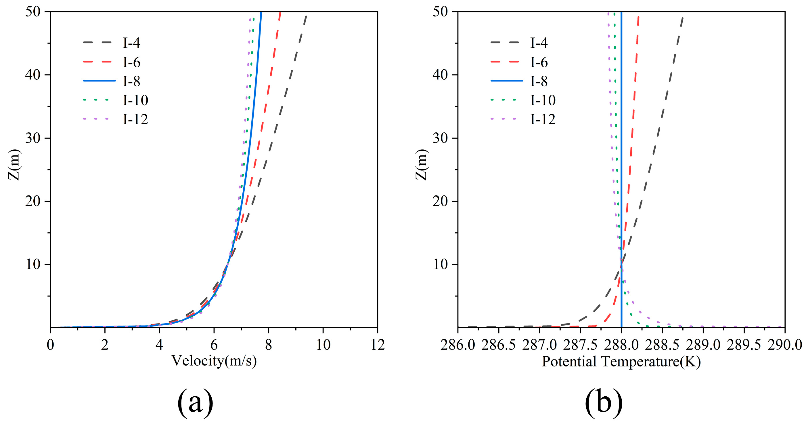
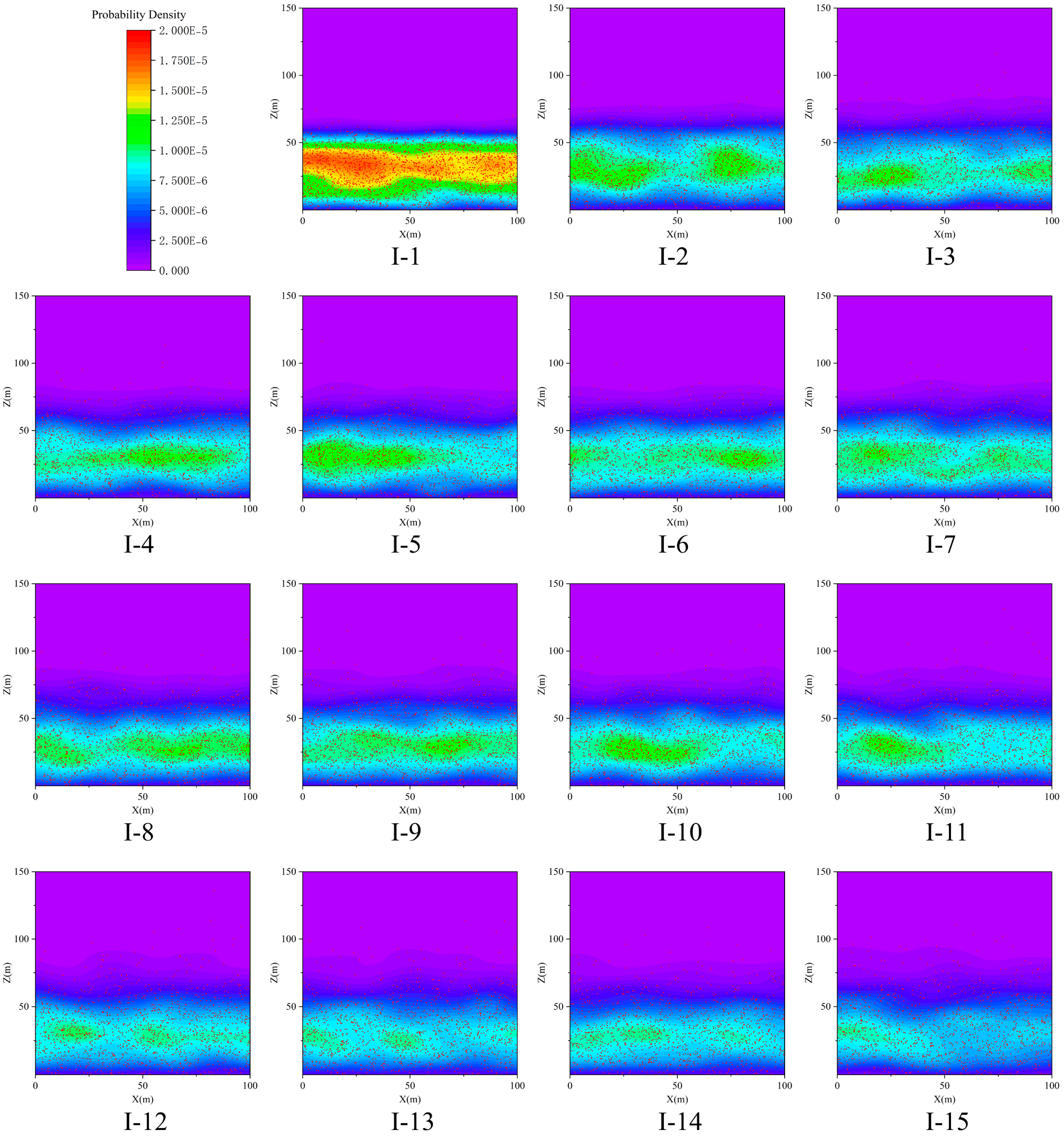
Figure 5 provides the inlet wind-speed and potential-temperature profiles for selected cases, which are used here to interpret the stability-dependent background states. Figure 6 presents the probability-density distributions of the dust cloud within the sampling region for all 15 cases, from which the near-surface accumulation pattern and the associated dispersion height are visually identified. As indicated in Figure 6, the near-surface distribution of the dust cloud differed markedly among cases with different $L$. Under stable conditions ($L$ > 0; Cases I-1 to I-7), compared with the neutral condition ($L$ = $\pm \infty$; Case I-8), the dust cloud exhibited higher concentrations and a lower dispersion height, and this tendency varied with increasing $L$: the larger $L$ became, the closer the concentration and dispersion height approached those of Case I-8. Under unstable conditions ($L$ < 0; Cases I-9 to I-15), compared with the neutral condition ($L$ = $\pm \infty$; Case I-8), the dust cloud exhibited lower concentrations and a higher dispersion height, and this tendency varied with decreasing $L$: the smaller $L$ became, the closer the concentration and dispersion height approached those of Case I-8.

Figure 5. Wind speed and potential temperature profiles for selected cases in Table 3: (a) wind speed; (b) potential temperature.

Figure 6. Probability density distributions of the dust cloud within the sampling region for the 15 cases with different Monin–Obukhov lengths ($L$).

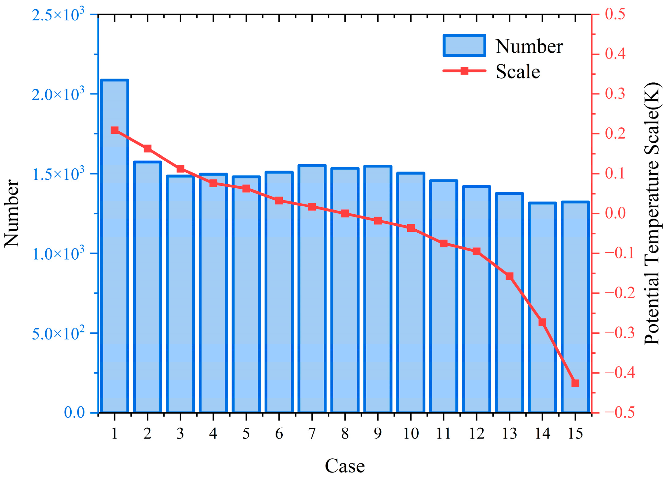
Figure 7 shows the variations in the potential temperature scale ${\theta }_{*}$ and the number of particle parcels within the sampling region, $N_{sta}$, across the 15 cases. Overall, ${\theta }_{*}$ and $N_{sta}$ decreased as L decreased from 20 m to −20 m. Specifically, within the interval [20, 50] (Cases I-1 to I-3), $N_{sta}$ decreased sharply; within the intervals [80, +∞] and [−∞, −200] (Cases I-4 to I-10), $N_{sta}$ showed only small fluctuations; and within the interval [−100, −20] (Cases I-11 to I-15), $N_{sta}$ decreased relatively sharply. Consistent with Figure 6, within [20, 50], the dust-cloud concentration decreased rapidly and the dispersion height increased rapidly; within [80, $+\infty$] and [$-\infty$, −200], the dust-cloud concentration and dispersion height were almost unchanged; within [−100, −20], the dust-cloud concentration decreased slowly and the dispersion height increased slowly. Similar simulation results were also reported by Wang [41]. To interpret the underlying mechanism, Figure 5 is further referenced to compare the stability-dependent inlet wind-speed and potential-temperature profiles, this behavior can be interpreted as follows: although ${\theta }_{*}$ varied more strongly under unstable conditions, compared with stable conditions the wind-speed and potential-temperature profiles differed only slightly from those under the neutral condition. Therefore, when $L$ < 0, as $L$ decreased, the dust-cloud concentration, dispersion height, and $N_{sta}$ differed only marginally from those under $L$ = $\pm \infty$, and the weakening trend was also slow.

Figure 7. Variations in the potential temperature scale (${\theta }_{*}$) and the number of particle parcels within the sampling region ($N_{sta}$) across the 15 cases.

3.2. Results and Discussion Under Different Reference Wind Speeds

In this subsection, 12 cases were considered, including four cases each under stable, neutral, and unstable conditions. All cases shared the same Monin–Obukhov length $L$, ${\rho }_a$, $z_{refer}$ and ${\theta }_{refer}$, whereas only the reference wind speed $u_{refer}$ was varied (Table 4). After the simulations were completed, the near-surface spatial distribution characteristics of the dust cloud under different $u_{refer}$ were analyzed.

Table 4. Simulation cases with different reference wind speeds ($u_{refer}$).

Case	$\mathit{L}$ [m]	${\mathit{\rho }}_{\mathit{a}}$ [kg/m3]	${\mathit{z}}_{\mathit{r}\mathit{e}\mathit{f}\mathit{e}\mathit{r}}$ [m]	${\mathit{u}}_{\mathit{r}\mathit{e}\mathit{f}\mathit{e}\mathit{r}}$ [m/s]	${\mathit{\theta }}_{\mathit{r}\mathit{e}\mathit{f}\mathit{e}\mathit{r}}$ [K]	$\mathit{H}$ [W/m2]
II-1	80	1.225	10	8.5	288	−61.039
II-2	80			7.5		−41.931
II-3	80			6.5		−27.296
II-4	80			5.5		−16.536
II-5	$\pm \infty$			8.5		0
II-6	$\pm \infty$			7.5		0
II-7	$\pm \infty$			6.5		0
II-8	$\pm \infty$			5.5		0
II-9	−80			8.5		85.115
II-10	−80			7.5		58.470
II-11	−80			6.5		38.062
II-12	−80			5.5		23.059

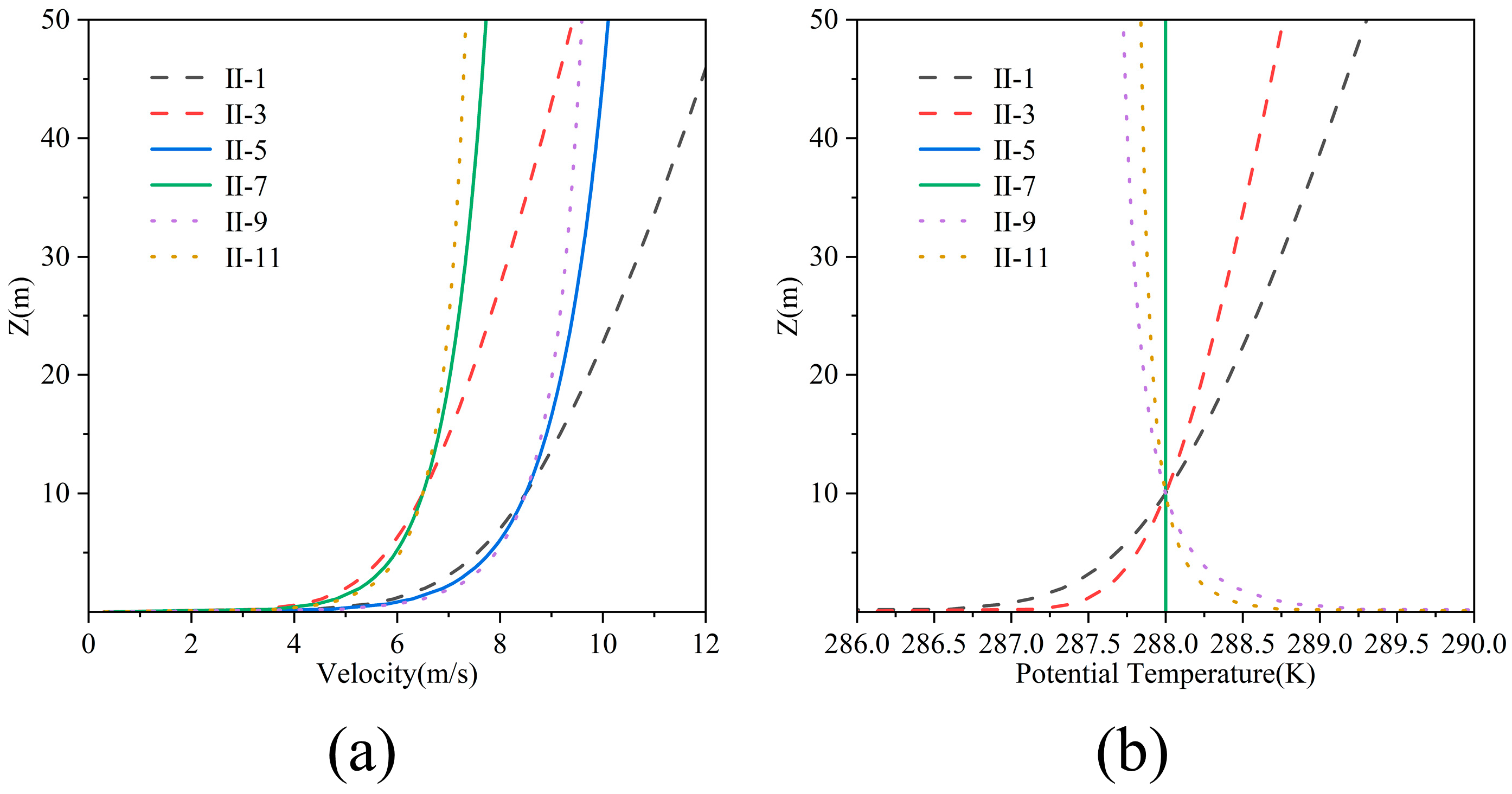
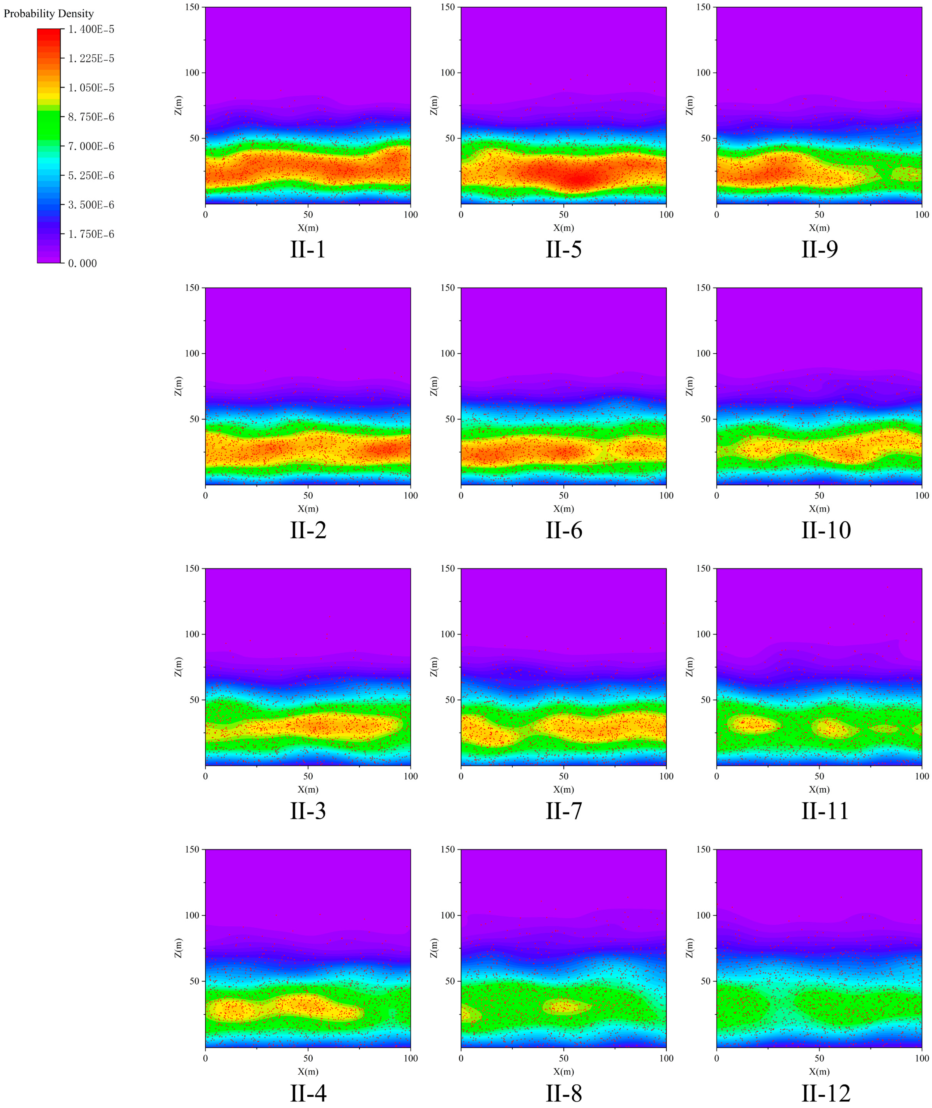
Figure 8 shows the inlet wind-speed and potential-temperature profiles for selected cases and is used to interpret the stability-dependent background states. Figure 9 provides visual evidence in the sampling region, where near-surface probability density and dispersion height are compared across the 12 cases. As indicated in Figure 9, the near-surface distribution of the dust cloud differed markedly among cases with different $u_{refer}$. Under stable (Cases II-1 to II-4), neutral (Cases II-5 to II-8), and unstable (Cases II-9 to II-12) conditions, the dust-cloud concentration increased as $u_{refer}$ increased. In addition, the concentration in Case II-5 was higher than those in Cases II-2 to II-4; the concentration in Case II-9 was higher than those in Cases II-7 to II-8; and the concentration in Case II-10 was higher than that in Case II-8. These results indicate that, in addition to atmospheric stability, the reference wind speed is also an important factor affecting the dust-cloud concentration.

Figure 8. Wind speed and potential temperature profiles for selected cases in Table 4: (a) wind speed; (b) potential temperature.

Figure 9. Probability density distributions of the dust cloud within the sampling region for the 12 cases with different reference wind speeds ($u_{refer}$).

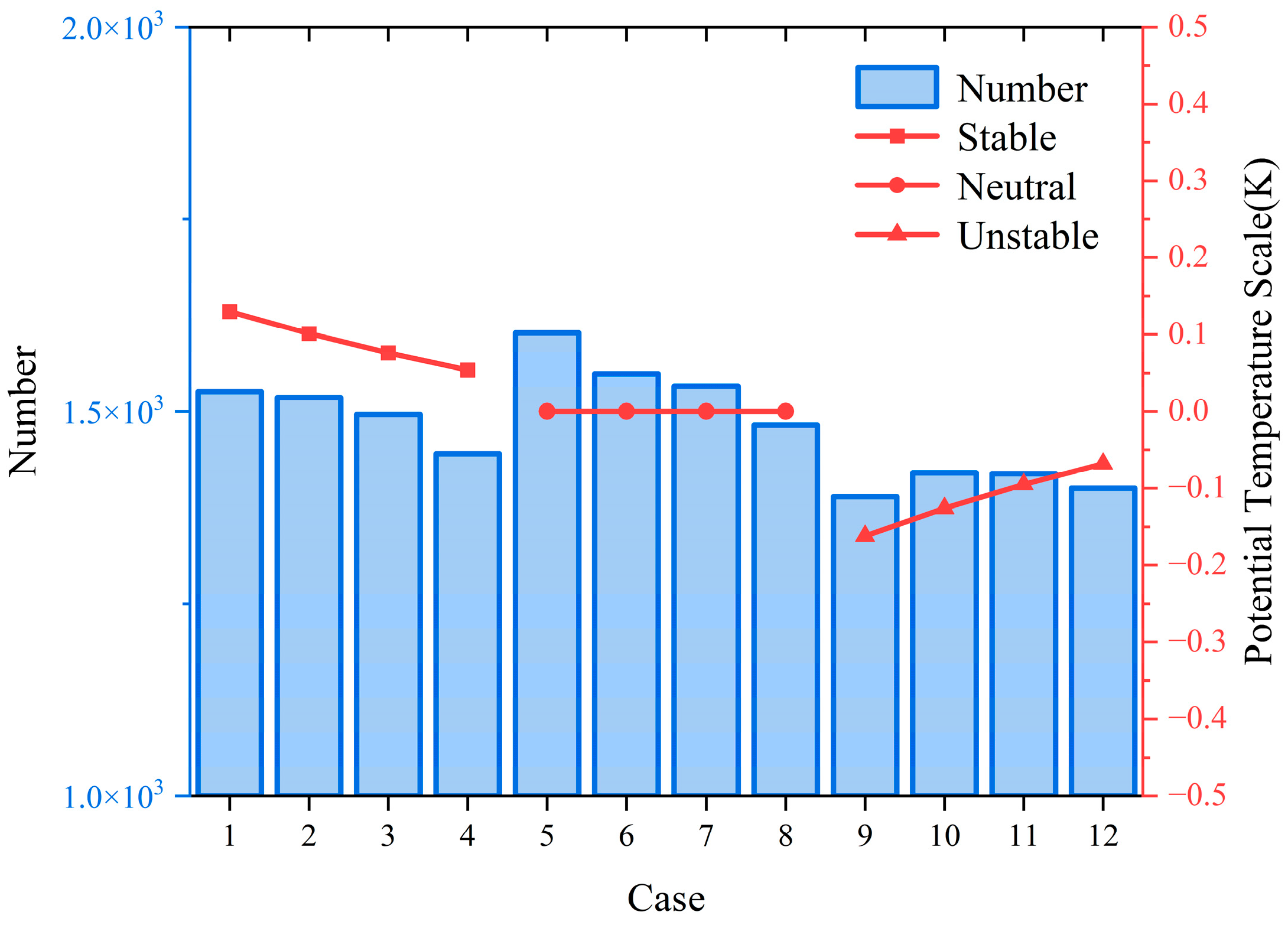
Figure 10 shows the variations in the potential temperature scale ${\theta }_{*}$ and the number of particle parcels within the sampling region, $N_{sta}$, across the 12 cases. Under stable conditions (Cases II-1 to II-4), ${\theta }_{*}$ and $N_{sta}$ increased slowly as $u_{refer}$ increased. Under neutral conditions (Cases II-5 to II-8), ${\theta }_{*}$ remained unchanged, whereas $N_{sta}$ increased rapidly as $u_{refer}$ increased. Under unstable conditions (Cases II-9 to II-12), ${\theta }_{*}$ decreased as $u_{refer}$ increased, while $N_{sta}$ remained nearly constant. This behavior can be interpreted as follows: under neutral conditions, in the absence of thermal buoyancy, increasing $u_{refer}$ enhanced turbulence, making the dust cloud less prone to settling; under stable conditions, thermal buoyancy suppressed the strengthening of turbulence; therefore, $N_{sta}$ increased more slowly with $u_{refer}$; under unstable conditions, the potential-temperature profiles among cases were similar (Figure 8b); thus, $N_{sta}$ changed little. A further observation from Figure 9 was that, under unstable conditions, as $u_{refer}$ increased, ${\theta }_{*}$ decreased (implying stronger buoyancy-driven turbulence), yet the dust-cloud concentration increased and the dispersion height decreased. This can be attributed to the limited effectiveness of thermal buoyancy in promoting dust dispersion under unstable conditions. Increasing $u_{refer}$ enhanced low-level turbulence, causing a large number of dust particles to undergo frequent cycles of uplift and deposition. As a result, many dust particles remained trapped at low altitudes, which in turn suppressed vertical dispersion, leading to a higher dust-cloud concentration and a lower dispersion height.

Figure 10. Variations in the potential temperature scale (${\theta }_{*}$) and the number of particle parcels within the sampling region ($N_{sta}$) across the 12 cases.

3.3. Results and Discussion Under Plain and Plateau Conditions

In this subsection, six cases were considered, including two cases each under stable, neutral, and unstable conditions. All cases shared the same Monin–Obukhov length $L$, $z_{refer}$ and $u_{refer}$, while only ${\rho }_a$ (plain versus plateau conditions) and ${\theta }_{refer}$ were varied (Table 5). After the simulations were completed, the computed results were used to analyze the near-surface spatial distribution characteristics of the dust cloud under plain and plateau conditions. For Cases III-2, III-4, and III-6, ${\theta }_{refer}$ was calculated using Equation (17), with $p$ set to 650 hPa to represent the atmospheric pressure in Lhasa. The two values of ${\theta }_{refer}$ in Table 5 essentially corresponded to the same ambient temperature (15 °C).

Table 5. Simulation cases under plain and plateau conditions.

Case	$\mathit{L}$ [m]	${\mathit{\rho }}_{\mathit{a}}$ [kg/m3]	${\mathit{z}}_{\mathit{r}\mathit{e}\mathit{f}\mathit{e}\mathit{r}}$ [m]	${\mathit{u}}_{\mathit{r}\mathit{e}\mathit{f}\mathit{e}\mathit{r}}$ [m/s]	${\mathit{\theta }}_{\mathit{r}\mathit{e}\mathit{f}\mathit{e}\mathit{r}}$ [K]	$\mathit{H}$ [W/m2]
III-1	80	1.225	10	6.5	288	−27.296
III-2		0.81			323.411	−20.268
III-3	$\pm \infty$	1.225			288	0
III-4		0.81			323.411	0
III-5	−80	1.225			288	38.062
III-6		0.81			323.411	28.262

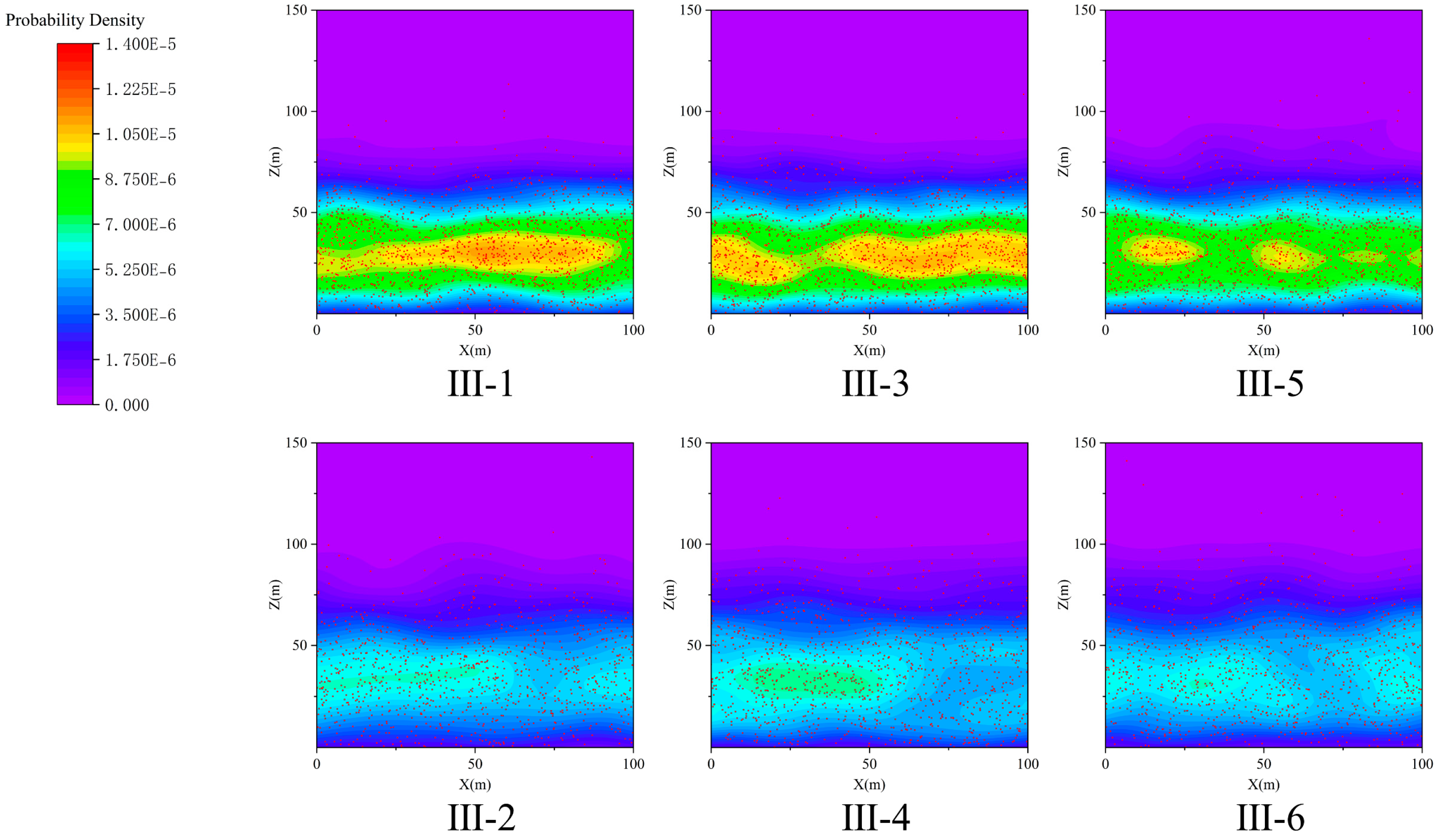
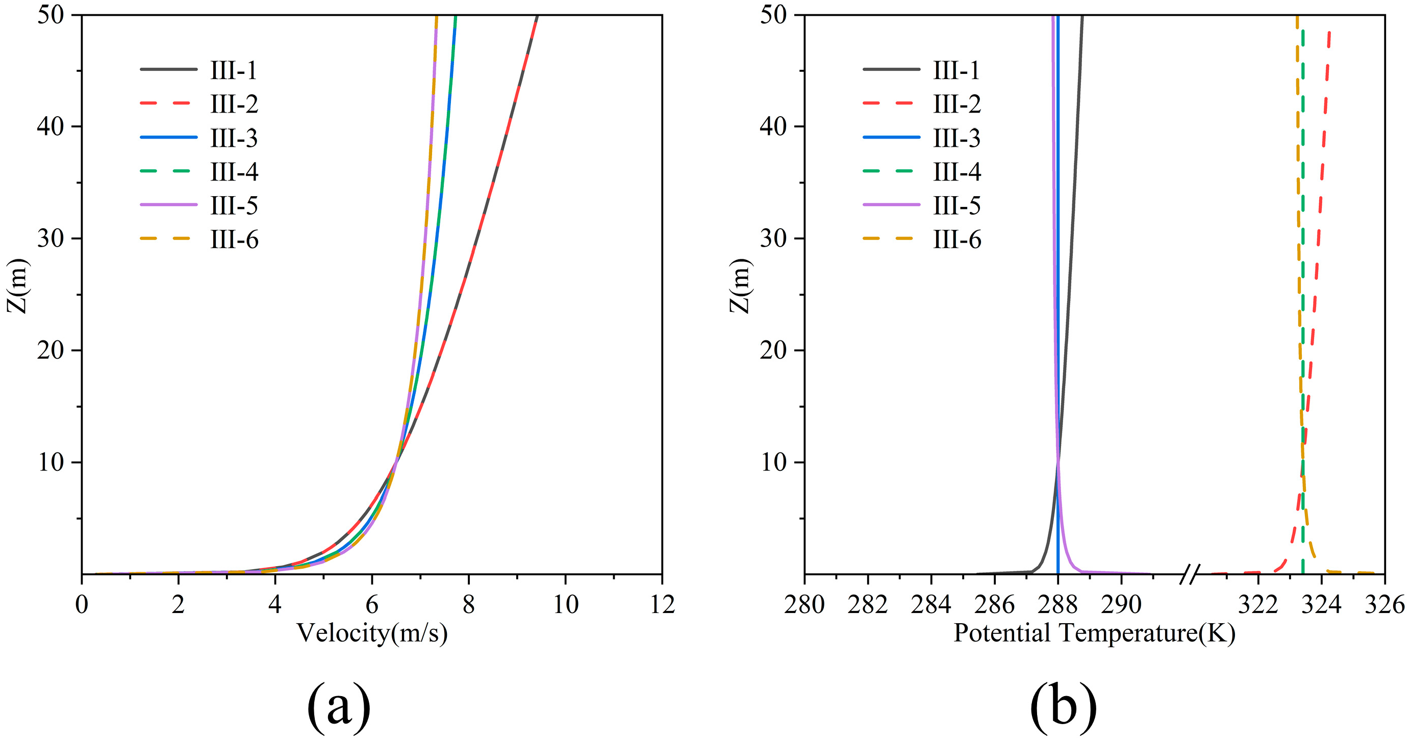
Figure 11 shows the wind-speed and potential-temperature profiles for the above cases. The plain cases (Cases III-1, III-3, and III-5) and the plateau cases (Cases III-2, III-4, and III-6) had identical wind-speed profiles, whereas their potential-temperature profiles differed substantially. Figure 12 shows the probability-density distributions of the dust cloud within the sampling region for the six cases in Table 5. As shown in Figure 12, under different atmospheric stability conditions, the plateau cases exhibited lower dust-cloud concentrations and a higher dispersion height than the corresponding plain cases.

Figure 11. Wind speed and potential temperature profiles for the cases in Table 5: (a) wind speed; (b) potential temperature.

Figure 12. Probability density distributions of the dust cloud within the sampling region for the plain and plateau cases.

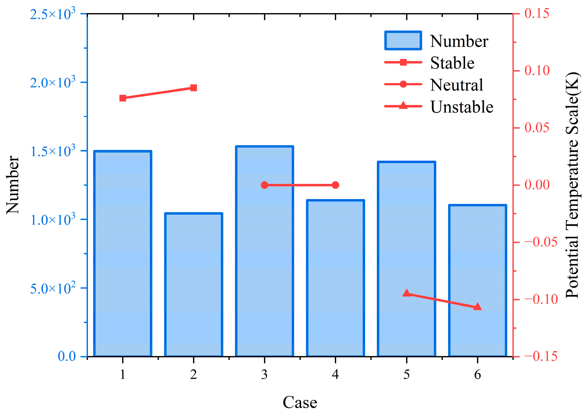
Figure 13 shows the variations in the potential temperature scale ${\theta }_{*}$ and the number of particle parcels within the sampling region, $N_{sta}$, across the six cases. Under neutral conditions (Cases III-3 to III-4), ${\theta }_{*}$ remained unchanged, whereas $N_{sta}$ decreased under plateau conditions relative to plain conditions. Under stable (Cases III-1 to III-2) and unstable conditions (Cases III-5 to III-6), ${\theta }_{*}$ varied only slightly, but $N_{sta}$ still decreased markedly. Together with Figure 11b, these results indicate that although the entire potential-temperature profile increased substantially under plateau conditions relative to plain conditions, the resulting change in ${\theta }_{*}$ was limited; therefore, the potential-temperature difference was not the primary driver of the difference in $N_{sta}$. This behavior was attributed to weakened turbulence under plateau conditions due to reduced air density. Although some dust particles were lifted to higher altitudes by aerodynamic drag, the limited vertical transport capacity forced more particles to settle to the ground, thereby substantially reducing $N_{sta}$ under plateau conditions.

Figure 13. Variations in the potential temperature scale (${\theta }_{*}$) and the number of particle parcels within the sampling region ($N_{sta}$) across the six cases.

4. Conclusions

In this study, a near-field flow field containing an idealized cosine hill was constructed using computational fluid dynamics (CFD). Stable, neutral, and unstable stratification cases were prescribed at the inlet based on Monin–Obukhov similarity theory (MOST), and a Lagrangian particle approach was coupled to simulate the release and transport of dust particles. This study focuses on near-surface concentration patterns and dispersion-height variations to support the assessment of near-field blowing-sand impacts on short-range receptors. On this basis, the effects of the Obukhov length $L$, the reference wind speed $u_{refer}$, and the air density ${\rho }_a$ were examined, leading to the following conclusions:

(1)

Atmospheric stability is the primary factor controlling near-surface accumulation and vertical dispersion. As stability strengthens (i.e., as $\left|L\right|$ approaches $z_{refer}$), near-surface dust accumulation increases markedly and the dispersion height decreases rapidly. As instability strengthens, near-surface accumulation weakens and the dispersion height increases, although the sensitivity is weaker than that under stable stratification. When $\left|L\right|$ is relatively large (approximately ≥200 m), the dust-cloud characteristics gradually approach those under neutral conditions, indicating that the stability effect diminishes under weak stratification. Using the number of particle parcels in the sampling region $N_{sta}$ as a quantitative metric, relative to the neutral case (Case I-8), the variation range under stable stratification (Cases I-1 to I-7) is −3% to 38%, whereas that under unstable stratification (Cases I-9 to I-15) is −13% to 1%. These trends are consistent with the probability-density distributions in Figure 6.

(2)

The influence of the reference wind speed on dust-cloud structure exhibits pronounced stability dependence. As $u_{refer}$ increases, the dust cloud generally shows enhanced near-surface accumulation and a reduced dispersion height; however, the magnitude and underlying mechanisms differ across stability regimes. Based on the variation in $N_{sta}$, the relative changes in Cases II-2, II-3, and II-4 with respect to Case II-1 are relatively large under stable conditions; under neutral conditions, the relative changes in Cases II-6, II-7, and II-8 with respect to Case II-5 are even larger; whereas under unstable conditions, the relative changes in Cases II-10, II-11, and II-12 with respect to Case II-9 are small and nearly unchanged. In particular, stronger winds tend to suppress vertical spreading under unstable conditions, while under stable conditions, they intensify buoyancy-related suppression of dispersion, leading to more pronounced near-surface accumulation.

(3)

Air density has a non-negligible impact on near-field blowing-sand assessment and should be explicitly considered in plateau environments. Compared with plain conditions, lower air density under plateau conditions weakens the near-surface probability density of the dust cloud and increases the dispersion height. According to the quantitative results in Figure 13, relative to plain conditions, $N_{sta}$ under plateau conditions decreases markedly across all three stability regimes: by approximately 30% under stable conditions, 25% under neutral conditions, and 22% under unstable conditions. This “consistent and substantial reduction across stability regimes” supports the mechanistic interpretation that reduced air density weakens turbulence intensity and limits vertical transport capacity, thereby promoting particle settling and reducing the number of particle parcels within the sampling region.

The CFD-Lagrangian particle simulation framework proposed in this study, together with the “near-surface concentration–dispersion height” indicator system, can provide a methodological reference for the rapid interpretation and risk comparison of near-field blowing-sand impacts over complex terrain, and is particularly applicable to local windblown-sand impact assessment and sensitivity analysis for short-range receptors. It should be noted that the idealized cosine hill was adopted to highlight the underlying mechanisms; real-world complexities such as multi-scale terrain undulations, heterogeneous surface roughness, and spatially variable dust sources were not considered. Future work will incorporate realistic topography and measurement validation to quantify uncertainty and improve transferability.

References

- Shao, Y.; Dong, C. A review on East Asian dust storm climate, modelling and monitoring. Glob. Planet. Change 2006, 52, 1–22. [Google Scholar] [CrossRef] [Scilit]
- Wang, W.; Fang, Z. Sand and dust storm weather and research progress: A review. J. Appl. Meteorol. Sci. 2004, 15, 366–381. [Google Scholar]
- Yin, Z.; Zhao, Z.; Zhang, X.; Meng, L. Aerosol characteristics during blowing-sand and floating-dust events and their impacts on air quality. J. Agric. Catastrophology 2025, 15, 320–322. [Google Scholar]
- Aishajiang, A.; Xu, H.; Kasim, T.; Abulikemu, A. Origin and transport pathway of dust storm and its contribution to particulate air pollution in northeast edge of Taklimakan Desert, China. Atmosphere 2021, 12, 113. [Google Scholar] [CrossRef] [Scilit]
- Grell, G.A.; Peckham, S.E.; Schmitz, R.; McKeen, S.A.; Frost, G.; Skamarock, W.C.; Eder, B. Fully coupled “online” chemistry within the WRF model. Atmos. Environ. 2005, 39, 6957–6975. [Google Scholar] [CrossRef] [Scilit]
- Mamun, A.A.; Chen, Y.; Liang, J. Radiative and cloud microphysical effects of the Saharan dust simulated by the WRF-Chem model. J. Atmos. Sol.-Terr. Phys. 2021, 219, 105646. [Google Scholar] [CrossRef] [Scilit]
- Spyrou, C.; Solomos, S.; Bartsotas, N.S.; Douvis, K.C.; Nickovic, S. Development of a dust source map for WRF-Chem model based on MODIS NDVI. Atmosphere 2022, 13, 868. [Google Scholar] [CrossRef] [Scilit]
- Hamidi, M.; Kavianpour, M.R.; Shao, Y. Numerical simulation of dust events in the Middle East. Aeolian Res. 2014, 13, 59–70. [Google Scholar] [CrossRef] [Scilit]
- LeGrand, S.L.; Polashenski, C.; Letcher, T.W.; Creighton, G.A.; Peckham, S.E.; Cetola, J.D. The AFWA dust emission scheme for the GOCART aerosol model in WRF-Chem v3.8.1. Geosci. Model Dev. 2019, 12, 131–166. [Google Scholar] [CrossRef] [Scilit]
- Meroney, R.; Ohba, R.; Leitl, B.; Kondo, H.; Grawe, D.; Tominaga, Y. Review of CFD guidelines for dispersion modeling. Fluids 2016, 1, 14. [Google Scholar] [CrossRef] [Scilit]
- Ma, X.; Zhong, W. CFD-DPM simulation on the atmospheric pollutant dispersion in industrial park. Atmosphere 2024, 15, 298. [Google Scholar] [CrossRef] [Scilit]
- Kim, D.; Chin, M.; Kemp, E.M.; Tao, Z.; Peters-Lidard, C.D.; Ginoux, P. Development of high-resolution dynamic dust source function—A case study with a strong dust storm in a regional model. Atmos. Environ. 2017, 159, 11–25. [Google Scholar] [CrossRef] [Scilit] [PubMed]
- Anisimov, A.; Axisa, D.; Kucera, P.A.; Mostamandi, S.; Stenchikov, G. Observations and cloud-resolving modeling of haboob dust storms over the Arabian Peninsula. J. Geophys. Res. Atmos. 2018, 123, 12147–12179. [Google Scholar] [CrossRef] [Scilit]
- Hamzeh, H.N.; Abadi, S.R.A.; Kaskaoutis, G.D.; Mirzaei, E.; Shukurov, K.A.; Sotiropoulou, R.-E.P.; Tagaris, E. The importance of wind simulations over dried lake beds for dust emissions in the Middle East. Atmosphere 2024, 15, 24. [Google Scholar] [CrossRef] [Scilit]
- Jonassen, O.M.; Ólafsson, H.; Reuder, J.; Olseth, J.A. Multi-scale variability of winds in the complex topography of southwestern Norway. Tellus A Dyn. Meteorol. Oceanogr. 2012, 64, 11962. [Google Scholar] [CrossRef] [Scilit]
- Butler, W.B.; Wagenbrenner, S.N.; Forthofer, J.M.; Lamb, B.K.; Shannon, K.S.; Finn, D.; Eckman, R.M.; Clawson, K.; Bradshaw, L.; Sopko, P.; et al. High-resolution observations of the near-surface wind field over an isolated mountain and in a steep river canyon. Atmos. Chem. Phys. 2015, 15, 3785–3801. [Google Scholar] [CrossRef] [Scilit]
- Zhang, F.; Shi, X.; Zeng, C.; Wang, G.; Chen, Y. Changes in river sediment load over the Qinghai–Tibet Plateau and its influencing factors. Bull. Chin. Acad. Sci. 2019, 34, 1274–1284. [Google Scholar] [CrossRef]
- Liu, Y.; Wang, Y.; Shen, T. Spatial distribution and formation mechanism of aeolian sand in the middle reaches of the Yarlung Zangbo River. J. Mt. Sci. 2019, 16, 1987–2000. [Google Scholar] [CrossRef] [Scilit]
- Li, T.; Zhang, J.; Wu, Y.; Du, S.; Mo, D.; Liao, Y.; Chen, Z.; Liu, J.; Li, Q. Holocene aeolian activities linked to Indian summer monsoon in the middle reaches of the Yarlung Zangbo River. J. Geogr. Sci. 2020, 30, 2002–2014. [Google Scholar] [CrossRef] [Scilit]
- Tominaga, Y.; Stathopoulos, T. CFD simulation of near-field pollutant dispersion in the urban environment: A review of current modeling techniques. Atmos. Environ. 2013, 79, 716–730. [Google Scholar] [CrossRef] [Scilit]
- Joseph, G.; Lowndes, I.; Hargreaves, D. A computational study of particulate emissions from Old Moor Quarry, UK. J. Wind Eng. Ind. Aerodyn. 2018, 172, 68–84. [Google Scholar] [CrossRef] [Scilit]
- Silvester, S.; Lowndes, I.; Hargreaves, D. A computational study of particulate emissions from an open pit quarry under neutral atmospheric conditions. Atmos. Environ. 2009, 43, 6415–6424. [Google Scholar] [CrossRef] [Scilit]
- Liu, C.; Liu, H.; Kunkel, G.G.; Li, D.; Finn, D. Turbulence structures in the very stable boundary layer under the influence of wind profile distortion. J. Geophys. Res. Atmos. 2022, 127, e2022JD036565. [Google Scholar] [CrossRef] [Scilit]
- Debolskiy, A.V.; Mortikov, E.V.; Glazunov, A.V.; Lüpkes, C. Evaluation of surface layer stability functions and their extension to first-order turbulent closures for weakly and strongly stratified stable boundary layer. Bound.-Layer Meteorol. 2023, 187, 73–93. [Google Scholar] [CrossRef] [Scilit]
- Prabhakar, N.; Singh, P.; Sharma, M.; Mishra, S.K. An update to WRF surface layer parameterization over an Indian region. Dyn. Atmos. Ocean. 2024, 105, 101414. [Google Scholar] [CrossRef] [Scilit]
- Tran, V.; Ng, K.Y.E.; Skote, M. CFD simulation of dense gas dispersion in neutral atmospheric boundary layer with OpenFOAM. Meteorol. Atmos. Phys. 2020, 132, 273–285. [Google Scholar] [CrossRef] [Scilit]
- Pieterse, J.; Harms, T. CFD investigation of the atmospheric boundary layer under different thermal stability conditions. J. Wind Eng. Ind. Aerodyn. 2013, 121, 82–97. [Google Scholar] [CrossRef] [Scilit]
- Lu, H.; Shao, Y. A new model for dust emission by saltation bombardment. J. Geophys. Res. Atmos. 1999, 104, 16827–16842. [Google Scholar] [CrossRef] [Scilit]
- Taylor, P.A. Yaping Shao. Physics and modelling of wind erosion. Bound.-Layer Meteorol. 2001, 101, 127–128. [Google Scholar] [CrossRef] [Scilit]
- Tan, L.; Qu, J.; Wang, T.; Zhang, W.; Zhao, S.; Wang, H. Vertical flux density and frequency profiles of wind-blown sand as a function of the grain size over gobi and implications for aeolian transport processes. Aeolian Res. 2022, 55, 100787. [Google Scholar] [CrossRef] [Scilit]
- Tan, L.; Wang, H.; An, Z.; Qu, J. Aeolian sand transport over a dry playa surface: Sand flux density profiles, saltation layer height, and flux scaling laws and implications for dust emission dynamics. Catena 2023, 224, 106970. [Google Scholar] [CrossRef] [Scilit]
- Rogula, J.; Dzierżek, M. Vertical profiles of aeolian mass flux above different sand surfaces and sand surfaces covered with pebbles. Catena 2022, 212, 106006. [Google Scholar] [CrossRef] [Scilit]
- Wang, H.S.; Blocken, B.; Lin, Z. CFD simulation of the stratified atmospheric boundary layer: Consistency between Monin-Obukhov similarity theory and the standard k-ε model. Build. Environ. 2025, 267, 112284. [Google Scholar] [CrossRef] [Scilit]
- Dyer, A.J. A review of flux-profile relationships. Bound.-Layer Meteorol. 1974, 7, 363–372. [Google Scholar] [CrossRef] [Scilit]
- Alinot, C.; Masson, C. k–ε model for the atmospheric boundary layer under various thermal stratifications. J. Sol. Energy Eng. 2005, 127, 438–443. [Google Scholar] [CrossRef] [Scilit]
- Lai, J.K.; Merzari, E.; Hassan, Y.A. Sensitivity analyses in a buoyancy-driven closed system with high resolution CFD using Boussinesq approximation and variable density models. Int. J. Heat Fluid Flow 2019, 75, 1–13. [Google Scholar] [CrossRef] [Scilit]
- Talebmoustaph, C.; Fede, P.; Simonin, O.; Pallud, M.; Maheshwari, P. Stochastic Lagrangian wall deposition model for RANS prediction of deposition in turbulent gas–solid flows. Int. J. Multiph. Flow 2024, 178, 14. [Google Scholar] [CrossRef] [Scilit]
- Yano, J.; Wacławczyk, M. Nondimensionalization of the Atmospheric Boundary-Layer System: Obukhov Length and Monin-Obukhov Similarity Theory. Bound.-Layer Meteorol. 2021, 182, 417–439. [Google Scholar] [CrossRef] [Scilit]
- Baumgartner, M.; Weigel, R.; Harvey, A.H.; Plöger, F.; Achatz, U.; Spichtinger, P. Reappraising the appropriate calculation of a common meteorological quantity: Potential Temperature. Atmos. Chem. Phys. Discuss. 2020, 20, 15585–15616. [Google Scholar] [CrossRef] [Scilit]
- Sherman, D.J.; Bae, J.; Ellis, J.T.; Swann, C.; Parteli, E.J.R.; Farrell, E.; Li, B.; Araújo, A.D.; de Carvalho, A.M.; Sherman, D.L.; et al. Aeolian Saltation Flux Profiles: Comparison of Representation and Measurement Methods. Geosciences 2025, 15, 323. [Google Scholar] [CrossRef] [Scilit]
- Wang, X.; Yang, F.; Cui, P.; Huang, Y. Dispersion characteristics of pollutants within an urban building array under different atmospheric stability conditions. J. Subtrop. Resour. Environ. 2023, 18, 70–77. [Google Scholar] [CrossRef]
Disclaimer/Publisher’s Note: The statements, opinions and data contained in all publications are solely those of the individual author(s) and contributor(s) and not of MDPI and/or the editor(s). MDPI and/or the editor(s) disclaim responsibility for any injury to people or property resulting from any ideas, methods, instructions or products referred to in the content. |
© 2026 by the authors. Licensee MDPI, Basel, Switzerland. This article is an open access article distributed under the terms and conditions of the Creative Commons Attribution (CC BY) license.