Abstract
Community Earth System Model-Large Ensemble (CESM-LE) simulations are used to partition the Surface Air Temperature (SAT) trends over East Asia into the contribution of external forcing factors and internal variability. In the historical period (1966–2005), the summer SAT trends display a considerable diversity (≤−2 °C to ≥2 °C) across the 35 member ensembles, while under the RCP8.5 scenario, the region is mostly dominated by a strong warming trend (~1.5–2.5 °C/51 years) and touches the ~4 °C mark by the end of the 21st century. In the historical period, the warming is prominent over the Yangtze River basin of China, while under the RCP8.5 scenario, the warming pattern shifts northward towards Mongolia. In the historical period, the Signal-to-Noise Ratio (SNR) is less than 1, while it is higher than 4 under the RCP8.5 scenario, which indicates that, in the early period, internal variability overrides the forced response and vice versa under the RCP8.5 scenario. In addition, over much of the East Asian region, the chances of cooling are relatively high in the historical period, which partially counteracted the warming trend due to external forcing factors. In contrast, under the RCP8.5 scenario, the chances of warming reach ~100% over East Asia due to contributions from the external forcing factors. The novel aspect of the current study is that, in the negative phase (from the mid-1960s to ~2000), the Atlantic Multidecadal Oscillation (AMO) accounts for ~70–80% of the cooling trend or the SAT variability over East Asia, and thereafter, natural variability exhibits a slow increasing trend in the future. However, the contribution of external forcing factors increases from ~55% in 2000 to 95% in 2075 at a rate much faster than natural variability, which is primarily due to increasing downward solar radiation fluxes and albedo feedback on SAT over East Asia.
1. Introduction
The Earth’s climate change and its future trajectory [] are determined by the complex interaction between external forcing factors and internal variability. The unforced component within the climate system corresponds to internal variability that contributes significantly to the projected trends at the regional and global scales []. At multidecadal timescales, the contribution of external factors dominates over internal variability globally [,], while at regional scales, both factors contribute almost equally to the total climate trends [,,]. The observed trends can be considered as the coupled response of internal variability and externally forced responses driven by atmospheric circulation processes [,]. At the regional scale, internal variability often masks the footprint of anthropogenic climate change [,,,], and its predictability can only be improved by understanding the associated uncertainties related to its projections []. These uncertainties are arising mainly due to the forcing, model response and variabilities that are intrinsic to the climate system [,].
Here, we focused on SAT variability over East Asia (15–45° N and 100–140° E), which is under the active influence of the East Asian Summer Monsoon (EASM). Approximately one-third of the global population resides in East Asia, which includes mainland China, Japan, Korea, the Philippines and the Indochina peninsula. The southern and northern parts of China receive approximately 40~50% and 60~70% of the annual mean rainfall due to the EASM, respectively []. In the last quarter of the previous century, East Asian climate has experienced a weak EASM circulation [,], while in the late 1990s, another interdecadal shift towards a stronger EASM circulation has been identified []. This strengthening in monsoonal circulation is the consequence of a warming trend in the East Asian landmass []. Therefore, it is imperative to investigate the role of internal variability (AMO, ENSO, etc.), external forcing factors (GHG, aerosols, volcanic eruptions and solar variability) and the complex interactions between them that drive the SAT trend at different timescales.
Nath et al., (2019) [] has reported a close connection between the Atlantic Multidecadal Oscillation (AMO) and SAT variability at multidecadal timescales over Central India and over most of the Asian landmasses. Previous studies have shown that the long-term variabilities in the East Asian (e.g., China) climate are linked with global warming due to the increase in GHG emission [] from anthropogenic sources []. However, the magnitude of warming is not homogenous throughout the contiguous mainland of China and in East Asia as well. The warming trend varies widely from rapid warming in the east-central part of the region to a cooling trend in the northern and southern parts of East Asia. However, there is no consensus on the physical mechanisms (external forcings and/or internal variability) that are driving the long-term variabilities in monsoon and climate over East Asia [].
Decreasing albedo, increasing sensible heat fluxes and their impact on surface air temperature strongly influence the East Asian surface warming through several interconnected processes. A reduction in albedo due to increasing absorption of solar radiation is common in the urbanized areas or regions that are experiencing land use changes []. With more absorbed solar energy, the temperature of the surface rises, which increases the sensible heat flux by transferring more heat from the surface to the atmosphere. The combination of decreased albedo and increased sensible heat flux leads to a rise in surface air temperatures []. In East Asia, where urbanization [] and land use changes are prevalent, these effects can exacerbate local warming, influence climate patterns and potentially lead to more extreme weather events.
It is highly challenging to separate out the contribution of external forcing factors and internal variability from the total trend. Internal variability is arising due to uncertainties among the members due to a wide range of model sensitivities [,]. Standard deviations among the members and the ensemble mean are the measure of internal variability and external forcings, respectively. The contributions of external factors can be isolated from internal variability by employing a climate model with a large number (ensembles) of runs. Each member ensemble is subjected to the same external forcing, with a slight difference in its initial boundary condition, and is considered as the combination of intrinsic variability and externally forced responses. The contribution due to internal variability can be obtained by subtracting the ensemble mean trend from each of the model simulations. In general, previous studies have used a multimodel ensemble mean method to evaluate anthropogenic climate change []; however, this method is unsuitable to isolate the contribution of intrinsic variability within simulation-specific model datasets, which may arise due to structural differences among the climate models [].
Here, we study the contribution of external forcing factors and internal variability that drives the summer surface air temperature trend over East Asia. We observe that, in the historical period, AMO contributes significantly to the SAT variability over East Asia at multidecadal timescales. While albedo feedback due to increasing downward solar radiation fluxes increases the contribution of external forcings that drive the warming trend in the future. Section 2 of this manuscript discusses the observational datasets, model configuration and data description. The results on the climate trend analysis for each of the member ensembles and disentangling the contribution of external forcing factors and internal variability during the historical (1966–2005) and future (2010–2060) periods are discussed in Section 3. Section 4 discusses the summary and conclusions based on the key findings of this manuscript.
2. Data and Methodology
2.1. Community Earth System Model-Large Ensemble (CESM-LE) Simulations
The Community Earth System Model-Large Ensemble (CESM-LE) simulations are configured to study the recent past (1920–2005) and near-term (2006–2100) projections of SAT trends in the presence of intrinsic variability. Each of the available 35 member ensembles belong to the identical coupled CMIP5 model: CESM-version 1 and Community Atmosphere Model, version 5 [CESM1 (CAM5); []]. The horizontal resolution of the CESM-LE model is ~1° in the entire model components. The CESM1 (CAM5) is a coupled atmosphere, ocean, land and sea ice component model that includes diagnostic Biogeochemistry (BGC) calculations for the ocean ecosystem and the atmospheric carbon dioxide cycle. The climate trajectory for each of the ensemble members is unique because of small round-off differences in their initial atmospheric conditions. Therefore, the ensemble spread among the CESM-LE members results from internally generated climate variability alone. After initial condition memory is lost, within a time span of a few weeks in the atmosphere, each member evolves chaotically and is affected by fluctuations of atmospheric circulation, which is the characteristic of a random and stochastic process [,]. More details on model resolution and configurations are available from Nath et al. (2018) [].
The CESM-LE model simulation started with a multi-century 1850 control simulation with constant preindustrial forcing. For the first one, the initial conditions are simulated from 1850 to 2100, while for ensemble members 2–35, all are started on 1 January 1920 using slightly different initial conditions. The spread among the ensemble members is generated by small round-off differences in their initial air temperature fields (on the order of 10−14 K). Except for differences in the initial air temperature field, all the simulations have the same initial conditions. Moreover, all 35 CESM-LE members share essentially the same ocean initial conditions.
CESM-LE has used the historical [] and the RCP 8.5 forcings [,] of SAT (K), albedo, downward solar flux at the surface (W/m2), net solar flux at the top of the atmosphere (W/m2) and sensible heat flux (W/m2) from 1920 to 2005 and from 2006 to 2100, respectively. We selected the RCP 8.5 scenario to address the changes in East Asian climate under the worst-case business-as-usual scenario. In addition, we used globally gridded CRU TS3.2.2-based monthly observation data from 1961 to 2015. The data is available at a resolution of 0.5° × 0.5° (latitude × longitude), which is derived from 4000 station observation datasets.
2.2. Atlantic Multidecadal Oscillation (AMO) Index Data
AMO index timeseries is calculated from the monthly mean Kaplan SST data (5° × 5°) and are available from 1856 onwards. The area averaged detrended timeseries of the SST over the North Atlantic Ocean that encompasses the region between 0° and 70° N is used to calculate the AMO index []. The Pacific Decadal Oscillation (PDO) index is calculated using NOAA ERSST V5 SST datasets. PDO is defined as the leading EOF of monthly SSTA in the North Pacific between 20° N and 70° N, and the data is available from January 1870 to September 2024 []. The Niño 3.4 index is the area averaged anomalies in the Niño 3.4 region (5° N–5° S) and (170°–120° W), calculated using the climatology of 1981–2010, and the data is available from January 1870 to June 2025 []. The Indian Ocean Dipole (IOD) is represented by an anomalous SST gradient between the western equatorial Indian Ocean (50° E–70° E and 10° S–10° N) and the southeastern equatorial Indian Ocean (90° E–110° E and 10° S–0° N). This gradient is named as the Dipole Mode Index (DMI). When the DMI is positive, the phenomenon is referred to as the positive IOD, and when it is negative, it is referred to as the negative IOD. The data is available from January 1870 to April 2025 [].
2.3. Partitioning of Total Trends into Internal and Forced Components
The total trends of individual model projections can be thought of as the superposition of natural external forcings (e.g., solar forcing and volcanoes), anthropogenic forcing (GHG emission) and internal variability, i.e., variability intrinsic to the climate system. The total trends are calculated based on the linear regression method.
Total trend = (External Natural forcings + Internal Climate variability) + External anthropogenic forcing
The forced response is computed by averaging the trends of all the member simulations, while internal variability is calculated by subtracting the mean trend from the individual trends. It can be written as
The Signal-to-Noise Ratio (SNR) is an assessment to quantify the relative contributions of external forcings and internal variability. The ratio of mean trend (absolute value) and standard deviation of the trends is the measure of their relative contributions to the projected trend.
In addition, large ensemble simulations are suitable to compute the chances of warming or cooling in the future. This can be performed by calculating the percentage of occurrences of simulations with positive or negative trends, respectively. The trends with an opposite sign at any specific position are attributed to the unpredictable variability intrinsic to the climate system. It can be written as
The lesser the positive trend, the lesser is the chance of warming, while the chance of cooling is higher.
The percentage contribution of external forcings and internal variability can be written as
3. Results
3.1. Total Trends in SAT
In Figure 1 and Figure 2, we present the total trends in summer (JJA) mean surface air temperature (SAT) for the historical (1966–2005) and RCP8.5 (2010–2060) simulations, respectively. The subplots in Figure 1 and Figure 2 represent the linear trends/40 years and trends/51 years for each of the 35 members of CESM1 during the historical and RCP8.5 scenarios, respectively. Irrespective of the fact that the individual member ensembles are forced with identical radiative forcing, Figure 1 displays a wide range of diversity in its characteristics among the 35 member simulations. In East Asia, the northeastern part displays an amplified cooling trend (≤−2 °C) for the ensemble members (EM) 6, 16, 18, 19 and 33, while some members exhibit a mild cooling trend (≤−1 °C) but across the land–ocean boundary between the eastern part of China and the South China Sea (EM 2, 5, 16, 23, 28 and 32). The signature of warming (≥2 °C) in the landmass poleward of Northern China is evident in many of the runs, e.g., EM 3, 5, 9, 10, 15, 17, 20, 24 and 28. However, not all members exhibit this poleward amplification; instead, the magnitude of warming displays an east–west contrasting pattern in EM 6, 8, 14, 16, 19, 23, 22, 26, 27, 33 and 35.
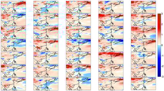
Figure 1.
Summer SAT trends [1966–2005; °C (40 yr)−1] over East Asia derived from the CESM1 ensemble members (35). The subplot in the top-left corner represents member 1, counting forward towards the right.
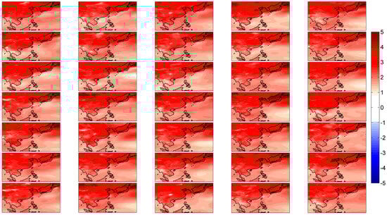
Figure 2.
Summer SAT trends [2010–2060; °C (51 yr)−1] over East Asia derived from the CESM1 ensemble members (35). The subplot in the top-left corner represents member 1, counting forward towards the right.
In Figure 2, the projected summer mean SAT trends under the RCP 8.5 scenario display a warming trend in most places of the East Asian region, unequivocally in all of the 35 ensemble members. However, the magnitude of warming differs among the runs, e.g., poleward amplification (≥4 °C) trend throughout Northern China is predominant in some of the members (EM 4, 12, 19, 20, 28, 29 and 32), while EM 2, 8, 10, 13, 14, 16, 17, 18, 23, 30 and 33 display a strong east–west contrast in warming magnitudes (<3 °C). Additionally, a weak warming trend throughout the East Asian region is prominent in a few of the ensemble members (6, 7, 11, 22, 24, 25, 26 and 31).
In addition, CRU-based station observation datasets exhibit strong decadal variability in SAT during the summer monsoon months. The linear trend during 1966–2005 is plotted in Figure 3, which displays a strong cooling trend in the northern (above 35° N) and southern parts (below 25° N), whereas the central part (between 25° and 35° N) of the East Asian region has experienced a strong warming trend. The cooling trend in the northern part can be seen in EM 4, 14, 16, 18, 19, 22 and 25, while the cooling trend in the southern part is prominent in EM 7, 12, 14, 20, 24 and 29. On the contrary, in the central part of East Asia, the warming trend is consistent in EM 11 and 15. Therefore, we can infer that, over East Asia, the CESM model can nicely replicate the observed summer temperature trends, and the warming amplitudes are comparable during the analyzed period.
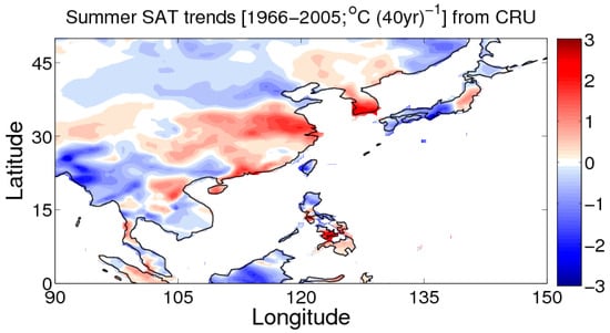
Figure 3.
Summer SAT trends [1966–2005; °C (40 yr)−1] over East Asia derived from the CRU-based observation data.
3.2. Partitioning of Total Trends into External Forcing Factors and Internal Variability
We partitioned the total trends into the contributions of external forcings and internal variability (Equation (1)). The spatial pattern of the ensemble mean trend (significance > 95%) is displayed in the upper and lower panels of Figure 4 for the historical and RCP8.5 scenarios, respectively. The ensemble mean trend of the 35 member ensembles illustrates a continental-scale warming pattern over East Asia, which attains a maximum value that exceeds 2 °C. There is a strong spatial disparity in the regional warming pattern: the amplitude is lowest in the central part, while in the poleward side, the warming trend (~1.5 °C) displays a contiguous pattern stretching throughout the northern part of East Asia (above 35° N). Like the upper panel, the lower panel (i.e., under the RCP8.5 scenario) exhibits an identical warming trend, albeit the magnitude is much higher throughout the East Asian region (~2.5 °C).
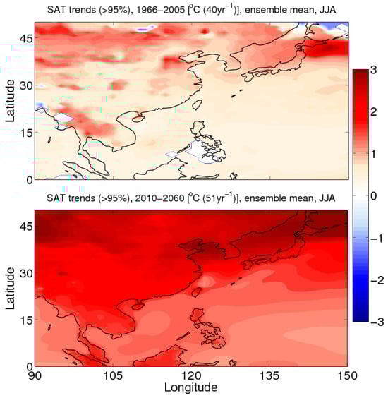
Figure 4.
Ensemble mean SAT trends over East Asia for the historical [1966–2005; °C (40 yr)−1] (top panel) and RCP8.5 [2010–2060; °C (51 yr)−1] (bottom panel) scenarios.
Figure 5 and Figure 6 display the internal variability during the historical and the RCP8.5 scenarios, respectively. A careful investigation of Figure 5 reveals a strong cooling trend in EM 14, 16, 18 and 19, while a warming trend appears to dominate in EM 9, 15, 17, 24 and 28, particularly in the northern part of the East Asian region. Moreover, some of the members (EM 1, 3, 12 and 20) display a strong east–west contrast in the warming and cooling trend, while the pattern flips for EM 6, 8 and 33. In Figure 6, most of the members display a cooling trend under the RCP8.5 scenario; however, EM 4, 17, 19, 28, 29, 30 and 32 exhibit a strong warming trend in the northern part of East Asia. Internal variability, therefore, incorporates a wide range of uncertainties into the model.
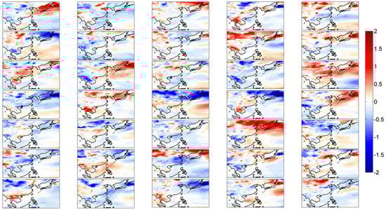
Figure 5.
Internal variability over East Asia, derived by subtracting the summer mean SAT trend over East Asia from the total trends [1966–2005; °C (40 yr)−1]. The top-left panel represents ensemble member 1.
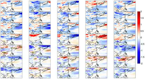
Figure 6.
Internal variability over East Asia, derived by subtracting the summer mean SAT trend over East Asia from the total trends [2010–2060; °C (51 yr)−1]. The top-left panel represents ensemble member 1.
Let us consider two member ensembles during the historical periods, e.g., 18 and 24, which represent the runs that possess the least and strongest warming trends, respectively, over East Asia. The characteristics of the trends (Figure 1) are markedly different between the two members: run 18 shows a strong cooling trend in the northern part (<−2.5 °C) of East Asia and is coupled with a weak warming trend (<1.5 °C) below 35° N; on the other hand, run 24 shows a pattern of a strong warming trend (>2 °C) that stretches over an extended landmass across the northern part of East Asia (above 35° N), while a diffuse warming pattern stretches southwards across the wider swath of the East Asian region. In the northern part of East Asia, the magnitude of warming differs widely between the two runs, which is primarily due to the differences in internal variability. Unlike the historical scenario, total trends in the RCP8.5 scenario are mostly dominated by external forcings, while natural variability in EM 2, 22, 25 and 31 displays a strong decline that counteracts the future warming trend to a certain extent.
3.3. Signal-to-Noise Ratio
In the above sections, we illustrate the methodology to partition the total trends into contributions from external forcing factors and internal variability. The results provide an impression on the amplitudes and patterns of SAT over East Asia under the historical and RCP8.5 scenarios. Here, we employ the Signal-to-Noise Ratio (SNR) analysis to assess the relative strength of both factors (Equation (3)). Figure 4 illustrates the contribution due to external forcings, while Figure 7a,b display the standard deviation of all the trends as a measure of internal variability for historical and future scenarios, respectively. From Figure 7, we can infer that internal variability introduces a wide range of uncertainty over East Asia, particularly in the northern (above 35° N) and southwestern parts (15–25° N and 90–105° E). As evident from Figure 7, internal variability decreases significantly in South China (e.g., Yunnan province), Myanmar, Vietnam, Cambodia and Thailand in the future, while the features remain more or less the same in other parts of East Asia.
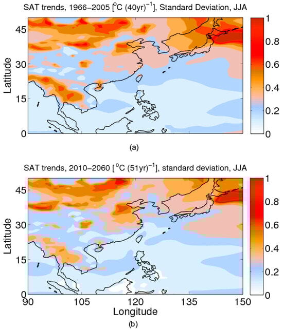
Figure 7.
Standard deviation of the SAT trends over East Asia for the historical period (a) and standard deviation of the SAT trends over East Asia under the RCP8.5 scenario (b). The higher the standard deviation, the higher is the contribution of internal variability.
Figure 8a,b show the SNR for the historical and RCP8.5 scenarios, respectively. During the historical period, the SNR is less than 1 over most of the East Asian landmass, and the values are relatively higher (~1–3) in the west-central part of China. This indicates that, in the historical period, internal variability in the SAT trend dominates over the forced responses. In contrast, under the RCP8.5 scenario (bottom panel), the SNR is higher than 4, and in some places (Yangtze River basin), it reaches 15, which indicates that external factors maximally contribute to the future SAT trend and internal variability has a minimum contribution over East Asia.
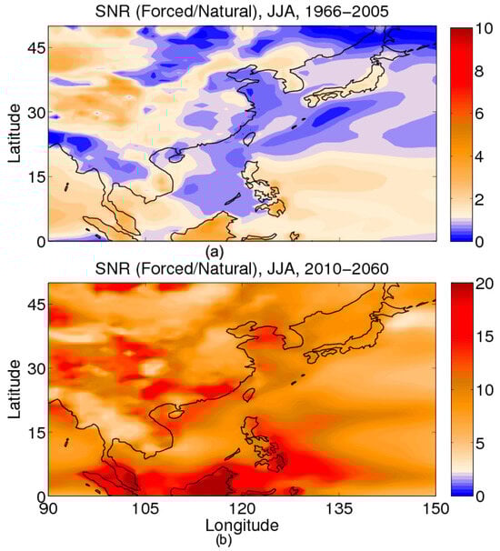
Figure 8.
SNR over East Asia during the 1966–2005 period (a) and SNR over East Asia during the 2010–2060 period (b). SNR < 1 means internal variability overrides external forcing factors.
3.4. Chances of Warming/Cooling Trends
Large ensemble simulations are suitable for calculating the chances or probability of warming or cooling during the historical and the RCP8.5 scenarios. The chances of warming can be counted as the percentage of occurrences of simulations that are exhibiting a positive/warming trend with respect to the total number of simulations (Equation (4)). The occurrence of a trend with an opposite sign may arise due to variabilities that are intrinsic to the climate system. The chances of positive SAT trends under the historical (1966–2005) and RCP8.5 scenarios (2010–2060) are shown in the upper and bottom panels of Figure 9, respectively.
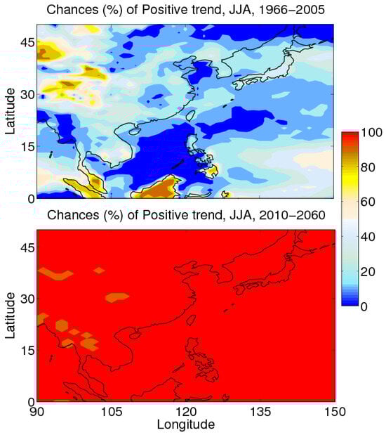
Figure 9.
Percentage of occurrences or chances of a warming/positive trend over East Asia during the 1966–2005 period (top panel) and 2010–2060 period (bottom panel). Note that the lower the chances of warming, the higher are the chances of cooling.
The chances of the summer season cooling over East Asia are higher than 80% in the CESM1 model simulations. The cooling trend is stronger in the northern and southwestern parts of East Asia and over the South China Sea as well, while in the west-central part of East Asia, the chances of warming vary within 60–90%. It is noteworthy that the lower the chances of warming (positive trend), the higher are the chances of cooling (negative trend). In contrast, the chances of warming over all of East Asia touch 100% under the RCP8.5 scenario.
3.5. Percentage Contribution of External Forcings and Internal Variability over East Asia
Here, we estimate the relative contribution (%) of external forcing factors and internal variability on SAT within the spatial domain of 15–45° N and 100–140° E. The area averaged mean SAT of the 35 member ensembles and their standard deviations are plotted in Figure 10a as a black line and gray vertical shading, respectively. Until the late 1990s, the mean SAT anomalies vary between −0.15 °C and 0.2 °C, whereas it increases from ~0.3 °C in 2000 to ~4.3 °C in 2075. The magenta line represents the area averaged SAT anomaly from the CRU-based observation data, which is used to validate the model output results. The observed timeseries reflects the SAT variability that combines the contributions from external forcing factors and overlying internal variability. The interannual variability of the observed timeseries navigates well within the lower and upper bound of the standard deviation, which confirms the reliability of the model outputs in simulating the East Asian climate. In addition, the timeseries of the SNR is used to quantify the relative roles of external and internal factors that are influencing the SAT trends over East Asia. The blue and red shadings indicate that the SNR is <1 until 2000, while in the post-2000 period, the SNR is >1 and reaches ~15 in 2075, respectively. It indicates that, before 2000, internal variability dominates external forcings, while after 2000, external forcings override internal variability. To extract the low-frequency signals, we employed a running mean filter of 11 years on each of the variables to smooth out the interannual variability.
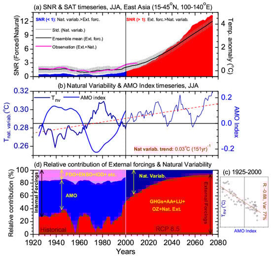
Figure 10.
(a) Ensemble mean SAT anomaly timeseries (black line) and standard deviation (gray vertical lines) are shown in the right axis. The magenta line indicates the CRU-based observation data. The red and blue shadings indicate SNR > 1 and SNR < 1, respectively. (b) Left axis indicates Tnatural variability (deep blue line; standard deviation), and right axis indicates AMO index (light blue). The red dotted line represents the linear trend in Tnatural variability. (c) Corr. Coeff. between AMO index and Tnatural variability. (d) The red and blue shadings represent percentage contribution of external forcing factors and internal variability. We applied an 11-year smoothing filter to suppress the interannual variability.
Here, we estimate the relative contribution (%) of external forcing factors and internal variability on SAT within the spatial domain of 15–45° N and 100–140° E. The area averaged mean SAT of the 35 member ensembles and their standard deviations are plotted in Figure 10a as a black line and gray vertical shading, respectively. Until the late 1990s, the mean SAT anomalies vary between −0.15 °C and 0.2 °C, whereas it increases from ~0.3 °C in 2000 to ~4.3 °C in 2075. The magenta line represents the area averaged SAT anomaly from the CRU-based observation data, which is used to validate the model output results. The observed timeseries reflects the SAT variability that combines the contributions from external forcing factors and overlying internal variability. The interannual variability of the observed timeseries navigates well within the lower and upper bound of the standard deviation, which confirms the reliability of the model outputs in simulating the East Asian climate. The significant (>95%) correlation coefficient, mean bias and root mean square error (RMSE) between the model SAT and CRU-based SAT are 0.92, 0.06455 and 0.1153, respectively.
In addition, the timeseries of the SNR is used to quantify the relative roles of external and internal factors that are influencing the SAT trends over East Asia. The blue and red shadings indicate that the SNR is <1 until 2000, while in the post-2000 period, the SNR is >1 and reaches ~15 in 2075, respectively. It indicates that, before 2000, internal variability dominates external forcings, while after 2000, external forcings override internal variability. To extract the low-frequency signals, we employed a running mean filter of 11 years on each of the variables to smooth out the interannual variability. Figure 11 represents the timeseries of the SNR with 95% confidence limits.
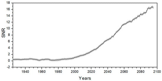
Figure 11.
Timeseries of SNR with 95% confidence limits.
In the next step, we analyze the physical factors that are underlying the changes in SAT variability until 2000. To do this, it is essential to investigate the dynamical mechanisms that drive the intrinsic variability within the atmospheric circulation system. Changes in atmospheric circulation may alter the SAT by means of moisture flux transport and advection of heat from distant sources (e.g., Atlantic sources). Previous studies have shown that the Atlantic Multidecadal Oscillation (AMO) in its negative phase accounts for ~55% of the total variance that explains the multidecadal variability over the Central Indian landmasses in the latter half of the twentieth century []. In the negative phase of the AMO, strong signals of Rossby waves are emanating from the North Atlantic Ocean and propagate across the Eurasian continent, which affects SAT variability through teleconnection. Here, in this section, we try to establish the empirical relationship between summer mean SAT variability over East Asia and the AMO.
The timeseries of internal variability (Tnv, i.e., standard deviation) from 1925 to 2075 (deep blue line; left panel) and the Atlantic Multidecadal Oscillation (AMO) index from 1925 to 2000 (light blue line; right panel), respectively, are plotted in Figure 10b. Between 1928 and 1962 and after 1997, the AMO is in the positive phase, while before 1928 and between 1963 and 1996, the phase of the AMO is negative. To examine the long-term tendency in Tnv, we perform a trend analysis (red dotted line) between 1925 and 2075, which displays an increasing SAT variability (0.03 °C/yr). The AMO in its negative phase contributes more to the SAT variability, and it experiences a multidecadal shift around the mid-1960s—a period that coincides exactly with the AMO phase shift. To further confirm the covariability, we perform a correlation analysis between the timeseries of Tnv and the AMO index during 1925 and 2000 (Figure 10c). The correlation coefficient is −0.88, which accounts for ~77% of the variances that explain the SAT variability during the analyzed period (1925–2000). It indicates that, before 2000, the AMO maximally contributes (~75–80%) to the internal variability over East Asia, which has not been reported before.
As evident from Nath et al., (2019) [], the Rossby wave train that is emanating from the North Atlantic Ocean in the negative phase of the AMO develops a strong teleconnection pattern across Eurasia towards Central India [] and East Asia. Like the Central Indian landmasses, this wave train of North Atlantic origin is also responsible for the SAT variabilities in East Asia. Figure 10d illustrates the relative contribution (%, Equation (5)) of external forcing factors and internal variability on the historical and projected trends of SAT over East Asia. Until 2000, external forcings (anthropogenic + external natural) contribute no more than 20–30% (red area) of the SAT variability, whereas natural variability (AMO + PDO + ENSO + IOD, etc.) strongly overrides the total trend (70–80%). As mentioned above, the AMO is the largest contributor (~50–60%); and PDO, ENSO, IOD, etc. share the rest (~15%) of the SAT variability during summer (Figure 12). Of them, IOD contributes ~11%, while the ENSO and PDO have non-significant contributions to the SAT variability. However, after 2000, natural variability exhibits a slow increasing trend until the end of the 21st century under the RCP8.5 scenario, the contribution due to external forcings increases rapidly from ~55% in 2000 to ~95% in 2075, and natural variability has a minimum contribution to the SAT variability over East Asia. In the next section, we investigate the role of albedo feedback on the increasing role of external forcings that drive the SAT trend in the post-2000 period.
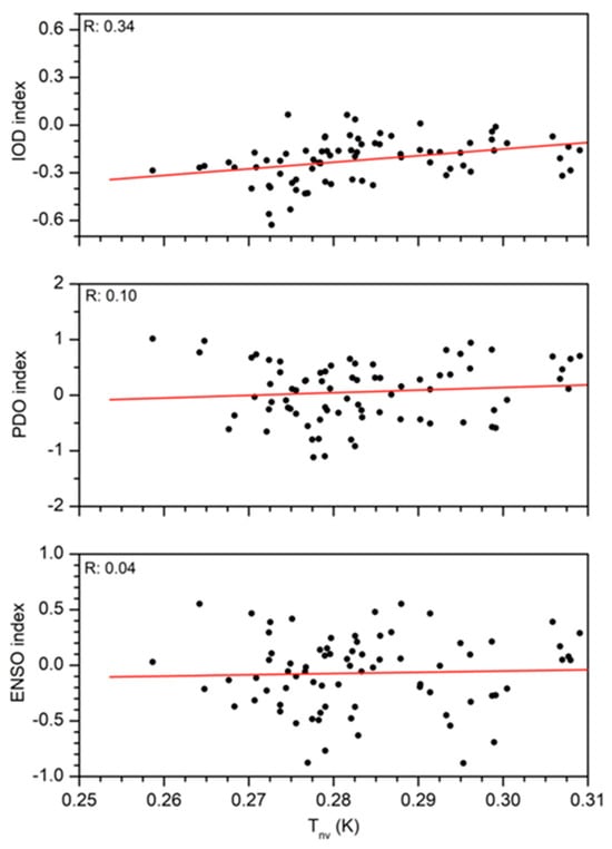
Figure 12.
Correlation analysis between Tnatural variability and IOD index (top panel), between Tnatural variability and PDO index (middle panel) and between Tnatural variability and ENSO index (bottom panel).
3.6. Increasing SAT Variability and Albedo Feedback
In the tropics, albedo feedback significantly affects the energy balance and surface temperature rise through several interrelated mechanisms, e.g., a decrease in albedo indicates that less solar radiation is reflected back into space and more is absorbed by the Earth’s surface. This increased absorption could disrupt the local climate systems and contribute to a greater surface temperature rise due to strong changes in albedo feedback. In the tropical regions, where sunlight is abundant, even a small decrease in albedo can result in a substantial increase in absorbed solar energy, thereby raising the local temperatures. In East Asia, the timeseries of albedo (mean + standard deviation) increases until 2000, and then it stabilizes until 2010; thereafter, it decreases significantly, which is consistent with the monotonic increase in ensemble mean SAT until the end of the 21st century (Figure 13). It indicates that, under the RCP8.5 scenario, albedo feedback has a strong impact on external forcings, which increases the surface warming by overriding the contribution of internal variability in the future.
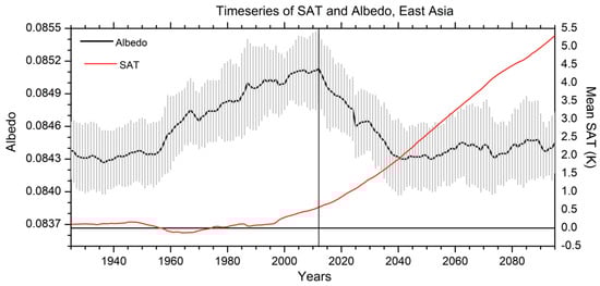
Figure 13.
Timeseries of ensemble mean SAT (red line) and timeseries of ensemble mean albedo (black line) and its standard deviation (gray shading) over East Asia.
The decrease in albedo under the RCP8.5 scenario is the consequence of more solar energy being trapped by the surface and less radiation being reflected back to the atmosphere. In addition, a lower albedo often results in more solar energy being absorbed by the Earth system at the top of the atmosphere and thereby contributing to the warming by altering the energy balance dynamics. Therefore, it is imperative to understand this relationship for predicting the future changes in global temperatures over East Asia. In Figure 14, we plotted the timeseries of downward solar flux anomalies (red line) and net solar flux anomalies (black line) at the surface and at the top of the atmosphere, respectively. Initially, the fluxes had decreased until 2010, and thereafter, they increase until the end of the 21st century, which is consistent with the increasing and decreasing trends in SAT and albedo, respectively.
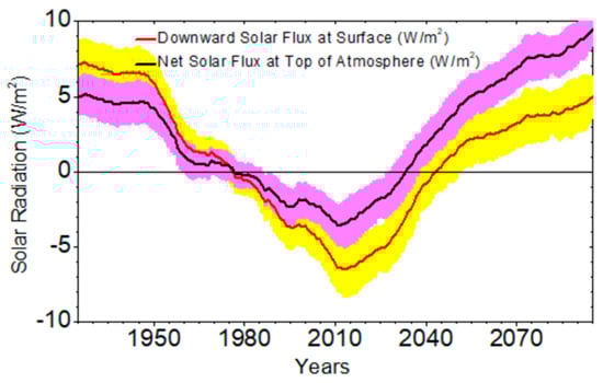
Figure 14.
Timeseries of ensemble mean downward solar flux anomalies at the surface (red line) and its standard deviation (yellow shading) and timeseries of ensemble mean net solar flux at the top of the atmosphere (black line) and its standard deviation (magenta shading) over East Asia.
As incoming solar radiation flux increases at the surface, albedo decreases, and the additional heat is transferred to the atmosphere above. This increases the sensible heat fluxes over East Asia by transferring the heat from the Earth’s surface to the atmosphere due to a greater temperature gradient between the ground and the atmosphere. This heterogeneity results in differential heating, causing the changes in the local temperatures over East Asia. To ascertain these changes, the timeseries of sensible heat flux anomaly is plotted in Figure 15, which displays an increasing trend that is consistent with the increasing trend in ensemble mean SAT over East Asia. Therefore, in the post-2010 period, more incoming solar radiation fluxes are trapped by the surface, causing the albedo to decrease and the sensible heat flux to increase rapidly. It contributes significantly to external forcings in driving the SAT under the RCP8.5 scenario.
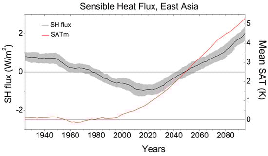
Figure 15.
Timeseries of SAT (red line) and timeseries of ensemble mean sensible heat flux (black line) and its standard deviation (gray shading) over East Asia.
The empirical relationships between the downward solar fluxes at the surface and sensible heat flux and between sensible heat flux and SAT anomalies are established by computing the correlation coefficients between the variables in Figure 16. The correlation coefficient between the downward solar flux anomaly at the surface and sensible heat flux anomaly is 0.94 and between sensible heat flux and SAT anomaly is 0.99. They account for ~88% and ~98% of the variances that explain the multidecadal changes in ensemble mean SAT under the RCP8.5 scenario, respectively.
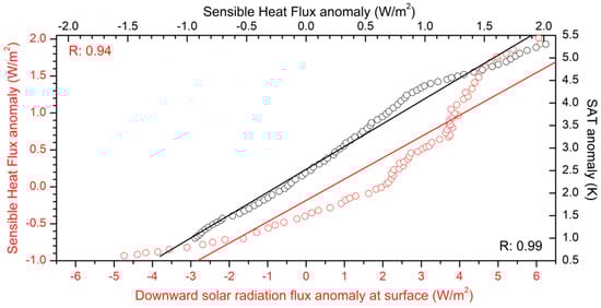
Figure 16.
Correlation coefficient between downward solar radiation flux anomalies at the surface and sensible heat flux anomaly (bottom-left) and correlation coefficient between SAT anomaly and sensible heat flux anomaly (top-right) over East Asia.
4. Summary and Discussion
In the present manuscript, the historical and near-term changes (1920–2080) in SAT over East Asia are assessed using the CESM-LE simulations. Since individual runs of the member ensembles are forced with identical external forcing with slight differences in their initial atmospheric condition, internal variability introduces a wide range of uncertainty or spread in the model projections. We partitioned the total trends into contributions from external forcings and internal variability, which can be measured as the mean and standard deviation of 35 member ensembles. In the historical period, seasonal mean (JJA) SAT trends over East Asia exhibit a wide range of diversity, with strong cooling (≤−2 °C) and warming (≥2 °C) trends among the members. On the other hand, under the RCP8.5 scenario, the East Asian region is mostly dominated by a warming trend (≥4 °C). In the historical period, the contribution from external forcings to the total warming trend is weaker, while the warming trend amplifies multifold (~1.5–2.5 °C) under the RCP8.5 scenario, particularly in the northern part of East Asia. Both for the historical and RCP8.5 scenarios, the ensemble members differ widely in terms of sign and magnitude of warming over East Asia, which is primarily due to the internal variability.
Here, we used the SNR as a metric to quantify the relative contribution of external forcings and internal variability to the SAT trend over East Asia. In the historical period, internal variability dominates over external forcings (SNR < 1), while external forcing overrides internal variability (SNR > 4) under the RCP8.5 scenario. In the historical period, the chances of East Asia cooling are higher than 80%, while the chances of warming touch ~100% under the RCP8.5 scenario. Therefore, the cooling trend due to internal variability partially counteracted the warming trend due to external forcing factors. The novel aspects of the current manuscript include the following. The cooling trend is more pronounced during the negative phase of the AMO, i.e., between the mid-1960s and 2000, which accounts for ~70–80% of the total SAT variability of East Asia. In the negative phase of the AMO, Rossby wave trains of North Atlantic origin may influence the cooling trend over East Asia. Secondly, after 2000, external forcing exhibits a slow but continuous increasing trend from ~55% in 2000 to 95% in 2075. Finally, we investigate the role of albedo feedback and increasing contribution of sensible heat fluxes in driving the warming trend under the RCP8.5 scenario. Here, we observe that the increasing trend in ensemble mean SAT is driven by the decreasing trend in albedo due to trapping of more downward heat fluxes in the future. It will increase the sensible heat fluxes over East Asia due to a greater temperature gradient between the ground and the atmosphere. This differential heating will increase the local temperatures and strongly override internal variability under the RCP8.5 scenario.
After 2000, due to large shifts in chances and magnitude of warming, the rates of climate change over East Asia are much higher than the historical mean trend. However, the impact of extreme climate change on East Asian monsoon and circulation is still unclear. The natural systems, which are sensitive to climate-related changes at larger timescales, are undergoing changes at unprecedented rates. It is anticipated that, in the following decades to come, the rate of climate change and its impacts will intensify further in magnitude and extent. Therefore, detection, attribution and adaptation to these changes will be sustained for decades to come, even under effective emission mitigation efforts. Mitigation measures to combat emissions and limit the magnitude and duration of changes at higher rates and longer timescales would be needed urgently.
Author Contributions
R.N. and D.N. designed the concept and methodological process of this study. R.N. carried out the main data analysis, with support from D.N. R.N. downloaded and provided the data and associated variables for this study. D.N. wrote the manuscript. W.C. provided valuable guidance for interpreting the results and revised the draft. All authors discussed the results, provided comments during the preparation of the manuscript. All authors have read and agreed to the published version of the manuscript.
Funding
This research was funded by the Yunnan Provincial Science and Technology Department Funding (Grant Nos. 202505AB350001 and 202503AP140009).
Institutional Review Board Statement
Not applicable.
Informed Consent Statement
Not applicable.
Data Availability Statement
The data that support the findings of this study are available from https://www.earthsystemgrid.org/dataset/ucar.cgd.ccsm4.cesmLE.lnd.proc.monthly_ave.html (accessed on 16 July 2017). The details are available in Hurrell et al., 2013 [] and Deser et al., 2014 []. The codes related to this analysis are available from the corresponding authors.
Acknowledgments
The research work is supported by The Yunnan Provincial Science and Technology Department.
Conflicts of Interest
The authors declare no conflict of interest.
References
- Deser, C.; Phillips, A.S.; Alexander, M.A.; Smoliak, B.V. Projecting North American Climate over the Next 50 Years: Uncertainty due to Internal Variability. J. Clim. 2014, 27, 2271–2296. [Google Scholar] [CrossRef]
- Deser, C.; Knutti, R.; Solomon, S.; Phillips, A.S. Communication of the role of natural variability in future North American climate. Nat. Clim. Chang. 2012, 2, 775–779. [Google Scholar] [CrossRef]
- Santer, B.D.; Mears, C.; Doutriaux, C.; Caldwell, P.; Gleckler, P.J.; Wigley, T.M.L.; Solomon, S.; Gillett, N.P.; Ivanova, D.; Karl, T.R.; et al. Separating signal and noise in atmospheric temperature changes: The importance of timescale. J. Geophys. Res. 2011, 116, D22105. [Google Scholar] [CrossRef]
- Meehl, G.A.; Hu, A.; Arblaster, J.M.; Fasullo, J.; Trenberth, K.E. Externally forced and internally generated decadal climate variability associated with the interdecadal Pacific oscillation. J. Clim. 2013, 26, 7298–7310. [Google Scholar] [CrossRef]
- Deser, C.; Phillips, A.S.; Bourdette, V.; Teng, H. Uncertainty in climate change projections: The role of internal variability. Clim. Dyn. 2012, 38, 527–546. [Google Scholar] [CrossRef]
- Wallace, J.M.; Deser, C.; Smoliak, B.V. Attribution of climate change in the presence of internal variability. In Climate Change: Multidecadal and Beyond; Chang, C.P., Ghil, M., Latif, M., Wallace, J.M., Eds.; Asia-Pacific Weather and Climate Series; World Scientific: Hackensack, NJ, USA, 2014; Volume 6. [Google Scholar]
- Hawkins, E.; Sutton, R. The potential to narrow uncertainty in regional climate predictions. Bull. Am. Meteorol. Soc. 2009, 90, 1095–1107. [Google Scholar] [CrossRef]
- Intergovernmental Panel on Climate Change (IPCC). Climate Change 2014: Synthesis Report; Fifth Assessment Report; Intergovernmental Panel on Climate Change (IPCC): Geneva, Switzerland, 2014; pp. 35–143. [Google Scholar]
- Tebaldi, C.; Arblaster, J.M.; Knutti, R. Mapping model agreement on future climate projections. Geophys. Res. Lett. 2011, 38, L23701. [Google Scholar] [CrossRef]
- Lei, Y.; Hoskins, B.; Slingo, J. Exploring the interplay between natural decadal variability and anthropogenic climate change in summer rainfall over China. Part I: Observational evidence. J. Clim. 2011, 24, 4584–4599. [Google Scholar] [CrossRef]
- Yu, R.; Wang, B.; Zhou, T. Tropospheric cooling and summer monsoon weakening trend over East Asia. Geophys. Res. Lett. 2004, 31, L22212. [Google Scholar] [CrossRef]
- Yu, R.; Zhou, T. Seasonality and three-dimensional structure of the interdecadal change in East Asian monsoon. J. Clim. 2007, 20, 5344–5355. [Google Scholar] [CrossRef]
- Huangfu, J.; Huang, R.H.; Chen, W. Influence of Tropical Western Pacific Warm Pool Thermal State on the Interdecadal Change of the Onset of the South China Sea Summer Monsoon in the Late-1990s. Atmos. Ocean. Sci. Lett. 2015, 8, 95–99. [Google Scholar] [CrossRef]
- Hansen, J.; Sato, M.; Ruedy, R. Perception of Climate Change. Proc. Natl. Acad. Sci. USA 2012, 109, 14726–14727. [Google Scholar] [CrossRef]
- Nath, R.; Luo, Y. Disentangling the influencing factors driving the cooling trend in boreal summer over Indo-Gangetic river basin, India: Role of Atlantic multidecadal oscillation (AMO). Theor. App. Clim. 2019, 138, 1–12. [Google Scholar] [CrossRef]
- Ueda, H.; Iwai, A.; Kuwako, K.; Hori, M.E. Impact of anthropogenic forcing on the Asian summer monsoon as simulated by eight GCMs. Geophys. Res. Lett. 2006, 33, L06703. [Google Scholar] [CrossRef]
- Sun, Y.; Zhang, X.; Zwiers, F.W.; Song, L.; Wan, H.; Hu, T.; Yin, H.; Ren, G. Rapid increase in the risk of extreme summer heat in Eastern China. Nat. Clim. Change 2014, 4, 1082–1085. [Google Scholar] [CrossRef]
- Zhou, T.; Gong, D.; Li, B. Detecting and understanding the multi-decadal variability of the East Asian Summer Monsoon–Recent progress and state of affairs. Meteorol. Z. 2009, 18, 455–467. [Google Scholar] [CrossRef]
- Liu, J.; Chen, H. Albedo Changes and Their Effects on Regional Climate: A Case Study of East Asia. Clim. Dyn. 2023, 60, 345–360. [Google Scholar]
- Kim, S.; Lee, D. Sensible Heat Flux Variability and Its Impact on Urban Climate in East Asian Cities. Urban Clim. 2023, 40, 100–115. [Google Scholar]
- Wang, Y.; Zhang, L. Impact of Urbanization on Surface Temperature Variability in East Asia. J. Clim. 2022, 35, 1234–1250. [Google Scholar]
- Solomon, S.; Qin, D.; Manning, M.; Chen, Z. Climate Change 2007: The Physical Science Basis; Cambridge University Press: Cambridge, UK, 2007; p. 996. [Google Scholar]
- Hurrell, J.W.; Holland, M.M.; Gent, P.R.; Ghan, S.; Kay, J.; Kushner, P.; Lamarque, J.-F.; Large, W.G.; Lawrence, D.M.; Lindsay, K.; et al. The Community Earth System Model: A Framework for Collaborative Research. Bull. Am. Meteorol. Soc. 2013, 94, 1339–1360. [Google Scholar] [CrossRef]
- Lorenz, E.N. Deterministic non periodic flow. J. Atmos. Sci. 1963, 20, 130–141. [Google Scholar] [CrossRef]
- Nath, R.; Luo, Y. On the contribution of internal variability and external forcing factors to the Cooling trend over the Humid Subtropical Indo-Gangetic Plain in India. Sci. Rep. 2018, 8, 18047. [Google Scholar] [CrossRef] [PubMed]
- Lamarque, J.-F.; Kyle, G.P.; Meinshausen, M.; Riahi, K.; Smith, S.J.; van Vuuren, D.P.; Conley, A.J.; Vitt, F. Global and regional evolution of short-lived radiatively-active gases and aerosols in the representative concentration pathways. Clim. Change 2011, 109, 191–212. [Google Scholar] [CrossRef]
- Meinshausen, M.; Smith, S.J.; Calvin, K.; Daniel, J.S.; Kainuma, M.L.T.; Lamarque, J.-F.; Matsumoto, K.; Montzka, S.A.; Raper, S.C.B.; Riahi, K.; et al. The RCP greenhouse gas concentrations and their extension from 1765 to 2300. Clim. Change 2011, 109, 213–241. [Google Scholar] [CrossRef]
- Newman, M.; Alexander, M.A.; Ault, T.R.; Cobb, K.M.; Deser, C.; Di Lorenzo, E.; Mantua, N.; Miller, A.J.; Minobe, S.; Nakamura, H.; et al. The Pacific Decadal Oscillation, Revisited. J. Clim. 2016, 29, 4399–4427. [Google Scholar] [CrossRef]
- Rayner, N.A.; Parker, D.E.; Horton, E.B.; Folland, C.K.; Alexander, L.V.; Rowell, D.P.; Kent, E.C.; Kaplan, A. Global analyses of sea surface temperature, sea ice, and night marine air temperature since the late nineteenth century. J. Geophys. Res. 2003, 108, 4407. [Google Scholar] [CrossRef]
- Saji, N.H.; Yamagata, T. Structure of SST and Surface Wind Variability during Indian Ocean Dipole Mode Events: COADS Observations. J. Clim. 2003, 16, 2735–2751. [Google Scholar] [CrossRef]
Disclaimer/Publisher’s Note: The statements, opinions and data contained in all publications are solely those of the individual author(s) and contributor(s) and not of MDPI and/or the editor(s). MDPI and/or the editor(s) disclaim responsibility for any injury to people or property resulting from any ideas, methods, instructions or products referred to in the content. |
© 2025 by the authors. Licensee MDPI, Basel, Switzerland. This article is an open access article distributed under the terms and conditions of the Creative Commons Attribution (CC BY) license (https://creativecommons.org/licenses/by/4.0/).