Characteristics of Rain and Sea Spray Droplet Size Distribution at a Marine Tower

Abstract

The effects of sea spray on open-ocean rainfall measurements-the drop size distribution (DSD) and rainfall intensities-were studied using a state-of-the-art optical disdrometer. The number of rain droplets less than 1 mm in diameter is affected by several factors, including the type of rainfall and seasonality. Over the ocean, small rain and large sea spray droplets co-exist in the same diameter size class (0.072 to 1000 mm); hence, sea spray creates uncertainty when seeking to characterize the drop size distribution (DSD) of rain droplets over the ocean. We measured droplet sizes at a marine tower using a state-of-the-art optical disdrometer, a tipping-bucket rain gauge, a wind anemometer, and a time-lapse camera, over a period that included typhoon Krosa of 2019. The number of rain droplets of diameter less than 1 mm increased monotonically as the horizontal wind speed became stronger. Thus, the shape parameter μ of the Ulbrich distribution decreased. This decreasing trend can be recognized as an increase in sea spray. During no-rainfall hours (indicated by rain gauges on the ocean tower and nearby land), sea spray DSDs were obtained at various horizontal wind speeds. Furthermore, the proportions of sea spray to rainfall at different rainfall intensities and horizontal wind speeds were determined; at a horizontal wind speed of 16 to 20 m s⁻¹, the average sea spray proportions were 82.7%, 19.1%, and 5.3% during total rainfall periods of 2.1 mm h⁻¹, 8.9 mm h⁻¹, and 32.1 mm h⁻¹, respectively. Representation of sea spray DSDs, as well as rainfall DSDs, is a key element of calculating real rainfall intensities over the open ocean.

1. Introduction

Rainfall measurement over the open ocean plays a leading role in validating satellite precipitation and global climate models e.g., [1,2,3,4]. During storms, rainfall intensities measured by tipping-bucket rain gauges over the open ocean (e.g., on ships) are addressed by both rain droplets and sea spray e.g., [5]. Remarkably, sea spray exists even on land; during severe typhoons (e.g., Trami of 2018, associated with a maximum instantaneous wind speed of 42 m s⁻¹ at Choshi in the Kanto region of Japan), tiny droplets of sea spray were blown to Tsukuba city even located 50 km from the Pacific coast, resulting in salt damage [6]. Notably, sea spray exerts influence on momentum, latent, and sensible heat fluxes within the context of air-sea interactions [7,8,9], and rain droplets play an indispensable role in flux exchanges [10,11].

Small rain and large sea spray droplets co-exist in the diameter class of less than 1 mm, and this has made distinguishing them difficult in practice. To estimate the proportion of sea spray to total rainfall, salinity measurements of water collected in a rain gauge were performed [5]; yet, this observation underlined the limitation of rain containing dissolved dry salt (reviewed in [1]). Thereby, the gauge was placed at least 16 m above the water level, so that the proportion of sea spray was minimized (reviewed in [1]).

In order to distinguish between sea spray and rain droplets, the characteristics of rainfall intensity and the numbers of rain droplets of various diameters-the drop size distribution (DSD) need to be analyzed. DSD is used in conjunction with multi-doppler polarization systems to estimate rainfall intensity from radar reflectivity data, using the Z–R relationship for weak rainfall and the K_dp–R relationship for heavy rainfall [12]. It highlights the correlations between rain intensity and Z, (radar reflectivity), as well as between rain intensity and K_dp (specific differential phase shift of radar). The first and most well-known DSD model, the Marshall–Palmer distribution [13], was derived from observations of rain droplets of diameter 0.1 to 5 mm spreading on dyed filter papers. Later, other equations were developed to characterize DSD denoted by log-normal, Weibull, exponential, and gamma and general gamma distributions. The latter usefully describes the drizzle mode and distributional tail of large droplets [14,15,16]. Among them, the Ulbrich distribution [17] is known as a special case of the general gamma distribution, and has been widely used to analyze rainfall, as it allows for DSD flexibility when the diameters are less than 1 mm. At certain rainfall intensities, the numbers of droplets less than 1 mm in diameter vary significantly compared to that of larger droplets. Such variations reflect the type of rainfall and the seasonality e.g., [18,19,20,21]. The DSD of Ulbrich [17] features a shape parameter μ, and for open-ocean rainfall measurement μ indicates the probability that the DSD variation of small-diameter droplets is affected by sea spray.

The Ulbrich distribution is expressed as:

$$N\left(D\right)=N_0{D}^{\mu }\exp \left(-\Lambda D\right)$$

(1)

where N(D) is the number of droplets in diameter D (cm), N₀ is 8 × 10⁴ m⁻³ cm^−1−μ, and μ (non-dimensional) and Λ (cm⁻¹) are shape parameters. Λ varies by the rainfall intensity R (mm h⁻¹), and is therefore assigned to Λ = 41 × R^−0.21. These two parameters N₀ and Λ are selected from [13]. When μ = 0, the equation is equivalent to the Marshall–Palmer distribution. Previous studies recorded variations in the diameter range as well as seasonal changes in the DSD shape parameters μ and Λ, where μ varied from −0.85 to 76.9 (although it was generally positive) and Λ ranged from 3.3 to 591.5 cm⁻¹ [18]. As μ varied from −1 through 0 to 1,we proposed two cases to investigate the proportion of small droplets (0.072 to 1.000 mm; this range corresponds to the detection limit of disdrometer) with respect to the total rainfall intensity. Firstly, as the total rainfall intensity reached 10 mm h⁻¹, the proportions of small droplets became 72%, 17%, and 2%, determined by Equation (1). Likewise, as the total rainfall intensity reached 50 mm h⁻¹ the proportions of small droplets became 40%, 6%, and 0.8%. The results revealed that light rainfall intensity was dominated by small droplets. Sea spray observation over the open ocean was first described in [22]. Several studies have highlighted the significance of sea spray generation at air-sea interface by investigating rainfall effect on its generation [23,24]; yet, these results show the contradictory results. Sea spray is thought to be generated predominantly by rainfall [23], while the others note that heavy rainfall can act to suppress significant wave height [24], suggesting the suppression of sea spray generation by rainfall. Moreover, wet and dry deposition and scavenging efficiency can be influenced by rain and sea spray [25]. Following this line of research, not only the effect of rainfall but whitecap formation time, decay time [26], as well as sea state [27], may have an impact on the generation of sea spray. Sea water temperature could be a key element according to the laboratory experiments showing that high temperatures led to the low production of sea spray [28]. In addition, a new observation system proposed in [29] provides an overview of the relationship between surface-generation noise and sea spray aerosols. These findings may open the way to better understand the potential role of sea spray in air–sea interaction, but details of these studies are beyond the scope of our study.

Sea spray generally has three types of droplets: film droplets (0.00001 mm~0.1 mm), jet droplets (0.001~0.1 mm), and spume droplets (0.01~1 mm) [30]. Here, we focus on spume droplets, although this size class of 0.072 to 1.000 mm is exceptional in [23]. Compared to the other types of droplets, spume droplets facilitate a greater transfer of heat and moisture across the air-sea interface in a rapid manner. A wind speed over about 7–11 m s⁻¹ is typically required to generate the droplets [31], which are ripped off wave crests by wind, principally via the bag-breakup fragmentation first described in [32]. The DSDs of sea spray have been extensively studied [31,33,34] while one review considered the DSDs of spume droplets (Figure 6 of cited article [31]) at a wind speed of 15 m s⁻¹. From the Figure, the number of spume droplets spans two orders of magnitude. The review paper [31] introduces three types of DSDs of spume droplets [35,36,37]. One of them was proposed by observational data, and the others were by results obtained from the theoretical analysis and wind-tunnel experiment, although all publications mentioned that there was still a lack of data describing DSDs of spume droplets.

The diameter of rain droplets ranges from approximately 0.1 to 5 mm, and that of large sea spray droplets from 0.01 to 1 mm. Thus, in the diameter range below 1 mm, both droplets co-exist. Here, we performed a series of observations using a state-of-the-art disdrometer at a marine tower off the coast of Wakayama Prefecture in Japan (see Figure 1). The observational period ran from August to October in 2019, including a day during which a typhoon passed nearby. The proportions of sea spray to total rainfall measured by a tipping-bucket rain gauge were used to derive sea spray DSDs as a function of horizontal wind speeds. In Section 2, our observations, the use of disdrometer, and the data correction methodology, are described. The results of our observations are available and discussed in Section 3, and our findings are analyzed in Section 4.

2. Methods

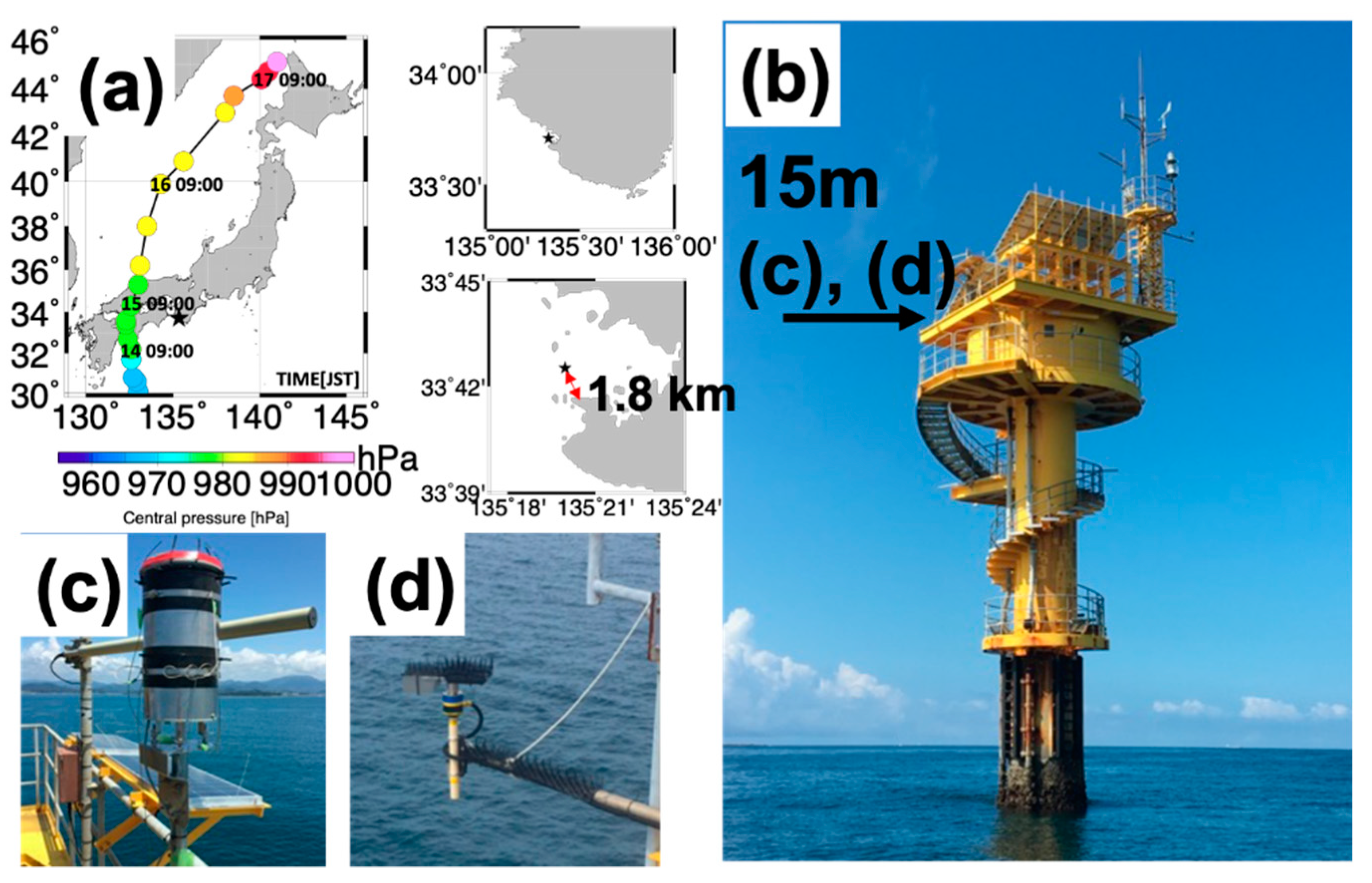
2.1. Site and Data Collection

A series of observations were conducted using a disdrometer called SPC (Niigata Electric; [38]), anemometer, time-lapse camera, and tipping-bucket rain gauge installed on an observational tower maintained by the Disaster Prevention Research Institute of Kyoto University (33°42′32″ N, 135°19′58″ E) at a vertical height of 15 m above sea level (Figure 1a). This height is higher than the one set in [23], so we do not consider the increase of sea spray generation by rainfall. The tower lies 1.8 km off the coast (see the two-headed arrow of Figure 1a). All wind speed and rainfall measurements were validated based on the data obtained from an automated meteorological data acquisition system (AMeDAS) weather station, which was located 4 km south of the tower and maintained by the Japan Meteorological Agency [39]. This station was equipped with a tipping-bucket rain gauge with resolution, 0.5 mm h⁻¹. We conducted continuous observations during two rainfall events, from 14 to 16 August and 17 to 19 October in 2019. These periods included the extreme event of Typhoon Krosa, and the typhoon track and central pressure are shown in Figure 1a.

2.2. Disdrometer

A disdrometer was firstly used to detect snow particles [40]. The disdrometer used in this study was thus modified by Niigata Electric [38] to detect water droplets with both vertical and horizontal trajectories based on the reviewed paper [41]. With reference to the conventional approach, a small tungsten lamp with a hood emits light in one arm, and then another arm with two phototransistors is fixed on the same optical axis, where snow particles pass through the area between the emitter and the receiver; in the meantime, the phototransistors output signals reflecting particle sizes on the assumption that the particle is in a spherical form [38]. This allows the disdrometer to detect not only snow [42,43], but also sand [44] and water droplets on the upper deck of an icebreaker [45,46]. However, this underestimates snow particle numbers by 20% compared to a fabric trap [47]. Thus, the disdrometer we used featured a self-steering wind vane with a super-luminescent diode sensor to enable stable output signals. Each signal is classified into 1 of 64 diameter classes between 0.072 and 1 mm every second, to deduce the size of particle passing through the sampling area (3 × 25 × 1 mm).

To calibrate the disdrometer, thin wires with different diameters were passed vertically through the sampling area in accordance with the previous study [48]. The calibration pointed out the error of measurement related to diameter sizes $\mp 15\mathsf{\mu }\mathrm{m}$ but to the number of droplets, which was not reported in previous studies [42,43,44,45,46]. In addition, the raw data contained systematic errors, due to ambient temperature and detector lens pollution by dust; yet water particles, including rain and sea spray, were successfully detected. The maximum and minimum threshold droplet numbers to 1000 s⁻¹ and 10 h⁻¹ were set, and thereafter the DSD was calculated as follows:

$$N\left(D_i\right)=\frac{n\left(D_i\right)}{A\times \mathsf{\Delta }t\times v\left(D_i\right)\times \mathsf{\Delta }{D}_i}$$

(2)

where n(D_i) represents the number of raindrops in diameter class i, D_i the mean of the diameter class i, A the sampling area of the particle counter surface (=0.000025 m²), $\mathsf{\Delta }t$ the sampling time (=3600 s), v(D_i) the terminal fall velocity of rain with diameter, and $\mathsf{\Delta }$D_i the diameter interval between the two successive classes, i and i + 1. Following this calculation, the rainfall intensity contributed by small droplets (hereafter, R_SPC) was determined.

2.3. Data Correction for Tipping Bucket

Errors associated with the rainfall measurements included wetting loss, evaporation, splashing of water into and out of the rain gauge, and wind-induced undercatch. Undercatch occurs due to deformation of the local wind field by the rain gauge, resulting in changes in raindrop trajectory; the effect of this phenomenon (examined by comparing reference gauges-installed in pits to minimize wind deformation—with above-ground gauges) is typically 2–10% [49]. The rain gauge data was adjusted using the commonly used empirical model [50] followed by the later modification [51], as shown below.

$$\begin{gathered} {\mathrm{R}}_{\mathrm{ctb}}=k\times {\mathrm{R}}_{\mathrm{tb}} \\ k=\exp \left[a-b\times \ln \left({\mathrm{R}}_{\mathrm{tb}}\right)-c\times u\times \ln \left({\mathrm{R}}_{\mathrm{tb}}\right)+d\times u\right] \end{gathered}$$

(3)

where a = −0.042303, b = 0.00101, c = 0.018177, and d = 0.043931 are empirical parameters [51] and R_tb, R_ctb, and u are the rainfall intensity yielded by the rain gauge, the corrected rainfall intensity, and the horizontal wind speed, respectively. This method is conventionally used to reduce the wind-induced effect.

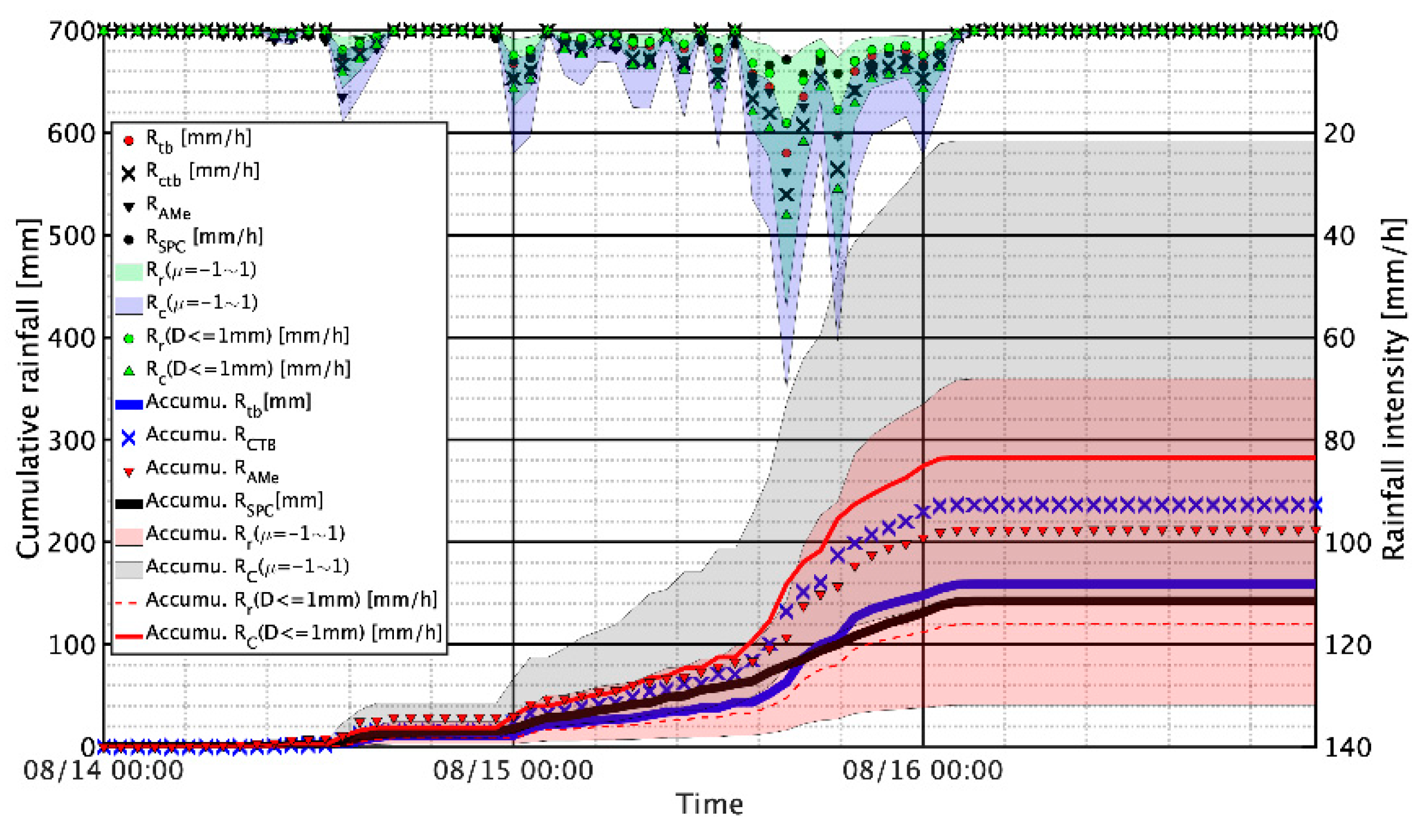
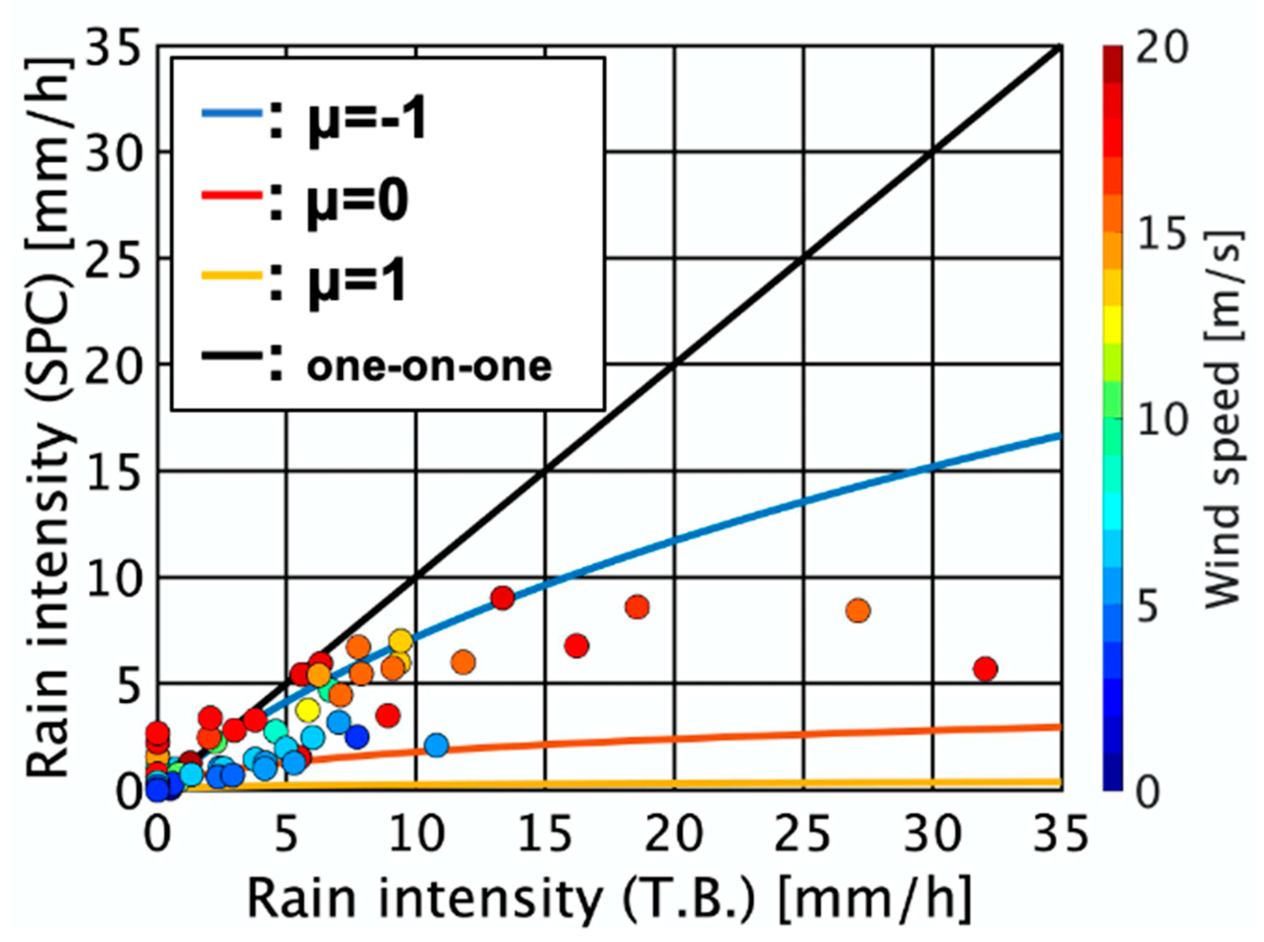
2.4. Estimation Methods

We first calculated the rainfall intensity of small droplets (diameter, 0.072–1.000 mm) using the empirical function of Equation (1) and compared it to the R_SPC. In this analysis, the parameters of Equation (1) were set to N₀ = 8 × 10⁴ (m⁻³ cm^−1−μ) and Λ = 41 × R^−0.21. To calculate the parameter Λ (=41 × R^−0.21), R_tb and R_ctb were substituted into R. The results followed the (Rr(D < 1) and Rc(D < 1)) values of Figure 2 in which the shape parameter μ was set to −1 and 1. Here, (Rr(D < 1) and Rc(D < 1)) reflect the calculation results of rainfall intensity contributed by small droplets using different rainfall data sets (R_tb and R_ctb), respectively.

Our second analysis evaluated the properties of parameters, Λ and μ in Equation (1). μ was estimated using the least-squares method as shown in Figure 3. N₀ was set to 8 × 10⁴ (m⁻³ cm^−1−μ). Afterwards, a time series of the shape parameter from Equation (1) was obtained. The root mean squared error between this equation and the observation data was 7.4 × 10⁶. The root mean logarithmic error and the coefficient of determination were 77.4 and 0.63, respectively.

Furthermore, DSDs of rain and sea spray were calculated based on the collected disdrometer data. While Equation (2) was utilized to calculate DSD of rain, the following equation was used for the sea spray calculation.

$$F\left(D_i\right)=\frac{n\left(D_i\right)}{A\times \mathsf{\Delta }t\times \mathsf{\Delta }{D}_i}$$

(4)

the unit of this F(D_i) is m⁻² s⁻¹ cm⁻¹.

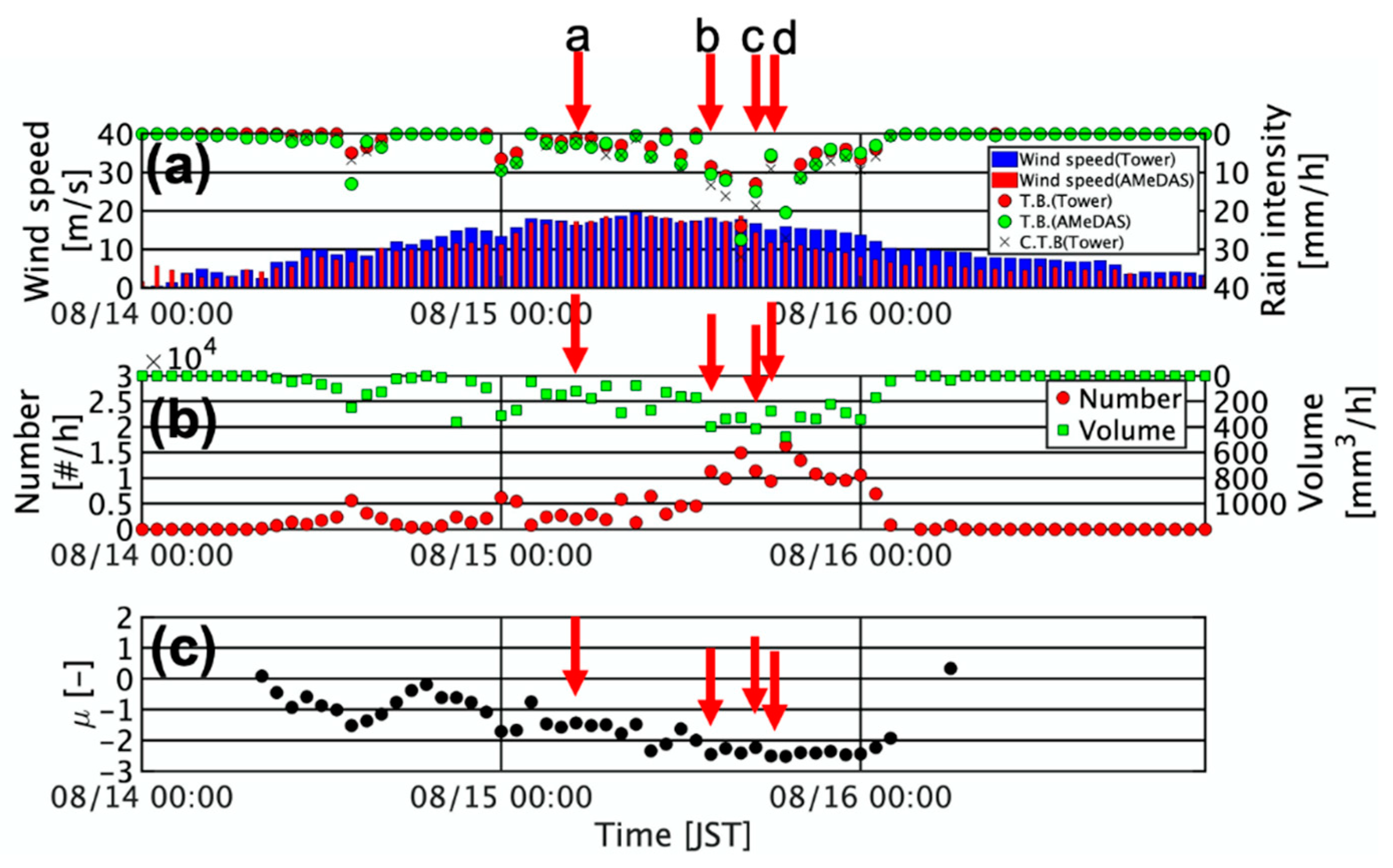
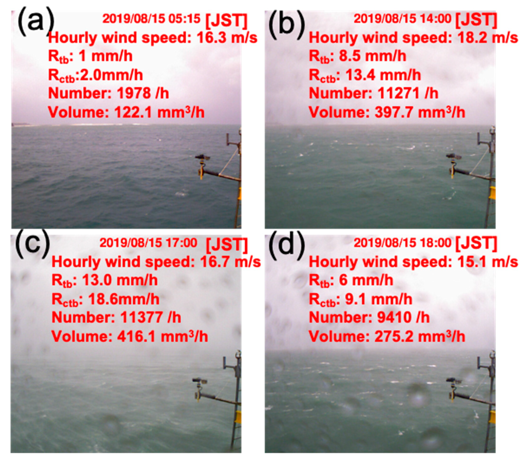
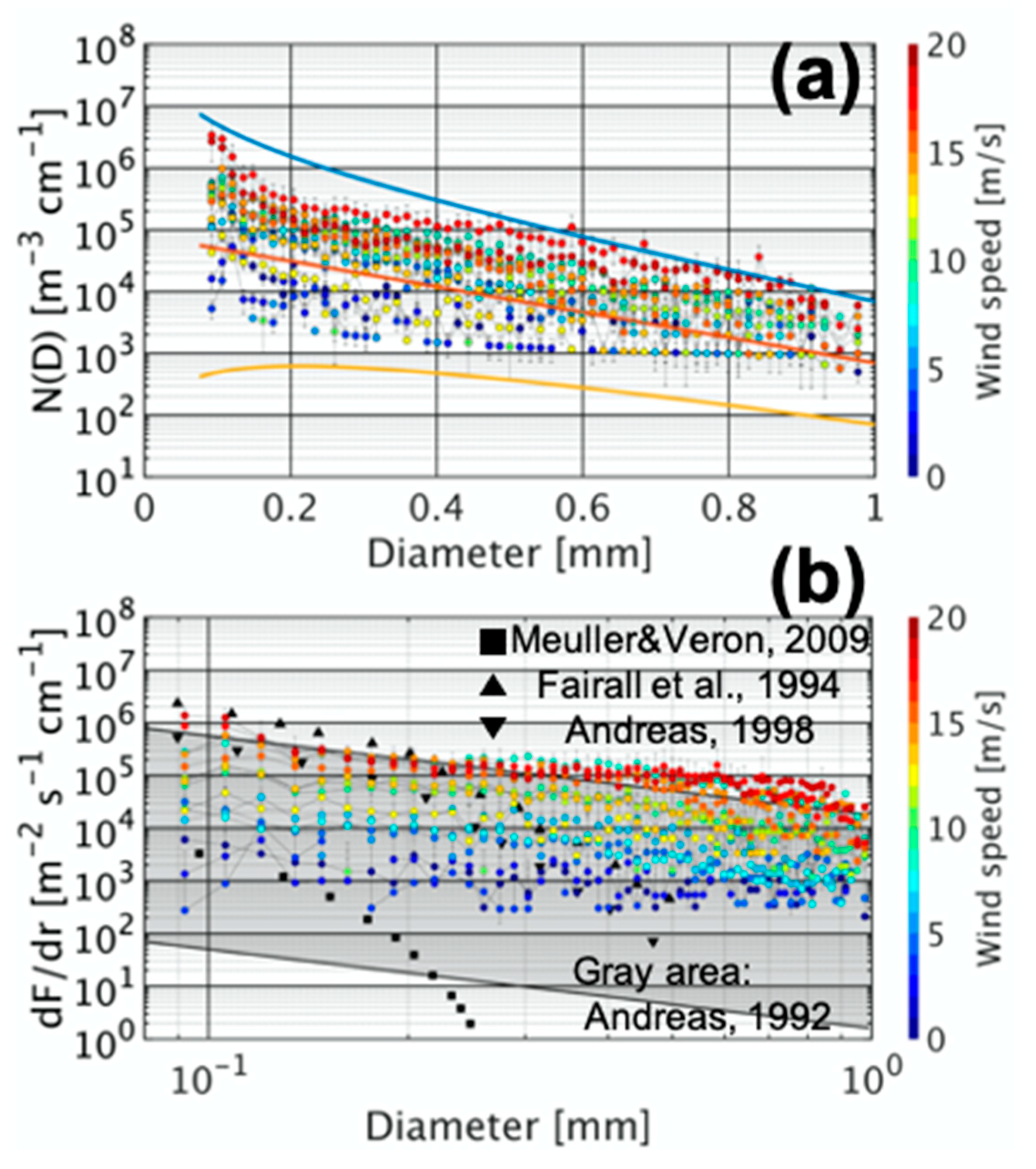
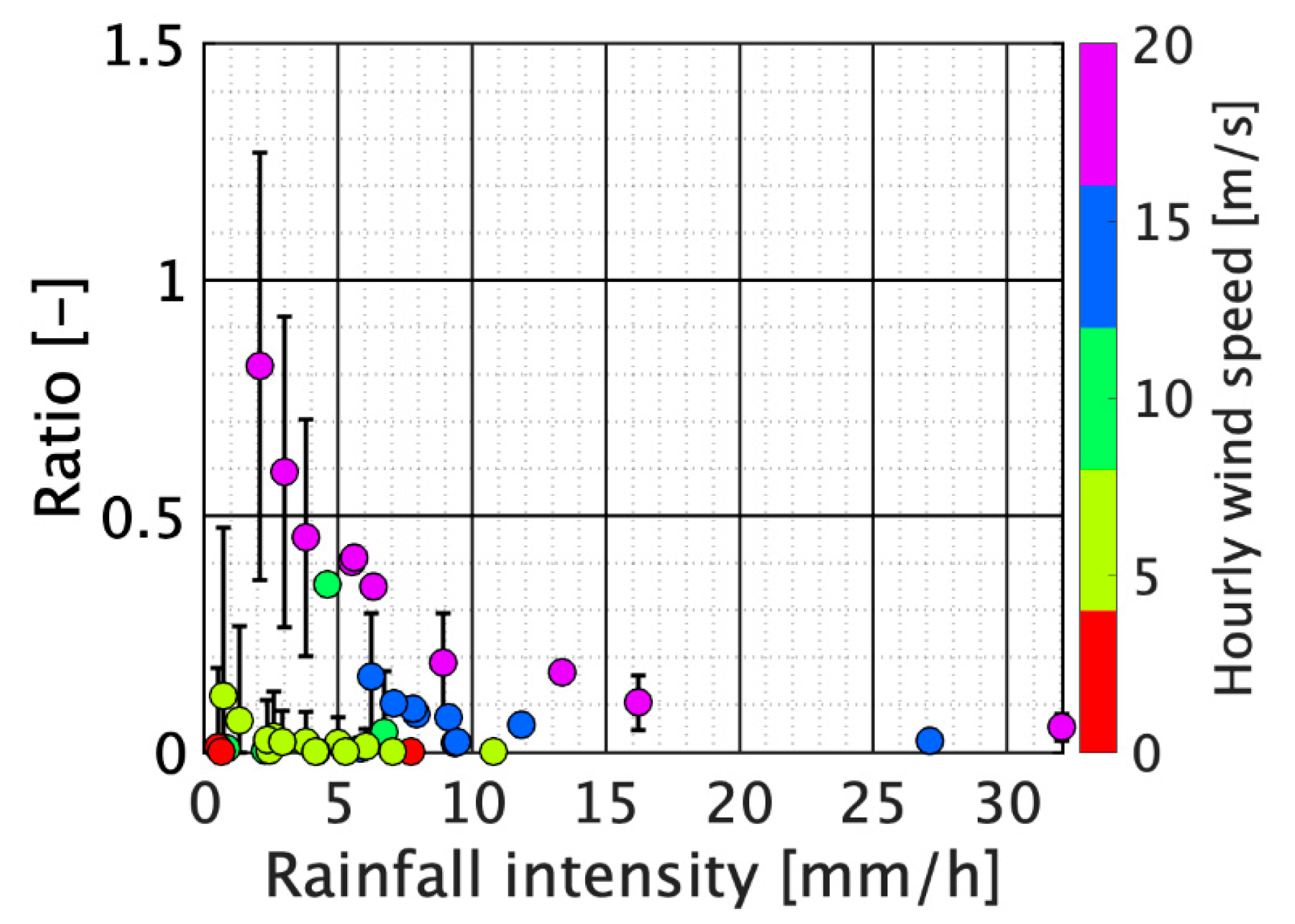
3. Results and Discussion

Experiments were accomplished using the disdrometer, which was designed to detect water droplets over the open ocean. The experimental design is visibly illustrated in Figure 1 (see Methods for more details). Time series data of rainfall intensity and cumulative rainfall were plotted based on the observations from 14 to 16 August in 2019 (JST) (Figure 2). The results showed that R_ctb was 1.32-fold greater than R_tb using the correction method, which tended to increase the R_ctb under strong windy and light rain. R_tb and R_ctb were 0.82- and 1.13-fold greater than the rainfall intensity detected at the AMeDAS station (R_AMe). The R_SPC followed the rises and falls in R_tb and R_ctb. The results of Rr(D < 1) and Rc(D < 1) mentioned in Section 2.4 are indicated by the blue and green areas. Compared to Rr(D < 1) and Rc(D < 1), R_SPC fell within the range of μ = −1 to 1. The green circles and triangles are Rr(D < 1) and Rc(D < 1) with the shape parameter μ = 0, which is equivalent to the Marshall–Palmer distribution. The left axis shows the cumulative rainfall for each component (R_tb, R_ctb, R_SPC, Rr(D < 1) and Rc(D < 1)) from 00:00 on 14 August (JST). During light rainfall at 13:00 (JST) on August 15, accumulative R_SPC recorded the cumulative R_tb and R_ctb. However, during heavy rain after 14:00 (JST) on August 15, the cumulative R_tb and R_ctb recorded drastic increases, leading to a large difference between the cumulative R_tb/ctb and cumulative R_SPC.

Figure 3a shows the time series of the hourly horizontal wind speed R_tb, R_ctb, and R_AMe, which are total rainfall measured by the tipping bucket at the tower and the AMeDAS station. Wind speed and rainfall intensity increased as the typhoon approached; however, wind speed at the AMeDAS station decreased earlier than did the wind speed at the tower, as the AMeDAS station was located further south. The rainfall intensity reached its peak when the wind speed decreased. In the meantime, the volume and total number of hourly droplets in the range of 0.072 to 1.000 mm in diameter were measured by the disdrometer at the tower, and both showed an increasing trend (Figure 3b). The shape parameter μ varied from −2.53 to 0.33 during this period, and decreased monotonically as the wind speed increased (Figure 3c). Although the rainfall decreased after 16:00 on August 15, μ continued to decrease during this period. Regarding the Ulbrich distribution, the numbers of small droplets less than 1 mm in diameter increased, while that of large droplets decreased.

Figure 4 shows the time-lapse photographs of the sea surface conditions at the time points indicated by the arrows in Figure 3a–d. In Figure 4a, R_tb and R_ctb were 1 and 2 mm h⁻¹, with 1978 droplets per hour and a volume of 122.1 mm³ h⁻¹, suggesting that the sea was calm. In Figure 4b, whitecaps were visible at a wind speed of 18.2 m s⁻¹ and the rainfall intensities (R_tb and R_ctb) were 8.5 mm h⁻¹ and 13.4 mm h⁻¹. In Figure 4c, the sea surface was covered with sea spray and streamlines were visible, assuming that droplets recorded by the disdrometer must have included sea spray. After the rainfall ended, some whitecaps remained (Figure 4d). From the time-lapse photographs, the disdrometer was not covered with waves, and the maximum significant height was 4.23 during the observation periods. The data sets were thus not influenced by waves directly.

Figure 2, Figure 3 and Figure 4 exhibited that rain and sea spray droplets less than 1 mm were detected by the disdrometer. To derive the proportions of small droplets against total rainfall, the relationships between R_ctb and R_SPC were drawn in Figure 5, in conjunction with the three lines based on the DSD of Equation (1). According to the data obtained from August to October, small droplets dominated the total rainfall during light rain. Nonetheless, the proportion was small during heavy rainfall. At wind speeds less than 5 m s⁻¹, the relationship followed the Marshall–Palmer distribution (red line), although R_SPC increased when R_ctb remained constant and the wind speed increased. Thus, the proportion of small droplets to total rainfall increased, reflecting the increasing amounts of sea spray as the horizontal wind speed increased. We hypothesize that the proportion of small droplets to total rainfall varies depending on the properties of sea spray. In the context of rain DSDs, this characteristic is important to estimate the real rainfall intensity, as the μ varies upon the amount of sea spray generated (Figure 5).

To investigate the proportion, DSDs of sea spray need to be discussed. Figure 6 shows the DSDs of rain and sea spray derived by the disdrometer during two periods—August and October, 2019—without rainfall monitored by the rain gauge. Even when the rain gauge revealed no rainfall, it was possible that rainfall may have been less than 0.5 mm h⁻¹, due to the resolution of the rain gauge. Usually, the DSD of rain is given in units of m⁻³ cm⁻¹_, and that of sea spray in units of m⁻² s⁻¹ cm⁻¹. The DSDs of rainfall below the resolution of the rain gauge and sea spray were averaged at the various wind speeds (from 1 to 20 m s⁻¹) at 1-m s⁻¹ intervals, in which the standard deviations derived (Figure 6a). The three DSD lines were derived from Equation (1) at rainfall of 0.5 mm h⁻¹ and μ values of −1, 0, and 1. All DSDs were within the range of the lines; however, to date it is difficult to define the causality of why the number of droplets increased with horizontal wind speed. In contrast, if the droplets were considered to be sea spray, the DSDs would be similar to the DSDs of sea spray reported previously for sea spray [33,35,36,37] (Figure 6b). Our findings were higher than the findings obtained at low wind speeds (up to 15 m s⁻¹), and presumably the DSDs from Figure 6a,b were DSDs of either rain or sea spray. Notably, the direct measurement of sea spray DSDs offers valuable data sets (Figure 6), as the direct approach has been rare in this field of study.

Finally, by means of the DSDs from Figure 6b, the proportions of sea spray to total rainfall (R_ctb) were highlighted in Figure 7. The DSD were identified at each wind speed, and the ratio of sea spray to R_ctb was calculated on the assumption that R_ctb contained both rain and sea spray. It suggests that sea spray occurs under high wind speeds. When the hourly wind speed varied from 16 to 20 m s⁻¹ (shown in purple dots in Figure 7), the average sea spray proportions were 82.7%, 19.1%, and 5.3%, with respect to the following rainfalls of 2.1 mm h⁻¹, 8.9 mm h⁻¹, and 32.1 mm h⁻¹, respectively. These results are similar to those expressed by the Ulbrich distribution in Section 1. Thus, variations in the numbers of small rain droplets (0.072 to 1.000 mm) are reflected by differences in the numbers of large sea spray droplets. Even at a strong rainfall intensity of 32 mm h⁻¹, the sea spray proportion remained at 5.3% at hourly horizontal wind speeds of 16 to 20 m s⁻¹. At horizontal wind speeds less than 12 m s⁻¹, the ratios were less than 10% regardless of the total rainfall. Moreover, the empirical equation for the decay curve ($y=a{\mathrm{e}}^{-b}$) was derived at the threshold hourly wind speeds of 5 m s⁻¹, 10 m s⁻¹, 15 m s⁻¹, and 20 m s⁻¹, respectively. The values of a and b in the decay curve (

Table 1. The parameters of the empirical equations yielding the proportions of sea spray at various rainfall intensities for different hourly wind speeds.

Hourly Wind Speed [m s−1]	a	b
0−5	4.05	−11.7
5−10	0.22	−0.89
10−15	0.050	0.16
15−20	0.16	−0.099

) are essential to estimate the rainfall intensity over the open ocean.

4. Summary

Understanding the sources and properties of small rain and large sea spray droplets common in the diameter class of less than 1 mm enables far more precise measurement of open-ocean rainfall (in this study, droplets with diameter of 0.072 to 1.000 mm was observed). We performed rain and sea spray observations at the marine tower using the disdrometer, rain gauge, anemometer, and time-lapse camera. The shape parameter μ of the Ulbrich distribution (as estimated by the disdrometer) decreased even after rainfall decreased, indicating an increase in the numbers of droplets less than 1 mm in diameter. Time-lapse images of the sea surface throughout the rain event showed large amounts of sea spray presenting as streamlines over the sea surface; it leads us to think that the disdrometer detects both rain and sea spray. The findings from our direct measurement may have important implications in the study of air-sea fluxes as only limited observational data are available at the moment.

Additionally, the relationship between the number of small droplets with diameters less than 1 mm and total rainfall intensity was investigated. As the wind grew stronger, the proportion of small droplets to total rainfall increased. This is because more sea spray is generated as the wind speed increases. What is more, DSDs were detected by the disdrometer during periods of rainfall less than 0.5 mm h⁻¹. Based on the results of previous studies, these DSDs could possibly be both rain and sea spray, though the higher DSDs correspond to the increased wind speed. Our final analysis revealed the proportion of sea spray to total rainfall, suggesting the contribution of sea spray to the rainfall measurement.

This study investigated the effects of sea spray on open-ocean rainfall measurements through the calculation of DSDs and rainfall intensities, based on the direct observational method. The study also explored the significance of spume droplet DSDs in estimating the air-sea fluxes of sensible and latent heat. In the context of rain DSDs, we proposed that the amount of sea spray generated could be another influential factor on possible variations of μ, in addition to the rainfall types and seasonality that were noted previously. Finally, the ratio of sea spray to the total rainfall was calculated to determine the contribution of sea spray, enabling us to improve the accuracy of rainfall estimates over the open ocean.

References

1. Yuter, S.E.; Parker, W.S. Rainfall measurement on ship revisited: The 1997 PACS TEPPS cruise. J. Appl. Meteorol. 2001, 40, 1003–1018. [Google Scholar] [CrossRef]
2. Yuter, S.E.; Houze, R.A., Jr. The 1997 pan American climate studies tropical Eastern Pacific process study. Part I: ITCZ region. Bull. Am. Meteorol. Soc. 2000, 81, 451–481. [Google Scholar] [CrossRef]
3. Bumke, K.; Fenning, K.; Strehz, A.; Mecking, R.; Schröder, M. HOAPS precipitation validation with ship-borne rain gauge measurements over the Baltic Sea. Tellus A Dyn. Meteorol. Oceanogr. 2012, 64, 18486. [Google Scholar] [CrossRef]
4. Hasse, L.; Grosskalaus, M.; Uhlig, K.; Timm, P. A ship rain gauge for use in high wind speeds. J. Atmos. Ocean. Technol. 1998, 15, 380–386. [Google Scholar] [CrossRef] [Green Version]
5. Skaar, J. On the measurement of precipitation at sea. Geophys. Publ. 1955, 19, 1–32. [Google Scholar]
6. Yamamoto, H.; Sakamoto, K.; Iwaya, K.; Kawamoto, E.; Nasu, M.; Watanabe, Y. Characteristics of meteorological and salt damage by Typhoon No.24 in 2018 (Trami). J. JSNDS 2019, 37, 365–382. (In Japanese) [Google Scholar]
7. Powell, M.D.; Vickery, P.J.; Reinhold, T.A. Reduced drag coefficient for high wind speeds in tropical cyclones. Nature 2003, 422, 279–283. [Google Scholar] [CrossRef]
8. Andreas, E.L. Spray stress revisited. J. Phys. Oceanogr. 2004, 34, 1429–1440. [Google Scholar] [CrossRef]
9. Andreas, E.L.; Mahrt, L.; Vickers, D. An improved bulk air–sea surface flux algorithm, including spray-mediated transfer. Quart. J. R. Meteor. Soc. 2015, 141, 642–654. [Google Scholar] [CrossRef]
10. Caldwell, D.R.; Elliot, W.P. Surface stresses produced by rainfall. J. Phys. Ocenogr. 1971, 1, 145–148. [Google Scholar] [CrossRef] [Green Version]
11. Caldwell, D.R.; Elliot, W.P. The effect of rainfall on the wind in the surface layer. Bound.-Layer Meteor. 1972, 3, 146–151. [Google Scholar] [CrossRef]
12. Doviak, R.; Zrnić, D.S. Doppler Radar and Weather Observations; Courier Corporation: North Chelmsford, MA, USA, 2006; pp. 219–235. [Google Scholar]
13. Marshall, J.S.; McK, P.W. The distribution of raindrops with size. J. Meteor. 1948, 5, 165–166. [Google Scholar] [CrossRef]
14. Auf der Maur, A.N. Statistical tools for drop size distribution: Moments and generalized gamma. J. Atmos. Sci. 2001, 58, 407–418. [Google Scholar] [CrossRef]
15. Lee, G.; Zawadzki, I.; Szyrmer, W.; Sempere-Torres, D.; Uijlenhoet, R. A general approach to double-moment normalization of drop size distributions. J. Appl. Meteorol. 2004, 43, 264–281. [Google Scholar] [CrossRef] [Green Version]
16. Thurai, M.; Bringi, V.N. Application of the generalized gamma model to represent the full rain drop size distribution spectra. J. Appl. Meteorol. Climatol. 2018, 57, 1197–1210. [Google Scholar] [CrossRef]
17. Ulbrich, C.W. Natural variation in the analytical form of the raindrop size distribution. J. Appl. Meteorol. 1983, 22, 1764–1775. [Google Scholar] [CrossRef] [Green Version]
18. Serio, M.A.; Carollo, F.G.; Ferro, V. Raindrop size distribution and terminal velocity for rainfall erosivity studies. A review. J. Hydrol. 2019, 276, 210–228. [Google Scholar] [CrossRef]
19. Adetan, O.; Afullo, T.J. Raindrop size distribution and rainfall attenuation modeling in equatorial and subtropical Africa: The critical diameters. Ann. Telecommun. 2014, 69, 607–619. [Google Scholar] [CrossRef]
20. Blanchard, D.C. Raindrop size-distribution in Hawaiian rains. J. Meteor. 1953, 10, 457–473. [Google Scholar] [CrossRef] [Green Version]
21. Hachani, S.; Boudevillain, B.; Delrieu, G.; Bargaoui, Z. Drop size distribution climatology in Cévennes-Vivarais region, France. Atmosphere 2017, 8, 233. [Google Scholar] [CrossRef] [Green Version]
22. Monahan, C.M. Sea spray as a function of low elevation wind speed. J. Geophys. Res. 1968, 73, 1127–1137. [Google Scholar] [CrossRef]
23. Marks, R. Preliminary investigations on the influence of rain on the production, concentration, and vertical distribution of sea salt aerosol. J. Geophys. Res. Oceans 1990, 95, 22299–22304. [Google Scholar] [CrossRef]
24. Cavaleri, L.; Bertotti, L.; Bidlot, J.-R. Waving in the rain. J. Geophys. Res. Oceans 2015, 120, 3248–3260. [Google Scholar] [CrossRef]
25. Lewis, E.R.; Schwartz, S.E. Sea Salt Aerosol Production Mechanisms, Methods, Measurements and Models, a Critical Review. Geophys. Monogr. 2004, 152, 71–74. [Google Scholar]
26. Callaghan, A.H. An improved whitecap timescale for sea spray aerosol production flux modeling using the discrete whitecap method. J. Geophys. Res. Atmos. 2013, 118, 9997–10010. [Google Scholar] [CrossRef]
27. Norris, S.J.; Brooks, I.M.; Hill, M.K.; Brooks, B.J.; Smith, M.H.; Sproson, D.A. Eddy covariance measurements of the sea spray aerosol flux over the open ocean. J. Geophys. Res. Atmos. 2012, 117, D07210. [Google Scholar] [CrossRef]
28. Salter, M.E.; Nilsson, E.D.; Butcher, A.; Bilde, M. On the seawater temperature dependence of the sea spray aerosol generated by a continuous plunging jet. J. Geophys. Res. Atmos. 2014, 119, 9052–9072. [Google Scholar] [CrossRef] [Green Version]
29. Markuszewski, P.; Klusek, Z.; Nilsson, E.D.; Petelski, T. Observations on relations between marine aerosol fluxes and surface-generated noise in the southern Baltic Sea. Oceanologia 2020, 62, 413–427. [Google Scholar] [CrossRef]
30. Veron, F. Ocean spray. Annu. Rev. Fluid Mech. 2015, 47, 507–538. [Google Scholar] [CrossRef]
31. Andreas, E.L. The temperature of evaporating sea spray droplets. J. Atmos. Sci. 1995, 52, 852–862. [Google Scholar] [CrossRef] [Green Version]
32. Gelfand, B.E. Droplet breakup phenomena in flows with velocity lag. Energy Combust. Sci. 1996, 22, 201. [Google Scholar] [CrossRef]
33. Andreas, E.L. Sea spray and the turbulent air-sea heat fluxes. J. Geophys. Res. 1992, 97, 11429–11441. [Google Scholar] [CrossRef]
34. Ortiz-Suslow, D.G.; Haus, B.K.; Mehta, S.; Laxague, N.J. Sea spray generation in very high winds. J. Atmos. Sci. 2016, 73, 3975–3995. [Google Scholar] [CrossRef]
35. Mueller, J.A.; Veron, F. A sea state–dependent spume generation function. J. Phys. Oceanogr. 2009, 39, 2363–2372. [Google Scholar] [CrossRef]
36. Fairall, C.W.; Kepert, J.D.; Holland, G.J. The effect of sea spray on surface energy transports over the ocean. Glob. Atmos. Ocean. Syst. 1994, 2, 121–142. [Google Scholar]
37. Andreas, E.L. A new sea spray generation function for wind speeds up to 32 m s−1. J. Phys. Oceanogr. 1998, 28, 2175–2184. [Google Scholar] [CrossRef] [Green Version]
38. Kimura, T.; Maruyama, T.; Ishimaru, T. SPC-III no sekkei to seisaku. Proc. Cold Reg. Technol. Conf. 1993, 665–670. (In Japanese) [Google Scholar]
39. Japan Meteorological Agency (JMA). Available online: http://www.jma.go.jp/en/amedas (accessed on 5 November 2020).
40. Schmidt, R.A. A system that measures blowing snow. USDA For. Serv. Res. Paper 1977, 194, 1–80. [Google Scholar]
41. Nishimura, K. Measurement of blowing snow. J. Fluid Mech. 2009, 28, 455–460. (In Japanese) [Google Scholar]
42. Sugiura, K.; Nishimura, K.; Maeno, N.; Kimura, T. Measurements of snow mass flux and transport rate at different particle diameters in drifting snow. Cold Reg. Sci. Technol. 1998, 27, 83–89. [Google Scholar] [CrossRef]
43. Sato, A. Calculation of size-effect of blowing snow particles on the snow particle counter (first report). Tech. Rep. Natl. Cent. Disaster Prev. 1987, 40, 93–101. [Google Scholar]
44. Mikami, M.; Yamada, Y.; Ishizuka, M.; Ishimaru, T.; Gao, W.; Zeng, F. Measurement of saltation process over Gobi and sand dunes in the Taklimakan desert, China, with newly developed sand particle counter. J. Geophys. Res. 2005, 110, D18S02. [Google Scholar] [CrossRef] [Green Version]
45. Ozeki, T.; Toda, S.; Yamaguchi, H. Field investigation of impinging seawater spray on the R/V Mirai using spray particle counter type sea spray meter. In Proceedings of the 33rd International Symposium on Okhotsk Sea and Polar Oceans, Hokkaido, Japan, 18–21 February 2018; Volume D-5, pp. 93–96. [Google Scholar]
46. Ozeki, T.; Shiga, T.; Sawamura, J.; Yashiro, Y.; Adachi, S.; Yamaguchi, H. Development of sea spray meters and an analysis of sea spray characteristics in large vessel. In Proceedings of the 26th International Ocean and Polar Engineering Conference, Rhodes, Greece, 26 June–1 July 2016; Volume 1, pp. 1335–1340. [Google Scholar]
47. Schmidt, R.A.; Meister, R.; Gubler, H. Comparison of snow drifting measurements at an alpine ridge crest. Cold Reg. Sci. Technol. 1984, 9, 131–141. [Google Scholar] [CrossRef]
48. Sato, T.; Kimura, T.; Ishimaru, T.; Maruyama, T. Field test of a new snow-particle counter (SPC) system. Ann. Glaciol. 1993, 18, 149–154. [Google Scholar] [CrossRef] [Green Version]
49. World Meteorological Organization. Guide to Hydrological Practices (WMO-No. 168); WMO: Geneva, Switzerland, 2008; Volume 1, pp. I.3–I.8. [Google Scholar]
50. World Meteorological Organization. Methods of Correction for Systematic Error in Point Precipitation Measurement for Operational Use; Operational Hydrology Report No. 21 (WO-No. 589); WMO: Genova, Switzerland, 1982. [Google Scholar]
51. Førland, E.J.; Hanssen-Bauer, I. Increased precipitation in the Norwegian Arctic: True or false? Clim. Chang. 2000, 46, 385–509. [Google Scholar] [CrossRef]
Figure 1. Map of the study area. (a) The observation site is indicated by black star. Colored circles indicate the central pressure and track of typhoon Krosa over time (JST). (b) The observational tower; the arrow indicates the height of the observation deck (15 m) and positions of the instruments, including (c) tipping bucket and (d) snow particle counter (SPC).
Atmosphere 11 01210 g001
Figure 2. Time series of rainfall intensity and cumulative rainfall from August 14 to 16 in 2019 (JST). Rainfall intensity (right axis) of Rtb and Rctb shown in red circles and black crosses, respectively. Rainfall intensity detected at the automated meteorological data acquisition system (AMeDAS) station (RAMe) is indicated in black triangles, and the intensity calculated from the SPC data (RSPC) is in black circles. The areas where the estimated results ((Rr(D < 1) and Rc(D < 1)) are described in Section 2.4, are highlighted in blue and green; they depend on the shape parameter (μ) values ranging from −1 to 1. The green circles and triangles represent Rr(D < 1) and Rc(D < 1) with μ = 0. Left vertical axis shows the cumulative rainfall for each component (Rtb, Rctb, RSPC, Rr(D < 1) and Rc(D < 1)) from 00:00 14 August (JST). Cumulative rainfall of Rtb and Rctb are shown in blue solid line and blue crosses, respectively, and that of RSPC is in black line. Cumulative rainfall of Rr(D < 1) and Rc(D < 1) with μ = 0 are expressed in red solid and dashed lines, respectively. Red area indicates the difference between the shape parameter μ = −1 and 1 where AMeDAS data points are plotted as red triangles.
Atmosphere 11 01210 g002
Figure 3. Time series of hourly wind speed and rainfall intensity (Rtb, Rctb, and RAMe), as well as the total number and volume of droplets and drop size distribution (DSD) shape parameter μ. (a) Wind speeds at the tower and AMeDAS station are expressed in blue and red bars, respectively. Rtb and Rctb are shown in green dots and black crosses, respectively, and RAMe is in red dots. (b) Red circles indicate the total number of droplets detected by the SPC. Green squares indicate total volume of particles. (c) DSD shape parameter μ is shown. Arrows in (a–d) indicate the time points photographed in Figure 4.
Atmosphere 11 01210 g003
Figure 4. (ad) Photographs of sea surface conditions at time points indicated by the arrows in Figure 3a–c.
Atmosphere 11 01210 g004
Figure 5. Relationship between rainfall intensity (Rctb) and the intensity derived from SPC data (RSPC). Hourly wind speed is indicated in bar colors. Lines indicate the relationship between rainfall intensity of drops with diameters less than 1 mm and total rainfall intensity based on Ulbrich distributions for different values of μ, where light blue = −1, red = 0, and orange = 1. Black line indicates a one-on-one line.
Atmosphere 11 01210 g005
Figure 6. DSDs that may include droplets derived from both rainfall and sea spray. Each DSD is averaged for each hourly wind speed. The black bars show standard deviation ( σ ). Bar colors indicate hourly wind speed. (a) Ulbrich distribution for different values of μ, where light blue = −1, red = 0, and orange = 1. (b) DSDs of sea spray at hourly wind speeds ranging from 1 to 20 m s−1 in intervals of 1 m s−1. The DSDs calculated in previous studies are also shown [33,35,36,37].
Atmosphere 11 01210 g006
Figure 7. Relationship between rainfall intensity of Rctb and ratio of sea spray against Rctb. Bar colors indicate hourly wind speed. Black bars indicate the maximum and minimum ranges.
Atmosphere 11 01210 g007