


Abstract
Ice adhesion on exposed structures remains a major operational challenge, motivating the search for passive, material-based anti-icing strategies. Molecular dynamics offers a controlled way to investigate ice–surface interactions beyond the limits of experimental setups. In this work, we develop a simulation framework to model the impact of solid hexagonal ice droplets on metallic substrates. Ice impacts are simulated across a range of velocities (10–120 m/s), temperatures (120–250 K), and face-centred cubic surface materials (gold, copper, silver, aluminum, and nickel). Using LAMMPS, mW water force-field, EAM/Alloy metal potentials, and Lennard-Jones water–surface interactions, we quantify phase evolution through angular order parameter and quasi-liquid layer measurements, complemented by the CHILL+ algorithm in OVITO. By isolating all external factors, we show that melting increases with velocity and temperature and correlates with substrate properties: metals with high thermal diffusivity and low Young’s modulus tend to decrease post-collision ice melting. The ratio of the former to the latter, a derived index of merit Υ, significantly correlates with melting percentage and identifies silver as the most effective anti-ice material examined. Statistical analyses strongly suggest that these surface properties influence interfacial melting, supporting the use of this modelling framework for screening and designing anti-icing materials.
1. Introduction
Ice adhesion to the surface of aircraft wings and fuselage is a crucial engineering issue in relation to the safety and efficiency of aviation [1,2]. Ice accumulation on these structures can not only create losses in aerodynamics and flight stability, but also cause major accidents [3,4]. This problem is not limited to aviation: other external structures can be affected [5]. In winter, solar panels and wind turbines see their productivity decrease due to ice accretion [6], a major problem that will become more frequent with the ongoing transition to alternative energy sources.
Current commercial de-icing strategies are predominantly centred on surface treatments using chemical fluids, with propylene glycol being among the most widely applied agents, especially in aviation [7]. Propylene glycol functions as a freezing-point depressant, lowering the temperature at which ice forms and enabling easier removal of ice and snow from surfaces [8,9]. However, despite it being considered less toxic than alternatives like ethylene glycol, its widespread use still poses environmental risks, as it flows into bodies of water and depletes their oxygen reserves, decreasing its bioavailability and affecting aquatic organisms [9,10]. In addition to these direct ecological impacts, the transportation and application of large quantities of de-icing fluids contribute further environmental costs through fuel use, emissions, and infrastructure [11].
Given these challenges, considerable effort has been directed toward the development of material-based icephobic surfaces aimed at preventing ice accretion or reducing ice adhesion. Studies on anti-ice surfaces have multiplied in recent years [12,13]; however, much of this work remains experimental and is often limited by the lack of access to atmospheric ice conditions for validation.
Computational-based studies have often relied on static simulations, testing ice adhesion strength once a water droplet has frozen on a surface [14,15,16,17,18]. These works essentially test the performance of superhydrophobic materials in facilitating ice removal by increasing the contact angle between the substrate and the water. As the contact angle determines surface wettability [19], the more hydrophobic a surface is, the less the adhesion strength is between it and newly formed ice [14]. Studying this phenomenon considers liquid water falling onto a static cold surface and freezing, a phenomenon that does occur often. However, some ice accretion occurs upon impact while an aircraft or wind turbine is moving and when the droplets are solid, such as in hailstorms. These hail events have become more common over the last few years with the rise in climate change-related effects, although the link between the two has not been entirely established [20]. In the United States, almost 7000 hail events have been reported in 2023 [21], while causing reportedly $14 billion in damages in 2020 [21]. This phenomenon thus deserves more attention, and we believe that modelling is the correct tool for this objective.
Experimental work employing atmospheric-type ice has been attempted, notably by using an ultrasonic levitator [22] and freezing water droplets with a cryogun placed above them, blowing cold air [23] until secondary nucleation occurs [24] and the droplet becomes solid. The levitator was then turned off, which allowed the droplet to be sped up by gravity until it hit a surface [25]. Several surfaces were tested, and the impact dynamics were analyzed with a high-speed camera [25].
Unfortunately, this experimental work has significant variability between experiments, as it is difficult to not only control the temperature of both the surface and the droplet, but also the environment surrounding the droplet during the drop and collision [26]. Gusts of wind, air currents, or instabilities in the levitator can introduce rotation, which is often invisible or hard to measure with a high-speed camera. Any changes in temperature or pressure can also provoke premature melting before the collision occurs [27], which severely impacts the results’ reproducibility. Finally, given the high-speed camera’s extremely limited focal plane paired with variation in rotation [28], it is challenging to obtain reproducible experimental results within a reasonable timeframe. As expected, rotation alters the downwards trajectory of the droplets, which pushes them out of the camera’s focal plane often. This effect is multiplied as the droplet height is increased, which severely limits the velocities that can be tested in experimental work, especially since the droplets can only be accelerated by gravity in a setup that is not immensely resource intensive [25].
Simulations can work with much higher, more realistic velocities than several previous physical studies [25,29], and give additional environmental controls that eliminate many experimental limitations. So far, dynamic impact-based simulation work has either strictly used subcooled water [30] or tested whether the ice droplets could cause plastic deformation on the surface [31]. While a significant proportion of ice accretion comes from subcooled liquid water freezing, hail impacts also tend to accumulate on surfaces, which is yet to be explored in modelling. In our work, we are interested in developing a system that can evaluate how well a surface prevents solid ice droplets from melting. This is useful since ice accretion typically occurs in the winter, the surface is usually cold, and melted ice tends to refreeze, which increases the surface area (and thus the adhesion strength) of ice, thus making it much harder to remove. A modelling-based framework capable of simulating ice–surface interactions across a range of materials, velocities, and temperatures could provide a cost-effective and streamlined approach for evaluating the anti-icing performance of potential surface compositions.
Previous computational and experimental studies have identified a crucial parameter that is important to consider in solid ice impacts on surface: the quasi-liquid layer (QLL) [32,33,34,35,36]. This pre-melted layer forms on the outside of a solid droplet and is the transition state between the ordered interior (hexagonal crystal) and the disordered exterior (liquid or gas) [37]. The thickness of this layer can be related to the bulk droplet temperature and can be used to relate experimental data with this modelling work, and by extension be part of the model validation.
The main objectives of this study are to (1) develop a molecular dynamics framework for simulating the impact of a solid hexagonal ice (ice Ih) droplet on metallic substrates; (2) determine the phase evolution of ice and quantify the energy transfer and temperature progression of the droplet during impact over velocities ranging from 10 to 120 m/s and system temperatures between 120 and 250 K on five different metal FCC surfaces; (3) statistically assess the impact of material properties on anti-ice performance and post-collision ice melting; and (4) experimentally validate the model.
The paper is organized as follows. We start by describing the computational techniques used to design the droplet–substrate system, with its associated force-fields. Then, we describe in depth the effect of temperature, velocity, and metal type on the droplet’s phase transition and energy balance before, during, and after collision. We then link the results from the materials tested to their mechanical and thermal properties by undergoing a statistical analysis and relating them to the literature data. Finally, we relate the model with experimental data through a morphological and droplet structure comparison and analysis of the quasi-liquid layer (QLL).
2. Materials and Methods
The LAMMPS (large-scale atomic/molecular massively parallel simulator, v. 1.12.0) [38,39] and Moltemplate (v. 2.22.5) [40] softwares are used for these simulations, with visualization being done with OVITO (v. 3.15.3) [41]. The boundary conditions in the x- and y-directions are shrink wrapped, while the z-direction employs fixed boundary conditions. Shrink wrap was chosen because it lets the lateral box dimensions adapt to the instantaneous particle positions, avoiding the computational requirements of semi-infinite periodic cells while permitting small adjustments in lateral stress [42]. This dynamic adjustment helps stabilize pressure in this solid–solid system, as the system is not constrained by strictly fixed boundaries. Its use in this type of system is also supported by the literature [30]. The simulation box dimensions are in the plane perpendicular to the collision. The metallic substrate has a thickness of and contains 80,200 atoms in a face-centred cubic (FCC) lattice arrangement. A total of 1% of the FCC structure is composed of vacancies, which is a high but reasonable estimate for these metals [43,44]. The lattice constant of the substrate is changed depending on the metal simulated, which induces minor changes to the thickness. The centre of the droplet is from the top of the substrate and consists of ice Ih. The ice has a lattice constant of in the x-direction, in the y-direction, and in the z-direction [45], and the droplet’s diameter is . This droplet thus has approximately 3470 unit cells each containing 8 molecules, which gives a total number of 27,606 water molecules. This gives enough of a sample size to reach meaningful conclusions [46] without requiring immense computational resources. Since hexagonal ice’s proportion of vacancies varies significantly [47], we have chosen 1% vacancies as a reasonable estimate [48]. The ice and surface defects are introduced to mimic imperfect real-life crystal structures and are often used in MD [49]. The modelled system used in this research, with microstructures of both components, is presented in Figure 1.
Figure 1.
(a) System model with ice droplet (blue) and metal surface (green), (b) ice Ih microstructure (blue) and H-bonds (green), and (c) metal surface microstructure (FCC, green).
2.1. Water Model
Widely used atomistic models such as TIP4P/Ice [50] and TIP5P [51] are relatively accurate in reproducing many properties of experimental ice, such as melting temperature and density. However, they are computationally expensive and fail in reproducing accurately certain attributes, such as ice’s heat capacity [52,53], or viscosity [54], requiring corrections. To solve these issues, the coarse-grained monoatomic water (mW) model can be used, as it reduces computational time by up to 99% [55] while being as accurate or even more accurate than atomistic water models [55,56]. While mW water is less accurate in predicting experimental water’s diffusion coefficient due to a lack of hydrogen atoms, it outperforms most models in other parameters, such as melting point, density, etc. [55]. However, diffusion is not a consideration in this work, thus there is no requirement to have an accurate depiction of this parameter in the system. The Stillinger–Weber (SW) potential, used in silicon models, is the basis for the mW model. Like water, silicon forms tetrahedral crystals with surrounding atoms at atmospheric pressures [57]. Similarities between silicon and water do not end there: both of their liquid states are denser than their solid ones [58], and their subcooled liquid densities increase as pressure increases, an anomalous behaviour [59]. Long-range electrostatic interactions present in atomistic water models are not present in mW water, but Molinero and Moore argue that the short-range interactions that are present are sufficient to accurately represent anomalous behaviour found in experimental data [55]. The SW potential, as a function of distance between particle pairs and angles between particle triplets , can be represented as [55,60]
where . The variables (dielectric constant), (interparticle distance where ), and (tetrahedrality) are tuned to produce the monoatomic mW model from the base silicon SW model. To obtain mW water, , , and , which have been shown to give the best possible fit to experimental data [55].
2.2. Surface Model
The most frequently used model to represent interactions between metal atoms is the empirically derived embedded atom method (EAM), which computes pairwise interactions between atoms in a pure metal or alloy. By fitting these metal models to experimental data on sublimation energies, lattice constants, vacancy-forming energies, and heats of solution, we can obtain a model that accurately reproduces a variety of bulk and surface properties of the desired metal or alloy [61]. The EAM potential follows the expression:
where is the embedding energy of atom type α, is the atomic electron density for atom type β, is the distance between atoms i and j, and is the pair potential interaction. The pair potential is defined as
where and are the effective atomic charges of atom types i and j. Since EAM is a many-body potential, specifying each metal’s potential requires an input file containing interaction data. For this experiment, five metals with different mechanical and thermal properties were chosen to obtain as much variety as possible in their interactions with ice to test this framework’s applicability and experimental relevance, namely softer, more conductive metals (silver [62] and gold [63]), intermediate strength and conductivity ones (aluminum [64] and copper [65]), and a harder, less conductive one (nickel [66]), with the references attached to the metals being the source of the EAM data simulated [67,68]. The mechanical and thermal properties of these metals are presented in Table 1 and Table 2.
Table 1.
Mechanical properties of tested metals [69,70,71,72].
Table 2.
Thermal properties of tested metals [73,74,75].
These metals, while infrequently used in their pure form, are often part of structural alloys [76,77] or icephobic coatings [78,79,80]. In this work, the performance of a metal is measured by how much they prevent the ice droplet from melting on the surface, which can also be defined as inhibiting ice accretion. This is a common metric used to quantify icephobicity [81], since the melted ice will refreeze at low temperatures and have a stronger adherence to the surface [82]. Thus, a more icephobic metal is one that minimizes the post-impact melting of ice, while a less icephobic one tends to provoke more melting. These metals all have in common their lattice structure (FCC), the topology of the surface (flat), and the number of defects present (1%, attributed at random). By providing reproducible models of the metals at various conditions, we have isolated the chemical nature of the substrate and the interactions each metal atom has with water molecules as the main source of variation across metal types.
2.3. Surface–Ice Interactions
The Lennard-Jones (LJ) potential with the Lorentz-Berthelot (LB) mixing rules is used to characterize interactions between mW water molecules and metal atoms. The LB mixing rules have previously been used in the literature with similar ice–solid systems [83,84]. mW–metal interactions can be approximated as oxygen–metal interactions in the literature [85]:
with rc being the cutoff radius (10 Å) [86]. The dielectric constant and van der Waals radius vary depending on the type of metal and are presented in Table 3.
Table 3.
Lennard-Jones parameters for interactions between metals and water.
2.4. Simulation Procedure
The initial phase of the experiment is the system relaxation, where the droplet and surface are both subjected to a canonical (NVT) ensemble over 1 ns with 2 fs timesteps, with sampling done every 1000 timesteps. This equilibration allows for the pressure to stabilize and the temperature to oscillate around the setpoint with an acceptable amplitude. The damping factor for the surface’s temperature is 100 fs, while it is 50 fs for the droplet, which are optimized to shorten equilibration duration. The temperature setpoints vary for the entire system between 120 and 250 K. The temperature scale was chosen to get a range of ice behaviours that goes from extremely minimal temperature effects to one where natural temperature oscillation would make the droplet’s bulk temperature approach 0 °C. This approach was used to test the consistency of the tested framework and understand if changes in the QLL thickness at low temperatures significantly alter the melting and energy transfer observed. During this phase, the centre of mass of both the droplet and the surface are fixed to prevent any drift. The equilibration phase is part of the standard LAMMPS workflow to allow for system relaxation and convergence [92]. The duration of the equilibration phase hinges on the stabilization of the pressure, which is not controlled since no barostat is present in the NVT ensemble, and the temperature, which is controlled by the Nosé-Hoover thermostat [93]. Pressure tends to naturally oscillate once the system is defined, as the molecules move around and find the point of lowest potential energy, steady state. As computational time is valuable, it is imperative to define a tolerance at which the system is considered equilibrated. This is decided by running the simulation long enough to observe when pressure oscillations achieve a consistent amplitude while not drifting away from the mean (which should be around 0 bar, as it is a solid-only system). As for temperature, the oscillations tend to keep the same amplitude through the equilibration throughout all setpoints. Thus, the only parameter to account for is the pressure, which should stabilize around the setpoint. From Figure 2, the equilibration duration was chosen to account for these conditions.
Figure 2.
Equilibration of the system at NVT (160 K) with pressure (a) and system temperature (b). (a,b) share the same x axis (simulation runtime).
Once this phase is over, the system stays at NVT, but through a different time integration method. The micro-canonical (NVE) ensemble is activated, but temperature is still being controlled by two thermostats: the Langevin thermostat controls the surface temperature with a 100-fs damping factor, while the droplet’s temperature is explicitly rescaled every 200 timesteps to the target while subtracting the centre of mass velocity. The explicit rescaling allows for a better control of the droplet’s temperature without considering its net velocity. Control is relinquished right before impact as we track energy transfer. The centres of mass are released, a z-direction velocity is applied to the droplet, and the collision occurs with velocities ranging from 10 to 120 m/s. The velocity scale that was chosen for investigation corresponds with the terminal velocity of hail at various sizes [94,95]. Small hailstones (under 5 cm diameter) have velocities ranging from 10 to 40 m/s, while larger ones can have terminal velocities higher than 70 m/s [95]. Solar panels are stationary and thus can experience lower droplet velocities [96]. However, to account for airplane movement or wind turbine rotation [97], the range has been extended to 120 m/s, which is an upper bound of impact velocity that is higher than terminal velocity due to the nature of the collisions between droplets and fast-moving external surfaces. To evaluate structure disruption before and after collision (simplified as “melting” in this work), we use the CHILL+ algorithm [98] in OVITO, which identifies the particles taking part in the ice Ih structure and has been successfully used with mW water in previous work [30].
2.5. Validation Process
To validate the model’s predictions about ice–surface interactions, Section 3.4 compares the morphology of the collision with experimental data, while Section 3.5 quantifies the structural disorder of the droplet through the angular order parameter (AOP), as defined by Tung et al. [99] through
where N is the number of particles and is the angle at the central particle between bond j and k. Since tetrahedrality is defined as having all angles be 109.5°, which has a cosine equal to −1/3, a group of particles with an AOP close to 0 indicates bulk ice, while a group with a higher AOP indicates a more disordered arrangement. As the AOP quantifies the “deviation from tetrahedrality”, it lets us numerically track the thickness of the QLL (quasi-liquid layer) [100]. As this is a phenomenon that has been extensively studied, it is possible to compare the results to experimental data, thus validating the model beyond morphology. The QLL computations are elaborated upon in Section 3.5.1.
3. Results and Discussion
3.1. Temperature Effects on Collision Outcomes
3.1.1. Melting as a Function of Temperature
Melting is fundamentally linked to temperature, since the melting point is the temperature at which the kinetic energy of water molecules overcomes the bulk’s attractive forces [101]. When close to the melting point, even incremental increases in temperature substantially increase the rate of phase change [102], which has profound consequences on collision dynamics. Since melting is linked to local interfacial temperature, the section of the droplet that is in contact with the surface during the collision will experience a significant increase in temperature, which may cause melting if the bulk’s temperature is high enough. The lower the initial temperature, the lower the expected melting percentage should be. This data is presented in Figure 3. Melting is quantified by comparing the proportion of the droplet in the hexagonal ice phase before and after the collision using the CHILL+ algorithm [98].
Figure 3.
Droplet ice Ih fraction before (blue) and after (orange) a 30 m/s collision at three system temperatures (160, 190, and 250 K).
The initial bulk ice content for the first two temperatures is broadly similar (76.7% for 160 K and 76.4% for 190 K). However, we notice a significant difference after the collision, as this content is reduced to 72.2% at 160 K (melting 4.5% of the droplet) and 69.1% at 190 K (melting 7.4% of the droplet). The higher mean particle kinetic energy thus induced 62% more melting at 190 K versus 160 K, a difference that is accentuated at 250 K. At that temperature, the initial bulk ice Ih content is 71.1%, and drops to 52.1% after the collision, thus melting 19% of the droplet, an increase of 158% from 190 K.
3.1.2. Temperature Effect on Material-Dependent Melting Behaviour
As expected, higher temperatures cause the droplet to be closer to the melting point, pushing some of the molecules out of the solid state as the collision injects more kinetic energy into the droplet. This effect is not distributed equally amongst surfaces. A more icephobic surface will melt the material less, which will allow the droplet to be more easily sheared off. In contrast, a less icephobic material will melt more ice, causing it to resolidify and increase its binding energy to the surface [103,104]. The tested metals and their associated melting are shown in Figure 4.
Figure 4.
Decrease in droplet ice Ih percentage before/after collision as a function of temperature for each metal type for an impact velocity of 30 m/s.
At lower temperatures, the surface’s chemical type does not have an important effect on the melting observed after collision. This is due to the low overall melting observed at this temperature, which leads to low sensitivity and little to no significant difference between metals. However, as temperature increases, there is more separation between the melting observed as overall melting increases. Since the topography, the crystalline structure, and the number and nature of defects stay the same between each surface, it is possible to isolate the chemical nature of the metal as being the sole reason for these observations. Aluminum, gold, and silver are the most icephobic (causing lower melting) metals at temperatures above 190 K, while copper and nickel melt the ice more after collision.
3.1.3. Energy Transfer During Collision
Delving deeper, it is possible to track ice’s kinetic and molecular potential energy evolution during collision for each metal type, shown in Figure 5.
Figure 5.
Evolution of the molecular potential (a) and kinetic energy and temperature (b) of ice through a collision at 250 K and 30 m/s, with the collision moment labeled (black).
Since energy is conserved, the energy transfer that occurs during the collision is
where Ekin is ice’s total kinetic energy, is ice’s gravitational potential energy, is ice’s molecular potential energy, which measures indirectly the deformation in ice’s crystal lattice, and is what is converted into the surface’s kinetic energy. The transfer from gravitational potential to kinetic energy is almost instantaneous when the collision happens, as the ice’s molecules descend to the surface. As more of the droplet’s molecules are compressed towards the substrate, their kinetic energy increases, and so does the ice’s temperature, which increases exponentially, up to a plateau. Some fraction of the gravitational potential energy is not converted to kinetic energy, as it performs plastic deformation on the bulk [105] and causes melting, thus increasing the droplet’s molecular potential energy [106], while another fraction is transferred to the surface and transforms into the surface’s kinetic energy (Figure 6). When calculating ice’s average temperature, the equation used in LAMMPS is [107]
where
and
where mi is the mass of water molecules, vi is their velocity, kB is the Boltzmann constant, and NDOF is the number of degrees of freedom and depends on the number of spatial dimensions (3), the number of water molecules (27,606), and the number of fixes restricting the particles’ movement (0). Knowing this, it is possible to calculate the limit after which the bulk will be exposed to temperatures above ice’s melting point (272.15 K):
Figure 6.
Evolution of the surfaces’ kinetic energy through collision time at 250 K and 30 m/s, with the collision moment labeled (black).
Thus, from Figure 5, we can recognize that in the post-collision timeframe, two out of five surfaces have the ice droplet’s kinetic energy go above this melting threshold, after which the bulk should start melting. In fact, the difference in energy amounts to a of 25 K between the most icephobic surface (Ag) and the least icephobic one (Ni). This translates into an increase in heat transfer between the surface and the droplet, as the mean temperature of the droplets that collide with copper and nickel is higher than the surface temperature (and the original system temperature of 250 K). This heat transfer is not as instantaneous as ice’s energy conversion and depends on the material’s thermal properties, as well as the temperature difference between the ice and the bulk of the surface. This phenomenon can be seen through Figure 6, as both the driving force and thermal conductivity govern how quickly the surface absorbs excess heat from the droplet:
As Figure 6 shows, the least icephobic metals, copper and nickel, seem to absorb more energy from the droplet than the most icephobic ones, hinting at which surface material properties seem to lead to less melting. Temperature is an important factor when discussing heat transfer and melting but investigating velocity may unlock further discussions with regard to which material properties may impact droplet melting as velocity increases.
3.2. Velocity Effects on Collisions
3.2.1. Melting as a Function of Velocity
The temperature at which velocity measurements were made is 200 K, which provides good sensitivity while keeping thermal effects relatively minimal to isolate velocity as a parameter. In experiments, higher velocities lead to more fractures on the ice [108], an observation that should be corroborated by modelling data. However, the measured variable is the change in the droplet’s ice Ih fraction, which indirectly measures fractures or melting occurring, shown in Figure 7.
Figure 7.
Droplet ice Ih fraction before (blue) and after (orange) a collision at three impact velocities (30, 60, and 120 m/s) with a system temperature of 200 K.
The initial bulk ice content between the different velocities is broadly similar, which is 74% of the droplet, as the system temperature is a consistent 200 K. However, we notice significant differences after collisions: between 30 and 60 m/s, the fraction of the droplet that melts increases from 5.6 to 6.7%, a 19.5% rise, and between 60 and 120 m/s, this fraction increases from 6.7% to 9.7%, a 45.3% rise.
3.2.2. Velocity Effect on Material-Dependent Melting Behaviour
As expected, increasing the velocity leads to more ice melting, as the extra energy present in the velocity is partially converted into kinetic energy, raising the droplet’s temperature and causing melting. While there is some difference in performance between metals depending on the impact velocity, we notice that there is much less overall variation, as shown in Figure 8.
Figure 8.
Decrease in droplet ice Ih percentage before/after collision as a function of impact velocity for each metal type for a system temperature of 200 K.
At low velocities, we observe similar separation between the most and least icephobic metals, as nickel and copper melt the ice droplet structure significantly more at 10 and 30 m/s. However, as velocity increases, the melting observed increases for all metals, especially for the ones that melt the least amount of ice at lower velocities, since the ice structure is less capable of absorbing the impact at higher collision energies. At 120 m/s, there is no significant difference observed between any metals, though the overall trend is that there is more structure breaking at that highest velocity compared to the others.
3.2.3. Energy Transfer During Collision
To compare metals between each other at higher velocities, it would be useful to observe the energy transfer occurring at 60 m/s, where there is the most separation between metals in the chosen range.
Overall, the molecular potential of ice increases less in (a) of Figure 9 than in (a) of Figure 5 (maximum of 200 eV increase in the latter versus 100 eV in the former) due to a lower system temperature, leading to less melting. In (b), as in the previous section, collisions with nickel and copper raise the ice droplet’s kinetic energy more than collisions with aluminum, silver, and gold. This translates to a higher increase in temperature as well. In fact, the higher speed collision with nickel raises the droplet’s temperature by 50 K, while the collision with silver raised the ice’s temperature by 20 K, a 30 K difference. This increase in temperature raises the temperature difference between the droplet and the surface; the heat transfer driving force is higher in collisions with less icephobic metals, leading to higher kinetic energy in the surface bulk after enough time has elapsed, as seen in Figure 10.
Figure 9.
Evolution of the potential (a) and kinetic energy and temperature (b) of ice through a collision at 200 K and 60 m/s, with the collision moment labeled (black).
Figure 10.
Evolution of the surfaces’ kinetic energy through collision time at 200 K and 60 m/s, with the collision moment labeled (black).
3.3. Linking Material Properties to Anti-Melting Performance
In Section 3.1 and Section 3.2, we have discussed how temperature and velocity affect how melting occurs and how energy is transferred across five test surfaces: silver, gold, aluminum, nickel, and copper. It is thus imperative to look at the metals’ mechanical and thermal properties to understand the results shown and to identify the specific properties that modelling can evaluate as predictors of anti-icing performance.
3.3.1. Mechanical Properties
The first step when comparing metals’ interactions with solid ice droplets is to verify whether there are important differences in their mechanical properties. Since the collision is not occurring at extreme velocities, plastic deformation is not expected to occur on the metals, as it did not occur after repeated impacts in McElligott et al. [25]. Thus, it is sensible to compare mechanical properties linked with elastic deformation and energy transfer, such as Young’s modulus and hardness [109], as done in Table 1 in Section 2.2.
From Table 1, the most icephobic metals (gold, silver, and aluminum) all have in common a lower Young’s modulus and Vickers Hardness compared to the other two. For a more significant comparison, a linear regression should be performed between the mean melting percentage observed and each mechanical property shown in Table 1. To isolate mechanical properties from thermal properties, the melting percentage is obtained from the comparison between metals at different velocities (Figure 8) but at the same temperature (200 K).
From Table 4, the correlations between average melting percentage and mechanical properties () are relatively high, but they do not reach the threshold of statistical significance () required to prove correlation due to the similarities between three of the tested metals in terms of melting percentage observed (Al, Ag, and Au), reducing the data spread. However, these results are still encouraging, as the literature supports the claim that a material with a lower hardness and lower Young’s modulus (1) absorbs more impact energy through elastic deformation, reducing the fraction of ice’s potential energy converted to kinetic energy and reducing observed melting [110,111]; (2) generates less contact pressure, reducing frictional heating and interfacial temperature [112,113]; and (3) decreases stress concentration on the interface, reducing deformation in the droplet [114,115].
Table 4.
Correlation of melting percentage with mechanical properties.
3.3.2. Thermal Properties
The second step when comparing metals and their interactions with ice is how efficiently they carry and distribute heat across their bulk. To test how impactful thermal properties are in terms of ice droplet melting, the comparison must be done considering various temperatures, with variations in driving force. This isolates the variables of interest while controlling all other conditions. The thermal properties compared are conductivity, specific heat, and thermal diffusivity. Conductivity and thermal diffusivity determine how quickly heat is redistributed from the impact region to the rest of the bulk, controlling the temperature rise experienced by the droplet [116,117]. Specific heat determines how much the metal’s temperature will increase during impact, affecting the driving force of heat transfer and determining how much heat the droplet will experience [118]. The thermal properties of the tested metals are compared in Table 2 in Section 2.2.
Unlike in Table 4, Table 2 does not give us a clear indication of whether thermal properties significantly impact ice melting. Thus, statistical analysis is necessary (Table 5):
Table 5.
Correlation of melting percentage with thermal properties.
Specific heat shows essentially no predictive power on observed ice melting. This is likely due to the low amount of energy being exchanged, so the temperature increase in the metal is low enough to not affect the results. Thermal conductivity has a more significant relationship with melting percentage, but the p-value calculated (0.323) is still far above the conventional 0.05 limit, a difference that sample size would not necessarily solve. Finally, thermal diffusivity has a larger R2 value than both conductivity and specific heat (0.690), and the associated p-value is closer to the 0.05 threshold. This indicates a weak correlation between melting and diffusivity, on par with the one found with the mechanical properties in Table 4. Still, the trend suggests some relationship between observed melting and thermal diffusivity, though its influence cannot be easily isolated from all other variables, such as the substrate’s mechanical properties. The interaction between mechanical and thermal responses is inherently coupled and understanding how ice droplets interact with metallic substrates requires a framework that captures this interplay rather than relying on any single property to predict melting in advance.
3.3.3. Combination of Thermal and Mechanical Properties
From Section 3.3.1 and Section 3.3.2, we have determined that two of the examined properties that seem to have a correlation with how much ice melts on surfaces after collision are Young’s modulus and thermal diffusivity. As the combination of both properties is extremely relevant to this study, creating an Ashby plot linking both properties is useful, as shown in Figure 11.
Figure 11.
Thermal diffusivity versus Young’s modulus for metals investigated in this study (blue; original data available elsewhere [69,70]) and additional metals not yet studied (orange; original data available elsewhere [119,120,121,122,123,124]); dotted lines correspond to index of merit design guidelines.
As we know, the correlation between these properties and a reduction in ice melting is not proven in this study. However, paired with the literature data, some inference can be made that these properties do influence the material’s anti-ice properties. Young’s modulus seems to be inversely proportional to this, while thermal diffusivity is proportional. Thus, we create an index of merit to rank with a single variable the theoretical anti-ice ability of a material:
where is the anti-ice index of merit, is the thermal diffusivity, and is Young’s modulus. The comparison of indexes of merit between materials from Figure 11 can be seen in Figure 12.
Figure 12.
Index of merit for all metals featured in Figure 11 (investigated in blue, not studied in orange).
According to Figure 12, silver outperforms all materials in preventing melting, with a of 2.30 mm2/(s∙GPa). In contrast, stainless steel 310 has a of only 0.02 mm2/(s∙GPa), more than 115 times lower than silver. The least icephobic out of the tested ones is nickel, with a of 0.12 mm2/(s∙GPa), 19 times lower than silver. Since each parameter in this index is close to being significantly linked to performance, statistically analyzing this index of merit’s relationship with melting percentage is worthwhile. It is done in Table 6.
Table 6.
Index of merit correlation with melting percentage for the studied materials.
Although neither thermal diffusivity nor Young’s modulus alone showed significant correlation with post-impact melting, the ratio of the two shows a strong correlation, as it has a high R2 value (0.905) and a p-value below the 0.05 threshold (0.013). This suggests that the melting response is controlled by a ratio of these properties rather than by either property in isolation, but further validation across a broader material set is required. Nevertheless, this index provides a variable that can be used to rank metals according to their anti-ice capabilities, but it is one factor out of many that can decide which coating material to pick. For example, for applications linked to aerospace, factors such as density, strength, price, and durability [125] are typically considered. This paper provides another variable to verify when comparing metals with similar mechanical properties. The model used in this system, while purely theoretical, can be validated with experimental data from a similar work, which adds to its credibility.
3.4. Experimental Validation
Experimental work exists in the literature examining the solid ice collisions with surfaces [25,126]; this typically involves micrometre scale droplets with collision times that can be measured in milliseconds. This is difficult to achieve with molecular dynamics, since we are limited in scale. It is therefore a challenge to relate a system measured in nanometers and drop time measured in nanoseconds to a macro-scale collision. However, a comparison between Liu et al. (2022) [127] and Wang et al. (2025) [30] has shown morphological similarities between liquid droplet collisions in experimental work and molecular dynamics simulations. Similarly, from work done with solid collisions, we are able to find morphological similarities between McElligott et al. [25] and our MD simulations, shown below in Figure 13. These similarities are not only in the behaviour of the droplet during impact (lack of rebound), but also in the droplet shape post-collision.
Figure 13.
Morphological comparison between (a) experimental (1.47 m/s, 267 K, and ), adapted from [25], and (b) modelling (10 m/s, 250 K, ) collisions (ice Ih in blue, metal surface in green).
3.5. Structure and Role of the Quasi-Liquid Layer (QLL)
3.5.1. Origin and Properties of the QLL
In the modelling results, we see a pre-melted layer on the outside of the droplet (Figure 14), which we can identify as the quasi-liquid layer (QLL) mentioned in the introduction. The QLL forms around the droplet at temperatures below the bulk melting point due to the lesser number of bonds linking the molecules forming the layer to the hexagonal structure in the bulk [128]. The QLL forms the transition state between the bulk (ordered) state and the outside (disordered) environment, where lack of hydrogen bonds forces water molecules into less favourable energy states [37]. This gives the particles more degrees of freedom, and thus less resistance to thermal effects [32]. This could be cushioning the collision, thus spreading the energy transfer around the droplet. The presence of this QLL can explain why a nanodroplet with a radius of 60 Å never bounces post-collision with the temperatures tested in this study.
Figure 14.
Pre-melted interface of ice (white) and bulk ice Ih (blue) with bonds (orange).
3.5.2. QLL Thickness: MD Versus Experiments
Through TIP4P/Ice modelling, Conde et al. [36] found that the QLL thickness is between 0.3 and 0.8 nm at temperatures going from −30 °C to −10 °C. These values have also been corroborated by Michaelides et al. [32]. This is enough to significantly dampen the collision, as the QLL represents 10–15% of the droplet’s radius. In contrast, the experimental droplets in McElligott et al. [25] have a radius of 0.7 mm, meaning that the calculated QLL represents less than 0.0002% of its radius, severely impacting its cushioning capabilities. Increasing the droplet diameter in MD would decrease the QLL’s proportion compared to the radius and thus dampen the collision less, producing higher overall structure deformation. However, as volume increases with the cube of the droplet’s radius, the computational costs of reducing the QLL-to-radius ratio become prohibitively high with the current computational tools available.
However, with the control system of the experiment being less sophisticated, the actual temperature of the droplet could be closer to its bulk melting point than hypothesized, which could be yielding much larger values of QLL (up to 100 nm [32], or 0.02% of its radius). The variation in QLL thickness between experiments could explain why the droplet would bounce on some occasions and stick on other ones. This variation is not present in this model, as the thickness of the QLL is the same across all simulation runs if the temperature is kept constant. This reproducibility is one of the main advantages of modelling, but it fails to reproduce the variability naturally present in experiments. Thus, the collision mechanism of solid droplets in the model is only able to reproduce experiments where the droplet sticks to the surface after the collision, otherwise hypothesized as droplets with a thicker QLL (temperatures above −5 °C).
Using MD simulations, the dynamics of solid droplets impacting metal surfaces are investigated. For the droplet to reach its thermodynamically optimal state, equilibration at constant temperature and volume occurs, with the QLL having enough time to stabilize in thickness and morphology. Recall that the method used to calculate the QLL is outlined in Section 2.5, equation 9, as we use the AOP to quantify the phase of the ice at every distance from the centre of the droplet. As we move away from the centre of the droplet to the outside, we notice a point where the AOP suddenly rises, which indicates the start of the QLL (as interfacial ice has a higher AOP value than bulk ice).
Figure 15 shows the evolution of the QLL thickness as a function of the bulk temperature, once equilibration finishes:
Figure 15.
(a) Evolution of the AOP depending on the distance from the droplet’s centre for 5 temperatures. (b) Average QLL thickness through the sphere depending on the temperature.
As shown in Figure 15a, an increase in temperature leads to an earlier increase in AOP, indicating a larger QLL thickness, increasing the cushioning observed during impact. Additionally, the values in Figure 15b are consistent with previous experimental and modelling results shown in Michaelides et al. [32]. This is an intrinsic property of this MD system that can only be curbed using a larger system, which would require much more computational resources. However, this framework is still useful in terms of comparing materials between themselves, as the limitations related to nanodroplets in MD are consistent between substrates. Thus, any experimental result with one material can be used in conjunction with modelling results to predict future experimental data, a useful feature.
4. Conclusions
This research introduces a reproducible molecular dynamics framework to assess the dynamic anti-ice capabilities of different material surfaces through an analysis of how mechanical and thermal properties affect post-collision ice melting. Using the LAMMPS software and the OVITO visualization tool, we combine the mW water, EAM/Alloy, and LJ potentials in a solid–solid ice–surface collision through a temperature range of 120 to 250 K, an impact velocity range of 10 to 120 m/s, and with five different metal surfaces (gold, silver, copper, aluminum, and nickel). After equilibration at NVT, the ice droplet’s potential and kinetic energy, its temperature, and the surface’s kinetic energy and temperature are tracked before, during, and after the collision to determine energy transfer and melting percentage. This is then used to perform a statistical analysis to select the surface’s material properties that influence how much melting occurs. Finally, experimental validation is performed by comparing impact morphology and QLL formation between experiments and simulations, using the evolution of the AOP as a function of radial distance from the droplet’s centre as the primary metric for the QLL. Our principal finding is that metals with a combined higher thermal diffusivity and lower Young’s modulus tend to reduce ice melting after collision, which is supported by the introduction of an index of merit, relating these two parameters. We have found a statistically significant relationship between this index and the proportion of melting (), with silver as the most effective material investigated.
This study corroborates previous experimental studies that related collision energy transfer to surfaces’ thermal and mechanical properties but crucially combines and defines a new parameter, , which is an application-specific index measuring surfaces’ anti-ice performance. This study fills the knowledge gap that existed in relating a surface’s bulk properties to its ability to suppress melting from occurring at several temperatures and velocities while limiting collateral factors that can influence the conclusions reached.
The simulations in this study were performed using MD, which has implementation limitations: force-field-based assumptions (such as using a mW coarse-grained water model, which omits explicit hydrogen bonding, and imperfect Lennard-Jones interactions between water molecules and surface metals), short simulation times that may not allow the system to equilibrate properly, and sampling errors typical in non-equilibrium MD simulations. This work attempted to reduce these through careful simulation design. Additionally, the system omits surface roughness, oxide layers, and impurities in the system, which constrains the direct comparison with real-world surfaces. Finally, there may be overfitting of the index, since it is based on metals with similar compositions (pure metals) and similar properties. Future work should target further validation of the system by introducing varied surfaces, paired with more realistic surface compositions and topographies, and with the experimental testing of the validity of the index of merit developed in this study.
Author Contributions
Conceptualization, A.B. (Alexandre Brailovski), A.G. and P.S.; methodology, A.B. (Alexandre Brailovski), A.B. (Ali Beydoun) and A.G.; software, A.B. (Alexandre Brailovski); validation, A.B. (Alexandre Brailovski), A.G., P.S. and A.D.R.; formal analysis, A.B. (Alexandre Brailovski); investigation, A.B. (Alexandre Brailovski); resources, P.S. and A.D.R.; data curation, A.B. (Alexandre Brailovski) and A.B. (Ali Beydoun); writing—original draft preparation, A.B. (Alexandre Brailovski); writing—review and editing, A.B. (Alexandre Brailovski), A.B. (Ali Beydoun), A.G., P.S. and A.D.R.; visualization, A.B. (Alexandre Brailovski); supervision, P.S. and A.D.R.; project administration, P.S. and A.D.R.; funding acquisition, P.S. and A.D.R. All authors have read and agreed to the published version of the manuscript.
Funding
This research was funded by the Natural Sciences and Engineering Research Council of Canada Discovery under grant numbers 42069-0 and 2983.
Data Availability Statement
The authors can provide data in support of the conclusions of this study upon request.
Acknowledgments
This work was supported by the Fonds de Recherche du Québec Nature et Technologies through the Bourse de Maîtrise en Recherche. This research was enabled, in part, by the support provided by Calcul Quebec, the BC DRI Group, and the Digital Research Alliance of Canada (https://alliancecan.ca/, accessed on 25 December 2025). Thank you to Adam McElligott for assistance with the statistical methods and analysis.
Conflicts of Interest
The authors declare no conflicts of interest.
Abbreviations
The following abbreviations are used in this manuscript:
| MD | Molecular dynamics |
| AOP | Angular order parameter |
| CHILL+ | Algorithm for ice/liquid structure identification |
| EAM | Embedded atom method |
| EAM/Alloy | EAM potential for pure metals and alloys |
| FCC | Face-centred cubic |
| LJ | Lennard-Jones potential |
| LB | Lorentz-Berthelot mixing rules |
| LAMMPS | Large-scale atomic/molecular massively parallel simulator |
| mW | Monoatomic water model |
| OVITO | Open visualization tool |
| QLL | Quasi-liquid layer |
| NVE | Micro-canonical ensemble (constant number, volume, and energy) |
| NVT | Canonical ensemble (constant number, volume, and temperature) |
| Å | Angstrom |
| ns | Nanosecond |
| fs | Femtosecond |
| Van der Waals radius | |
| Depth of potential well | |
| Tetrahedrality | |
| Cutoff radius | |
| Atomic electron density | |
| Pair potential | |
| F | Embedding energy |
| E | Young’s modulus |
| Thermal diffusivity | |
| GPa | Giga-Pascals |
References
- Thomas, S.K.; Cassoni, R.P.; MacArthur, C.D. Aircraft anti-icing and de-icing techniques and modeling. J. Aircr. 1996, 33, 841–854. [Google Scholar] [CrossRef] [Scilit]
- Wood, M.J.; Brock, G.; Servio, P.; Kietzig, A.-M. Leveraging Solidification Dynamics to Design Robust Ice-Shedding Surfaces. ACS Appl. Mater. Interfaces 2022, 14, 38379–38387. [Google Scholar] [CrossRef] [Scilit]
- Parasuram, S.; Banerjee, P.; Raj, R.; Kumar, S.; Bose, S. Electrophoretically Deposited Multiscale Graphene Oxide/Carbon Nanotube Construct Mediated Interfacial Engineering in Carbon Fiber Epoxy Composites. ACS Appl. Mater. Interfaces 2023, 15, 28581–28593. [Google Scholar] [CrossRef] [Scilit] [PubMed]
- Tian, Z.; Wang, L.; Zhu, D.; Chen, C.; Zhao, H.; Peng, R.; Zhang, H.; Fan, P.; Zhong, M. Passive Anti-Icing Performances of the Same Superhydrophobic Surfaces under Static Freezing, Dynamic Supercooled-Droplet Impinging, and Icing Wind Tunnel Tests. ACS Appl. Mater. Interfaces 2023, 15, 6013–6024. [Google Scholar] [CrossRef] [Scilit] [PubMed]
- Xiang, H.; Yuan, Y.; Zhang, C.; Dai, X.; Zhu, T.; Song, L.; Gai, Y.; Liao, R. Key Factors Affecting Durable Anti-Icing of Slippery Surfaces: Pore Size and Porosity. ACS Appl. Mater. Interfaces 2023, 15, 3599–3612. [Google Scholar] [CrossRef] [Scilit]
- Wood, M.J.; Brock, G.; Debray, J.; Servio, P.; Kietzig, A.-M. Robust Anti-Icing Surfaces Based on Dual Functionality—Microstructurally-Induced Ice Shedding with Superimposed Nanostructurally-Enhanced Water Shedding. ACS Appl. Mater. Interfaces 2022, 14, 47310–47321. [Google Scholar] [CrossRef] [Scilit]
- Freeman, A.I.; Surridge, B.W.J.; Matthews, M.; Stewart, M.; Haygarth, P.M. Understanding and managing de-icer contamination of airport surface waters: A synthesis and future perspectives. Environ. Technol. Innov. 2015, 3, 46–62. [Google Scholar] [CrossRef] [Scilit]
- Rekuviene, R.; Saeidiharzand, S.; Mažeika, L.; Samaitis, V.; Jankauskas, A.; Sadaghiani, A.K.; Gharib, G.; Muganlı, Z.; Koşar, A. A review on passive and active anti-icing and de-icing technologies. Appl. Therm. Eng. 2024, 250, 123474. [Google Scholar] [CrossRef] [Scilit]
- Sommers, A. The Science Behind Airplane Deicing—A Mechanical Engineer Explains How Chemistry and Physics Make Flying a More Uplifting Experience. The Conversation. Available online: http://theconversation.com/the-science-behind-airplane-deicing-a-mechanical-engineer-explains-how-chemistry-and-physics-make-flying-a-more-uplifting-experience-248732 (accessed on 18 December 2025).
- Propylene Glycol|Public Health Statement|ATSDR. Available online: https://wwwn.cdc.gov/TSP/PHS/PHS.aspx?phsid=1120&toxid=240 (accessed on 18 December 2025).
- Environmental Impact Assessment of Propylene Glycol—Prince Kumar. Available online: https://cir.tamu.edu/environmental-impact-assessment-of-propylene-glycol-prince-kumar/ (accessed on 18 December 2025).
- Piscitelli, F.; Chiariello, A.; Dabkowski, D.; Corraro, G.; Marra, F.; Di Palma, L. Superhydrophobic Coatings as Anti-Icing Systems for Small Aircraft. Aerospace 2020, 7, 2. [Google Scholar] [CrossRef] [Scilit]
- Ostermann, M.; Bilotto, P.; Kadlec, M.; Schodl, J.; Duchoslav, J.; Stöger-Pollach, M.; Lieberzeit, P.; Valtiner, M. l-Ascorbic Acid Treatment of Electrochemical Graphene Nanosheets: Reduction Optimization and Application for De-Icing, Water Uptake Prevention, and Corrosion Resistance. ACS Appl. Mater. Interfaces 2023, 15, 22471–22484. [Google Scholar] [CrossRef] [Scilit]
- Tetteh, E.; Loth, E.; Cummings, J.; Loebig, J. Trends of Impact Ice Adhesion on Various Surfaces. AIAA J. 2021, 59, 1870–1874. [Google Scholar] [CrossRef] [Scilit]
- 2015-01-2149: A Review of Icephobic Coating Performances over the Last Decade—Technical Paper. Available online: https://saemobilus.sae.org/papers/a-review-icephobic-coating-performances-last-decade-2015-01-2149 (accessed on 28 January 2026).
- Balordi, M.; Cammi, A.; Santucci de Magistris, G.; Chemelli, C. Role of micrometric roughness on anti-ice properties and durability of hierarchical super-hydrophobic aluminum surfaces. Surf. Coat. Technol. 2019, 374, 549–556. [Google Scholar] [CrossRef] [Scilit]
- Dotan, A.; Dodiuk, H.; Laforte, C.; Kenig, S. The Relationship between Water Wetting and Ice Adhesion. J. Adhes. Sci. Technol. 2009, 23, 1907–1915. [Google Scholar] [CrossRef] [Scilit]
- Subramanyam, S.B.; Rykaczewski, K.; Varanasi, K.K. Ice Adhesion on Lubricant-Impregnated Textured Surfaces. Langmuir 2013, 29, 13414–13418. [Google Scholar] [CrossRef] [Scilit] [PubMed]
- Contact Angle Measurements and Wettability|Nanoscience Instruments. Available online: https://www.nanoscience.com/techniques/tensiometry/contact-angle-measurements-and-wettability/ (accessed on 28 January 2026).
- Raupach, T.H.; Martius, O.; Allen, J.T.; Kunz, M.; Lasher-Trapp, S.; Mohr, S.; Rasmussen, K.L.; Trapp, R.J.; Zhang, Q. The effects of climate change on hailstorms. Nat. Rev. Earth Environ. 2021, 2, 213–226. [Google Scholar] [CrossRef] [Scilit]
- Jeong, J.-H.; Fan, J.; Homeyer, C.R.; Hou, Z. Understanding Hailstone Temporal Variability and Contributing Factors over the U.S. Southern Great Plains. J. Clim. 2020, 33, 3947–3966. [Google Scholar] [CrossRef] [Scilit] [PubMed]
- Marzo, A.; Barnes, A.; Drinkwater, B.W. TinyLev: A multi-emitter single-axis acoustic levitator. Rev. Sci. Instrum. 2017, 88, 085105. [Google Scholar] [CrossRef] [Scilit]
- McElligott, A.; Guerra, A.; Wood, M.J.; Rey, A.D.; Kietzig, A.-M.; Servio, P. TinyLev acoustically levitated water: Direct observation of collective, inter-droplet effects through morphological and thermal analysis of multiple droplets. J. Colloid Interface Sci. 2022, 619, 84–95. [Google Scholar] [CrossRef] [Scilit]
- Xu, S.; Hou, Z.; Chuai, X.; Wang, Y. Overview of Secondary Nucleation: From Fundamentals to Application. Ind. Eng. Chem. Res. 2020, 59, 18335–18356. [Google Scholar] [CrossRef] [Scilit]
- McElligott, A.; Guerra, A.; Brailovski, A.; Rathnayaka, S.; Zhu, X.; Denoncourt, A.; Rey, A.D.; Kietzig, A.-M.; Servio, P. Dynamics of acoustically levitated ice impacts on smooth and textured surfaces: Effects of surface roughness, elasticity, and structure. Mater. Chem. Phys. 2024, 325, 129807. [Google Scholar] [CrossRef] [Scilit]
- Lengaigne, J. Icephobicity of Superhydrophobic Surfaces Under Atmospheric Icing, the Role of Surface Wettability on Impact Dynamics and Ice Growth Kinetics. Ph.D. Thesis, Polytechnique Montréal, Montréal, QC, Canada, 2020. Available online: https://publications.polymtl.ca/5252/ (accessed on 28 January 2026).
- Effect of Pressure on Melting Point and Boiling Point: Water. In Chemical Thermodynamics at a Glance; John Wiley & Sons, Ltd.: Hoboken, NJ, USA, 2008; pp. 72–73. ISBN 978-0-470-69773-3.
- High Speed Precision Photography. Nature 1934, 133, 902–903. [CrossRef] [Scilit]
- Wang, L.; Wang, F.; Bian, P.; Liu, H. Maximum spreading and freezing of water droplet impacting on ice surface. Appl. Therm. Eng. 2025, 274, 126547. [Google Scholar] [CrossRef] [Scilit]
- Wang, S.; Zhao, W.; Zhou, L.; Du, X. A molecular dynamics simulation of the spreading and freezing of supercooled nanodroplet impacting on ice surface. J. Mol. Liq. 2025, 422, 126973. [Google Scholar] [CrossRef] [Scilit]
- Corrado, M.; Infuso, A.; Paggi, M. Simulated hail impacts on flexible photovoltaic laminates: Testing and modelling. Meccanica 2017, 52, 1425–1439. [Google Scholar] [CrossRef] [Scilit]
- Michaelides, A.; Slater, B. Melting the ice one layer at a time. Proc. Natl. Acad. Sci. USA 2017, 114, 195–197. [Google Scholar] [CrossRef] [Scilit] [PubMed]
- Asakawa, H.; Sazaki, G.; Nagashima, K.; Nakatsubo, S.; Furukawa, Y. Two types of quasi-liquid layers on ice crystals are formed kinetically. Proc. Natl. Acad. Sci. USA 2016, 113, 1749–1753. [Google Scholar] [CrossRef] [Scilit]
- Kling, T.; Kling, F.; Donadio, D. Structure and Dynamics of the Quasi-Liquid Layer at the Surface of Ice from Molecular Simulations. J. Phys. Chem. C 2018, 122, 24780–24787. [Google Scholar] [CrossRef] [Scilit]
- Faraday, M. Experimental Researches in Chemistry and Physics; CRC Press: Boca Raton, FL, USA, 1990; ISBN 978-0-203-21069-7. [Google Scholar]
- Conde, M.M.; Vega, C.; Patrykiejew, A. The thickness of a liquid layer on the free surface of ice as obtained from computer simulation. J. Chem. Phys. 2008, 129, 014702. [Google Scholar] [CrossRef] [Scilit]
- Limmer, D.T. Closer look at the surface of ice. Proc. Natl. Acad. Sci. USA 2016, 113, 12347–12349. [Google Scholar] [CrossRef] [Scilit]
- Thompson, A.P.; Aktulga, H.M.; Berger, R.; Bolintineanu, D.S.; Brown, W.M.; Crozier, P.S.; in’t Veld, P.J.; Kohlmeyer, A.; Moore, S.G.; Nguyen, T.D.; et al. LAMMPS—A flexible simulation tool for particle-based materials modeling at the atomic, meso, and continuum scales. Comput. Phys. Commun. 2022, 271, 108171. [Google Scholar] [CrossRef] [Scilit]
- Plimpton, S. Fast Parallel Algorithms for Short-Range Molecular Dynamics. J. Comput. Phys. 1995, 117, 1–19. [Google Scholar] [CrossRef] [Scilit]
- Jewett, A.I.; Stelter, D.; Lambert, J.; Saladi, S.M.; Roscioni, O.M.; Ricci, M.; Autin, L.; Maritan, M.; Bashusqeh, S.M.; Keyes, T.; et al. Moltemplate: A Tool for Coarse-Grained Modeling of Complex Biological Matter and Soft Condensed Matter Physics. J. Mol. Biol. 2021, 433, 166841. [Google Scholar] [CrossRef] [Scilit] [PubMed]
- Stukowski, A. Visualization and analysis of atomistic simulation data with OVITO–the Open Visualization Tool. Model. Simul. Mater. Sci. Eng. 2009, 18, 015012. [Google Scholar] [CrossRef] [Scilit]
- Boundary Command—LAMMPS Documentation. Available online: https://docs.lammps.org/boundary.html (accessed on 4 February 2026).
- Nordlund, K.; Averback, R. Point Defects in Metals. In Handbook of Materials Modeling: Methods; Yip, S., Ed.; Springer: Dordrecht, The Netherlands, 2005; pp. 1855–1876. ISBN 978-1-4020-3286-8. [Google Scholar]
- Fan, T.; Ruan, Z.; Nie, B.; Liao, Y.; Huang, B.; Xu, Z.; Wu, Y.; Hu, T.; Chen, D. First-Principles Investigation of Point Defects on the Thermal Conductivity and Mechanical Properties of Aluminum at Room Temperature. Coatings 2023, 13, 1357. [Google Scholar] [CrossRef] [Scilit]
- Röttger, K.; Endriss, A.; Ihringer, J.; Doyle, S.; Kuhs, W.F. Lattice constants and thermal expansion of H2O and D2O Ice Ih between 10 and 265 K. Addendum. Acta Cryst. B 2012, 68, 91. [Google Scholar] [CrossRef] [Scilit]
- Kashmari, K.; Patil, S.U.; Kemppainen, J.; Shankara, G.; Odegard, G.M. Optimal Molecular Dynamics System Size for Increased Precision and Efficiency for Epoxy Materials. J. Phys. Chem. B 2024, 128, 4255–4265. [Google Scholar] [CrossRef] [Scilit]
- Watkins, M.; Pan, D.; Wang, E.G.; Michaelides, A.; VandeVondele, J.; Slater, B. Large variation of vacancy formation energies in the surface of crystalline ice. Nat. Mater. 2011, 10, 794–798. [Google Scholar] [CrossRef] [Scilit]
- Liang, S.; Hall, K.W.; Laaksonen, A.; Zhang, Z.; Kusalik, P.G. Characterizing key features in the formation of ice and gas hydrate systems. Philos. Trans. A Math. Phys. Eng. Sci. 2019, 377, 20180167. [Google Scholar] [CrossRef] [Scilit]
- Agarwal, G.; Dongare, A.M. Defect and damage evolution during spallation of single crystal Al: Comparison between molecular dynamics and quasi-coarse-grained dynamics simulations. Comput. Mater. Sci. 2018, 145, 68–79. [Google Scholar] [CrossRef] [Scilit]
- Bore, S.L.; Piaggi, P.M.; Car, R.; Paesani, F. Phase diagram of the TIP4P/Ice water model by enhanced sampling simulations. J. Chem. Phys. 2022, 157, 054504. [Google Scholar] [CrossRef] [Scilit]
- Picaud, S. Dynamics of TIP5P and TIP4P/ice potentials. J. Chem. Phys. 2006, 125, 174712. [Google Scholar] [CrossRef] [Scilit] [PubMed]
- Waheed, Q.; Edholm, O. Quantum Corrections to Classical Molecular Dynamics Simulations of Water and Ice. J. Chem. Theory Comput. 2011, 7, 2903–2909. [Google Scholar] [CrossRef] [Scilit]
- Wang, S.; Zhao, W.; Zhou, L.; Du, X. Quantum corrections to molecular dynamics simulations of specific heat capacities of thin ices: Role of adsorption and quasi-liquid layers at interfaces. J. Mol. Liq. 2023, 391, 123418. [Google Scholar] [CrossRef] [Scilit]
- Guerra, A.; Mathews, S.; Marić, M.; Servio, P.; Rey, A.D. All-Atom Molecular Dynamics of Pure Water–Methane Gas Hydrate Systems under Pre-Nucleation Conditions: A Direct Comparison between Experiments and Simulations of Transport Properties for the Tip4p/Ice Water Model. Molecules 2022, 27, 5019. [Google Scholar] [CrossRef] [Scilit]
- Molinero, V.; Moore, E.B. Water modeled as an intermediate element between carbon and silicon. J. Phys. Chem. B 2009, 113, 4008–4016. [Google Scholar] [CrossRef] [Scilit]
- Hadley, K.R.; McCabe, C. Coarse-grained molecular models of water: A review. Mol. Simul. 2012, 38, 671–681. [Google Scholar] [CrossRef] [Scilit]
- Shi, R.; Tanaka, H. Impact of local symmetry breaking on the physical properties of tetrahedral liquids. Proc. Natl. Acad. Sci. USA 2018, 115, 1980–1985. [Google Scholar] [CrossRef] [Scilit]
- Specific Gravity Table: Liquids, Gases, and Solids—Alfa Chemistry. Available online: https://www.alfa-chemistry.com/resources/specific-gravity-table-liquids-gases-and-solids.html (accessed on 5 January 2026).
- Erimban, S.; Bombau, I.J.; Karnes, J.J.; Molinero, V. Degradation of Anion Exchange Membranes by Cation Elimination: Impact on Water Uptake, Nanostructure, and Ionic Mobility. J. Phys. Chem. C 2024, 128, 11033–11045. [Google Scholar] [CrossRef] [Scilit]
- Ashbaugh, H.S. Gaussian and Non-Gaussian Solvent Density Fluctuations within Solute Cavities in a Water-like Solvent. J. Chem. Theory Comput. 2024, 20, 1505–1518. [Google Scholar] [CrossRef] [Scilit]
- Foiles, S.M.; Baskes, M.I.; Daw, M.S. Embedded-atom-method functions for the fcc metals Cu, Ag, Au, Ni, Pd, Pt, and their alloys. Phys. Rev. B 1986, 33, 7983–7991, Erratum in Phys. Rev. B 1988, 37, 10378. https://doi.org/10.1103/PhysRevB.37.10378. [Google Scholar] [CrossRef] [Scilit] [PubMed]
- Williams, P.L.; Mishin, Y.; Hamilton, J.C. An embedded-atom potential for the Cu–Ag system. Model. Simul. Mater. Sci. Eng. 2006, 14, 817–833. [Google Scholar] [CrossRef] [Scilit]
- Norman, G.E.; Starikov, S.V.; Stegailov, V.V. Atomistic simulation of laser ablation of gold: Effect of pressure relaxation. J. Exp. Theor. Phys. 2012, 114, 792–800. [Google Scholar] [CrossRef] [Scilit]
- Mishin, Y.; Farkas, D.; Mehl, M.J.; Papaconstantopoulos, D.A. Interatomic potentials for monoatomic metals from experimental data and ab initio calculations. Phys. Rev. B 1999, 59, 3393–3407. [Google Scholar] [CrossRef] [Scilit]
- Mishin, Y.; Mehl, M.J.; Papaconstantopoulos, D.A.; Voter, A.F.; Kress, J.D. Structural stability and lattice defects in copper: Ab initio, tight-binding, and embedded-atom calculations. Phys. Rev. B 2001, 63, 224106. [Google Scholar] [CrossRef] [Scilit]
- Stoller, R.E.; Tamm, A.; Béland, L.K.; Samolyuk, G.D.; Stocks, G.M.; Caro, A.; Slipchenko, L.V.; Osetsky, Y.N.; Aabloo, A.; Klintenberg, M.; et al. Impact of Short-Range Forces on Defect Production from High-Energy Collisions. J. Chem. Theory Comput. 2016, 12, 2871–2879. [Google Scholar] [CrossRef] [Scilit]
- Becker, C.A.; Tavazza, F.; Trautt, Z.T.; Buarque de Macedo, R.A. Considerations for choosing and using force fields and interatomic potentials in materials science and engineering. Curr. Opin. Solid State Mater. Sci. 2013, 17, 277–283. [Google Scholar] [CrossRef] [Scilit]
- Hale, L.M.; Trautt, Z.T.; Becker, C.A. Evaluating variability with atomistic simulations: The effect of potential and calculation methodology on the modeling of lattice and elastic constants. Model. Simul. Mater. Sci. Eng. 2018, 26, 055003. [Google Scholar] [CrossRef] [Scilit]
- Bestechnew. Understanding Modulus of Elasticity. Bestech Australia. Available online: https://www.bestech.com.au/strain/understanding-modulus-of-elasticity/ (accessed on 24 January 2026).
- Material Science|News|Materials Engineering|News. AZoM. Available online: https://www.azom.com/ (accessed on 24 January 2026).
- Самсoнoв, Г.В. Физикo-химические свoйства элементoв. Справoчник. 1965. Available online: https://lib-bkm.ru/14396 (accessed on 24 January 2026).
- Benenson, W.; Harris, J.W.; Stöcker, H.; Lutz, H. Handbook of Physics; Springer Science & Business Media: Berlin/Heidelberg, Germany, 2006; ISBN 978-0-387-95269-7. [Google Scholar]
- Thermal Properties of Metals, Conductivity, Thermal Expansion, Specific Heat. Available online: https://www.engineersedge.com/properties_of_metals.htm (accessed on 26 January 2026).
- Edge, E.; LLC, E.E. Thermal Diffusivity Table. Available online: https://www.engineersedge.com/heat_transfer/thermal_diffusivity_table_13953.htm (accessed on 27 January 2026).
- Jumel, J.; Rochais, D.; Enguehard, F.; Lepoutre, F. Thermal and elastic characterizations by photothermal microscopy (invited). Rev. Sci. Instrum. 2003, 74, 608–611. [Google Scholar] [CrossRef] [Scilit]
- Nickel Alloys. Available online: https://nickelinstitute.org/en/nickel-applications/nickel-alloys (accessed on 3 February 2026).
- Takata, N.; Minamihama, K.; Miyawaki, T.; Cheng, Y.; Xu, Y.; Wang, W.; Kim, D.; Suzuki, A.; Kobashi, M.; Kato, M. Design of high-performance sustainable aluminum alloy series for laser additive manufacturing. Nat. Commun. 2025, 16, 11105. [Google Scholar] [CrossRef] [Scilit] [PubMed]
- Bai, Y.; Zhang, H.; Shao, Y.; Zhang, H.; Zhu, J. Recent Progresses of Superhydrophobic Coatings in Different Application Fields: An Overview. Coatings 2021, 11, 116. [Google Scholar] [CrossRef] [Scilit]
- Baxevani, A.; Stergioudi, F.; Patsatzis, N.; Malletzidou, L.; Vourlias, G.; Skolianos, S. Preparation and Characterization of Stable Superhydrophobic Copper Foams Suitable for Treatment of Oily Wastewater. Coatings 2023, 13, 355. [Google Scholar] [CrossRef] [Scilit]
- Notsu, H.; Kubo, W.; Shitanda, I.; Tatsuma, T. Super-hydrophobic/super-hydrophilic patterning of gold surfaces by photocatalytic lithography. J. Mater. Chem. 2005, 15, 1523–1527. [Google Scholar] [CrossRef] [Scilit]
- Shen, Y.; Wu, X.; Tao, J.; Zhu, C.; Lai, Y.; Chen, Z. Icephobic materials: Fundamentals, performance evaluation, and applications. Prog. Mater. Sci. 2019, 103, 509–557. [Google Scholar] [CrossRef] [Scilit]
- Hu, H.; Tian, L.; Hu, H. Experimental Investigation on Ice Accretion Upon Ice Particle Impacting onto Heated Surface. AIAA J. 2023, 61, 3019–3031. [Google Scholar] [CrossRef] [Scilit]
- Nikiforidis, V.-M.; Datta, S.; Borg, M.K.; Pillai, R. Impact of surface nanostructure and wettability on interfacial ice physics. J. Chem. Phys. 2021, 155, 234307. [Google Scholar] [CrossRef] [Scilit]
- Sun, Q.; Zhao, Y.; Choi, K.-S.; Mao, X. Molecular dynamics simulation of thermal de-icing on a flat surface. Appl. Therm. Eng. 2021, 189, 116701. [Google Scholar] [CrossRef] [Scilit]
- Zhu, S.; Philpott, M.R. Interaction of water with metal surfaces. J. Chem. Phys. 1994, 100, 6961–6968. [Google Scholar] [CrossRef] [Scilit]
- pair_style lj/cut command—LAMMPS Documentation. Available online: https://docs.lammps.org/pair_lj.html (accessed on 3 February 2026).
- Hu, H.; Sun, Y. Effect of nanopatterns on Kapitza resistance at a water-gold interface during boiling: A molecular dynamics study. J. Appl. Phys. 2012, 112, 053508. [Google Scholar] [CrossRef] [Scilit]
- Tanvir, S.; Jain, S.; Qiao, L. Latent heat of vaporization of nanofluids: Measurements and molecular dynamics simulations. J. Appl. Phys. 2015, 118, 014902. [Google Scholar] [CrossRef] [Scilit]
- Fu, T.; Mao, Y.; Tang, Y.; Zhang, Y.; Yuan, W. Molecular Dynamics Simulation on Rapid Boiling of Thin Water Films on Cone-Shaped Nanostructure Surfaces. Nanoscale Microscale Thermophys. Eng. 2015, 19, 17–30. [Google Scholar] [CrossRef] [Scilit]
- Situ, W.; Zambrano, H.A.; Walther, J.H. Molecular Dynamics Simulation of the Thermal Transport on Holey Copper Substrates. In Proceedings of the 14th International Conference on Heat Transfer, Fluid Mechanics and Thermodynamics (HEFAT 2019), Wicklow, Ireland, 22–24 July 2019. [Google Scholar]
- Maghfiroh, C.Y.; Arkundato, A.; Misto; Maulina, W. Parameters (σ, ε) of Lennard-Jones for Fe, Ni, Pb for Potential and Cr based on Melting Point Values Using the Molecular Dynamics Method of the Lammps Program. J. Phys. Conf. Ser. 2020, 1491, 012022. [Google Scholar] [CrossRef] [Scilit]
- LAMMPS Documentation (10 Dec 2025 Version)—LAMMPS Documentation. Available online: https://docs.lammps.org/ (accessed on 3 February 2026).
- fix nvt Command—LAMMPS Documentation. Available online: https://docs.lammps.org/fix_nh.html (accessed on 11 February 2026).
- UBC ATSC 113—Hail. Available online: https://www.eoas.ubc.ca/courses/atsc113/flying/met_concepts/04-met_concepts/04b-h-Tstorm_hazards/4-hail.html (accessed on 22 January 2026).
- Dieling, C.; Smith, M.; Beruvides, M. Review of Impact Factors of the Velocity of Large Hailstones for Laboratory Hail Impact Testing Consideration. Geosciences 2020, 10, 500. [Google Scholar] [CrossRef] [Scilit]
- Andenæs, E.; Jelle, B.P.; Ramlo, K.; Kolås, T.; Selj, J.; Foss, S.E. The influence of snow and ice coverage on the energy generation from photovoltaic solar cells. Sol. Energy 2018, 159, 318–328. [Google Scholar] [CrossRef] [Scilit]
- Malecha, Z.; Dsouza, G. Modeling of Wind Turbine Interactions and Wind Farm Losses Using the Velocity-Dependent Actuator Disc Model. Computation 2023, 11, 213. [Google Scholar] [CrossRef] [Scilit]
- Nguyen, A.H.; Molinero, V. Identification of Clathrate Hydrates, Hexagonal Ice, Cubic Ice, and Liquid Water in Simulations: The CHILL+ Algorithm. J. Phys. Chem. B 2015, 119, 9369–9376. [Google Scholar] [CrossRef] [Scilit]
- Tung, Y.-T.; Chen, L.-J.; Chen, Y.-P.; Lin, S.-T. In Situ Methane Recovery and Carbon Dioxide Sequestration in Methane Hydrates: A Molecular Dynamics Simulation Study. J. Phys. Chem. B 2011, 115, 15295–15302. [Google Scholar] [CrossRef] [Scilit]
- Nagata, Y.; Hama, T.; Backus, E.H.G.; Mezger, M.; Bonn, D.; Bonn, M.; Sazaki, G. The Surface of Ice under Equilibrium and Nonequilibrium Conditions. Acc. Chem. Res. 2019, 52, 1006–1015. [Google Scholar] [CrossRef] [Scilit]
- 13.11: Melting. Available online: https://chem.libretexts.org/Bookshelves/Introductory_Chemistry/Introductory_Chemistry_(CK-12)/13%3A_States_of_Matter/13.11%3A_Melting (accessed on 26 January 2026).
- Krishna, A. Determining the Factors Affecting Ice Melt Through Thermodynamics Principles. Available online: https://www.authorea.com/users/799823/articles/1182853-determining-the-factors-affecting-ice-melt-through-thermodynamics-principles (accessed on 26 January 2026).
- Emelyanenko, K.A.; Emelyanenko, A.M.; Boinovich, L.B. Water and Ice Adhesion to Solid Surfaces: Common and Specific, the Impact of Temperature and Surface Wettability. Coatings 2020, 10, 648. [Google Scholar] [CrossRef] [Scilit]
- Emelyanenko, K.A.; Emelyanenko, A.M.; Boinovich, L.B. Review of the State of the Art in Studying Adhesion Phenomena at Interfaces of Solids with Solid and Liquid Aqueous Media. Colloid J. 2022, 84, 265–286. [Google Scholar] [CrossRef] [Scilit]
- Musiał, S.; Maj, M.; Urbański, L.; Nowak, M. Field analysis of energy conversion during plastic deformation of 310S stainless steel. Int. J. Solids Struct. 2022, 238, 111411. [Google Scholar] [CrossRef] [Scilit]
- Weidmann, A.B.; Mercier Franco, L.F.; Sum, A.K.; Pessôa Filho, P.d.A. Efficient Determination of Water/Ice Phase Diagram through Isenthalpic–Isobaric Molecular Dynamics Simulations. J. Phys. Chem. B 2025, 129, 4871–4877. [Google Scholar] [CrossRef] [Scilit]
- Compute Temp Command—LAMMPS Documentation. Available online: https://docs.lammps.org/compute_temp.html (accessed on 22 January 2026).
- Combescure, A.; Chuzel-Marmot, Y.; Fabis, J. Experimental study of high-velocity impact and fracture of ice. Int. J. Solids Struct. 2011, 48, 2779–2790. [Google Scholar] [CrossRef] [Scilit]
- An Overview of the Mechanical Properties of Metals—Technoweld. Available online: https://technoweld.com.au/2019/06/11/mechanical-properties-of-metals/ (accessed on 24 January 2026).
- Johnson, K.L. Contact Mechanics; Cambridge University Press: Cambridge, UK, 1987; ISBN 978-0-521-34796-9. [Google Scholar]
- Goldsmith, W.; Frasier, J.T. Impact: The Theory and Physical Behavior of Colliding Solids. J. Appl. Mech. 1961, 28, 639. [Google Scholar] [CrossRef] [Scilit]
- Bowden, F.P. The Friction and Lubrication of Solids; Clarendon Press: Oxford, UK, 1986; ISBN 978-0-19-852026-9. [Google Scholar]
- Persson, B.N.J. Sliding Friction; NanoScience and Technology; Springer: Berlin/Heidelberg, Germany, 2000; ISBN 978-3-642-08652-6. [Google Scholar]
- Makkonen, L. Ice Adhesion—Theory, Measurements and Countermeasures. J. Adhes. Sci. Technol. 2012, 26, 413–445. [Google Scholar] [CrossRef] [Scilit]
- Rønneberg, S.; Laforte, C.; Volat, C.; He, J.; Zhang, Z. The effect of ice type on ice adhesion. AIP Adv. 2019, 9, 055304. [Google Scholar] [CrossRef] [Scilit]
- Intro to Heat Transfer in Fluids|Ansys Innovation Courses. Available online: https://innovationspace.ansys.com/product/intro-to-heat-transfer-in-fluids/ (accessed on 26 January 2026).
- McCutchan, A.L.; Johnson, B.A. Laboratory Experiments on Ice Melting: A Need for Understanding Dynamics at the Ice-Water Interface. J. Mar. Sci. Eng. 2022, 10, 1008. [Google Scholar] [CrossRef] [Scilit]
- Specific Heat|Definition & Facts|Britannica. Available online: https://www.britannica.com/science/specific-heat (accessed on 26 January 2026).
- 310/310S/310H Stainless Steel Plate—High-Temperature Corrosion Resistance|Sandmeyer Steel. Sandmeyer Steel Company. Available online: https://www.sandmeyersteel.com/alloy-310-310s-310h/ (accessed on 27 January 2026).
- Silafont®-36 RHEINFELDEN-ALLOYS 2015 EN|PDF|Materials Science|Applied and Interdisciplinary Physics. Available online: https://www.scribd.com/document/909930922/Silafont-36-RHEINFELDEN-ALLOYS-2015-EN (accessed on 27 January 2026).
- Wilson, J. Thermal Diffusivity. Electronics Cooling. Available online: https://www.electronics-cooling.com/2007/08/thermal-diffusivity/ (accessed on 27 January 2026).
- Young’s Modulus of Elasticity—Values for Common Materials. Available online: https://www.engineeringtoolbox.com/young-modulus-d_417.html (accessed on 27 January 2026).
- Silver-Sterling-ESPI Metals. Available online: https://www.espimetals.com/index.php/technical-data/81-Silver%20-%20Sterling (accessed on 27 January 2026).
- Materials Database—Thermal Properties—Thermtest Inc. Thermtest. Available online: https://thermtest.com/thermal-resources/materials-database (accessed on 27 January 2026).
- Soni, R.; Verma, R.; Kumar Garg, R.; Sharma, V. A critical review of recent advances in the aerospace materials. Mater. Today Proc. 2024, 113, 180–184. [Google Scholar] [CrossRef] [Scilit]
- Liu, Z.; Bu, X.; Lin, G.; Huang, P.; Chen, Y.; Wen, D. Experimental assessment of rigid surface collision effects on suspended ice particles. Cold Reg. Sci. Technol. 2025, 231, 104394. [Google Scholar] [CrossRef] [Scilit]
- Liu, Y.; Wang, T.; Song, Z.; Chen, M. Spreading and freezing of supercooled water droplets impacting an ice surface. Appl. Surf. Sci. 2022, 583, 152374. [Google Scholar] [CrossRef] [Scilit]
- Sazaki, G.; Zepeda, S.; Nakatsubo, S.; Yokomine, M.; Furukawa, Y. Quasi-liquid layers on ice crystal surfaces are made up of two different phases. Proc. Natl. Acad. Sci. USA 2012, 109, 1052–1055. [Google Scholar] [CrossRef] [Scilit]
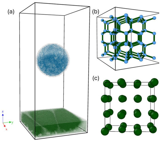
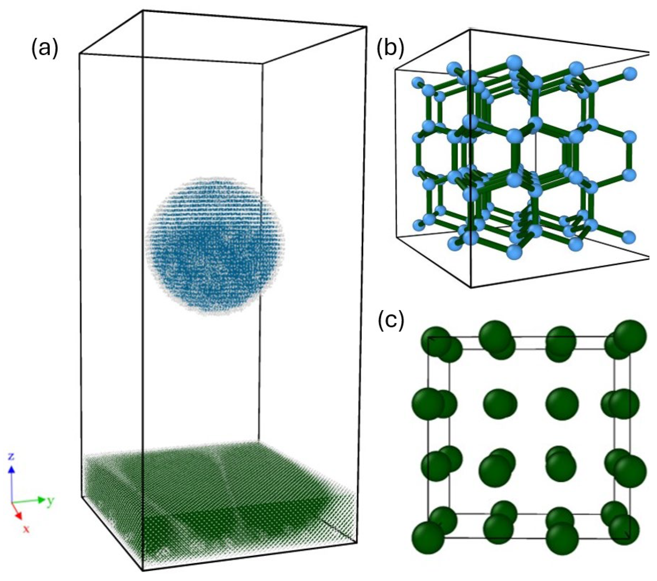
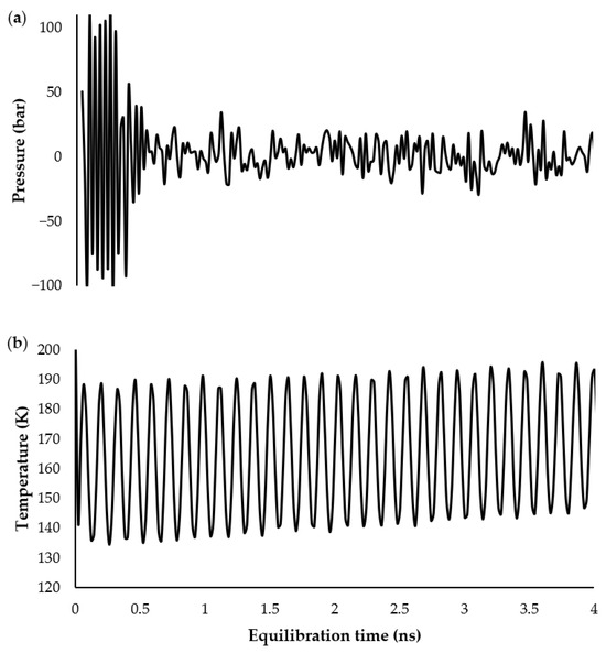
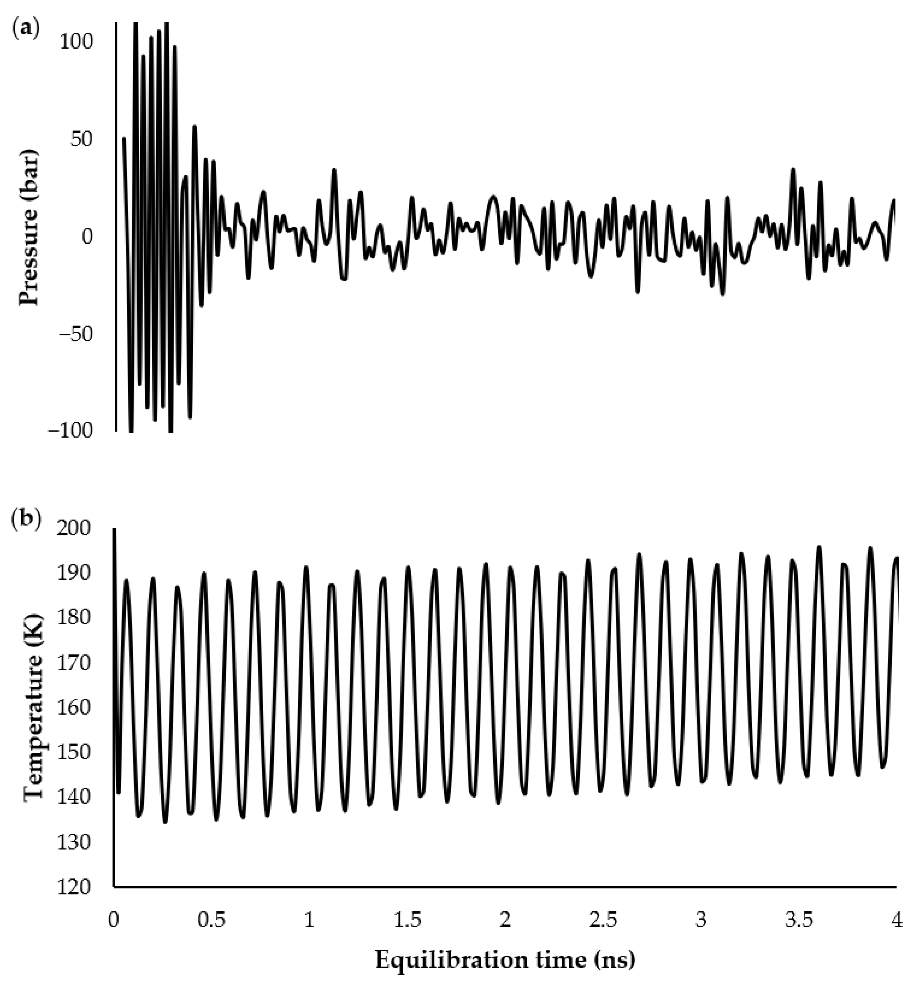
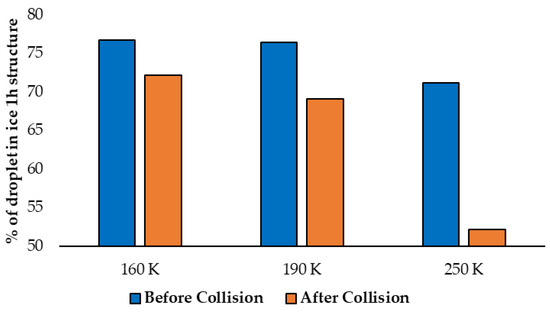
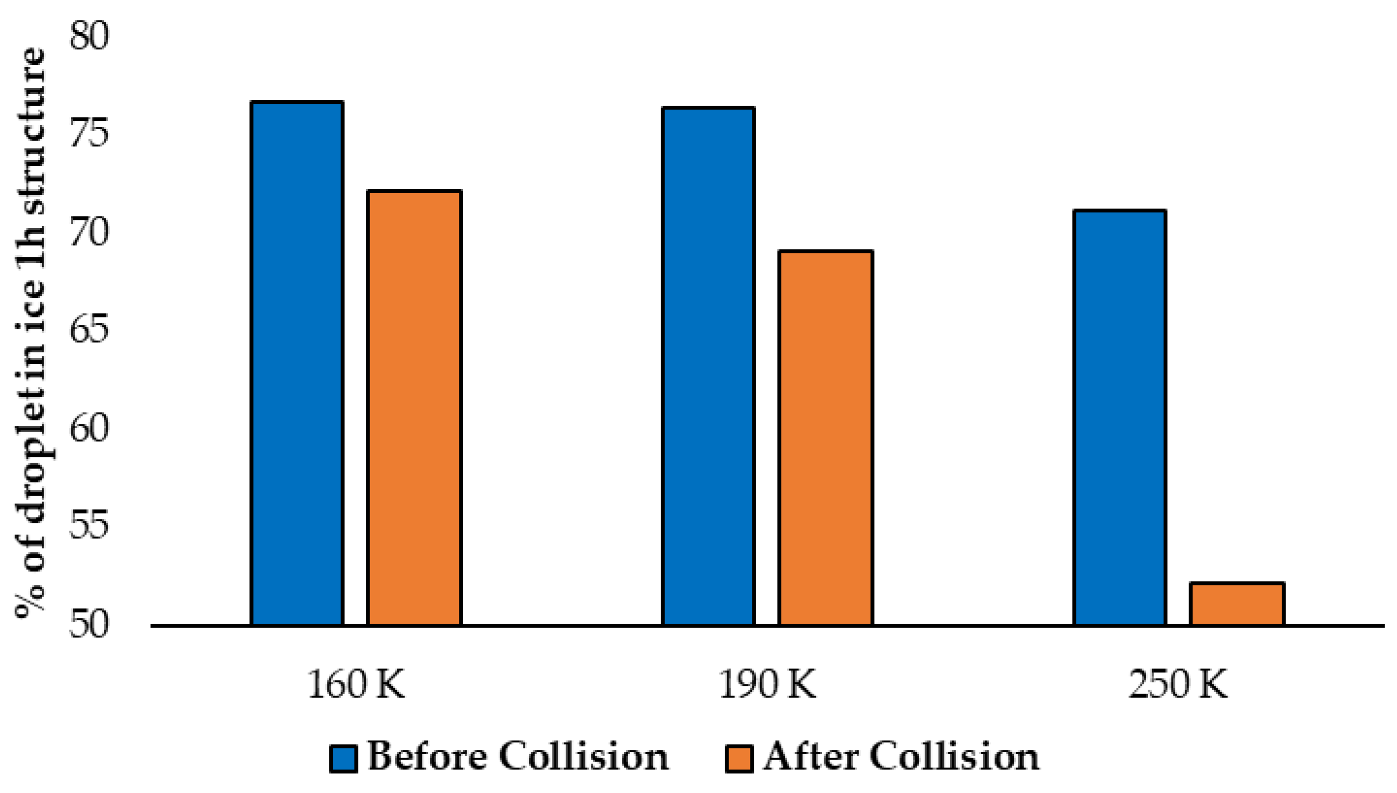
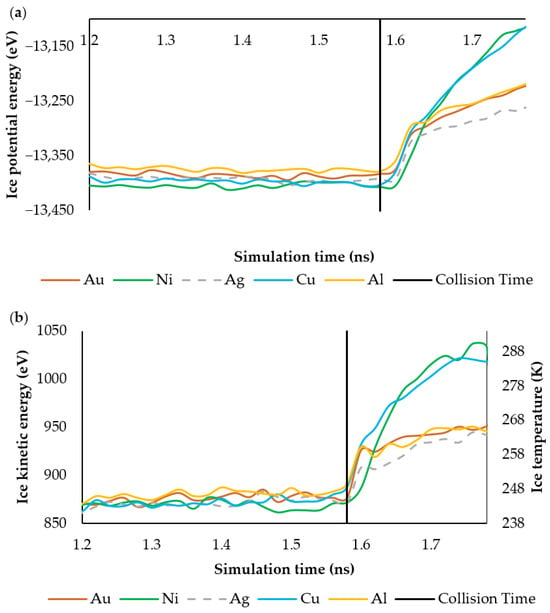
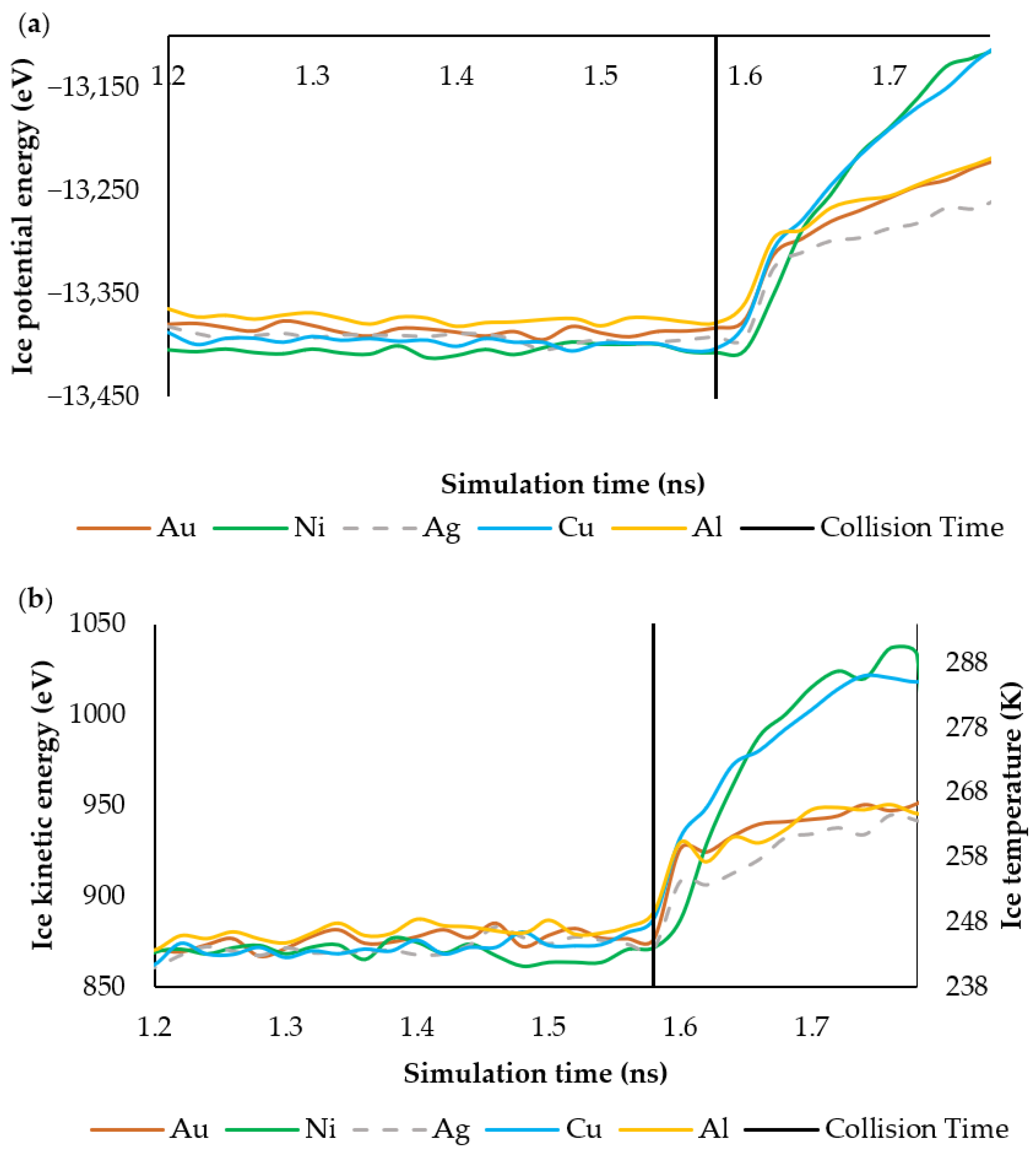
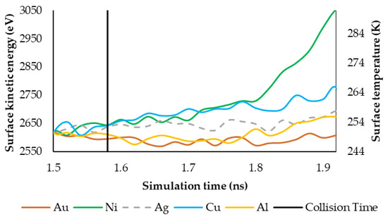
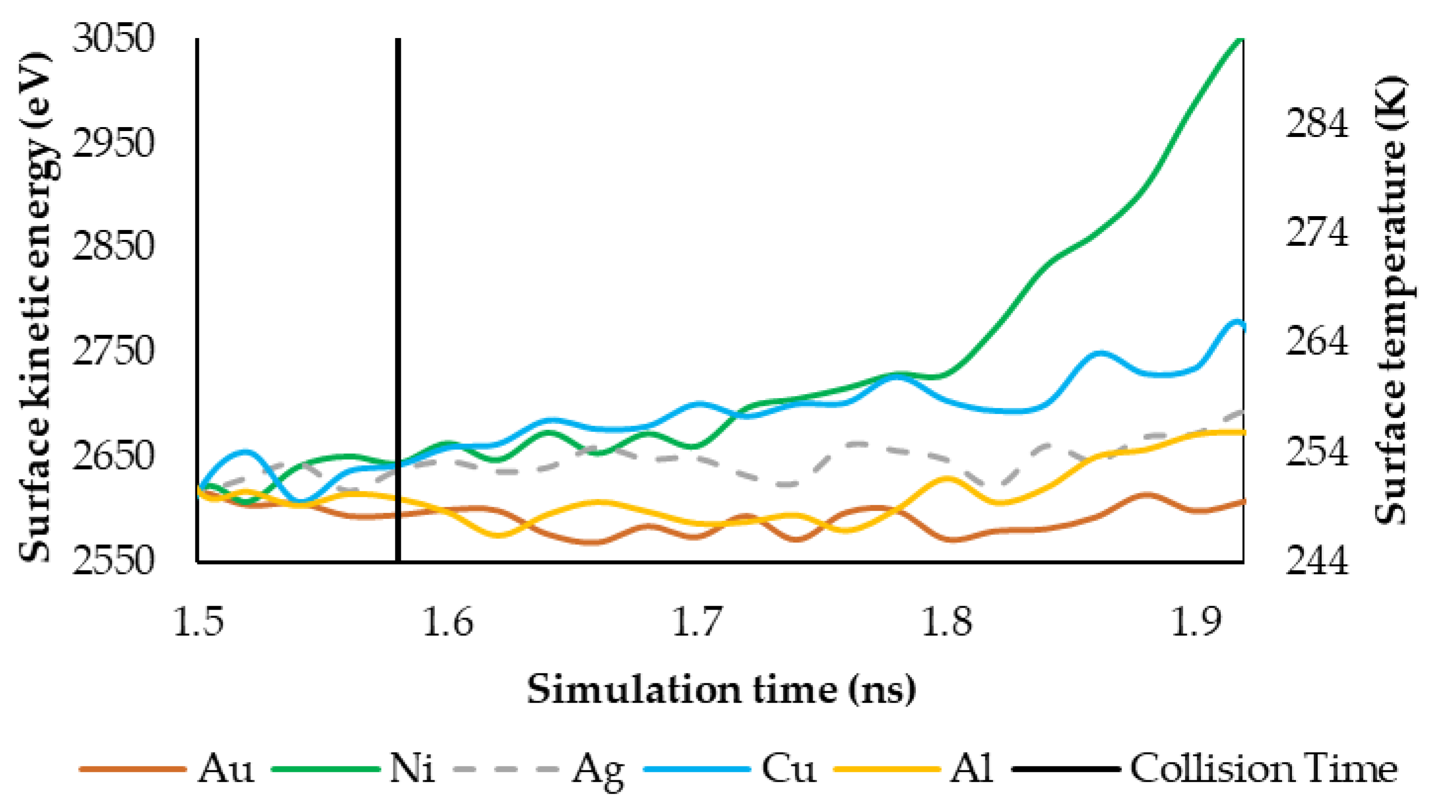
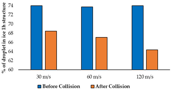
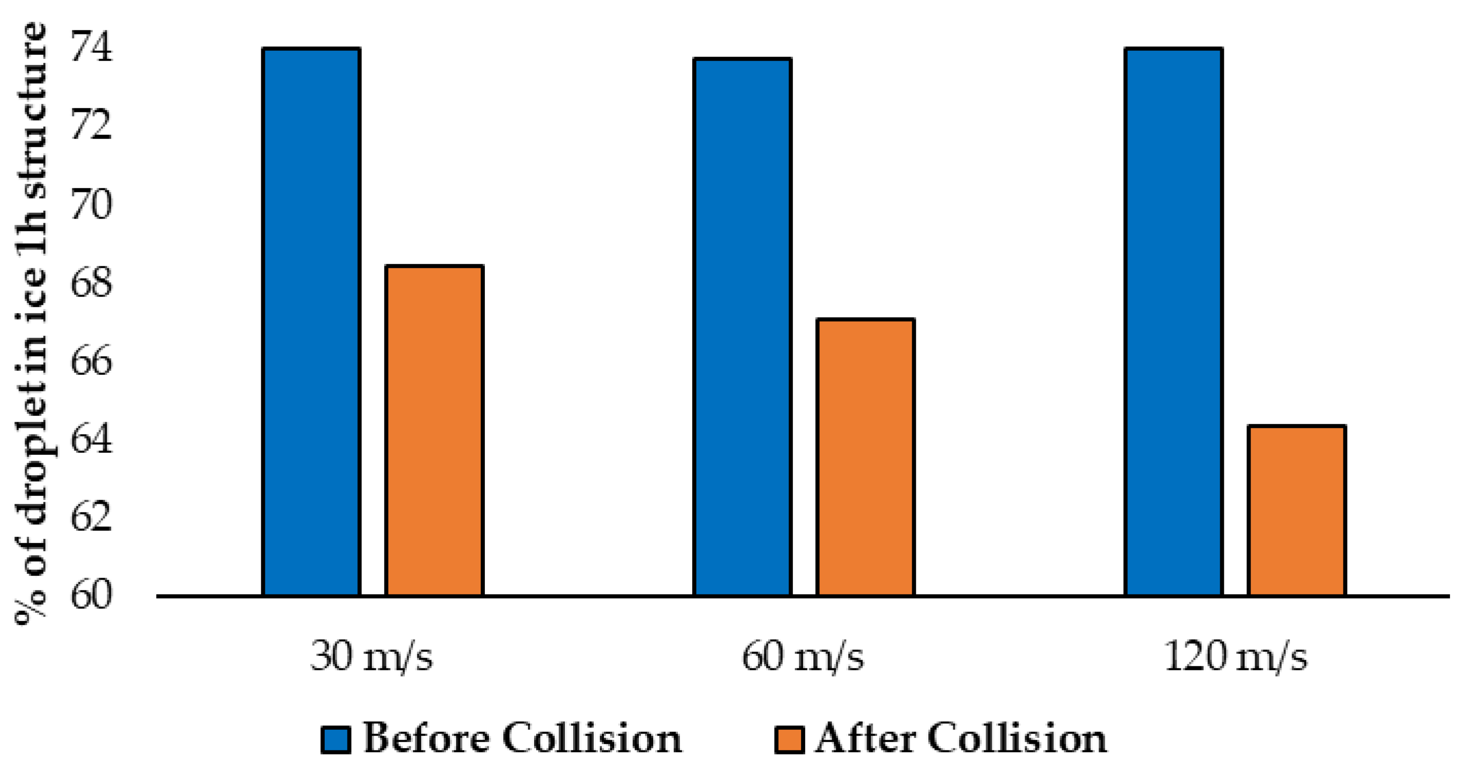
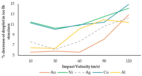
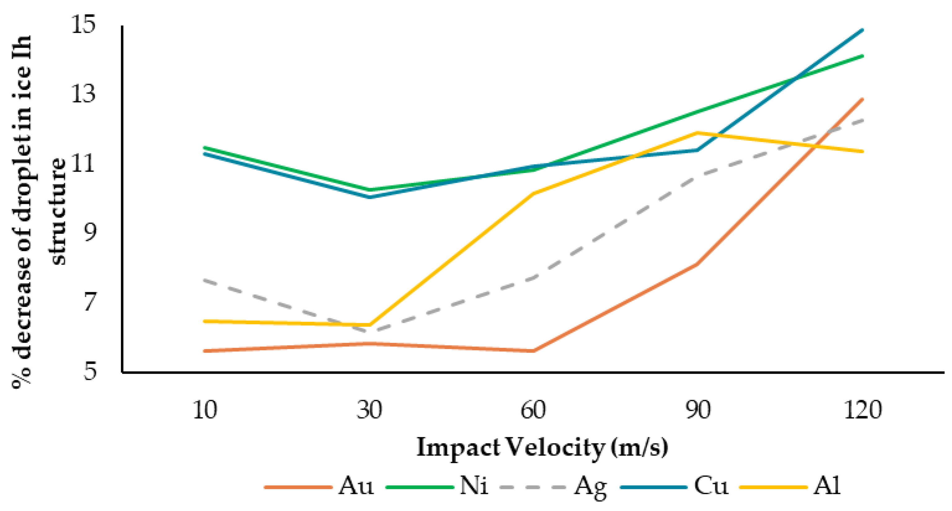
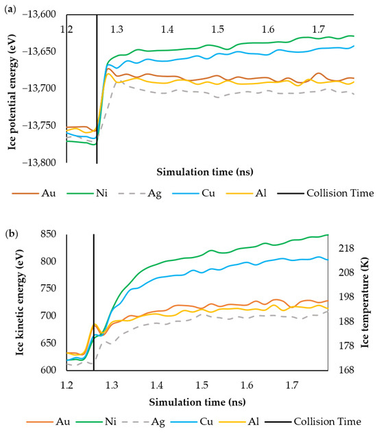
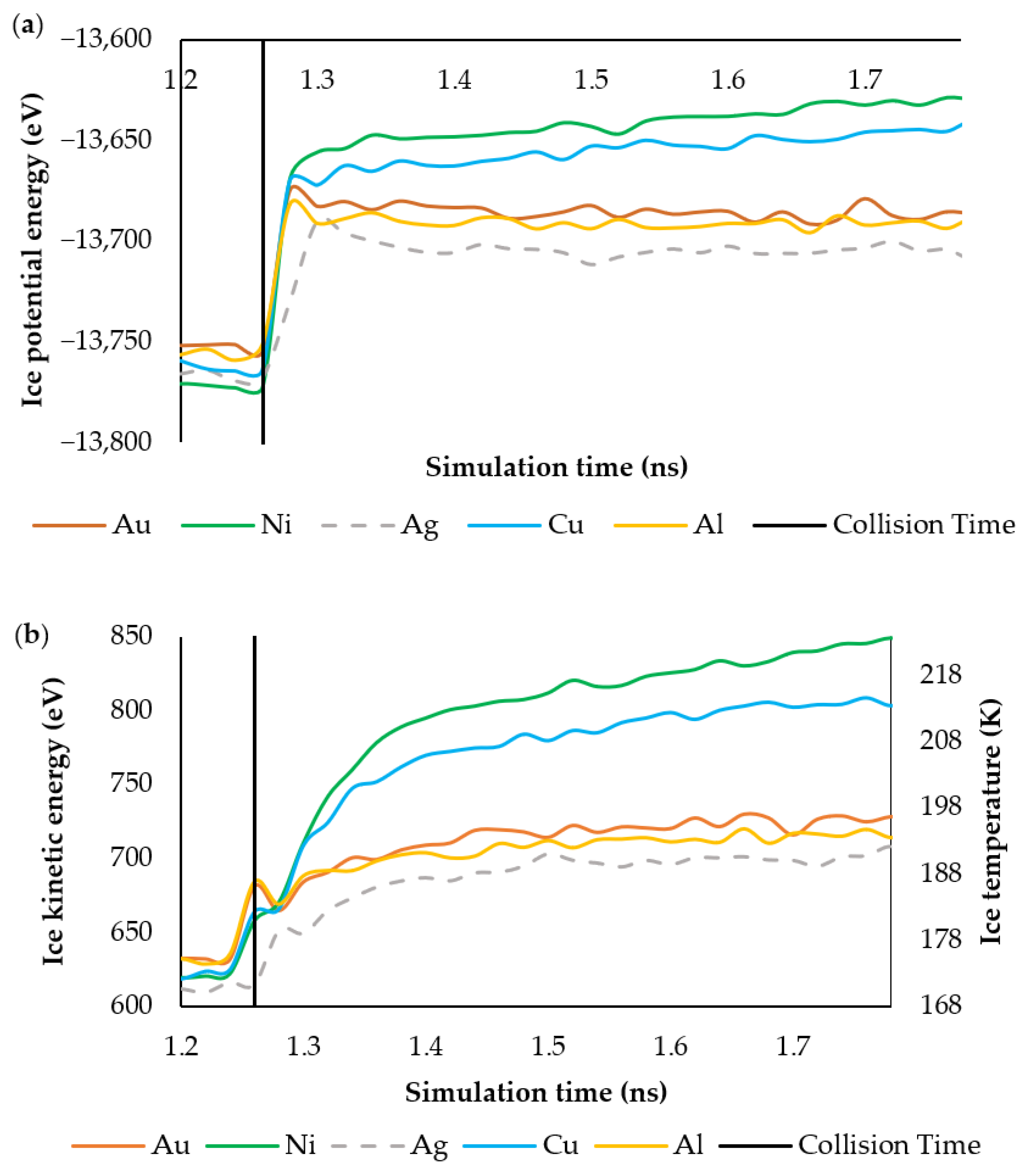
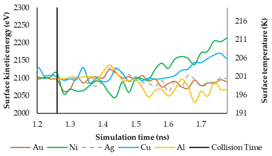
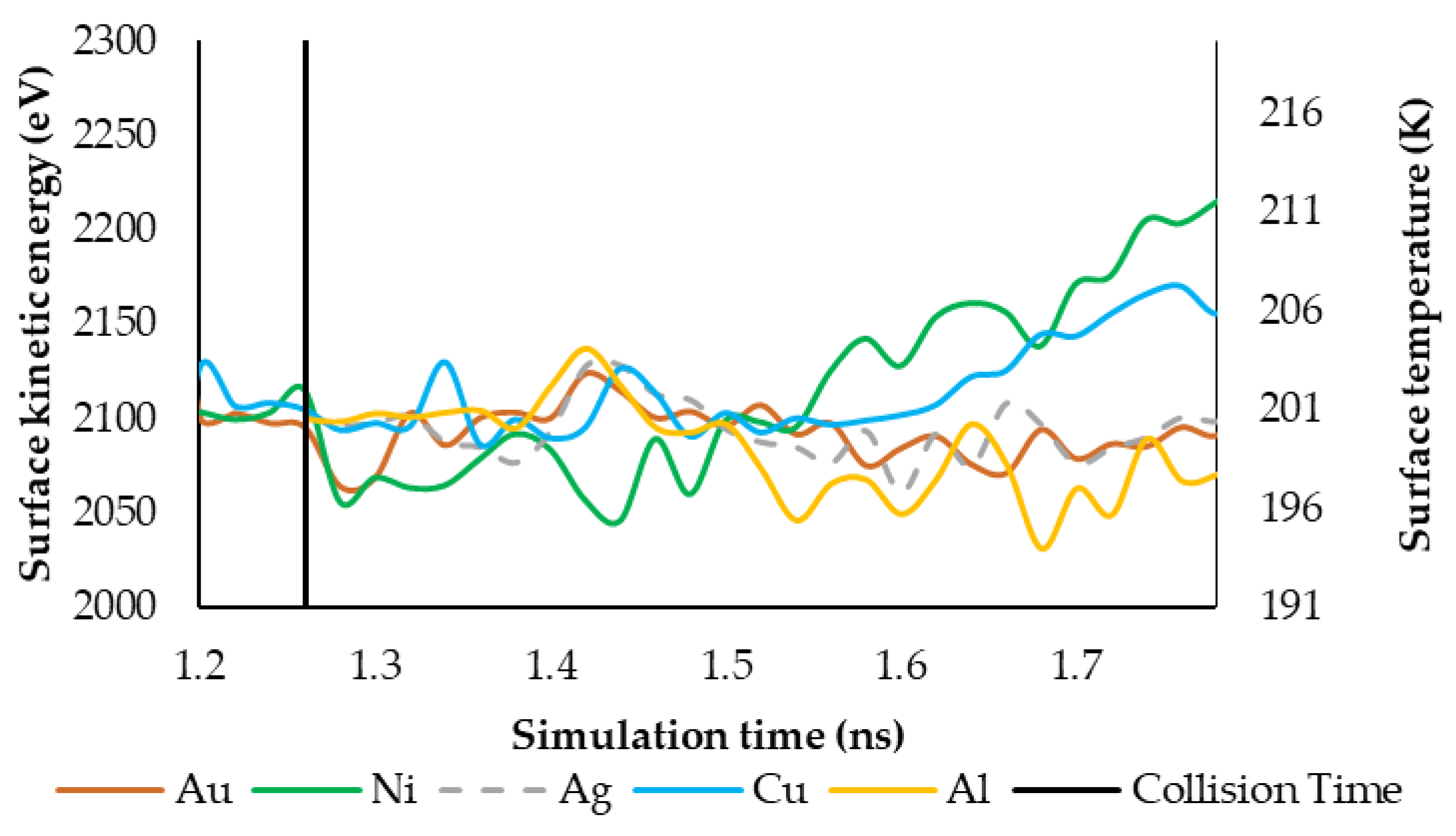
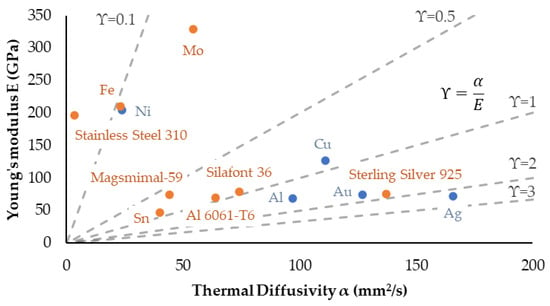
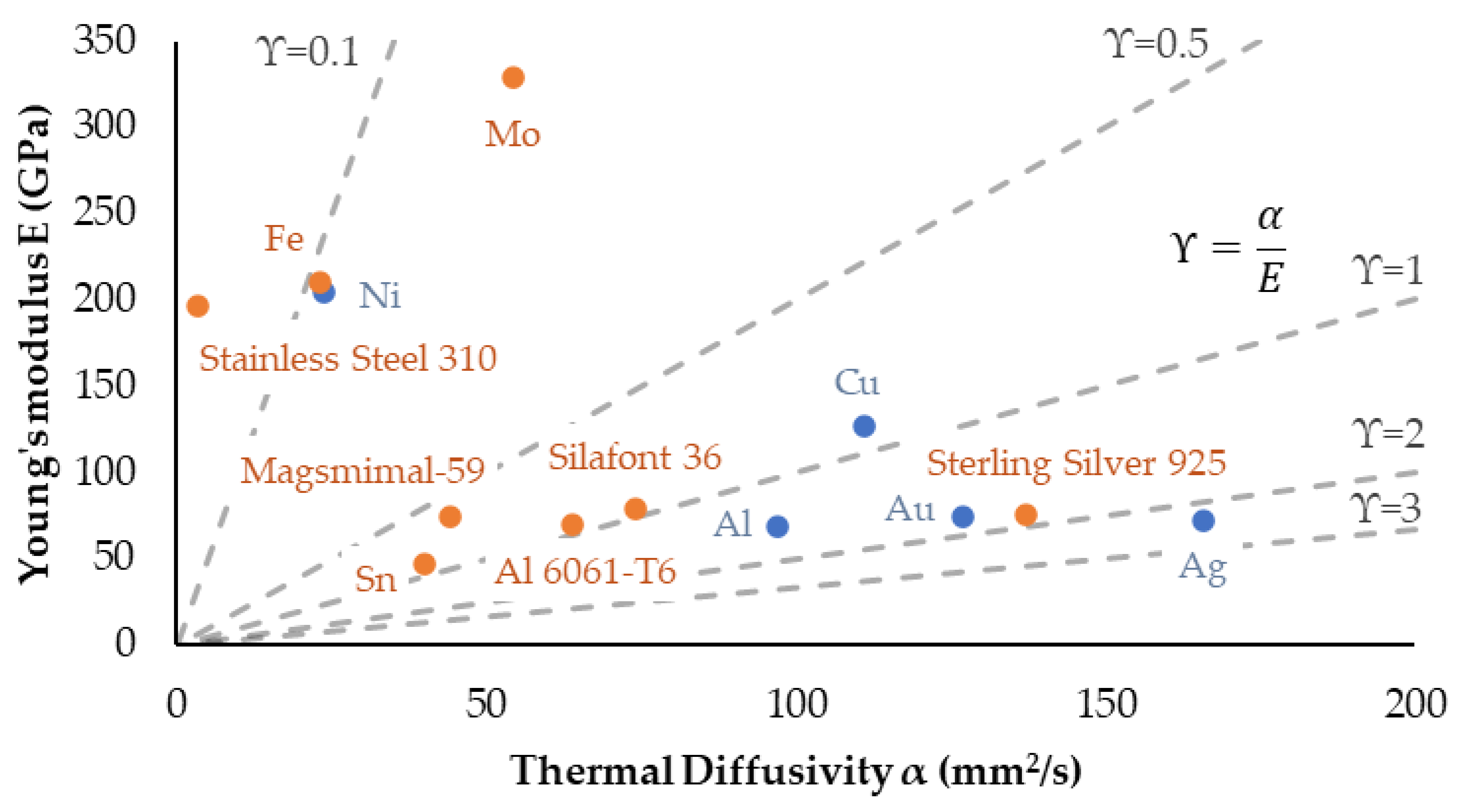
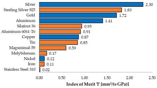
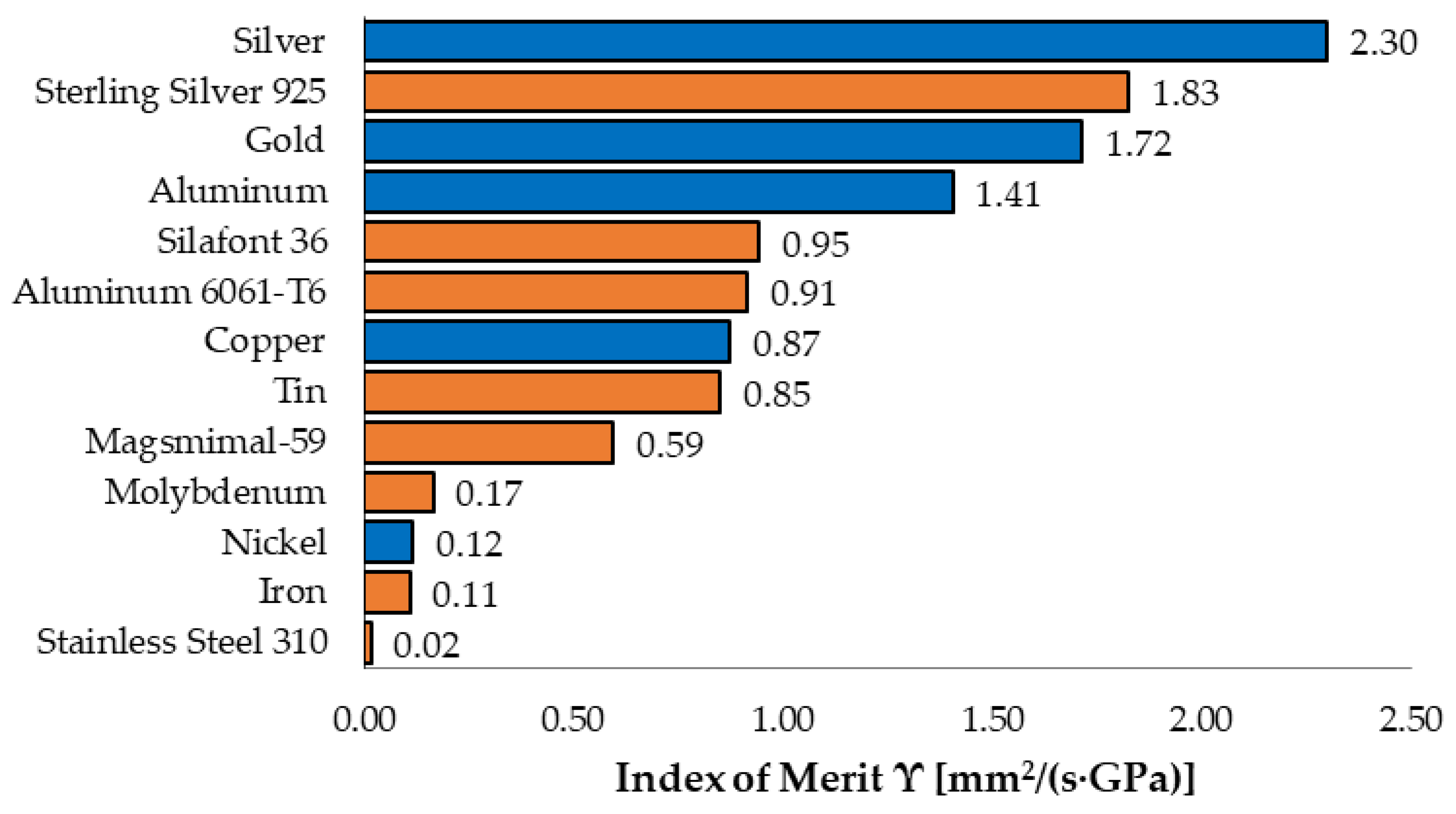
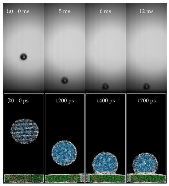
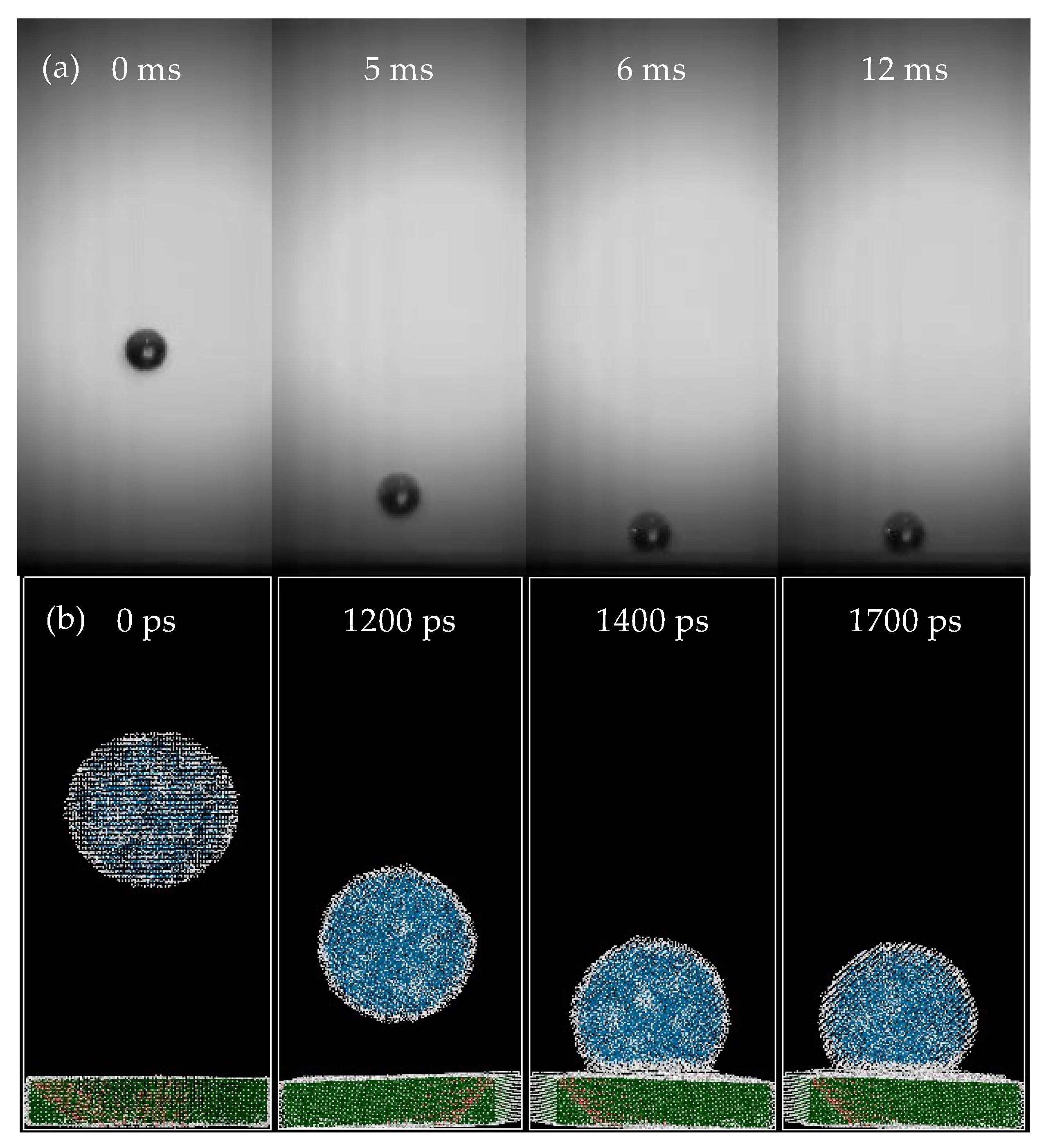
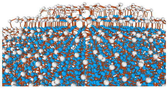
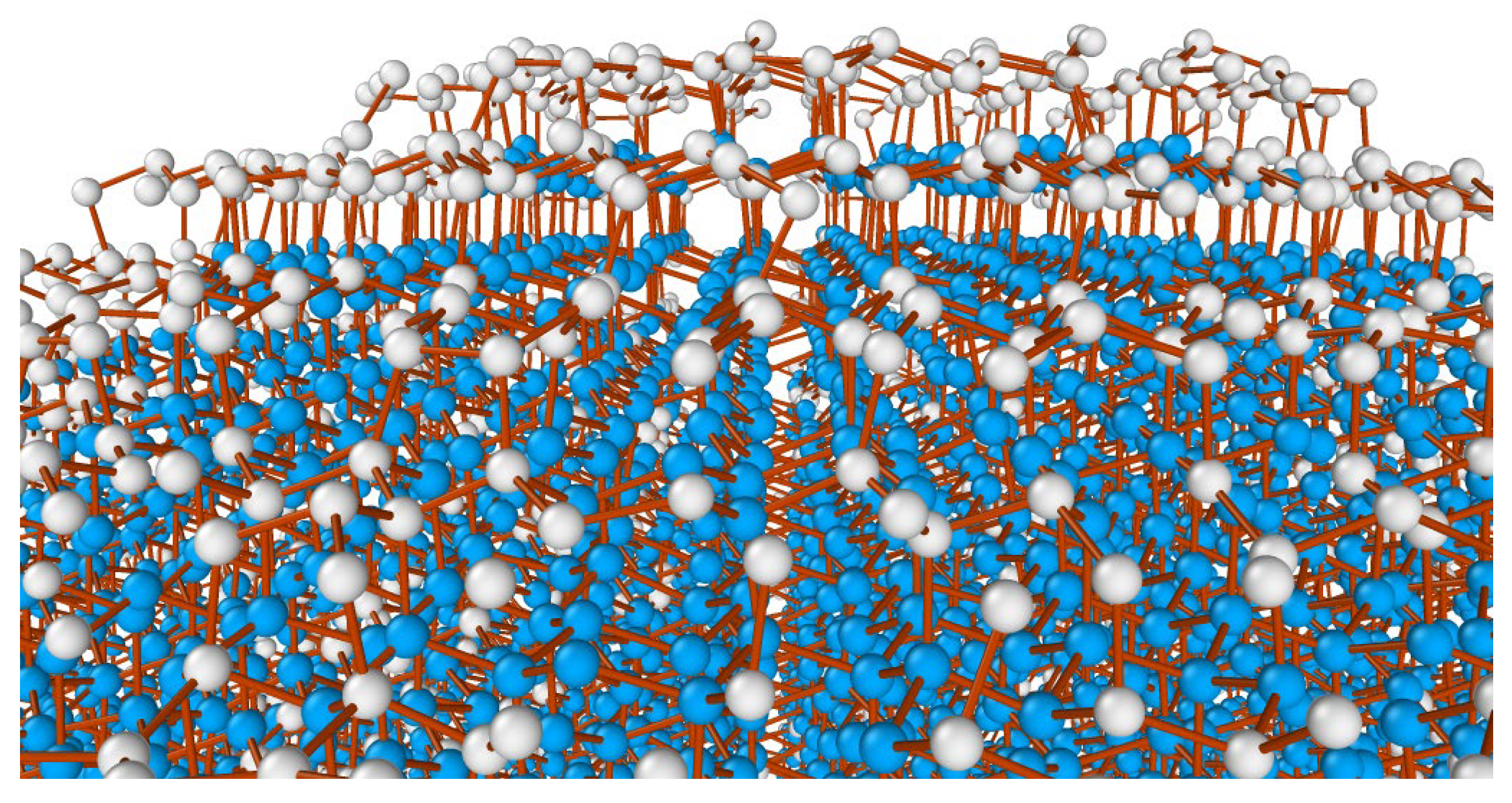
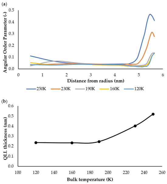
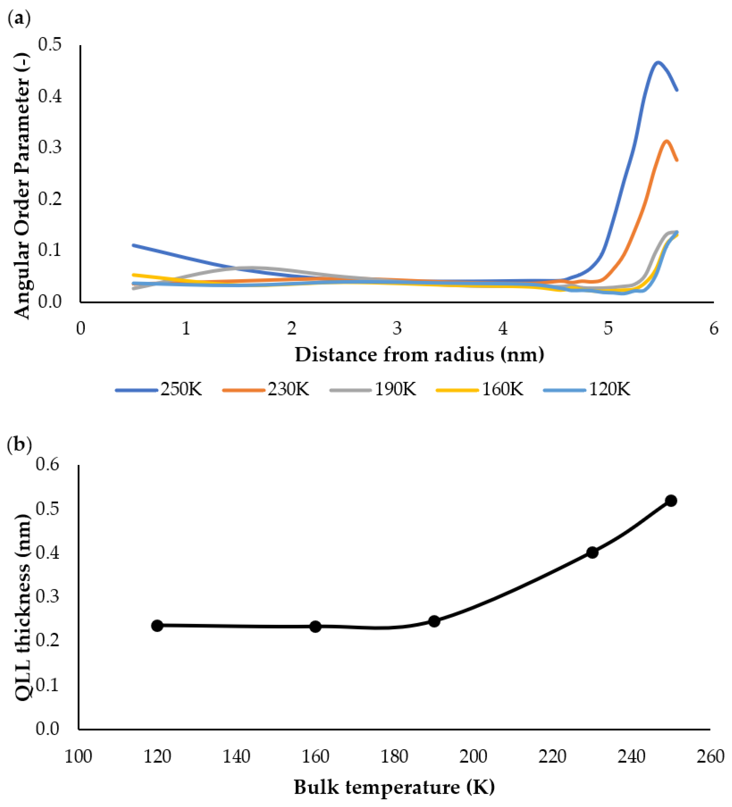

Disclaimer/Publisher’s Note: The statements, opinions and data contained in all publications are solely those of the individual author(s) and contributor(s) and not of MDPI and/or the editor(s). MDPI and/or the editor(s) disclaim responsibility for any injury to people or property resulting from any ideas, methods, instructions or products referred to in the content. |
© 2026 by the authors. Licensee MDPI, Basel, Switzerland. This article is an open access article distributed under the terms and conditions of the Creative Commons Attribution (CC BY) license.