Daytime Sea Fog Detection in the South China Sea Based on Machine Learning and Physical Mechanism Using Fengyun-4B Meteorological Satellite

Highlights

What are the main findings?

• Sea fog spectral sensitivity experiments show that FY-4B spectral characteristics can be transferred to FY-4A.
• Within a machine learning framework with physical constraints, the transfer model improves sea fog detection accuracy.

What is the implication of the main finding?

• With the termination of CALIOP lidar observations in 2023 interrupting access to CALIOP-labeled sea fog samples, we developed a new FY-4B sea fog identification algorithm and an operational FY-4B sea fog product.
• The radiometric transfer approach provides a practical route for migrating algorithms across successor meteorological satellite series.

Abstract

Sea fog is a major meteorological hazard that severely disrupts maritime transportation and economic activities in the South China Sea. As China’s next-generation geostationary meteorological satellite, Fengyun-4B (FY-4B) supplies continuous observations that are well suited for sea fog monitoring, yet a satellite-specific recognition method has been lacking. A key obstacle is the radiometric inconsistency between the Advanced Geostationary Radiation Imager (AGRI) sensors on FY-4A and FY-4B, compounded by the cessation of Cloud–Aerosol Lidar with Orthogonal Polarization (CALIOP) observations, which prevents direct transfer of fog labels. To address these challenges and fill this research gap, we propose a machine learning framework that integrates cross-satellite radiometric recalibration and physical mechanism constraints for robust daytime sea fog detection. First, we innovatively apply a radiation recalibration transfer technique based on the radiative transfer model to normalize FY-4A/B radiances and, together with Cloud-Aerosol Lidar and Infrared Pathfinder Satellite Observation (CALIPSO) cloud/fog classification products and ERA5 reanalysis, construct a highly consistent joint training set of FY-4A/B for the winter-spring seasons since 2019. Secondly, to enhance the model’s physical performance, we incorporate key physical parameters related to the sea fog formation process (such as temperature inversion, near-surface humidity, and wind field characteristics) as physical constraints, and combine them with multispectral channel sensitivity and the brightness temperature (BT) standard deviation that characterizes texture smoothness, resulting in an optimized 13-dimensional feature matrix. Using this, we optimize the sea fog recognition model parameters of decision tree (DT), random forest (RF), and support vector machine (SVM) with grid search and particle swarm optimization (PSO) algorithms. The validation results show that the RF model outperforms others with the highest overall classification accuracy (0.91) and probability of detection (POD, 0.81) that surpasses prior FY-4A-based work for the South China Sea (POD 0.71–0.76). More importantly, this study demonstrates that the proposed FY-4B framework provides reliable technical support for operational, continuous sea fog monitoring over the South China Sea.

1. Introduction

Sea fog is a common hazardous weather phenomenon formed when water vapor in the marine boundary layer condenses into tiny liquid droplets or ice crystals, often resulting in horizontal visibility of less than 1 km [1]. When sea fog occurs, its low visibility significantly disrupts shipping, fisheries, and military operations at sea, underscoring the need for reliable monitoring and early warning. Historically, fog detection relied on sparse observations from coastal stations, ships, and buoys, leaving large areas without coverage.

With the advancement of satellite observation technology, researchers have begun using the radiative differences in passive satellite sensing between fog and clouds for large-scale detection. In 1973, Hunt et al. [2] first used visible and infrared data to analyze the microphysical properties of water and ice clouds, laying the theoretical foundation for subsequent infrared-based cloud studies. John and Bendix [3] analyzed ten years of NOAA-AVHRR data to examine fog frequency and developed a daytime fog detection method using visible and mid-infrared channels, later refined with MODIS multi-band reflectance and radiation transmission models to distinguish low cloud from fog. Wu and Li [4] combined Terra/MODIS data with the two-channel interpolation method (3.7 μm and 11 μm) proposed by Eyer et al. [5], along with auxiliary parameters such as NDSI and NWVI, to develop an automated sea fog detection algorithm for both day and night, achieving an average accuracy of 0.77. Although such thresholding approaches remain widely used, their performance is highly sensitive to solar angle, surface roughness, and atmospheric conditions, leading to instability across seasons and regions.

A major challenge in fog detection based on passive remote sensing lies in distinguishing fog from low cloud, as both exhibit similar optical and microphysical properties. The primary difference is that fog forms in direct contact with the ocean surface, whereas low cloud has an elevated base. Active sensors, such as CALIOP, can resolve cloud-base height with a vertical resolution of 30 m and have been widely used to identify fog and cloud layers. For instance, Badarinath et al. [6] applied CALIOP data to study dense fog over the Ganges Plain, India, demonstrating its viability for fog research. In 2015, Wu et al. [7] combined CALIOP Level-2 VFM products and Level-1 backscatter data for marine fog detection, extracting sample points representing marine fog, low cloud, mid-high clouds, and clear air sea surfaces, which were then applied to MODIS daytime sea fog studies. Given that CALIOP lidar signals attenuate before reaching the fog base, its performance in detecting dense fog is suboptimal. Xiao et al. [8] studied sea fog over the northwestern Pacific, using the MERRA-2 reanalysis dataset to identify true fog from CALIOP candidate layers based on near-surface meteorological variations across different weather conditions (sea fog, stratus, stratus precipitation). The method was validated against ICOADS and five climate stations, yielding an accuracy rate of 0.89 and a false alarm rate of 0.02. Nevertheless, CALIOP’s narrow swath, 16-day revisit cycle, and strong signal attenuation in dense fog limit its capability for continuous monitoring [9]. Passive sensors on geostationary satellites, on the other hand, provide wide-area and high-frequency coverage, but cannot directly observe fog-base height, motivating the use of machine learning to extract nonlinear information from multispectral satellite data.

Recent studies have demonstrated the potential of machine-learning methods to enhance fog detection accuracy. Kim et al. [10] combined GOCI and Himawari-8 data using a Decision Tree (DT) model to identify marine fog over the Yellow Sea, exploiting GOCI’s 412 nm Rayleigh-corrected reflectance and spatial variability indices for fog discrimination, while Himawari-8 infrared data improved cloud removal and edge detection. The method achieved accuracy and hit rates of 0.67 and 0.66, respectively, but its dependence on visible observations limits applicability under certain conditions. Sim and Im [11] later employed Himawari-8 infrared channels as input features for machine-learning models over the Yellow and Bohai Seas, finding that Channel 15 (less affected by water vapor absorption) contributed most to sea-fog detection. Fu et al. [12] integrated Aqua/MODIS and CALIOP data to construct a labeled Arctic sea-fog dataset and compared Random Forest (RF), Support Vector Machine (SVM), multi-layer perceptron (MLP), and fully convolutional network (FCN) algorithms, with the FCN achieving the best balance of detection (0.79) and false-alarm (0.25) rates owing to its ability to capture spatial texture features. To address limited maritime annotations, Xu et al. [13] proposed an unsupervised domain-adaptation framework using terrestrial fog samples and unlabeled oceanic data to generate pixel-level fog masks, achieving high classification accuracy. Despite these advances, most studies still rely primarily on spectral and textural features derived from satellite imagery, often neglecting the physical processes underlying fog formation and development.

To improve the physical validity of sea-fog retrieval, this study integrates previous research on the physical mechanisms underlying sea-fog formation and development [8,14,15,16]. By combining the feature-extraction capability of machine learning with multi-channel observations from the Fengyun-4 (FY-4) geostationary satellite and meteorological reanalysis data, we construct spectral and physically based features that characterize the multidimensional differences between sea fog, other cloud systems, and clear air conditions.

Previous satellite-based fog studies have primarily focused on the Yellow and Bohai Seas [4,7,8,10,11,13,17,18,19,20,21], where fog events occur more frequently, persist longer, and form extensive, continuous layers that are easier for satellites to identify. In contrast, fog over the South China Sea tends to be fragmented, small-scale, and short-lived, strongly influenced by monsoonal circulation, high sea-surface temperatures, and vigorous boundary-layer turbulence [22,23,24]. These factors reduce spatial continuity and detection reliability, making fog recognition over the South China Sea significantly more challenging and thus scientifically valuable.

Furthermore, the termination of CALIOP lidar observations in 2023 and the radiometric discrepancies between FY-4A and its successor, FY-4B, present major obstacles to maintaining operational monitoring continuity. Machine learning models trained on FY-4A data cannot be directly applied to FY-4B because of differences in spectral response functions and calibration coefficients. Therefore, developing a cross-satellite radiometric recalibration and migration strategy is essential to ensure consistency and interoperability between satellite generations.

To address these issues, this study establishes a daytime sea-fog detection machine learning framework for the South China Sea that integrates FY-4A/FY-4B radiometric transfer with physical-mechanism constraints. CALIOP profiles provide single-layer labels (fog, low cloud, mid-high cloud, and clear air), which we spatiotemporally collocate with FY-4 and reanalysis data to construct the spectral/physical input features and Sample dataset. We tune DT, RF, and SVM classifiers using grid search and PSO under stratified 10-fold cross-validation. The resulting models accurately separate fog from clouds and clear air scenes, while FY-4’s continuous wide-area coverage mitigates sparse in situ observations and limited CALIOP overpasses over the open ocean.

2. Materials and Methods

2.1. Study Area

This study focuses on the South China Sea region (18°N–29°N, 107°E–125°E), where research is relatively scarce. This area encompasses the coastal waters of southern China, the Gulf of Tonkin, the Qiongzhou Strait, the Leizhou Peninsula, and the Taiwan Strait (Figure 1). Statistics show that these areas experience an average of 20 or more foggy days annually, predominantly during the winter and spring seasons, with slight variations in the fog season across different regions [22]. These characteristics motivate a winter–spring emphasis in the evaluation and case analyses presented below.

Figure 1. Study area covering the South China Sea (18°N–29°N, 107°E–125°E). The background is a false-color composite generated from FY-4 AGRI bands at 0.65 µm, 0.825 µm, and 12 µm.

2.2. Data Source

2.2.1. FY-4A/FY-4B

FY-4A, China’s second-generation domestically developed geostationary meteorological satellite, was designed and launched in 2016. Its operational data coverage spans from 12 March 2018 to 4 March 2024. The successor satellite, FY-4B, was successfully launched in 2021, with data acquisition commencing on 1 June 2022 and continuing to the present day. In February 2024, FY-4B transitioned from its initial position at 133°E to 105°E, formally replacing FY-4A to assume the primary operational duties. FY-4B carries AGRI, a high-performance instrument capable of acquiring high-frequency, global cloud maps across 15 spectral bands. The satellite offers spatial resolutions ranging from 0.5 to 4 km and provides temporal updates every 15 min. Compared to the AGRI onboard FY-4A, FY-4B incorporates an additional water vapor detection channel and adjusts the spectral characteristics of several channels, enhancing its observational precision, particularly for cloud and fog monitoring.

The FY-4A/4B Level 1 products are provided by the National Satellite Meteorological Centre (NSMC, Beijing, China). Detailed information about the wavelength ranges, center wavelengths, spatial resolutions, and primary applications of each FY-4B channel is provided (Table 1; https://www.nsmc.org.cn/nsmc/cn/satellite/FY4B.html, accessed on 19 May 2025).

Table 1. FY-4B AGRI Band Parameters.

Band	Wavelength Range (µm)	Central Wavelength (µm)	Spatial Resolution (km)	Main Purpose
1	0.45~0.49	0.47	1	Small particle aerosols, true color composition
2	0.55~0.75	0.65	0.5	Vegetation, image navigation, and star observation
3	0.75~0.90	0.825	1	Vegetation, water and atmospheric aerosols
4	1.371~1.386	1.379	2	Cloud recognition
5	1.58~1.64	1.61	2	Low cloud/snow identification, water/ice cloud detection
6	2.10~2.35	2.25	2	Roll clouds, aerosols, large particles
7	3.50~4.00 (High)	3.75	2	High cloud, fire detection
8	3.50~4.00 (Low)	3.75	4	Low reflection target, surface observation
9	5.80~6.70	6.25	4	High cloud target
10	6.75~7.15	6.95	4	Mid-layer water vapor
11	7.24~7.60	7.42	4	Low-layer water vapor
12	8.3~8.8	8.55	4	Cloud, surface temperature
13	10.30~11.30	10.80	4	Surface temperature
14	11.50~12.50	12.00	4	Cloud, total water content, surface temperature
15	13.00~13.60	13.3	4	Water vapor

2.2.2. CALIPSO

The CALIPSO satellite, launched jointly by the National Aeronautics and Space Administration (NASA, Hampton, VA, USA) and Centre National d’Études Spatiales (CNES, Toulouse, France) in 2006, ceased operations in June 2023. It carried a dual-wavelength, polarization-sensitive lidar instrument, CALIOP, operating at wavelengths of 532 nm and 1064 nm. This instrument was capable of observing the vertical structure of clouds and aerosols in the sub-satellite point atmosphere, providing vertical profiling with a resolution of 30 m and horizontal resolution of 333 m below 8 km atmospheric altitude. CALIOP’s Level 1B product offers backscatter data at 532 nm and 1064 nm, as well as sea surface information and MERRA-2 reanalysis data, which includes air temperature, relative humidity, and 10 m level winds. The backscatter data is processed into Vertical Feature Mask (VFM) products, which identify the horizontal and vertical distributions of clouds and aerosols. The VFM product classifies each layer into one of eight categories: null layer, clear atmosphere, cloud layer, tropospheric aerosol, stratospheric aerosol, surface layer, sub-surface layer, and no-signal layer. CALIOP Level 1B and VFM data differ in terms of detection height range, vertical resolution, and horizontal resolution, as detailed in Table 2 and Table 3 (https://www-calipso.larc.nasa.gov/products/, accessed on 19 May 2025). These discrepancies result in variations in the number of latitude-longitude grid points between Level 1B and VFM data. Therefore, to use CALIPSO lidar for sea fog identification, the VFM profile data within the −0.5 to 8.3 km range must be processed to match the latitude-longitude grid of Level 1B, ensuring a vertical resolution of 30 m and horizontal resolution of 333 m.

Table 2. L1B Data Resolution for Different Altitude Ranges.

Altitude Range (km)	Bin Number	Horizontal Resolution (km)	532 nm Vertical Resolution (m)	1064 nm Vertical Resolution (m)	Altitude Zone
30.1~40.0	1–33	5	300	N/A	5
20.2~30.1	34–88	53	180	180	4
8.3~20.2	89–288	1	60	60	3
−0.5~8.3	289–578	1/3	30	60	2
−2.0~−0.5	579–583	1/3	300	300	1

Table 3. VFM Data Resolution for Different Altitude Ranges.

Altitude Region		Vertical Resolution (m)	Horizontal Resolution (m)	Profiles per 5 km	Samples per Profile
Base (km)	Top (km)
20.2	30.1	180	1667	3	55
8.2	20.2	60	1000	5	200
−0.5	8.2	30	333	15	290
Total					545

2.2.3. ERA5

ERA5 is the fifth-generation reanalysis of global climate and weather data over the past 80 years, produced by the European Centre for Medium-Range Weather Forecasts (ECMWF, Reading, UK), with data available from 1940 onwards (https://cds.climate.copernicus.eu/datasets/reanalysis-era5-single-levels, accessed on 19 May 2025). The ERA5 data utilized in this study include sea surface temperature (SST). The spatial resolution of the data is 0.25° × 0.25°.

2.3. Methods

2.3.1. Extraction of Sea Fog Labels

This study leverages CALIOP’s high vertical resolution below 8 km to extract four sample categories: sea fog, clear air, low cloud, and mid-high cloud. This requires the combined use of CALIOP Level-1B and VFM Level-2 products: Level-1B provides essential data, including longitude, latitude, scan profile time, 532 nm backscatter total attenuation coefficient, altitude, and land/sea surface information, enabling precise positioning and surface type identification. The VFM product provides layer-type identifiers with a 30 m vertical resolution at corresponding spatio-temporal coordinates.

According to the World Meteorological Organization (WMO) cloud definitions (https://cloudatlas.wmo.int/en/clouds-definitions.html, accessed on 19 May 2025), mid-high clouds are defined as those with altitudes above 2 km, while low clouds are those below 2 km. For the study region, primarily coastal sea fog in South China, simulations of relative humidity variations suggest sea fog heights of approximately 300–400 m [23], with mature-stage sea fog tops estimated around 100 m [24]. Based on this, in this study, under conditions where the CALIOP land–sea information (Ocean Mask) indicates an oceanic surface, cloud features (Cloud, VFM classification 2) detected at altitudes above 2 km are labeled as mid-high cloud, while cloud features between 500 m and 2 km are labeled as low cloud. Samples not classified as sea fog, low cloud, or mid-high cloud are designated as clear air.

The algorithm for extracting sea fog sample labels follows the method proposed by Wu et al. [7], treating sea fog as a cloud in direct contact with the sea surface, as it occurs within the atmospheric boundary layer. Therefore, cloud feature labels at altitudes between 10 and 40 m above the mean sea level are identified as sea fog. Wu et al. [25] also addressed the issue of CALIOP potentially confusing sea fog with the underlying sea surface during observation, known as the sea surface misclassification problem. They suggest that when a VFM product’s track point is located at an altitude greater than 40 m and the 532 nm backscatter coefficient in Level 1B data exceeds 0.03 km⁻¹·sr⁻¹, the surface feature layer (Surface, VFM classification 5) should be classified as sea fog, not as the sea surface. Furthermore, due to CALIOP’s signal attenuation when penetrating clouds, leading to the identification of no signal for the sea surface, this study also classifies feature data at altitudes of 10–40 m as no signal and 40–70 m as cloud, both as sea fog. The detailed process for extracting sea fog labels is illustrated (Figure 2), which shows the CALIOP sea fog detection algorithm flowchart.

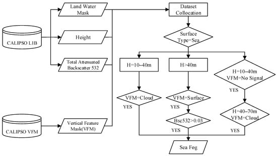
Figure 2. Sea Fog Detection Algorithm Based on CALIOP.

Due to the limitations of the AGRI instrument on the FY-4 satellite, which captures radiation from the entire atmospheric column without distinguishing between different altitudes, this study uses only single-layer clouds, single-layer fog, and unobstructed clear air extracted from CALIOP data as samples. These samples are spatially and temporally matched, ensuring that all CALIOP samples within each 4 km × 4 km grid pixel of the FY-4 are classified as the same type, ultimately forming a sample set with a 4 km horizontal resolution. Figure 3 presents a false-color FY-4A image alongside the corresponding CALIOP VFM image, illustrating the spatial correspondence between the two datasets.

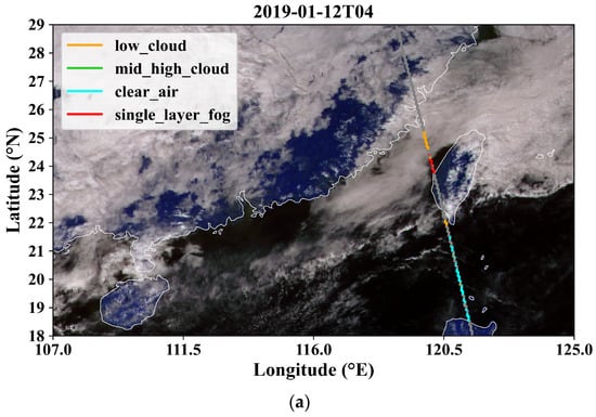
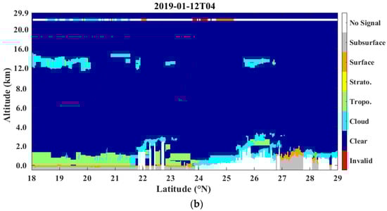
Figure 3. (a) shows the FY-4A false-color image, while (b) shows the CALIOP VFM image (World real-time: 12 January 2019, 04:53:40 UTC). Panel (a) is a false-color image synthesized from the 0.47 µm, 0.65 µm, and 0.825 µm visible channels of FY-4A, with the straight line representing the CALIOP track. Panel (b) displays the CALIOP VFM image, where the color scale on the right indicates the eight feature categories of the VFM product, listed from top to bottom as: no signal, subsurface, surface, stratospheric aerosol, tropospheric aerosol, cloud, clear air, and invalid. The color-coded horizontal strip at the top of the VFM image (b) represents the classification results along the CALIOP track, which is directly projected from panel (a). The color scheme is consistent across both panels: red indicates sea fog, blue denotes clear air, orange signifies low cloud, and green represents mid-high cloud (note: mid-high cloud samples were not present during this specific time step).

2.3.2. Transfer Model

To ensure the continued validity of sea fog classification models that were developed using CALIOP data (which ceased operations in June 2023), this study employed a transfer model for both FY-4A AGRI and FY-4B AGRI proposed by Yu et al. [26]. This approach enabled interoperability and consistency in the radiometric characteristics between the two satellites, ensuring seamless integration of their data into the model training dataset.

The transfer model between FY-4A/4B AGRI satellites is based on two core technologies: cross-calibration and radiative transfer simulation. The model utilizes high-precision reference sensors or radiative simulation results to establish transferable relationships between the radiative response functions or calibration parameters of sensors mounted on different satellites, ensuring interoperability and consistency in radiometric characteristics. The technical workflow involves: (1) integrating multi-source atmospheric data (e.g., ERA5) to obtain temperature-humidity profiles, surface temperature, albedo, emissivity, and observational geometry parameters, combined with different climate types, aerosol models, cloud cover conditions, and surface types to create a multi-scenario dataset; (2) performing high-precision radiative transfer simulations using MODTRAN 6.0+ (Spectral Sciences, Inc., Burlington, MA, USA) to generate hyperspectral radiance data with 0.2 cm⁻¹ resolution; (3) conducting channel-level spectral convolution through weighted integration to derive radiant brightness temperatures (infrared bands) or apparent reflectance (visible/near-infrared bands); (4) constructing radiometric conversion models via least squares or partial least squares (PLS) regression, using linear/quadratic polynomial functions or segmented look-up tables (LUTs); and (5) applying bidirectional calibration to correct radiometric consistency between historical FY-4A and FY-4B data. This study converted FY-4B AGRI channels to align with FY-4A’s 14 AGRI channels, ensuring temporal continuity and resolving the continuity issue in sea fog detection.

2.3.3. Constructing the Input Features and Sample Dataset

Given that sea fog in the South China Sea mainly occurs in winter and spring, we restrict the analysis to these months (December through April) from 2019 to 2023. A total of 107 CALIOP tracks that detected fog over the South China Sea were selected, resulting in 755 single-layer sea fog samples. For the years 2019–2022, labels were extracted using FY-4A data. In 2023, FY-4B data were used, which were radiometrically transferred to ensure consistency with FY-4A via the FY-4A/B AGRI transfer model. The temporal distribution of labeled samples by year and by season is summarized in Table 4.

Table 4. Temporal distribution of labeled samples. Counts are summarized by year and by season for all available labeled samples prior to any downsampling. Seasons are defined as Winter (December–February) and Spring (March–April).

Group	Low Cloud	Mid-High Cloud	Clear Air	Sea Fog	Total	% of All Samples
By year
2019	620	172	689	128	1609	18.8%
2020	277	177	531	56	1041	12.1%
2021	679	439	672	244	2034	23.7%
2022	457	569	1013	182	2221	25.9%
2023	378	454	688	145	1665	19.4%
By season
Winter (December–February)	1628	1090	1846	458	5022	58.6%
Spring (March–April)	783	721	1747	297	3548	41.4%
Total (2019–2023)	2411	1811	3593	755	8570	100%

A comprehensive candidate set of 21 features was constructed based on the characteristic differences between low cloud, mid-high cloud, sea fog, and clear air. These features, summarized in Table 5, cover spectral, textural, and physical mechanisms and serve as the baseline input for subsequent model training and feature optimization. Reflectance features were derived from channels at 0.47, 0.65, 0.825, 1.61, and 2.25 μm, while BT features were derived from the 3.75, 10.7, and 12 μm channels at 4 km × 4 km resolution. Two auxiliary parameters were additionally included to improve sea-fog discrimination, including BT10.7–SST, where SST from ERA5 (0.25° × 0.25°) was bilinearly resampled to the FY-4 grid. Physical-mechanism parameters were derived from the CALIOP Version 4 L1B auxiliary meteorological fields, including 10 m wind components (surface_wind_speeds_10m_u and surface_wind_speeds_10m_v), temperature inversion strength (T1000m−T50m, where T denotes temperature), and relative humidity at 50 m, 1000 m, and 2000 m. The selection of these variables and vertical levels was constrained by the CALIOP L1B product and its Met_Data_Altitudes structure: for the shallow fog layer targeted in this study (<2 km), only three nodes (0.05, 1.04, and 2.05 km) are available; therefore, these levels were adopted to represent the near-surface layer, the upper marine boundary layer, and the lower free troposphere, respectively. Detailed feature analysis is presented in Section 3.1 and Section 3.2.

Table 5. List of the initial 21-dimensional candidate feature set constructed for sea fog detection.

	Sample Feature	Meaning	Application
Spectral Features *	Ref 0.47, Ref 0.65, Ref 0.825	Visible and near-infrared reflectance	clear air vs. cloudy/fog
	Ref 1.61, Ref 2.25	Shortwave infrared reflectance	ice/snow and clouds
	BT3.75H, BT3.75L, BT10.7	Mid- and longwave infrared brightness temperature	clear air vs. cloudy/fog
	DBT10.7–12, DBT8.5–10.7, DBT3.75L–10.7	Mid- and longwave infrared brightness temperature difference	Particle scale
	BT10.7–SST	Atmospheric window brightness temperature and SST difference	Cloud/fog top height
	STDbt10.7	Standard deviation of long-wave infrared in a 2 × 2 window	Texture feature
	NDSI 0.47–2.25	Normalized Difference Snow Index	ice/snow and clouds
Physical-mechanism Features	Surface_wind_speeds_10m_u, Surface_wind_speeds_10m_v	Ground-level wind	Wind direction and speed
	T1000m−T50m	Temperature inversion	Atmospheric stability
	RH_50m, RH_1000m, RH_2000m	Relative humidity	Water vapor content
	Year	Time	Inter-annual variations

* The numbers in the “Spectral Feature” rows represent the wavelength, where Ref stands for reflectance, BT stands for brightness temperature, and DBT stands for brightness temperature difference.

2.3.4. Model Configuration and Optimization

This study employed three machine learning algorithms, DT [27], RF [28], and SVM [29], for daytime sea-fog detection. To address the class imbalance [30] and prevent sea fog samples from being underrepresented (sea fog accounts for only 8.8% of all samples), the other categories (clear air, low cloud, and mid–high cloud) were randomly downsampled to match the sea-fog class (755 samples). This process yielded a class-balanced modeling dataset totaling 3020 samples. The balanced dataset was then divided into a stratified 80/20 split for training and independent testing. Within the training subset, hyperparameters were tuned using stratified 10-fold cross-validation (StratifiedKFold) [31], and the held-out test set was used only for final performance reporting.

The DT model used the CART algorithm with the Gini impurity index to determine feature splits. The key parameters include the maximum tree depth (max_depth), which controls the degree of tree expansion and model complexity, minimum samples per split (min_samples_split), and minimum samples per leaf (min_samples_leaf), which determines the smallest number of samples required to create a new branch. Both parameters were tuned to avoid overfitting and improve generalization.

The RF model consisted of multiple CART trees built on bootstrap resampling and majority voting. The main parameters were the number of trees (n_estimators) and maximum tree depth (max_depth). These were adjusted to balance bias and variance and to ensure robust ensemble performance.

The SVM used a Gaussian (RBF) kernel to capture nonlinear separability among clear air, fog, and cloud samples. The penalty coefficient (C) controls the trade-off between margin width and classification error, while the kernel parameter (γ, gamma) determines the influence range of each training sample in the feature space.

To minimize manual bias in parameter selection, three optimization strategies were applied: 10-fold cross-validation, grid search [32], and PSO [33]. In 10-fold cross-validation, the training set was divided into 10 subsets, each serving once as the validation set while the remaining nine were used for training [34]. StratifiedKFold ensured that all four classes (clear air, sea fog, low cloud, and mid-high cloud) were represented in each subset, reducing class-imbalance bias. Grid search was applied to tune discrete parameters in DT and RF. PSO was used to optimize continuous hyperparameters in SVM, where particles iteratively updated their positions based on individual and global best solutions until convergence to the optimal configuration.

2.3.5. Evaluation Metrics

Feature inputs from the test set were fed into the trained machine learning models to generate classification results. By comparing the dataset’s truth labels with the predicted outcomes, a confusion matrix was used to evaluate classification performance (Table 6).

Table 6. Confusion Matrix.

	CALIOP Detection Positive	CALIOP Detection Negative
Model Detection Positive	True Positive (TP)	False Positive (FP)
Model Detection Negative	False Negative (FN)	True Negative (TN)

Model performance is evaluated using confusion matrices to calculate precision, recall (also referred to as the Probability of Detection, POD), F1-score, accuracy, Critical Success Index (CSI), and Macro-average F1-score, following the systematic analysis of performance measures by Sokolova and Lapalme [35].

Precision measures the proportion of correctly predicted positive samples among all predicted positives, while Recall measures the model’s ability to correctly identify true positive samples. The F1-score, which represents the harmonic mean of precision and recall, is particularly suitable for imbalanced classification tasks. Accuracy reflects the overall correctness of classification results. The CSI evaluates the fraction of observed or forecast events that were correctly predicted, effectively penalizing both false alarms and misses. Finally, the Macro-F1 provides a global assessment of multiclass performance by calculating the unweighted mean of F1-score across all N categories (here N = 4), treating all classes as equally important regardless of sample size.

The formulas for these metrics are as follows:

$$\mathrm{Precision}={\displaystyle \frac{\mathrm{TP}}{\mathrm{TP}+\mathrm{FP}}}$$

(1)

$$\mathrm{Recall}={\displaystyle \frac{\mathrm{TP}}{\mathrm{FN}+\mathrm{TP}}}$$

(2)

$$\mathrm{F}1-\mathrm{score}=2\times {\displaystyle \frac{\mathrm{Precision}\times \mathrm{Recall}}{\mathrm{Precision}+\mathrm{Recall}}}$$

(3)

$$\mathrm{Accuracy}={\displaystyle \frac{\mathrm{TP}+\mathrm{TN}}{\mathrm{TP}+\mathrm{TN}+\mathrm{FP}+\mathrm{FN}}}.$$

(4)

$$\mathrm{CSI}={\displaystyle \frac{\mathrm{TP}}{\mathrm{TP}+\mathrm{FP}+\mathrm{FN}}}$$

(5)

$$\mathrm{Macro}-\mathrm{F}1={\displaystyle \frac{1}{N}}{{\displaystyle \sum }}_{i=1}^N{\mathrm{F}1-\mathrm{score}}_i$$

(6)

3. Results

3.1. Analysis of Candidate Spectral Characteristics

3.1.1. Reflectance

The spectral characteristics of different atmospheric targets were analyzed using clear air, low cloud, single-layer fog, and mid–high cloud samples. Figure 4 and Figure 5 present the top of atmosphere reflectance characteristics across multiple spectral bands. Figure 4 specifically illustrates the interannual variation in mean reflectance values for samples collected in 2019, 2022, and 2023. This variation may result from interannual spectral differences in sea fog and other atmospheric targets or from minor instrumental biases, leading to distinct distributions of mean reflectance and reflectance variability among different samples. Panel (c) in Figure 4 shows FY-4B AGRI reflectance that has been migrated into the FY-4A radiometric domain using the cross-satellite transfer model (see Section 2.3.2). Because FY-4A and FY-4B occupy different sub-satellite longitudes, they observe the same target along different optical paths, making a direct channel-to-channel comparison between them infeasible.

Figure 4. Spectral sensitivity analysis showing the variation in mean reflectance across different wavelengths (0.47, 0.65, 0.825, 1.375, 1.61, and 2.25 µm) for the four sample categories. The markers and connecting dashed lines represent the mean reflectance values and the overall spectral response trends for each target type across the bands. The error bars represent the 95% confidence interval (95% CI), estimated via bootstrapping, which indicates the uncertainty associated with the mean reflectance for each category.

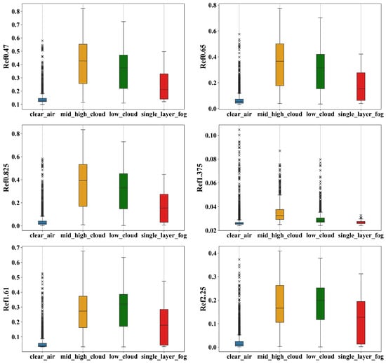
Figure 5. Distribution of reflectance for the four sample categories across different spectral bands (using 2019 as an example). The central horizontal line in each box represents the median, while the top and bottom edges of the box indicate the 75th and 25th percentiles (interquartile range, IQR), respectively. The whiskers (error bars) extend to 1.5 times the IQR from the box edges, covering the range of data points excluding outliers. Individual outliers are marked with “x”.

Overall, in the 1.375 μm near-infrared band, the differences among the samples are minimal, with mean variations below 0.03 across three years of data. Therefore, the reflectance channel at 1.375 μm is excluded from the feature matrix for the sample dataset. Clear air samples show significant reflectance differences compared to other samples, except in the 1.375 μm channel. Figure 5 further reveals that single-layer sea fog and mid/low cloud samples exhibit overlapping reflectance spectral characteristics in the visible band (e.g., 0.47 μm, 0.65 μm), near-infrared band (0.825 μm), and shortwave infrared bands (e.g., 1.61 μm, 2.25 μm). This overlap suggests that relying solely on reflectance from a single wavelength band is insufficient for precise classification [14]. Thus, incorporating additional features, such as radiative differences in thermal infrared channels, is essential to enhance classification accuracy.

3.1.2. Bright Temperature and Bright Temperature Difference

The brightness temperature (BT) and brightness temperature difference (BTD) characteristics were further analyzed to distinguish among different atmospheric targets (Figure 6). The spectral features show minimal variation between the 3.75 μm high-reflectance channel and the 3.75 μm low-reflectance channel. Clear air samples generally exhibit the lowest brightness temperatures, while mid-high clouds display the highest upper-quartile values, indicating a broad range of brightness temperatures. In terms of median values of cloud/fog, mid-high cloud exhibits the lowest BT, which is lower than that of sea fog and low cloud. Lee et al. [36] provide a detailed explanation of the spectral differences between liquid clouds (low cloud and sea fog) and ice clouds (mid-high cloud) in the shortwave infrared band (3.9 μm of GOES-8~9) based on satellite imagery, supporting the results of this study regarding the BT distribution of liquid and ice clouds at 3.75 μm.

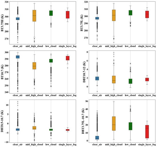
Figure 6. Distribution of the four sample types under BT and BTD in different bands (using 2019 as an example). The subplots display BT at 3.75H μm, 3.75L μm, and 10.7 μm, and BTD for 10.7–12.0 μm, 8.5–10.7 μm, and 3.75L–10.7 μm. All values are presented in Kelvin (K). The statistical notation of the boxplots (including the median, IQR, whiskers, and outliers) is defined as in Figure 5.

The 10.7 μm band, located within an atmospheric window, is primarily influenced by CO₂ absorption bands and is less affected by other non-dominant atmospheric gases (e.g., water vapor and ozone). As a result, the BT data received at 10.7 μm predominantly comes from thermal radiation emitted by target objects such as clouds and fog [37]. Therefore, 10.7 μm BT is commonly used to estimate cloud top height. In clear air regions, with no cloud cover and a well-defined vertical atmospheric structure, radiation received by the sensor mainly originates from the Earth’s surface, leading to higher BT values. In contrast, cloud-covered areas, especially those with mid-high cloud, exhibit lower BT values due to the colder temperatures at the cloud tops. This inverse relationship between BT and cloud top height supports the findings in Figure 6, where clear air samples show the highest BT, followed by sea fog and low cloud, with mid-high cloud having the lowest values.

The variation in brightness temperature difference primarily reflects the differing absorption characteristics and phase states of ice crystals and water droplets. Most low clouds and sea fog consist of water droplets, with some low clouds potentially containing a mixture of water droplets and ice crystals. Mid-high clouds, on the other hand, are composed of ice crystals [38], which account for the higher brightness temperature differences observed in mid-high clouds compared to other cloud types.

3.1.3. Texture Characteristics

Sea fog in the South China Sea is primarily advective fog, characterized by sea surface air temperatures exceeding SST. This occurs through eddy diffusion, where warm, moisture-saturated air from upper layers is transported to the cooler sea surface [39]. Compared to other cloud types, sea fog exhibits more uniform and smoother textural characteristics, which manifest as lower BT variability in the BT channel. In this study, the 10.7 μm channel within the atmospheric window is used to explore thermal radiation differences between cloud and fog targets, thereby assessing textural smoothness [4].

To further illustrate these textural differences, Figure 7 shows the standard deviation of BT at 10.7 μm (STD BT10.7) within 2 × 2 spatial grid cells for sea fog, clear air, and other cloud types. Given that the spatial resolution of each grid cell in the FY-4 satellite is 4 km, this study examines the textural variations of cloud and fog features within a 64 km spatial range. The distribution indicates that the standard deviation of BT for sea fog is much lower than that of mid-high cloud. Furthermore, sea fog data predominantly fall within a lower standard deviation range compared to other cloud systems, suggesting that thermal radiation in sea fog remains relatively stable within a 64 km spatial range, with highly uniform texture. In contrast, other cloud types exhibit greater variability and irregularity in texture, providing a useful criterion for distinguishing sea fog from other clouds.

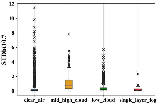
Figure 7. Distribution of the standard deviation of BT at 10.7 μm for the four sample types (using 2019 as an example). The statistical notation of the boxplots (including the median, IQR, whiskers, and outliers) is defined as in Figure 5.

3.1.4. Auxiliary Parameters

The Normalized Difference Snow Index (NDSI) distinguishes snow cover from other land surfaces by measuring reflectance in the visible and shortwave infrared bands [40]. Mid-high clouds, which are typically composed of ice crystals due to their higher altitudes, exhibit spectral characteristics similar to those of snow [41]. Due to scattering effects, mid-high clouds have higher reflectance in the visible spectrum than other cloud types, making them appear brighter in true-color imagery, while they show lower reflectance in the shortwave infrared band.

Based on the difference between the 0.47 μm visible reflectance and 2.25 μm near-infrared reflectance of the target, clear air samples exhibit the highest NDSI distribution and median values. Mid-high clouds have a relatively high median, while low clouds and sea fog exhibit similar medians, as shown in Figure 8. The NDSI calculation formula is as follows:

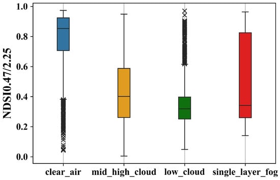
Figure 8. Distribution of NDSI for the four sample types (using 2019 as an example). The statistical notation of the boxplots (including the median, IQR, whiskers, and outliers) is defined as in Figure 5.

Based on the characteristic difference between the 0.47 μm visible reflectance (R0.47) and 2.25 μm shortwave infrared reflectance (R2.25), the NDSI provides a powerful criterion for cloud phase discrimination. In this study, clear air samples exhibit the highest NDSI distribution and median values, followed by mid-high clouds, while liquid-phase low clouds and sea fog exhibit similar, lower medians (Figure 8). Following the established index definitions for ice-phase characterization [40], the NDSI is calculated as follows:

$$\mathrm{NDSI}={\displaystyle \frac{\mathrm{R}0.47-\mathrm{R}2.25}{\mathrm{R}0.47+\mathrm{R}2.25}}$$

(7)

As thermal infrared channels primarily receive radiant energy from the emissions of target objects, and the emissivity of clouds and fog in the longwave infrared window (10.7 μm) is approximately 1, observations from this channel are highly effective for estimating the cloud/fog top temperature. Due to the vertical temperature gradient in the troposphere, the BT at 10.7 μm (BT10.7) typically decreases as the cloud top altitude increases. Following the methodology of Garand [42], which defines cloud height features based on the temperature contrast between the cloud top and the underlying surface, the cloud/fog top height (H) can be estimated using the SST and the observed BT10.7. By applying the standard atmospheric lapse rate, γ = 0.65 °C/(100 m) (indicating a temperature decrease of 0.65 °C for every 100 m increase in altitude), the target altitude is determined by the difference between the cloud top BT10.7 and the corresponding clear-air SST of the underlying layer. The calculation formula for the fog top height is as follows:

$$\mathrm{H}={\displaystyle \frac{\mathrm{SST}-\mathrm{BT}10.7}{0.65}}\times 100\mathrm{m}$$

(8)

Obtaining BT data for clear air sea surfaces under cloud cover is challenging. Therefore, this study employs ERA5 reanalysis data to derive SST along the CALIPSO scan tracks. As shown in Figure 9, under clear air conditions, the radiant energy received by the 10.7 μm channel primarily comes from terrestrial thermal radiation, which is substantial and minimally influenced by cloud cover. This results in a relatively high median position in the box plot, with a concentrated data distribution. In contrast, the impact of sea fog and other cloud systems on the 10.7 μm BT primarily originates from the fog/cloud top rather than the land surface. This leads to a reduction in the temperature difference value (BT10.7–SST), with the reduction being smallest in sea fog, followed by low cloud, and mid-high cloud. Among these, mid-high clouds exhibit the lowest average BT10.7–SST value, reaching approximately −30 °C, which aligns with the physical principle that BT decreases with increasing cloud top height.

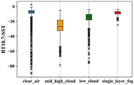
Figure 9. Distribution of the temperature difference between BT at 10.7 μm and SST for the four sample types (using 2019 as an example). The statistical notation of the boxplots (including the median, IQR, whiskers, and outliers) is defined as in Figure 5.

3.2. Analysis of Key Parameters in the Physical Mechanism

Sea fog in the South China Sea primarily consists of advection-cooled fog, and its formation is closely linked to favorable wind direction and speed, a stable atmospheric structure maintained by temperature inversions, and high relative humidity [8,14,43]. This study examines key physical quantities related to sea fog formation, including meridional and zonal wind components at 10 m height, air temperature at various vertical layers, and relative humidity. The statistical distribution of wind, temperature inversion, and humidity are reflected in Figure 10.

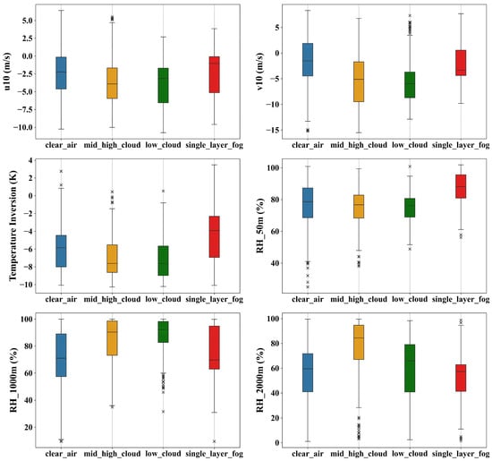
Figure 10. Distribution of the four sample types under various physical mechanism parameters (using 2022 as an example). The subplots display the zonal wind (u10) and meridional wind (v10) components at 10 m, temperature inversion strength, and relative humidity (RH) at 50 m, 1000 m, and 2000 m. The statistical notation of the boxplots (including the median, IQR, whiskers, and outliers) is defined as in Figure 5.

During the formation and maintenance of sea fog, wind speeds are generally low, typically under 4 m/s, facilitating heat exchange between warm, moist air and the cold sea surface, which leads to fog formation [14]. From the 10 m zonal and meridional wind fields, the median zonal wind of sea fog is about −1 m s⁻¹ (easterly), and the median meridional wind is about −2.5 m s⁻¹ (northerly). The zonal wind of sea fog is weaker than that of clear air, while its meridional wind is stronger. Overall, the wind speed of sea fog is lower than that of other cloud systems, consistent with the conditions for sea-fog formation and maintenance.

The presence of a temperature inversion layer is another critical factor. The inversion confines water vapor within a specific vertical range, creating a stable cold atmospheric layer that reduces turbulent mixing. This enhances heat exchange between warm, moist air and the cold sea surface, thereby promoting the formation and persistence of sea fog. For example, sea fog along the US West Coast is characterized by a strong inversion within the boundary layer [16].

In the South China Sea, sea fog is typically shallow, and the base of the capping inversion is frequently observed within the lower few hundred meters (approximately 180–400 m). In some warm-advection cases, fog may interact with overlying stratus, and the cloudy layer can deepen to exceed 1000 m [23,39,44]. Given these characteristics and the available vertical nodes in the auxiliary meteorological profiles, we quantify inversion strength using the temperature contrast between 1000 m and 50 m, defined as T1000m−T50m. This metric serves as an effective proxy for lower-tropospheric stability relevant to fog maintenance: stronger positive values indicate a more stable stratification with weaker lapse rates, which limits vertical moisture transport and helps sustain the shallow fog layer. In our dataset, sea fog exhibits markedly stronger inversion strength than low cloud, mid–high cloud, and clear-air conditions, consistent with a more stable near-surface structure that inhibits vertical mixing and moisture dilution.

Water vapor, represented by relative humidity (RH), also plays a key role in sea fog development. Higher relative humidity favors fog formation [14], particularly under stable boundary-layer conditions. Importantly, the vertical structure of RH, rather than a single-level value, provides discriminative information for separating sea fog from stratiform clouds. Previous studies have demonstrated that the vertical RH gradient is an effective discriminator between sea fog and low stratus, with sea fog typically exhibiting very high near-surface RH and a rapid decrease with height, while stratus tends to show a relatively higher RH maximum aloft (e.g., around ~1 km) [8]. In this study, RH_50m serves as the representative variable for near-surface humidity. Observations indicate that at 50 m, single-layer fog has a higher relative humidity, with median relative humidity values above 85%, which is conducive to sea fog formation. At 1000 m, the relative humidity of sea fog begins to decrease, while that of low cloud increases. At 2000 m, both sea fog and low cloud exhibit reduced relative humidity, consistent with the structural characteristics of sea fog, which typically has a thickness of about 300–400 m and a relatively low fog-top altitude [23]. However, medium and high clouds mostly have high relative humidity at 2000 m.

3.3. Validity of the Transfer Model

To verify the effectiveness of the radiometric transfer model in mitigating domain shifts between sensors, we constructed a representative independent test set (N = 264) covering different mission stages. Specifically, we selected samples from 2019 (early FY-4A phase) and 2022 (late FY-4A phase) together with 2023 (January–April, FY-4B initial operational phase) to rigorously evaluate the transfer capability across varying instrument states. The 21-dimensional feature matrix (detailed in Section 2.3.3) served as the input.

Table 7 presents a comparative evaluation of the DT, RF, and SVM models under two experimental settings: the pre-migration baseline (using native FY-4B radiances directly) and the post-migration framework (using FY-4B radiances transferred to the FY-4A). The results demonstrate that the radiometric transfer significantly improves detection performance across most categories (clear air, low cloud, and sea fog). For the sea fog category, POD increased from 0.74 to 0.77 for DT, from 0.62 to 0.73 for RF, and from 0.71 to 0.73 for SVM. The F1-score increased from 0.70 to 0.74 for DT, from 0.71 to 0.79 for RF, and from 0.73 to 0.77 for SVM. A slight decrease was observed for mid-high cloud, likely because the transfer model primarily emphasizes surface-related radiometric features and lacks sufficient representation of upper-level cloud characteristics above approximately 2 km (detailed discussion in Section 4.1). Taken together, the results support the practical value of a radiometric transfer framework that combines machine learning with physical constraints for sea fog detection over the South China Sea.

Table 7. Comparative performance of machine learning models before (Native) and after (Transferred) applying the radiometric transfer model. The “Transferred” metrics correspond to the operational FY-4B sea fog detection framework. The evaluation is based on an independent test set of 264 samples.

Target Types	Metric	DT (Native)	DT (Transferred)	RF (Native)	RF (Transferred)	SVM (Native)	SVM (Transferred)
Sea Fog	POD	0.74	0.77	0.62	0.73	0.71	0.73
	F1-score	0.70	0.74	0.71	0.79	0.73	0.77
Clear Air	F1-score	0.77	0.86	0.91	0.93	0.83	0.86
Low Cloud	F1-score	0.72	0.84	0.84	0.92	0.80	0.91
Mid-high Cloud	F1-score	0.90	0.83	0.94	0.91	0.87	0.86
Overall	Accuracy	0.77	0.82	0.86	0.89	0.81	0.85

3.4. Features Optimization and Ablation Experiment

To assess individual feature contributions and handle potential redundancy among correlated spectral channels, we conducted a group-wise ablation analysis and a Sequential Forward Selection (SFS) using the fixed stratified train–test split spanning the period from 2019 to 2023. The baseline model (“Baseline (All)”) refers to the RF trained with the complete 21-feature set, including: (i) optical reflectance bands (ref0.47, ref0.65, ref0.825, ref1.61, ref2.25), (ii) thermal infrared brightness temperatures (bt10.7, bt3.75H, bt3.75L), (iii) brightness temperature differences (DBT10.7–12, DBT8.5–10.7, DBT3.75L–10.7), (iv) derived indices (NDSI0.47/2.25, STDbt10.7, BT10.7–SST), (v) physical-mechanism parameters (surface_wind_speeds_10m_u, surface_wind_speeds_10m_v, temperature_inversion, RH_50m, RH_1000m, RH_2000m), and (vi) the Year variable.

The group-wise ablation results (Table 8) illustrate how different feature groups influence detection performance. Removing the physical-mechanism (meteorological) parameters leads to the largest degradation, confirming that these variables provide the primary physical constraints by characterizing advection (10 m wind components), boundary-layer stability (temperature inversion), and near-surface moisture structure (multi-level RH). In quantitative terms, the absence of this group reduces Fog-F1 from 0.8440 to 0.7619 (ΔFog-F1 = −0.0821), accompanied by a substantial drop in Fog-Recall (0.7881 to 0.6887; ΔRecall = −0.0993), Fog-CSI (0.7301 to 0.6154; ΔCSI = −0.1147), and Macro-F1 (0.9044 to 0.8461; ΔMacro-F1 = −0.0583).

Table 8. Group-wise ablation results (leave-one-group-out) of the Random Forest model using a fixed stratified train–test split (2019–2023). Metrics are reported for single-layer sea fog recall, F1-score, CSI, and the global macro-average F1-score; Δ denotes the change relative to the baseline model using all 21 features.

Experiment	Fog Recall	ΔRecall	Fog F1	ΔFog F1	Fog CSI	ΔFog CSI	Macro-F1	ΔMacro-F1
Baseline (All)	0.7881	0.0000	0.8440	0.0000	0.7301	0.0000	0.9044	0.0000
Remove Ref	0.8013	0.0132	0.8259	−0.0180	0.7035	−0.0266	0.8933	−0.0111
Remove BT	0.8079	0.0199	0.8472	−0.0066	0.7349	0.0049	0.9066	0.0023
Remove BT_Dif	0.7815	−0.0066	0.8399	−0.0041	0.7239	−0.0061	0.9027	−0.0017
Remove Meteorology	0.6887	−0.0993	0.7619	−0.0821	0.6154	−0.1147	0.8461	−0.0583
Remove Indices	0.7815	−0.0066	0.8339	−0.0100	0.7152	−0.0149	0.9042	−0.0002
Remove Year	0.7881	0.0000	0.8410	−0.0030	0.7256	−0.0045	0.9076	0.0033

By contrast, removing optical reflectance increases Fog-Recall slightly (ΔRecall = +0.0132) but decreases Fog-F1 (ΔFog-F1 = −0.0180), indicating that reflectance cues mainly help suppress false alarms and improve precision. Removing BT (absolute brightness temperatures) yields small improvements in Fog-Recall (ΔRecall = +0.0199) and Fog-CSI (ΔCSI = +0.0049) with negligible change in Fog-F1 (ΔFog-F1 = −0.0066) and a slight gain in Macro-F1 (ΔMacro-F1 = +0.0023), suggesting complementary information that is partly redundant with other spectral/thermal predictors. In contrast, removing BT-difference features or indices causes small but consistent declines in Fog-F1 and Fog-CSI, implying that these derived variables contribute additional discriminative power beyond raw BT/reflectance alone. Finally, removing Year produces only marginal changes, indicating that temporal information provides limited incremental benefit for this dataset under the current sampling strategy.

Given these outcomes and the goal of reducing spectral redundancy, we further performed a within-group refinement using SFS with the six meteorological parameters fixed as a baseline. A feature was retained only if it improved Sea Fog F1, CSI, or Macro F1 by >0.1%. This process yielded a compact subset of seven representative predictors: ref0.65, bt10.7, BT10.7–SST, ref1.61, DBT8.5–10.7, ref2.25, and STDbt10.7. Evaluations using the same RF configuration confirm that the SFS-refined feature set improves both fog detection sensitivity and overall balance. Specifically, fog recall increases by 2%, fog F1 increases by 1.5%, and fog CSI increases by 2.3%, while macro-average F1 also improves by 0.69% (Table 9), outperforming the full 21-feature baseline. Based on these results, the SFS-refined 13-feature configuration is adopted as the main feature set for subsequent model comparisons.

Table 9. Performance of the SFS-refined feature set (13 features) compared with the full 21-feature baseline, evaluated with the same fixed stratified train–test split as in Table 8.

Model	Features	Fog F1	Fog Recall	Fog CSI	Macro-F1
Baseline (All)	All 21 features	0.8440	0.7881	0.7301	0.9044
SFS-refined	13 features (6 meteo + 7 spectral/thermal) *	0.8592	0.8079	0.7531	0.9113

* The SFS-refined 13-feature set consists of: Meteorology (fixed): surface_wind_speeds_10m_u, surface_wind_speeds_10m_v, temperature_inversion, RH_50m, RH_1000m, RH_2000m; Spectral/thermal (selected): ref0.65, bt10.7, BT10.7–SST, ref1.61, DBT8.5–10.7, ref2.25, and STDbt10.7.

To better understand the decision logic of the optimized model, we analyzed the permutation importance for the SFS-refined 13-feature RF model based on Fog F1 (Figure 11). The results show that ref0.65 provides the largest contribution, indicating that visible reflectance is a key discriminator for fog and cloud/clear air scenes through their distinct optical thickness and scattering characteristics. Thermal variables also play an important role. BT10.7 and the temperature contrast term BT10.7 minus SST quantify the relationship between cloud top brightness temperature and the underlying sea surface, which is physically consistent with the near-surface and shallow nature of sea fog layers and helps separate surface-attached fog from elevated clouds. The contribution of ref2.25 further supports the utility of shortwave infrared sensitivity to droplet size and liquid water content for distinguishing fog from higher cloud types.

Figure 11. Permutation feature importance of the SFS-refined 13-feature Random Forest model evaluated with Fog-F1. Each bar shows the mean decrease in Fog-F1 after randomly permuting a single predictor on the held-out test set; error bars denote the standard deviation across permutation repeats. Larger decreases indicate stronger contributions to overall multi-class discrimination.

Meteorological variables, including multi-level relative humidity and temperature inversion, especially RH_1000m, act as the fundamental signal for object detection, which shows the importance of vertical humidity stratification and thermodynamic stability in distinguishing sea fog. Horizontal wind characteristics together with other physical variables show moderate but consistent importance, reflecting that they mainly constrain the classification to physically plausible environments for fog occurrence. It is worth noting that permutation importance measures the marginal contribution of individual variables, whereas the group-wise ablation captures the joint impact. The ablation results reveal physical mechanism parameters primarily through their mutual interactions to impose environmental constraints on sea fog formation, rather than acting as independent predictors. This explains why individual meteorological features appear less dominant in the permutation ranking. For completeness, we also report the Random Forest impurity-based feature importance in Appendix A.

3.5. Performance Comparison of Machine Learning Models

Based on the SFS-refined 13-feature subset and optimized hyperparameters (RF: n_estimators = 340; SVM: C = 57.1, Gamma = 0.65; DT: max_depth = 14), Table 10 presents the final comparative evaluation. With the optimized configuration applied, RF achieved the highest overall accuracy at 0.91, followed by SVM at 0.87 and DT at 0.86. This pattern is consistent with the ensemble advantage of RF in handling complex spectral-physical interactions. For the clear air category, RF performed best with an F1-score of 0.92, while DT and SVM obtained 0.88 and 0.84, respectively. For low cloud, both RF and SVM maintained strong recognition performance, reaching F1-scores of 0.93 and 0.92, while DT remained lower at 0.88. For mid-high cloud, RF and SVM yielded comparable F1-scores of 0.94, outperforming DT (0.90).

Table 10. Performance comparison of the three machine learning models using the optimized SFS-13 feature subset with the radiometric transfer model applied.

Target Types	Decision Tree (DT)			Random Forest (RF)			Support Vector Machine (SVM)
	Precision	Recall	F1-Score	Precision	Recall	F1-Score	Precision	Recall	F1-Score
Clear air	0.87	0.89	0.88	0.89	0.95	0.92	0.87	0.81	0.84
Low cloud	0.87	0.89	0.88	0.93	0.93	0.93	0.93	0.91	0.92
Mid-high cloud	0.89	0.91	0.90	0.92	0.95	0.94	0.90	0.97	0.94
Sea fog	0.79	0.74	0.76	0.90	0.81	0.85	0.79	0.80	0.80
Accuracy	0.86			0.91			0.87
Train Set Size	Total: 2416 (604/class)			Test Set Size			Total: 604 (151/class)

For the sea fog category over the South China Sea, all three models showed different detection abilities. The F1 scores for sea fog were 0.76 (DT), 0.85 (RF), and 0.80 (SVM), with POD (Recall) of 0.74 (DT), 0.81 (RF), and 0.80 (SVM), respectively. The RF model exhibited the highest performance in both precision (0.90) and recall, indicating it successfully detected the majority of sea fog events while effectively minimizing false alarms. However, the F1-score of sea fog was slightly lower than for the other classes, which reflects the more complex radiative and physical characteristics of sea fog.

Comparative evaluation of sea-fog detection studies provides insight into how regional environments, satellite sensors, and labeling strategies influence model performance. Significant variability exists among regions due to atmospheric and oceanic conditions, fog morphology, and differences in validation methodology. Representative studies and their performance metrics are summarized in Table 11. Comparative evaluation indicates that the optimized RF model offers improved detection capabilities for the South China Sea. Specifically, relative to existing studies in this region (POD 0.71–0.76), our model achieved a POD of 0.81 and an F1-score of 0.85. However, it is important to acknowledge that this performance still presents a notable gap compared to the advanced benchmarks achieved in the Yellow and Bohai Seas (where PODs can reach 0.94). This disparity is largely attributed to the greater environmental challenges in our study area compared to the northern seas.

Table 11. Summary of representative studies on satellite-based sea fog detection.

Author (Ref.)	Study Area	Satellite/Resolution	Label Extraction	Method	Validation Approach	Performance
Wang et al. [20]	Bohai and East China Seas	FY-3D/1 km	CALIOP	DT, SVM, KNN, NN	Model test set	DT:POD = 0.88;
						SVM:POD = 0.938
						KNN:POD = 0.924;
						NN:POD = 0.934;
Kim et al. [10]	Yellow Sea	GOCI + Himawari-8/500 m	Stations	DT	Site-based validation	FAR = 0.33;
						POD = 0.66;
						Accuracy = 0.67
Zhou et al. [45]	Yellow Sea	GOCI/500 m	NSMC fog product	Dual-branch neural network	Model test set	F1 = 0.77;
						CSI = 0.63
Fu et al. [12]	Arctic Ocean	MODIS/1 km	CALIOP	RF, SVM	Model test set	RF:POD = 0.735; SVM:POD = 0.708
Geng et al. [46]	East China Sea	FY-4A/4 km	Stations	Thresholding	Site-based validation	POD = 0.698;
						CSI = 0.589;
						FAR = 0.212
Zhang et al. [47]	Taiwan Strait	FY-2E/5 km	Stations	Thresholding	Site-based validation	POD = 0.71;
						FAR = 0.165;
						MDR = 0.29
Zhang et al. [48]	South China Sea	FY-4A/4 km	/	Thresholding	Site-based validation	POD = 0.76

Fog characteristics differ substantially between the two regions: Yellow and Bohai Sea fog events occur more frequently, persist longer, and form extensive, continuous layers, which makes them easier for satellites to identify. In contrast, fog over the South China Sea tends to be fragmented, small-scale, and short-lived, posing greater difficulty for satellite-based retrieval. Furthermore, differences in satellite sensors affect performance evaluation: polar-orbiting satellites generally provide higher observational accuracy due to finer spatial resolution, whereas geostationary satellites such as FY-4A/B offer higher temporal coverage but coarser resolution (4 km), leading to slightly reduced detection precision.

It is also important to note that variations in ground-truth extraction and validation methods contribute to discrepancies among studies. For instance, sea-fog labels derived from ground-station visibility records are typically validated using the same type of station data, while those extracted from CALIOP active-lidar observations are verified using CALIOP. CALIOP-based labels usually represent single-layer fog or cloud, whereas station-based labels do not distinguish vertical structure, which can further influence accuracy metrics.

Overall, the validation results demonstrate that the FY-4B geostationary satellite effectively fills the observational gap in sea-fog monitoring over the South China Sea, providing slightly improved performance compared with FY-4A. These findings confirm the potential of FY-4B multi-source fusion with physical-mechanism parameters and machine learning optimization for operational, high-resolution sea-fog detection in this region.

To evaluate the classification performance of each model, confusion matrices were constructed for the three machine learning algorithms, as shown in Figure 12. During the classification of single-layer fog, all models predominantly misclassified it as either clear air or low cloud. The RF model correctly classified 122 instances of single-layer fog, misclassifying 17 as clear air, 6 as mid-high cloud, and 6 as low cloud, resulting in a recall of 0.81. The 17 instances misclassified as clear air likely correspond to optically thin fog or fragmented fog edges. In these scenarios, the satellite sensor receives significant signal contributions from the underlying dark ocean surface, causing the spectral signature to resemble clear-sky water rather than a bright fog layer.

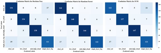
Figure 12. Confusion matrices for each machine learning model (with 151 samples per category).

Although the spectral characteristics of low cloud and sea fog are very similar, all three models misclassified fewer than or equal to 8 of the 151 low cloud test samples as sea fog. Additionally, the RF and SVM models misclassified only 6 and 5 fog samples as low cloud, respectively. This suggests that the introduction of physical constraints (e.g., BT10.7–SST and RH_1000m) contributes positively to differentiating surface-contacting fog from elevated stratus, although some spectral ambiguity inevitably persists.

It is also worth noting that while SVM achieves a comparable recall to RF, it struggles significantly with False Positives at the clear-air boundary. As shown in the confusion matrix, SVM misclassified 24 clear air samples as sea fog, whereas RF misclassified only 5. This indicates that the RF model is far more robust in correctly rejecting clear-sky scenes, maintaining high precision while ensuring sensitivity.

3.6. Case Analyses

To evaluate the operational robustness and generalization capability of the final optimized model, we retrieved sea fog cases over the South China Sea using the classifier (DT, RF, and SVM) configured with the optimal 13-feature subset determined in the ablation study (Section 3.4). Spectral features from FY-4B (2023–2025) were integrated with reanalysis for multi-source fusion retrieval. This approach was further supported by visibility data from the National Oceanic and Atmospheric Administration (NOAA, Asheville, NC, USA) Integrated Surface Dataset (ISD) (https://www.ncei.noaa.gov/metadata/geoportal/rest/metadata/item/gov.noaa.ncdc:C00532/html, accessed on 19 May 2025) and auxiliary assessments from visibility monitoring stations in Zhanjiang, China. Figure 13 illustrates the retrieval results of three representative sea-fog cases over the South China Sea. In this region, sea fog generally forms when near-surface visibility drops below 1 km. However, because most coastal ground observation stations are located some distance inland from the shoreline, the visibility threshold used to identify sea fog can be appropriately relaxed in practice.

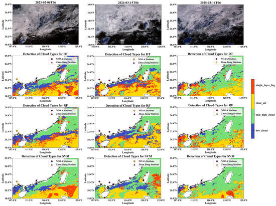
Figure 13. Sea fog retrieval results using the optimized Random Forest model (with the selected feature subset) in the South China Sea for 2023, 2024, and 2025. In the legend at the top right corner, circular labels represent NOAA stations in the region for the respective time, and triangular labels indicate the Zhanjiang station. Station colors denote visibility conditions: gray for visibility ≥ 5 km, purple for visibility between 3 km and 5 km, yellow for visibility between 2 km and 3 km, orange for visibility between 1 km and 2 km, and red for visibility < 1 km.

On 14 March 2025, sea fog with visibility below 1 km occurred near Zhanjiang, with the Beibu Gulf region experiencing visibility below 5 km. Satellite imagery showed thin cloud cover with a dark hue and uniform texture, with some areas of the sea surface faintly visible. The DT, RF, and SVM models all successfully identified sea fog in the Beibu Gulf area. For the coastal sea fog near Zhanjiang, DT and RF achieved effective detection, while the SVM labeled the core as low cloud but successfully identified sea fog along the surrounding cloud edges.

On 15 March 2024, and 6 February 2023, coastal Zhanjiang again experienced sea fog with visibility below 1 km. In the 2024 case, DT and RF identified the sea fog event. Satellite imagery showed bright, fluffy clouds with a certain thickness above the fog, and DT, RF, and SVM classified portions of these clouds as low clouds. In the 2023 case, RF mostly misclassified it as low cloud but identified a small portion as sea fog, and the corresponding satellite imagery revealed sea fog surrounded by darker clouds, with a gap exposing the sea surface and thin mist. This distribution closely matched RF’s retrieval. Additionally, RF identified sea fog below low cloud in the Beibu Gulf with visibility below 1–5 km. This may reflect the potential for low cloud and sea fog to transition during formation, so sea fog beneath low cloud may have existed. The thin cloud distribution in the satellite image aligned more closely with RF’s retrieval.

In summary, the RF model demonstrated the most accurate and detailed classification of clouds, fog, and clear air, particularly excelling in distinguishing low clouds from sea fog. The DT model identified the most sea fog pixels, but their distribution was often fragmented. The SVM model exhibited the highest spatial continuity, but tended to misclassify small, dispersed sea fog patches as homogeneous areas, overlooking detailed boundaries. Under multi-layer cloud cover (e.g., mid/high clouds obscuring low clouds), all models performed less effectively in sea fog detection. However, they performed better under single-layer cloud/fog conditions.

4. Discussion

This study demonstrates the efficacy of a machine learning framework integrating cross-satellite calibration and physical constraints for daytime sea fog detection over the South China Sea. However, several challenges and future directions warrant discussion.

4.1. Model Generalization and Operational Robustness

Regional complexity poses a primary challenge to model generalization. Physical understanding of sea fog is still incomplete, and the Beibu Gulf, Qiongzhou Strait, and Taiwan Strait differ in prevailing synoptic regimes and microphysical properties. The lack of an objective, physics-based classification standard for sea fog samples from these distinct maritime areas may currently constrain the model’s generalizable discriminative power. To address this, future research needs to delve deeper into the region-specific formation mechanisms and incorporate more refined physical parameters, such as air–sea temperature difference and stability indices (lifting condensation level, vertical wind), to improve regional adaptability. Furthermore, while the current framework prioritizes the composite BT10.7–SST feature to capture the vertical thermal contrast, the role of raw SST remains fundamental and warrants sensitivity experiments under varying seasonal conditions.

Beyond regional variability, operational robustness is influenced by sample size and spatial resolution constraints. The relatively small number of sea fog samples is primarily due to the narrow swath of the CALIOP lidar and the strict screening criteria required to match the 4 km resolution of FY-4 AGRI. While the sample size is limited, the integration of physical mechanism constraints (temperature inversion, boundary layer humidity, and wind field) significantly enhances the model’s generalization capability. Unlike purely data-driven methods that rely solely on spectral textures, these physical parameters represent the universal thermodynamic conditions required for sea fog formation, ensuring robust detection even with limited training data. However, a trade-off exists regarding spatial scale; the 4 km resolution of the AGRI sensor limits the detection of fragmented or small-scale sea fog patches. Techniques such as super-resolution or downscaling offer potential pathways to better capture these fine-scale events.

Another significant detection barrier arises from the inherent limitation of passive remote sensing to penetrate thick cloud layers. Our case analyses confirm that under multi-layer, thick-cloud conditions, the satellite’s spectral signal is dominated by the radiative properties of the uppermost cloud layers. This vertical limitation also constrains the applicability of ground-based quantitative validation. While coastal stations and buoys provide reliable surface visibility records, they cannot characterize the atmospheric structure above the fog. In ‘fog-under-cloud’ scenarios, a station reports fog, but the satellite sensor captures the upper cloud signal. Validating against such data without vertical profiling would introduce discrepancies where the model is penalized for correctly identifying the upper cloud layer, contradicting our training focus on single-layer detection. Consequently, model performance is superior under single-layer or thin-cloud conditions. Future research should focus on quantifying the radiative differences between overlapping cloud layers and underlying fog to enhance detection capability within complex cloud systems.

Finally, advanced deep learning is a powerful technique for improving sea fog detection accuracy. Architectures such as U-Net, C-GAN, or other hybrid models can capture more multiscale spatial context and texture. Building on the effectiveness of the transfer model to address the data continuity challenge after CALIOP data ended in 2023, our subsequent research will extend the current along-track labels into spatial annotations. This will allow for a systematic comparison of sea fog identification accuracy using various deep learning architectures. The ultimate objective is to operationalize a robust FY-4B sea fog monitoring product that provides high-resolution support for fog events over the South China Sea.

4.2. Radiometric Transfer Model

The slight decline in mid-high cloud classification accuracy following the radiometric transfer can be attributed to complex radiative interactions that are challenging for a global empirical transfer model to fully capture.

Physically, mid-high clouds exhibit complex interactions with solar and thermal radiation, including multi-layer scattering, variable optical depths, and phase-dependent (ice vs. liquid) absorption/emission properties [2,38]. Unlike liquid droplets, ice crystals in high clouds are non-spherical, inducing complex scattering phase functions that create non-linear spectral signatures [49]. In our MODTRAN-based simulations, while typical cloud parameters were incorporated, the model’s reliance on global empirical fitting tends to smooth over these localized non-linearities.

Radiometrically, as noted in satellite intercalibration studies, the Spectral Band Adjustment Factor is highly dependent on the target’s spectral signature [50]. Our MODTRAN simulations prioritized surface and low-level diversity to ensure global robustness, which minimizes the overall error across diverse surface types (e.g., ocean, land), and often fails to capture the specific spectral shifts caused by the complex microphysics of high-altitude ice clouds. Specifically, high clouds like cirrus often possess semi-transparent properties, leading to the partial transmission of underlying surface radiation [37]. This introduces significant variability in the simulated radiance that, when convolved with sensor-specific Spectral Response Functions, amplifies discrepancies in brightness temperatures.

To address these limitations, our future work will focus on integrating advanced cloud microphysics from models like RTTOV and developing scene-adaptive transfer functions that dynamically adjust coefficients based on cloud types.

5. Conclusions

This study addresses the operational and continuous monitoring needs for daytime sea fog in the South China Sea by proposing a novel machine learning framework for sea fog identification using FY-4A/FY-4B data. The framework integrates cross-satellite radiometric calibration with physical mechanism constraints, enabling data transferability through FY-4A/4B AGRI cross-satellite radiative transfer. A consistent 21-dimensional matrix of observation samples for four target categories was constructed using CALIOP, FY-4, and ERA5 data. Through ablation experiments and Sequential Forward Selection, an optimal 13-feature subset was identified. Machine learning parameters were then optimized using grid search and PSO algorithms, resulting in DT, RF, and SVM sea fog recognition models. Test set validation showed that RF achieved optimal overall performance (Accuracy: 0.91, Sea Fog F1-score: 0.85, POD: 0.81). The model’s performance exceeded existing South China Sea studies (POD: 0.71–0.76). Multi-temporal case studies using NOAA ISD and Zhanjiang visibility stations further validated the robustness and operational applicability of the FY-4B sea fog detection method. Key conclusions are as follows:

(1)

Based on a radiometric recalibration transfer model, consistency between FY-4A and FY-4B AGRI radiometric channel data has been achieved. Following radiometric recalibration, FY-4B data were converted to match the radiometric characteristics of FY-4A channels, establishing a joint spectral dataset for FY-4A/B spanning 2019 to 2025. After the migration, for sea fog, the POD of the DT model increased from 0.74 to 0.77, the RF model from 0.62 to 0.73, and the SVM model from 0.71 to 0.73, demonstrating the feasibility and effectiveness of the radiometric transfer.

(2)

Quantitative analysis of spectral sensitivity for FY-4A/B satellites indicates that visible–near-infrared reflectance (e.g., 0.65 μm) effectively distinguishes clear air from clouds/fog. The 10.7 μm band, situated within an atmospheric window, exhibits the highest sensitivity to cloud/fog-top temperatures. BT10.7 and BT10.7–SST serve as core factors for distinguishing fog, low cloud, and mid-high cloud. Multi-channel brightness-temperature differences (DBT8.5–10.7) reflect fog phase state and particle-size variations. These conclusions form the experimental basis for spectral-dimension selection in sea fog identification using FY-4A/B.

(3)

Under the physical mechanisms governing South China Sea fog formation, spectral and textural feature analyses were conducted for clear air, high clouds, low cloud, and sea fog. Results indicate that temperature inversion strength (ΔT{1000–50 m}), stratified relative-humidity gradients, and near-surface winds constitute key background conditions for the formation and persistence of advection-cooled fog, significantly enhancing fog and low-cloud distinguishability. Additionally, fog exhibits low spatial variability at 10.7 μm, with the 2 × 2 pixel STD BT10.7 metric characterizing their “smooth, uniform” texture features, effectively complementing low-cloud/thick-cloud formation.

(4)

Through grid search and PSO methods optimized in 10-fold cross-validation for RF, SVM, and DT models, results indicate that RF delivers optimal overall performance (Accuracy: 0.91; sea fog F1-score: 0.85; sea fog POD: 0.81), followed by SVM (Accuracy: 0.87). DT shows weaker overall accuracy (Accuracy: 0.86). The confusion matrix indicates that the primary errors stem from misclassifications at the “fog–clear air boundary” and between “fog and thin-layer cloud”. The proposed method improves the POD to 0.81, surpassing the 0.71–0.76 range reported in existing studies on South China Sea fog.

(5)

Multiple case studies comparing the identification of sea fog in the South China Sea for FY-4B (2023–2025) against NOAA ISD and Zhanjiang visibility station observations demonstrate that RF effectively reproduces sea fog boundaries and spatial morphology. DT exhibits higher detection sensitivity but yields spatial fragmentation, whereas SVM maintains good connectivity with slightly blunted boundaries.

References

- World Meteorological Organization. International Meteorological Vocabulary, 2nd ed.; WMO: Geneva, Switzerland, 1992; p. 248. [Google Scholar]
- Hunt, G.E. Radiative Properties of Terrestrial Clouds at Visible and Infra-Red Thermal Window Wavelengths. Q. J. R. Meteorol. Soc. 1973, 99, 346–369. [Google Scholar] [CrossRef]
- Bendix, J. A 10-Years Fog Climatology of Germany and the Alpine Region Based on Satellite Data-Preliminary Results. In Proceedings of the Second International Conference on Fog and Fog Collection, St. John’s, NL, Canada, 15–20 July 2001; pp. 357–360. [Google Scholar]
- Wu, X.; Li, S. Automatic Sea Fog Detection over Chinese Adjacent Oceans Using Terra/MODIS Data. Int. J. Remote Sens. 2014, 35, 7430–7457. [Google Scholar] [CrossRef]
- Eyre, J.R.; Brownscombe, J.L.; Allam, R.J. Detection of Fog at Night Using Advanced Very High Resolution Radiometer (AVHRR) Imagery. Meteorol. Mag 1984, 113, 266–271. [Google Scholar]
- Badarinath, K.; Kharol, S.; Sharma, A.; Roy, P. Fog over Indo-Gangetic Plains—A Study Using Multisatellite Data and Ground Observations. IEEE J. Sel. Top. Appl. Earth Obs. Remote Sens. 2009, 2, 185–195. [Google Scholar] [CrossRef]
- Wu, D.; Lu, B.; Zhang, T.; Yan, F. A Method of Detecting Sea Fogs Using CALIOP Data and Its Application to Improve MODIS-Based Sea Fog Detection. J. Quant. Spectrosc. Radiat. Transf. 2015, 153, 88–94. [Google Scholar] [CrossRef]
- Xiao, Y.; Liu, R.; Ma, Y.; Cui, T. MERRA-2 Reanalysis-Aided Sea Fog Detection Based on CALIOP Observation over North Pacific. Remote Sens. Environ. 2023, 292, 113583. [Google Scholar] [CrossRef]
- Xiao, Y.; Zhang, J.; Cui, T.; Qin, P. Review of Sea Fog Detection from Satellite Remote Sensing Data. Mar. Sci. 2017, 41, 146–154. [Google Scholar] [CrossRef]
- Kim, D.; Park, M.-S.; Park, Y.-J.; Kim, W. Geostationary Ocean Color Imager (GOCI) Marine Fog Detection in Combination with Himawari-8 Based on the Decision Tree. Remote Sens. 2020, 12, 149. [Google Scholar] [CrossRef]
- Sim, S.; Im, J. Improved Ocean–Fog Monitoring Using Himawari-8 Geostationary Satellite Data Based on Machine Learning with SHAP-Based Model Interpretation. IEEE J. Sel. Top. Appl. Earth Obs. Remote Sens. 2023, 16, 7819–7837. [Google Scholar] [CrossRef]
- Fu, Y.; Yi, L.; Li, M.; Cheng, X. Summer Sea Fog Detection over the Arctic Ocean Based on Satellite Data Using Several Machine Learning Models. J. Mar. Meteorol. 2024, 44, 14–23. [Google Scholar] [CrossRef]
- Xu, M.; Wu, M.; Guo, J.; Zhang, C.; Wang, Y.; Ma, Z. Sea Fog Detection Based on Unsupervised Domain Adaptation. Chin. J. Aeronaut. 2022, 35, 415–425. [Google Scholar] [CrossRef]
- Liao, K.; Li, K.; Dang, H.; Lin, B.; Zhao, D.; Li, H. Process and Characteristics of Occurrence and Dissipation of Sea Fog in the West Coast of the Taiwan Strait Based on Coastal Automatic Weather Station. J. Trop. Oceanogr. 2024, 43, 79–93. [Google Scholar] [CrossRef]
- Shi, D.; Zhang, J.; Cao, Q.; Li, C.; Zhu, Y. Research on Sea Fog Diagnosis in Haizhou Bay Based on Decision Tree Algorithm. J. Meteorol. Sci. 2022, 42, 136–142. [Google Scholar] [CrossRef]
- Leipper, D.F. Fog on the U.S. West Coast: A Review. Bull. Am. Meteorol. Soc. 1994, 75, 229–240. [Google Scholar] [CrossRef]
- Jeon, J.; Kim, S.-H.; Yang, C.-S. Fundamental Research on Spring Season Daytime Sea Fog Detection Using MODIS in the Yellow Sea. Korean J. Remote Sens. 2016, 32, 339–351. [Google Scholar] [CrossRef]
- Zhang, S.; Yi, L. A Comprehensive Dynamic Threshold Algorithm for Daytime Sea Fog Retrieval over the Chinese Adjacent Seas. Pure Appl. Geophys. 2013, 170, 1931–1944. [Google Scholar] [CrossRef]
- Hao, Z.; Pan, D.; Gong, F.; Zhu, Q. Optical Radiance Characteristics of Sea Fog Based on Remote Sensing. Acta Opt. Sin. 2008, 28, 2420–2426. [Google Scholar] [CrossRef]
- Wang, Y.; Qiu, Z.; Zhao, D.; Ali, M.d.A.; Hu, C.; Zhang, Y.; Liao, K. Automatic Detection of Daytime Sea Fog Based on Supervised Classification Techniques for FY-3D Satellite. Remote Sens. 2023, 15, 2283. [Google Scholar] [CrossRef]
- Wu, X.; Li, Y.; Huang, B.; Wang, X.; Song, W. Application of Dynamic Threshold Method to Sea Fog Detection with FY-2 Satellite. J. Shandong Meteorol. 2017, 37, 31–41. [Google Scholar] [CrossRef]
- Tu, S.; Han, L.; Xu, F.; Xu, J.; Zhi, X. Research Progress on Sea Fog over South China. J. Mar. Meteorol. 2019, 39, 12–20. [Google Scholar] [CrossRef]
- Huang, H.; Zhan, G.; Liu, C.; Tu, J.; Mao, W. A Case Study of Numerical Simulation of Sea Fog on the Southern China Coast. J. Trop. Meteorol. 2015, 31, 643–654. [Google Scholar] [CrossRef]
- Zhang, W.; Li, F.; Lv, Q.; Cui, M.; Zhang, Y.; Chen, D. Comprehensive Analysis of a Sea Fog Event in Southern Coast of Fujian Based on Multi-Source Data. Meteorol. Mon. 2023, 49, 682–696. [Google Scholar] [CrossRef]
- Wu, D.; Hu, Y.; McCormick, M.P.; Yan, F. Global Cloud-Layer Distribution Statistics from 1 Year CALIPSO Lidar Observations. Int. J. Remote Sens. 2011, 32, 1269–1288. [Google Scholar] [CrossRef]
- Yu, Q.; Min, M.; Di, D.; Zhao, Y.; Li, G.; Li, J.; Wang, L.; Hu, X.; Zhang, P. Spectral-Fidelity-Preserving Recalibration of Reflective Solar Bands for MERSI-II Onboard Fengyun-3D Satellite. ISPRS J. Photogramm. Remote Sens. 2025. to be submitted. [Google Scholar]
- Quinlan, J.R. Induction of Decision Trees. Mach. Learn. 1986, 1, 81–106. [Google Scholar] [CrossRef]
- Breiman, L. Random Forests. Mach. Learn. 2001, 45, 5–32. [Google Scholar] [CrossRef]
- Cortes, C.; Vapnik, V. Support-Vector Networks. Mach. Learn. 1995, 20, 273–297. [Google Scholar] [CrossRef]
- Hensman, P.; Masko, D. The Impact of Imbalanced Training Data for Convolutional Neural Networks; Degree Project in Computer Science; KTH Royal Institute of Technology: Stockholm, Sweden, 2015. [Google Scholar]
- Schaffer, C. Selecting a Classification Method by Cross-Validation. Mach. Learn. 1993, 13, 135–143. [Google Scholar] [CrossRef]
- Bergstra, J.; Bengio, Y. Random Search for Hyper-Parameter Optimization. J. Mach. Learn. Res. 2012, 13, 281–305. [Google Scholar]
- Sudheer, C.; Maheswaran, R.; Panigrahi, B.K.; Mathur, S. A Hybrid SVM-PSO Model for Forecasting Monthly Streamflow. Neural Comput. Appl. 2014, 24, 1381–1389. [Google Scholar] [CrossRef]
- Rosa, G.J.M. The Elements of Statistical Learning: Data Mining, Inference, and Prediction. Biometrics 2010, 66, 1315. [Google Scholar] [CrossRef]
- Sokolova, M.; Lapalme, G. A Systematic Analysis of Performance Measures for Classification Tasks. Inf. Process. Manag. 2009, 45, 427–437. [Google Scholar] [CrossRef]
- Lee, T.F.; Turk, F.J.; Richardson, K. Stratus and Fog Products Using GOES-8-9 3.9-μm Data. Weather. Forecast. 1997, 12, 664–677. [Google Scholar] [CrossRef]
- Inoue, T. On the Temperature and Effective Emissivity Determination of Semi-Transparent Cirrus Clouds by Bi-Spectral Measurements in the 10 μm Window Region. J. Meteorol. Soc. Jpn. II 1985, 63, 88–99. [Google Scholar] [CrossRef]
- Thies, B.; Nauß, T.; Bendix, J. Precipitation Process and Rainfall Intensity Differentiation Using Meteosat Second Generation Spinning Enhanced Visible and Infrared Imager Data. J. Geophys. Res. Atmos. 2008, 113, D23206. [Google Scholar] [CrossRef]
- Huang, H.; Liu, H.; Jiang, W.; Huang, J.; Mao, W. Characteristics of the Boundary Layer Structure of Sea Fog on the Coast of Southern China. Adv. Atmos. Sci. 2011, 28, 1377–1389. [Google Scholar] [CrossRef]
- Dozier, J.; Painter, T.H. Multispectral and Hyperspectral Remote Sensing of Alpine Snow Properties. Annu. Rev. Earth Planet. Sci. 2004, 32, 465–494. [Google Scholar] [CrossRef]
- Wielicki, B.A.; Barkstrom, B.R.; Harrison, E.F.; Lee, R.B.; Louis Smith, G.; Cooper, J.E. Clouds and the Earth’s Radiant Energy System (CERES): An Earth Observing System Experiment. Bull. Am. Meteor. Soc. 1996, 77, 853–868. [Google Scholar] [CrossRef]
- Garand, L. Automated Recognition of Oceanic Cloud Patterns. Part I: Methodology and Application to Cloud Climatology. J. Clim. 1988, 1, 20–39. [Google Scholar] [CrossRef]
- Li, X.; Wang, F.; Zhang, X.; Chan, P.W.; Yang, Y.; Lu, C.; Gao, M. Anomalous Increase in Sea Fog Frequency along Coastal China in the Early 21st Century and the Aerosol Influence. npj Clim. Atmos. Sci. 2025, 8, 365. [Google Scholar] [CrossRef]
- Huang, H.; Liu, H.; Huang, J.; Mao, W.; Bi, X. Atmospheric Boundary Layer Structure and Turbulence during Sea Fog on the Southern China Coast. Mon. Wea. Rev. 2015, 143, 1907–1923. [Google Scholar] [CrossRef]
- Zhou, Y.; Chen, K.; Li, X. Dual-Branch Neural Network for Sea Fog Detection in Geostationary Ocean Color Imager. IEEE Trans. Geosci. Remote Sens. 2022, 60, 1–17. [Google Scholar] [CrossRef]
- Geng, D.; Liu, T.; Li, C. Research on a Daytime Sea Fog Identification Model Based on FY-4A Satellite Data and Random Forest Algorithm. Mar. Forecast. 2022, 39, 83–93. [Google Scholar] [CrossRef]
- Zhang, C.; Lin, B. Application of FY—2E Data to Remote Sensing Monitoring of Sea Fog in Fujian Coastal Region. Remote Sens. Land Resour. 2018, 30, 7–13. [Google Scholar] [CrossRef]
- Zhang, Y.; Jin, K.; Liu, Z.; Liu, H.; Yang, Y.; He, M. Remote Sensing Monitoring of Sea Fog in the South China Sea Based on FY-4 Satellite Data. Meteorol. Environ. Sci. 2024, 47, 28–35. [Google Scholar] [CrossRef]
- Yang, P.; Bi, L.; Baum, B.A.; Liou, K.-N.; Kattawar, G.W.; Mishchenko, M.I.; Cole, B. Spectrally Consistent Scattering, Absorption, and Polarization Properties of Atmospheric Ice Crystals at Wavelengths from 0.2 to 100 mm. J. Atmos. Sci. 2013, 70, 330–347. [Google Scholar] [CrossRef]
- Chander, G.; Hewison, T.J.; Fox, N.; Wu, X.; Xiong, X.; Blackwell, W.J. Overview of Intercalibration of Satellite Instruments. IEEE Trans. Geosci. Remote Sens. 2013, 51, 1056–1080. [Google Scholar] [CrossRef]
Disclaimer/Publisher’s Note: The statements, opinions and data contained in all publications are solely those of the individual author(s) and contributor(s) and not of MDPI and/or the editor(s). MDPI and/or the editor(s) disclaim responsibility for any injury to people or property resulting from any ideas, methods, instructions or products referred to in the content. |
© 2026 by the authors. Licensee MDPI, Basel, Switzerland. This article is an open access article distributed under the terms and conditions of the Creative Commons Attribution (CC BY) license.