


Highlights
What are the main findings?
- MHBA-TransUNet coordinates shallow RGB–DSM fusion and deep global–local feature interaction through SCFFM and GLAM, achieving mIoU scores of 85.15%, 88.01%, and 85.49% on Vaihingen, Potsdam, and US3D, respectively.
- A lightweight SA–CA–SA dual-stream Transformer enables intra-modal context modeling and bidirectional cross-modal interaction with substantially reduced Transformer parameter overhead.
What are the implications of the main findings?
- Coordinating shallow multimodal fusion with deep semantic–spatial interaction provides an effective strategy for RGB–DSM semantic segmentation in complex urban scenes.
- The compact multimodal Transformer provides a practical approach to balancing cross-modal representation and computational efficiency in high-resolution remote sensing applications.
Abstract
High-resolution remote sensing semantic segmentation using RGB imagery and digital surface models (DSM) remains challenging because of insufficient shallow cross-modal fusion and inadequate coordination between global semantics and local spatial information. To address these issues, we propose MHBA-TransUNet, a hybrid encoder–decoder network for RGB–DSM semantic segmentation. In the encoder, a Shallow Cross-modal Feature Fusion Module (SCFFM) progressively integrates complementary RGB and DSM features through dynamic spatial recalibration, while a lightweight dual-stream Transformer with a self-attention–cross-attention–self-attention (SA–CA–SA) configuration models intra-modal context and bidirectional cross-modal interactions. During decoding, a Global–Local Alignment Module (GLAM) combines Block-Distance Linear Attention (BDLA), feature-wise modulation, and channel reweighting to coordinate deep semantic features with shallow spatial details. Experiments on the ISPRS Vaihingen, ISPRS Potsdam, and US3D datasets achieve mIoU scores of 85.15%, 88.01%, and 85.49%, respectively, outperforming representative state-of-the-art methods. Ablation studies further verify the effectiveness and complementarity of SCFFM and GLAM, while the US3D results demonstrate stable performance across diverse urban scenes.
1. Introduction
In recent years, the rapid development of Earth observation technologies has greatly improved both the acquisition capability and the usability of high-resolution remote sensing data. Remote sensing data are inherently multimodal in nature, including, for example, visible-light optical imagery, synthetic aperture radar (SAR) imagery, and digital surface models (DSM) generated from light detection and ranging (LiDAR) measurements [1]. Data from different modalities can characterize the spectral–textural properties, three-dimensional structures, and scattering behaviors of ground objects from distinct physical mechanisms and observational perspectives, thereby providing abundant complementary information for comprehensive and accurate representation of surface features. Consequently, multimodal data fusion, by integrating such complementary information, has become a key technical support for many core tasks in geographic research, with applications covering land-use and land-cover change detection [1], high-precision land-cover mapping [2], extraction of specific targets such as buildings and roads [3], image fusion [4,5,6], change detection [7], super-resolution [8], and object detection [9,10], as well as ecological monitoring and disaster assessment [11,12].
As a fundamental pixel-level classification task, semantic segmentation aims to assign each pixel in remote sensing imagery to a predefined land-cover category and serves as the basis for the aforementioned applications. Early studies mainly relied on traditional machine learning methods, such as random forests [13], support vector machines [14], and conditional random fields [15]. However, these methods are limited in their ability to automatically extract deep and abstract discriminative semantic features, making it difficult to meet the demands of fine-grained recognition for complex objects in high-resolution remote sensing imagery. In recent years, breakthroughs in deep learning have brought revolutionary advances to remote sensing semantic segmentation. Representative methods based on convolutional neural networks (CNNs) and their extensions have significantly improved segmentation accuracy and efficiency. Early CNN-based fusion approaches [16] established end-to-end learning frameworks for multimodal data, while subsequent encoder–decoder architectures [17,18] and hybrid attention-based designs [19,20,21] further advanced automatic multi-level feature representation from large-scale remote sensing data. Nevertheless, owing to the inherently local receptive fields of CNNs [22,23], natural limitations remain in modeling long-range dependencies among pixels and capturing global contextual information, and these limitations become particularly evident when complex remote sensing scenes with strong spectral heterogeneity and intricate structures are processed.
This limitation has driven the successful adoption of Transformer architectures in computer vision. In 2020,the Vision Transformer (ViT) [24] was the first to demonstrate the great potential of a pure Transformer architecture for image recognition tasks. Compared with CNNs, Transformers, by virtue of their global attention mechanism, are able to effectively model long-range dependencies among serialized image patches and exhibit superior capability in global context modeling. In particular, early Transformer-based segmentation backbones such as TransUNet [25] and Segmenter [26] demonstrated the potential of self-attention for dense prediction, while later efficient architectures including SegFormer [27] and UNetFormer [28] further adapted the paradigm to natural and remote sensing imagery. This advantage was soon introduced into the field of semantic segmentation, leading to efficient segmentation models such as SegFormer [27] and Segmenter [26], which achieved performance surpassing that of CNN-based methods on natural images.
While remarkable success has been achieved in single-modality semantic segmentation, the limitations of single-sensor data have also become increasingly evident. Constrained by imaging mechanisms and sensor characteristics, unimodal data often suffer from inherent information gaps. For example, optical imagery is easily affected by cloud and haze occlusion and is often inadequate for distinguishing highly similar spectral features; SAR imagery is subject to geometric distortions and speckle noise; and DSM lacks spectral–textural information [2,29]. By contrast, multimodal data can compensate for these deficiencies and provide more comprehensive information support for segmentation tasks.
Therefore, how to effectively integrate the complementary information contained in multimodal remote sensing data has become a central research direction for improving semantic segmentation performance. According to the stage at which fusion is performed, existing methods can generally be categorized into early fusion, intermediate fusion, and late fusion. Early fusion usually concatenates or stacks multimodal data directly at the input level. Although this strategy is straightforward, it is often inadequate for accommodating the significant differences in statistical characteristics and noise levels across modalities [30,31]. In late fusion, each modality is processed independently and the results are combined at the decision or output level. This scheme is easy to implement, but the exploitation of deep complementary correlations across modalities remains insufficient [31]. By contrast, intermediate fusion performs interaction and integration in the feature space, thereby enabling cross-modal dependencies to be captured more flexibly; for this reason, it is widely regarded as one of the most effective fusion strategies for semantic segmentation [32,33].
However, most existing multimodal fusion models built upon Transformer backbones, such as TransFuser [34] and SwinFusion [35], perform modal interaction mainly through a unidirectional cross-attention mechanism. Under such a design, the contextual features of the target modality are likely to be suppressed or overwhelmed when information from the source modality is absorbed, while the one-way information flow further restricts the efficient transmission and adaptive fusion of bidirectional complementary information across modalities [36]. In addition, when the global semantic features captured by Transformers are fused with the local detail features extracted by CNN encoders, existing methods often rely on simple addition or concatenation, without carefully handling or adaptively aligning their inherent differences in receptive field and abstraction level [36,37]. Such coarse fusion strategies are prone to causing semantic misalignment in the feature space, so that global contextual information and local fine-grained features interfere with each other, which tends to degrade the representation of fine-grained structures and the recognition of small targets.
To address the above issues, TransUNet [25] is adopted in this study as the baseline architecture, upon which a multilayer fusion network, termed Multimodal Hybrid Bidirectional Attention TransUNet (MHBA-TransUNet), is developed for RGB–DSM remote sensing image semantic segmentation. It should be noted that, throughout this paper, the term “RGB–DSM” is used in a general sense to denote three-channel optical imagery paired with elevation data (DSM/NDSM); the specific channel configurations of each dataset are described in Section 3.1. First, to mitigate the local response misalignment that arises in the shallow feature space of multimodal data, a Shallow Cross-modal Feature Fusion Module (SCFFM) is designed. Through a dynamic spatial recalibration mechanism, the shallow fine-grained features extracted from RGB imagery and DSM by the dual-branch CNN encoder are progressively interacted and fused, thereby effectively alleviating the shallow fusion difficulties caused by differences in imaging mechanisms, occlusions, and local inconsistencies, and providing high-quality feature representations for subsequent processing. Second, to overcome the insufficient collaboration between deep global semantics and shallow local details during decoding, a Global–Local Alignment Module (GLAM) is proposed. In this module, a Block-Distance Linear Attention (BDLA) mechanism and a feature-wise linear modulation strategy are introduced. While computational complexity is kept under control, long-range dependencies and local correspondences between deep semantic features and shallow spatial details are established, enabling adaptive alignment and fusion of cross-level features and improving the representation of fine-grained structures and the recognition of small targets in complex scenes. The main contributions of this study are summarized as follows:
- 1.
- A Shallow Cross-modal Feature Fusion Module (SCFFM) is proposed, in which the progressive fusion of shallow RGB and DSM features is achieved through spatial interaction enhancement and attention-based recalibration. With this design, shallow mismatches between multimodal data can be effectively alleviated, and the representation of details in shadowed and low-texture regions can be enhanced.
- 2.
- A Global–Local Alignment Module (GLAM) is proposed, within which a Block-Distance Linear Attention (BDLA) mechanism is introduced. Through the joint use of block-wise linear mixing, local positional enhancement, and feature modulation, efficient alignment and fusion of deep global semantics and shallow local details are achieved, thereby enhancing the fine-grained detail representation and small-target recognition performance of the model.
- 3.
- Comprehensive comparative experiments and ablation studies are conducted on three remote sensing datasets, namely ISPRS Vaihingen, ISPRS Potsdam, and US3D (grss_dfc_2019) [38,39]. The results show that the proposed method outperforms a variety of representative state-of-the-art methods in terms of overall accuracy, class-wise F1 scores, and mIoU, thereby validating the effectiveness of the proposed framework.
The remainder of this paper is organized as follows. Section 2 reviews related work on unimodal and multimodal semantic segmentation. Section 3 introduces the datasets and presents the architecture of the proposed MHBA-TransUNet in detail. Section 4 describes the experimental setup, including implementation details, evaluation metrics, and compared methods. Section 5 reports the experimental results, including comparative experiments, generalization experiments, complexity analysis, ablation studies, and feature visualization. Section 6 discusses the findings, mechanism interpretation, and limitations of the proposed method. Finally, Section 7 concludes the paper.
2. Related Work
2.1. Unimodal Semantic Segmentation
In the early exploration of semantic segmentation, the Fully Convolutional Network (FCN) [40], as the first CNN-based end-to-end model, laid an important foundation for this task. However, the simplified upsampling strategy adopted in its decoder resulted in blurred boundaries and insufficient segmentation accuracy. To overcome this limitation, a key improvement was achieved by UNet [41] through its innovative encoder–decoder architecture: multiscale features are captured by the encoder through progressive downsampling, while contextual information is fused by the decoder via skip connections, thereby enabling effective recovery of spatial details. Although CNN-based methods have demonstrated robust performance in segmentation tasks, their inherent local receptive field property [22,23] restricts the ability to model global semantics and makes the handling of long-range dependencies particularly challenging.
This limitation has promoted the cross-domain adoption of Transformer architectures. In 2020, ViT [24] introduced Transformers into vision tasks for the first time, breaking the locality constraint of CNNs through sequence-based modeling. Compared with conventional CNNs, ViT has shown significant advantages in global context perception [25,26,27,28]. It has not only advanced the development of cross-modal tasks such as vision–language understanding, but has also become an important paradigm for subsequent research. Overall, unimodal methods have established mature encoder–decoder paradigms, yet the information bottleneck of single-sensor data fundamentally constrains their upper performance in complex scenes. Detail–semantic decoupling has also been explored to improve feature quality in related tasks [9].
2.2. CNN-Based Multimodal Semantic Segmentation
With the continuous advancement of Earth observation technologies, multimodal remote sensing data, such as optical imagery, multispectral data, and digital surface models (DSM), have become increasingly accessible. Prior-guided fusion strategies have proven effective for heterogeneous modality integration [4,5]. Among them, DSM provides precise height information of ground objects, which not only offers critical cues for identifying structures with height consistency, such as roads and buildings, but also significantly improves semantic segmentation accuracy owing to its naturally clear structural representation [42,43]. This advantage has stimulated extensive research on deep learning-driven multimodal fusion. Early approaches, such as ResUNet-a [44], attempted to directly stack RGB images and DSM into a four-channel input. However, such a strategy is inadequate for handling the inherent statistical heterogeneity and noise discrepancies across modalities [30,31]. To address this issue, FuseNet [16] innovatively adopted a dual-branch architecture, in which RGB and DSM data are processed in parallel during encoding, while feature fusion is performed through element-wise addition. Building upon this idea, vFuseNet [45] further introduced a multi-scale fusion mechanism, thereby significantly enhancing feature representation capability. Nevertheless, fusion schemes based on simple addition still fail to fully exploit the complementarity of multimodal features.
Subsequent studies have achieved further progress through more refined fusion mechanisms. ABCNet [33] improves segmentation efficiency by combining dual-branch context modeling with an attention mechanism, thereby balancing spatial detail preservation and semantic information aggregation. DDCM-Net [46] employs dense dilated convolutions to fuse features with different receptive fields, so that contextual representation of multiscale objects can be enhanced. MANet [47], from the perspective of multiple attention mechanisms, jointly models dependency relationships in both spatial and channel dimensions, thus improving the capture of discriminative features in complex scenes. MACU-Net [48], built upon the U-Net architecture, introduces multiscale skip connections and asymmetric convolutions to strengthen cross-level feature interaction and local structure representation. Although these methods have achieved favorable results in local detail recovery, multiscale information integration, and feature enhancement, they still rely primarily on convolutional operations at their core. As a result, their capability for modeling long-range spatial dependencies remains relatively limited, which to some extent constrains semantic segmentation performance in complex remote sensing scenes.
2.3. CNN- and Transformer-Based Multimodal Semantic Segmentation
Owing to its outstanding capability in context modeling and multimodal fusion, the Transformer architecture has gradually become a core paradigm for multimodal fusion in semantic segmentation. Under this trend, TransFuser [34] innovatively embeds multiple Transformer layers into the convolutional feature fusion stage, thereby enhancing representation capacity through dynamic modeling of cross-feature-map correlations. SwinFusion [35] goes a step further by using convolutional layers as shallow feature extractors while employing Swin Transformer [49] to build the backbone for deep feature generation, demonstrating that Transformers can replace conventional CNNs as the principal backbone in fusion tasks.
Studies in remote sensing semantic segmentation have shown that combining the local modeling capability of CNNs with the global context perception ability of Transformers has become an important direction for improving model performance. CMFGNet [43] enhances semantic associations across different modalities through cross-modal multiscale interaction and a Transformer-based fusion mechanism. MSFNet [37] progressively integrates multilevel multimodal features based on a multistage Transformer architecture, thereby improving segmentation performance on high-resolution remote sensing data. MFTransNet [36] achieves complementary representation of multimodal features by combining CNNs and Transformers. TMFNet [50] adopts a multimodal branch encoding scheme together with a Transformer-based fusion strategy, thereby strengthening the interaction among information from different sources. FTransUNet [51] further unifies the local detail modeling capability of CNNs and the global context perception ability of ViT within a multilevel multimodal fusion framework.MCFTNet [52] further corroborates the effectiveness of cross-layer multimodal Transformer fusion. Nevertheless, most existing methods have not fully addressed the problems of insufficient spatial alignment in multimodal feature fusion and inadequate coordination between global and local semantics. As a result, issues such as omission of fine-grained targets and insufficient overall semantic consistency still tend to occur in complex scenes.
Recent advances in related fields have also highlighted the importance of frequency-aware representation learning and local–global feature collaboration. Specifically, FSSFFormer [53] and FreDNet [54] leverage wavelet-based frequency decomposition to enhance boundary preservation in remote sensing image segmentation, and TSF-DETR [10] further applies frequency-domain enhancement to small-object detection, while ELGC-Transcoding [55] and DST [56] employ dual-scale local–global attention to improve feature compactness in image and video coding. Although these studies confirm the effectiveness of frequency-domain priors and global–local interaction in their respective tasks, they are not designed for multimodal RGB–DSM segmentation, where shallow cross-modal misalignment and deep cross-level semantic–spatial discrepancy remain unresolved. The proposed SCFFM and GLAM are therefore developed to bridge these specific gaps.
The proposed method differs from previous studies in the following aspects.
- 1.
- In terms of shallow fusion strategy, previous CNN-based multimodal methods have largely been limited to feature concatenation, element-wise addition, or fixed channel-attention mechanisms. Such static fusion strategies are unable to handle the spatial misalignment between RGB textures and DSM geometric structures. In contrast, a Shallow Cross-modal Feature Fusion Module (SCFFM) is designed in this study. Instead of relying on static fusion, a dynamic spatial recalibration mechanism with resolution-reduced cross-branch interaction is adopted. Through lightweight learnable modulation between complementary contextual statistics, local response deviations across modalities are adaptively recalibrated, thereby enabling progressive feature fusion.
- 2.
- In terms of deep decoding and feature fusion, existing CNN–Transformer hybrid architectures usually rely on fixed skip connections or simple feature concatenation during decoding to combine global semantics with local details, while lacking effective treatment of cross-level feature discrepancies. In contrast, a Global–Local Alignment Module (GLAM) is proposed in this study, in which Block-Distance Linear Attention (BDLA) and a feature-wise linear modulation mechanism are introduced. By establishing explicit correspondences between deep semantic features and shallow detail features, the direct stacking or simple concatenation adopted in existing methods is replaced with an adaptive alignment mechanism.
- 3.
- In terms of the overall fusion framework, conventional methods tend to focus on feature fusion at a single stage or on simple stacking of network architectures, making it difficult to simultaneously account for shallow-detail complementarity and deep semantic coordination. In contrast, the multilayer multimodal fusion framework constructed in this study is not a mere combination of modules. Instead, targeted interaction and alignment mechanisms are separately designed for the early encoding stage and the decoding stage, thereby forming a cross-level collaborative fusion pathway.
3. Materials and Methods
3.1. Datasets
To evaluate the proposed method, experiments were conducted on three representative semantic segmentation datasets, namely the ISPRS Vaihingen dataset (https://www.isprs.org/resources/datasets/benchmarks/UrbanSemLab/semantic-labeling.aspx, accessed on 8 August 2026), the ISPRS Potsdam dataset (https://www.isprs.org/resources/datasets/benchmarks/UrbanSemLab/semantic-labeling.aspx, accessed on 8 August 2026), and the US3D dataset (https://ieee-dataport.org/open-access/urban-semantic-3d-dataset, accessed on 8 August 2026). The detailed descriptions of these datasets are provided in the following subsections.
3.1.1. Vaihingen Dataset
The Vaihingen dataset consists of 16 ultra-high-resolution true orthophotos with an average size of pixels. Each orthophoto contains three channels, namely near-infrared, red, and green (NIRRG), and is accompanied by a normalized digital surface model (NDSM) with a ground sampling distance (GSD) of 9 cm. In this study, the NIRRG three-channel imagery is directly used as the optical input of this dataset, and the NDSM serves as the elevation input. The dataset includes five foreground classes, namely building (Bui.), tree (Tre.), low vegetation (Low.), car, and impervious surface (Imp.), as well as one background class, i.e., clutter. The 16 orthophotos are divided into a training set containing 12 images and a test set containing 4 images. Specifically, the training set includes tiles with indices 1, 3, 23, 26, 7, 11, 13, 28, 17, 32, 34, and 37, whereas the test set consists of tiles 5, 21, 15, and 30.
3.1.2. Potsdam Dataset
The Potsdam dataset contains 24 ultra-high-resolution true orthophotos, each with a tile size of pixels. This dataset provides four multispectral channels, namely near-infrared, red, green, and blue (IRRGB), together with a normalized digital surface model (NDSM) with a ground sampling distance (GSD) of 5 cm. The foreground classes are the same as those in the Vaihingen dataset, although the class distribution differs because of the different geographic location. In this study, the RGB composite imagery is used as the optical input of this dataset, and the NDSM serves as the elevation input. The 24 orthophotos are divided into 18 training images and 6 test images. Specifically, the training set includes tiles 6_10, 7_10, 2_12, 3_11, 2_10, 7_8, 5_10, 3_12, 5_12, 7_11, 7_9, 6_9, 7_7, 4_12, 6_8, 6_12, 6_7, and 4_11, whereas the test set consists of tiles 2_11, 3_10, 4_10, 5_11, 6_11, and 7_12.
3.1.3. US3D Dataset
The US3D dataset contains 108 original tiles in total. To avoid patch-level data leakage, dataset partitioning was performed at the original-tile level rather than by randomly splitting the cropped patches. Specifically, each patch was first associated with its parent tile according to the tile identifier in its filename, and all patches derived from the same original tile were treated as an indivisible group. The 108 tile groups were then randomly shuffled using a fixed seed of 42 and assigned to the training, validation, and test sets with 80, 16, and 12 tiles, respectively. Consequently, patches originating from the same tile never appear in different subsets.
The validation set contains 16 tiles: JAX_022, JAX_079, JAX_167, JAX_175, JAX_179, OMA_026, OMA_042, OMA_134, OMA_172, OMA_181, OMA_212, OMA_225, OMA_292, OMA_342, OMA_353, and OMA_383. The test set contains 12 tiles: JAX_020, JAX_113, JAX_117, JAX_144, JAX_178, JAX_204, JAX_236, OMA_248, OMA_278, OMA_332, OMA_364, and OMA_382. The remaining 80 tiles are used for training. The three subsets all contain samples from both Jacksonville (JAX) and Omaha (OMA), enabling evaluation under different urban-scene distributions. For network input, the samples associated with each tile are represented as non-overlapping image patches, while the parent-tile assignment is preserved throughout dataset partitioning.
3.2. Overall Network Architecture
To fully exploit the textural and spectral information contained in RGB imagery as well as the elevation and structural information provided by DSM, a hybrid encoder–decoder framework for RGB–DSM semantic segmentation is developed in this study, as illustrated in Figure 1. The framework mainly consists of four components: (1) a shallow dual-branch convolutional encoder; (2) a Shallow Cross-modal Feature Fusion Module (SCFFM);(3) a lightweight dual-stream Transformer semantic encoder with a self-attention–cross-attention–self-attention (SA–CA–SA) configuration; and (4) a progressive decoder built upon the Global–Local Alignment Module (GLAM). Specifically, the input RGB image and the three-channel DSM representation are first fed into two parallel convolutional branches, where progressive cross-modal interaction and fusion are performed through SCFFM at the shallow stages. The deep features from the two branches are then mapped into token sequences and passed to a lightweight dual-stream Transformer encoder, where intra-modal semantic dependencies and bidirectional cross-modal interactions are modeled through successive self-attention and cross-attention operations.Finally, the fused deep semantic features are delivered to the decoder and are progressively aligned and fused, via GLAM, with multilevel features from the shallow encoder, thereby producing the final pixel-wise classification result.
Figure 1.
Overall architecture of the proposed MHBA-TransUNet. The encoder follows a U-shaped dual-branch CNN with progressive SCFFM fusion (left), feeding into a lightweight SA–CA–SA dual-stream Transformer bottleneck (center; SA = self-attention, CA = cross-attention). The decoder progressively aligns and fuses multilevel features through cascaded GLAM blocks (right), recovering the full-resolution prediction. The detailed structure of the SA–CA–SA Transformer is provided in Section 3.4.
Let the input RGB image and DSM representation be denoted by and , respectively. In the current implementation, the DSM branch adopts a three-channel elevation representation to encode height, slope, and aspect cues while maintaining an input dimensionality compatible with the pretrained convolutional stem. The detailed preprocessing protocol is provided in Section 4.1. The shallow dual-branch convolutional encoder outputs four levels of cross-modal features, , where to denote the four levels of skip-connection features from deep to shallow. Meanwhile, the deepest features from the two branches are mapped into token sequences and fed into the Transformer encoder, yielding the RGB semantic feature and the DSM semantic feature . These two features are subsequently fused through weighted aggregation to form a bottleneck semantic representation, which is then sent to the decoder for progressive recovery.
Different from conventional architectures that rely only on one-shot early fusion or fixed skip connections, the proposed method explicitly alleviates local response discrepancies across modalities at the shallow stages and explicitly models the cross-level alignment relationship between deep global semantics and shallow local details during decoding. Therefore, the objective of the overall framework is not a simple stacking of CNNs and Transformers, but the resolution of the key bottlenecks in RGB–DSM joint segmentation from two complementary perspectives, namely shallow-detail fusion and deep–shallow semantic coordination.
Backbone selection. The dual-branch encoder adopts ResNet-50 as the shallow feature extractor, following the established practice in RGB–DSM semantic segmentation [51,57]. ResNet-50 strikes a favorable balance between representational capacity and computational cost: compared with shallower variants (ResNet-18/34), its deeper architecture captures richer hierarchical features essential for discriminating complex urban objects; compared with heavier counterparts (ResNet-101/152), it incurs substantially lower memory and computational overhead, which is critical given the additional parameter budget introduced by the dual-stream Transformer and cross-modal fusion modules. Moreover, adopting ResNet-50 ensures strictly fair comparison with representative CNN–Transformer hybrid methods such as FTransUNet [51] and CSFAFormer [57], all of which employ ResNet-50 as the convolutional backbone under an end-to-end training paradigm. It is worth noting that recent foundation-model-based approaches (e.g., MFNet [58]) adopt a fundamentally different technical route based on frozen SAM encoders with parameter-efficient fine-tuning; these are therefore not directly comparable to our training-from-scratch framework. While lighter backbones may be preferred for resource-constrained deployment, they often compromise low-level detail preservation, which is vital for the subsequent SCFFM shallow fusion. We therefore select ResNet-50 as a robust, widely validated intermediate solution, and leave the exploration of more lightweight backbones to future work.
3.3. Shallow Cross-Modal Feature Fusion Module (SCFFM)
3.3.1. Shallow Fusion Motivation
In RGB–DSM multimodal segmentation, the local responses of different modalities exhibit significant discrepancies at the shallow stages. RGB is more sensitive to texture, color, and illumination variation, whereas DSM focuses more on geometric height and structural contours. If the two modalities are directly fused through addition, concatenation, or channel compression, spatial misalignment and local inconsistency across modalities are likely to be overlooked, leading to insufficient fusion of shallow fine-grained information. To address this issue, SCFFM is introduced at each shallow stage of the dual-branch convolutional encoder, so that the locally salient responses of the two modalities can be dynamically spatially recalibrated and cross-modal information can be progressively injected into the RGB main branch.
3.3.2. Dual-Branch Shallow Encoding
A dual-branch ResNet50 is adopted as the shallow convolutional encoder, in which RGB and DSM are equipped with independent root convolution layers and subsequent residual blocks. The RGB branch and the DSM branch are used to extract local texture features and geometric structural features from their respective modalities, and feature interaction is performed through SCFFM after each convolutional stage. It is worth noting that, in the current implementation, the RGB branch takes the fused feature as the input to the next stage, whereas the DSM branch preserves its own enhanced output and propagates it independently. In this way, the complementary geometric information from DSM can be continuously injected into the RGB branch, while the structural discriminability of DSM is prevented from being prematurely degraded at the shallow stages.
Let the outputs of the RGB and DSM branches at the l-th shallow stage be denoted by and , respectively. The objective of SCFFM is to generate enhanced features and according to their local responses, and to produce the fused feature . Formally, this process is expressed as
where denotes the Dynamic Spatial Re-calibration Module, and the enhanced feature is obtained via Equation (8). In the current implementation, the fused feature is fed into the subsequent layers of the RGB branch, while continues to serve as the input to the DSM branch, thereby forming a progressive interaction pattern of “fusion in the main branch and preservation in the auxiliary branch”.
3.3.3. Dynamic Spatial Recalibration
As illustrated in Figure 2, the core of SCFFM is the Dynamic Spatial Re-calibration Module (DSRM). In shallow multimodal features, the high-frequency textures of RGB and the geometric contours of DSM are often subject to slight spatial misalignment. If they are fused directly, conflicting noise can easily be introduced. To address this issue, DSRM is designed to perform resolution-reduced cross-branch interaction to suppress background interference with minimal computational overhead.
Figure 2.
Structure of the Dynamic Spatial Re-calibration Module (DSRM).
Given an input feature , we first compress it along the channel dimension by average pooling and max pooling to obtain complementary contextual statistics:
where captures global background distribution and preserves salient local activations. Both are single-channel maps of size .
Downsampling for efficient interaction. To reduce the computational cost of processing high-resolution shallow features and to suppress local high-frequency noise commonly found in remote sensing imagery, we explicitly downsample the two response maps via strided convolutions:
This produces half-resolution maps (), enlarging the effective receptive field and lowering the sampling difficulty for subsequent spatial interaction.
Cross-branch adaptive interaction. Unlike conventional spatial attention that processes average and maximum responses independently, DSRM introduces lightweight cross-branch modulation between the two statistics. Specifically, two learnable convolutions (initialized to zero for stable training) generate residual modulation gates:
where denotes the Sigmoid function. These gates are then used to modulate the counterpart branch:
This cross-multiplication allows the average context to be sharpened by maximum saliency, and vice versa, producing more discriminative interaction features than simple concatenation.
Mask generation and upsampling. The modulated features are concatenated and convolved to produce a single-channel mask, which is then bilinearly upsampled back to the original resolution:
The final recalibrated feature is obtained by gating the original input:
Gradient scaling for training stability. Because shallow cross-modal interaction can suffer from optimization instability, we apply a customized gradient scaling strategy to the two interaction convolutions during backpropagation. Let be the overall loss and , be the parameters of the two interaction branches. Their gradients are scaled by fixed coefficients:
where and . This suppresses overly aggressive updates in the shallow interaction layers, preventing gradient explosion when RGB and DSM features are initially misaligned.
After the above spatial recalibration, the purified and enhanced features and are obtained. SCFFM then performs element-wise addition on the two features to generate the fused output at the current stage, as formulated in Equation (2). Here, is taken as the input to the next stage of the RGB main branch, while continues to serve as the input to the DSM branch. This design provides two advantages for shallow multimodal fusion. On the one hand, the purified structural information from DSM can provide complementary geometric cues for RGB features, thereby reducing the modal noise conflict introduced by direct addition. On the other hand, preserving an independent DSM propagation path is beneficial for maintaining the integrity of geometric structural features during subsequent deep encoding.
3.3.4. Multilevel Progressive Fusion
In the specific implementation, SCFFM is inserted into four shallow stages, corresponding to channel dimensions of 64, 256, 512, and 1024, respectively. Through such multilevel progressive fusion, the model can capture complementary local structural and textural information at lower levels and gradually form multimodal local representations with both geometric and textural expressiveness at deeper convolutional stages. Finally, the encoder outputs four levels of skip features, , , , and , which are used for cross-level fusion during decoding.
The progressive fusion process is illustrated in Figure 3. At each stage, the RGB and DSM branches interact via SCFFM, producing fused features with increasing channel capacity.
Figure 3.
Progressive multilevel fusion via SCFFM. The channel dimensions increase from 64 to 1024 across four shallow stages, yielding skip features to for subsequent decoding.
3.4. Lightweight Dual-Stream Transformer Encoding
After shallow convolutional encoding, a lightweight dual-stream Transformer encoder is introduced to further model long-range semantic dependencies and cross-modal interactions between RGB and DSM features. Instead of adopting a deep ViT architecture with a large number of stacked Transformer blocks, the proposed encoder employs a compact three-layer configuration following an SA–CA–SA pattern. The embedding dimension is set to 256, while the hidden dimension of the feed-forward network is set to 1024. This compact configuration substantially reduces the parameter overhead of the Transformer component while retaining both intra-modal contextual modeling and explicit bidirectional interaction between the two modalities.
Let the deepest RGB and DSM features produced by the dual-branch convolutional encoder be denoted by and , respectively. The two features are first projected into a common embedding space and rearranged into token sequences:
where and denote the corresponding embedding operations, and P represents the positional embedding shared by the two streams. In this way, the RGB and DSM features are transformed into representations with the same token dimension while their modality-specific information is preserved.
The first Transformer layer adopts two independent standard self-attention (SA) blocks for the RGB and DSM streams. Specifically, the RGB tokens interact only with RGB tokens, while the DSM tokens interact only with DSM tokens. Therefore, the two streams independently model their own long-range contextual dependencies without exchanging information at this stage. The corresponding operations can be expressed as
where and denote standard multi-head self-attention Transformer blocks with independent parameters. This modality-specific processing allows the optical stream to preserve its spectral–textural representation and the DSM stream to retain its geometric and elevation-related representation before cross-modal interaction.
The intermediate layer introduces a bidirectional cross-attention (CA) block to explicitly exchange semantic information between the two modalities. Its structure is illustrated in Figure 4. Unlike a conventional one-way cross-attention mechanism, the proposed CA block performs interaction in both RGB-to-DSM and DSM-to-RGB directions while simultaneously retaining the self-attention responses of each individual modality.
Figure 4.
Structure of the bidirectional cross-attention (CA) block. Each modality retains an independent self-attention pathway while receiving complementary information from the other modality through cross-attention. The two responses are adaptively combined through learnable weighting coefficients.
For clarity, let the two inputs of the CA block be denoted by and , corresponding to the RGB and DSM token streams, respectively. For the stream, an intra-modal self-attention response is first obtained via multi-head attention (MHA) as
where the three inputs of correspond to the query, key, and value, respectively. Meanwhile, cross-modal information from is introduced by taking as the query and as the key and value:
The updated representation of the x stream is then obtained by adaptively combining the intra-modal and cross-modal responses:
where and are learnable weighting coefficients controlling the relative contributions of intra-modal contextual information and complementary information from the other modality.
The same operation is symmetrically performed for the stream. Its self-attention and cross-attention responses are given by
and
respectively. The resulting representation is expressed as
Through this symmetric design, each modality maintains its own semantic representation while selectively incorporating complementary contextual information from the other modality. Consequently, bidirectional information exchange can be achieved within a single CA layer without repeatedly stacking a large number of cross-modal Transformer blocks.
To further encode spatial relationships among remote sensing tokens, a two-dimensional relative positional bias is incorporated into the attention computation. The bias is constructed according to the relative coordinates of tokens on the two-dimensional feature grid and is added to the attention correlation matrix before normalization. For a generic attention operation, the attention weights can be written as
where denotes the dimension of the key vectors and represents the learnable two-dimensional relative positional bias. The same positional modeling strategy is used in both self-attention and cross-attention operations, providing explicit relative spatial information during contextual aggregation.
After bidirectional cross-modal interaction, the resulting token sequences and are respectively passed through the final modality-specific SA blocks:
where and denote the final deep semantic representations of the RGB and DSM streams, respectively. The final SA layer further refines the contextual representation within each modality after cross-modal information exchange.
Before entering the decoder, the two semantic representations are adaptively aggregated through learnable scalar weights:
where and are learnable parameters that control the contributions of the RGB and DSM semantic streams. The resulting fused bottleneck representation T is subsequently fed into the progressive decoder and interacts with multilevel shallow features through GLAM for semantic reconstruction.
3.5. Global–Local Alignment Module (GLAM)
3.5.1. Motivation
Although the Transformer encoder is capable of providing powerful global semantic representations, its output features often exhibit limited sensitivity to local structures during decoding. In contrast, the skip features from the shallow convolutional encoder are more advantageous in preserving fine-grained texture details, yet they lack sufficient global semantic discriminability. Therefore, if only simple concatenation, addition, or fixed skip connections are adopted, inconsistency between deep semantics and shallow local details is likely to arise in the representation space, which in turn may lead to omission of fine-grained targets and loss of local structural detail. To address this issue, GLAM is introduced in the decoding stage, where deep semantic features and shallow detail features are explicitly aligned through a process of global relation modeling, reference-guided modulation, and adaptive fusion enhancement.
Let the shallow local feature at the s-th decoding stage be denoted by , and let the deep global feature from the upper decoder stage or the bottleneck layer be denoted by . As illustrated in Figure 5, GLAM first projects the two features into a unified dimension through convolutions and aligns their spatial resolutions. BDLA is then employed to establish cross-level global–local correspondences, after which a Feature-wise Linear Modulation (FiLM)-based modulation mechanism is introduced to adaptively recalibrate the deep semantic responses by taking the shallow feature as guidance. Finally, the aligned output feature is generated through convolutional fusion, channel attention, and residual connection.
Figure 5.
Structure of the Global–Local Alignment Module (GLAM).
3.5.2. Global–Local Relation Modeling via BDLA
As illustrated in Figure 6, Block-Distance Linear Attention (BDLA) is introduced into GLAM to model the cross-level long-range dependencies between deep semantic features and shallow details while keeping the computational cost under control. Given the reference feature and the feature to be aligned , linear projections are first applied to obtain , , and V:
where , , and are learnable projection matrices.
Figure 6.
Structure of Block-Distance Linear Attention (BDLA).
The features are then partitioned from the two-dimensional spatial domain into M non-overlapping blocks, and the tokens within each block are reorganized into local sequences. Different from standard attention with quadratic complexity, BDLA adopts a linear attention formulation, in which local statistics are computed within each block, thereby substantially reducing the computational burden during high-resolution decoding.
For the intra-block computation, a nonnegative feature mapping function, , is employed, giving
Local key-value statistics are then computed within each block as
where represents the semantic aggregation within the block, and is used for normalization.
3.5.3. Block-Wise Mixing with Distance Prior
To prevent local blocks from being treated independently, a dynamic mixing mechanism with a spatial locality prior is introduced in BDLA at the block level, as illustrated in Figure 7. Unlike conventional block-wise attention, where spatial regions are hard-partitioned, a learnable inter-block mixing matrix is constructed to enable adaptive contextual aggregation across different spatial blocks. The key idea is that, while preserving the local block structure, the spatial correlations among blocks are explicitly modeled, so that each block can aggregate information not only from its own local statistics but also selectively from neighboring or even distant blocks.
Figure 7.
Illustration of the locality-biased block mixing in BDLA.
Specifically, suppose that the feature map is divided into M spatial blocks. To endow the model with an initial awareness of geometric structure, the pairwise Euclidean distance matrix is first computed according to the two-dimensional coordinates of the block centers. Based on this matrix, a local bias prior is generated through a cosine transform, defined as
where denote the spatial block indices. With this design, blocks that are spatially closer are naturally assigned larger correlation weights at initialization, whereas more distant blocks are given weaker but still nonzero connection strengths. In this way, a prior consistent with spatial neighborhood regularity is provided for subsequent training.
The bias matrix is then row-normalized, and its logarithm is taken to initialize an unconstrained learnable parameter matrix :
where is a stabilizing term introduced to avoid numerical overflow. During training, is continuously updated through backpropagation, enabling the model to learn more suitable cross-block mixing relationships from data rather than being restricted to predefined local connection patterns.
At each forward pass, the parameter matrix is mapped by the Softmax function into a strictly nonnegative mixing weight matrix , whose rows sum to 1:
The resulting can be interpreted as a block-level probability distribution: the i-th output block aggregates information from all input blocks j according to the weights . It should be noted that this spatial mixing matrix is shared across all attention heads. As a result, the number of parameters does not increase linearly with the number of heads, which helps improve cross-block modeling capability while effectively controlling model complexity.
Different from conventional block-wise methods that aggregate only local key-value terms, the same mixing operation is synchronously applied here to the local key-value statistics and the normalization term . Specifically, for the i-th block, the mixed results are given by
This consistent inter-block weighting strategy ensures that the numerator and denominator are updated under the same spatial mixing rule, thereby avoiding the numerical mismatch that may arise when only the key-value statistics are mixed while the normalization term is ignored.
After the mixed block-level statistics are obtained, the output response of BDLA can be written as
where denotes the mapped query tokens of the i-th block ( tokens per block, dimensions each); and are the mixed key–value aggregation and the mixed normalization term of that block, respectively. The matrix multiplications are performed along the shared dimension, yielding the block-wise output . In our implementation, head_dim. The final output is obtained by concatenating all block outputs and reshaping them back to the spatial feature map. By applying exactly the same spatially weighted mixing to both and , the proposed method extends the receptive field from a single local block to cross-block context while strictly preserving the stability of the normalization structure in linear attention, thereby enhancing the model’s ability to represent complex spatial structures and long-range dependencies.
3.5.4. Local Positional Enhancement and FiLM-Guided Modulation
Although linear attention is effective for efficient contextual aggregation, fine-grained positional information may still be lost during local detail recovery. To address this issue, a locally enhanced positional encoding (LEPE) is introduced at the output of BDLA, where a local positional compensation term is generated through a depthwise separable convolution applied to V. In the current implementation, a convolution kernel is adopted, and the resulting positional compensation is added to the block-wise reconstructed attention output so that local neighborhood structural information can be restored:
This design facilitates the preservation of local spatial information and the representation of small-scale objects.
After the BDLA output is obtained, GLAM does not directly perform feature concatenation. Instead, a Feature-wise Linear Modulation (FiLM)-based modulation mechanism is further introduced, in which the shallow local feature is taken as guidance to adaptively recalibrate the deep semantic response. Specifically, is first serialized and normalized by Layer Normalization, after which a one-dimensional semantic descriptor is generated through global average pooling. Two independent multilayer perceptrons with bottleneck structures are then used to regress the channel-wise modulation parameters and . In the current implementation, the channel reduction ratio is set to 4.
To ensure numerical stability during cross-level feature modulation, Sigmoid and Tanh activation functions are applied to constrain the ranges of and to and , respectively. The aligned feature representation is therefore given by
where and are broadcast to match the spatial dimensions of . In this way, shallow local details serve not only as the features to be fused during reconstruction, but also as reference signals that actively guide the redistribution of deep semantic features, thereby effectively bridging the cross-level representational gap between CNNs and Transformers.
3.5.5. Adaptive Fusion and Residual Enhancement
After the aligned deep feature is obtained, GLAM concatenates it with the shallow local feature along the channel dimension. To fully fuse the heterogeneous information carried by the two features and to alleviate the instability of batch normalization under small-batch training conditions, a convolution followed by Group Normalization and ReLU activation is adopted for local feature extraction:
where denotes channel-wise concatenation.
Subsequently, to suppress redundant features introduced during multimodal fusion and to emphasize discriminative responses, a channel-attention mechanism is further incorporated to reweight the fused features. In the current implementation, this channel-attention branch adopts a channel reduction ratio of , so that effective responses can be enhanced while the additional parameter overhead remains controlled. Finally, the reweighted fused feature is added residually to the original deep feature , after unified dimensional projection, to form the final output:
With this cascaded structure of alignment, fusion, reweighting, and residual enhancement, GLAM functions not merely as an attention module, but as an integrated fusion unit specifically designed for cross-level semantic coordination and fine-grained feature representation.
3.6. Progressive Decoding and Prediction Head
In the decoding stage, the fused Transformer bottleneck feature is first projected into the convolutional feature space. A four-stage progressive recovery strategy is then adopted, in which GLAM-based alignment and fusion are sequentially performed with the four skip features, , , , and , from the encoder. After each fusion stage, a PixelShuffle refinement block is employed for upsampling. Compared with conventional transposed convolution, PixelShuffle first maps the channels to the dimension required for high-resolution reconstruction through a convolution and then performs channel rearrangement, thereby enabling more efficient upsampling. Subsequently, a residual convolution branch is used to smooth and refine the reconstructed features, so that checkerboard artifacts can be alleviated and local continuity can be enhanced. After the four-stage progressive recovery process, a high-resolution feature map with 64 channels is obtained and is further mapped into the category space through a segmentation head, yielding the final semantic segmentation result.
3.7. Loss Function
In multimodal high-resolution remote sensing image semantic segmentation, the distribution of ground objects is often highly imbalanced. For example, buildings usually occupy relatively large regions, whereas targets such as vehicles correspond to only a small number of fine-grained pixels. Meanwhile, spectral confusion is also likely to occur between similar categories, such as trees and low vegetation, which exhibit strong visual similarity. As a result, it is often difficult to sufficiently optimize the network when only a single loss function is employed. To address this issue, a hybrid loss function incorporating pixel-level contrastive learning is constructed and embedded into a multilevel deep supervision framework. For an arbitrary prediction head, the basic joint loss is defined as a weighted combination of cross-entropy loss, Dice loss, and pixel-level contrastive loss:
Here, provides the basic pixel-wise classification supervision signal and ensures stable category discrimination ability of the network. The Dice loss directly optimizes the overlap between predicted regions and ground-truth annotations, thereby effectively alleviating the class imbalance caused by large variations in foreground object sizes. To further enhance discriminability in the feature space, an InfoNCE-style pixel-level contrastive loss is additionally introduced. By pulling valid pixels of the same category closer together while pushing pixels from different categories farther apart in the feature space, this loss improves the model’s ability to distinguish hard samples and effectively mitigates the confusion between spectrally similar categories. In the current experimental setting, the weighting coefficients of the three loss terms are empirically set to , , and .
4. Experimental Setup
4.1. Implementation Details
All experiments were implemented using the PyTorch (v2.0.1) framework and conducted on a single NVIDIA A40 GPU (NVIDIA Corporation, Santa Clara, CA, USA) with 48 GB memory. A two-stage optimization strategy was adopted for network training. In the first stage, the parameters of the ImageNet-pretrained ResNet-50 convolutional backbone were frozen for 10 epochs, while all newly initialized components, including the lightweight dual-stream Transformer encoder, SCFFM, GLAM, relative positional parameters, and decoder, were optimized. In the second stage, the ResNet-50 backbone was unfrozen and the entire network was jointly fine-tuned in an end-to-end manner for 100 epochs. AdamW was employed as the optimizer. The initial learning rate in the first stage was set to . During the second stage, learning rates of , , and were assigned to the newly initialized Transformer and fusion modules, the decoder, and the pretrained convolutional backbone, respectively. The weight decay coefficient was set to , and the learning rate was scheduled using cosine annealing with linear warm-up. Owing to GPU memory limitations, the physical batch size was set to 4, while an effective batch size of 16 was achieved through four-step gradient accumulation. Automatic mixed-precision training was also enabled to reduce memory consumption and improve training efficiency.
For the ISPRS Vaihingen and Potsdam datasets, the original tile images were cropped into patches as network inputs following the data preprocessing and augmentation protocol described above. For the US3D dataset, all tiles were cropped into pixel patches during training, and the training, validation, and test splits followed the protocol described in Section 3.1.
The raw single-channel NDSM is first normalized to via min–max scaling. Horizontal and vertical gradients are then extracted using Sobel operators, and the absolute values of both gradient maps are independently re-normalized to . The resulting three-channel DSM representation is obtained by stacking the horizontal gradient, vertical gradient, and normalized elevation along the channel dimension. During training, input patches of size are randomly cropped from the full-resolution tiles. Synchronized online data augmentation, including random horizontal flipping, random vertical flipping, and random rotation by , , or , is applied consistently to the RGB image, the three-channel DSM, and the corresponding label map. During inference, each test tile is processed using a sliding window of size with a stride of 32 pixels. The softmax probability maps predicted from overlapping windows are accumulated by pixel-wise addition, and the final segmentation result is obtained via an argmax operation over the aggregated probability volume.
In terms of model architecture, the proposed network employs dual ResNet-50 convolutional branches for shallow feature extraction, corresponding to the RGB and DSM modalities, respectively. The convolutional branches are initialized using ImageNet-pretrained ResNet-50 weights, whereas the subsequent Transformer encoder and the remaining task-specific modules are initialized from scratch.Although the DSM branch receives a three-channel elevation representation (NDSM and spatial gradients) whose statistics differ from natural images, bootstrapping its encoder from pretrained visual backbones follows the established practice in RGB–DSM semantic segmentation [57,59]: the low-level structural priors (edge detectors, texture filters) learned from ImageNet transfer effectively to elevation-derived features, and the subsequent end-to-end fine-tuning described below allows the DSM branch to adapt its early layers to the specific input distribution. After shallow convolutional encoding, the deepest features from the two modalities are projected into a common embedding space and processed by the lightweight dual-stream Transformer encoder introduced in Section 3.4. The Transformer adopts a compact three-layer SA–CA–SA configuration, consisting of two modality-specific self-attention layers and one intermediate bidirectional cross-attention layer. The embedding dimension is set to , the feed-forward hidden dimension is set to , and each attention layer employs attention heads. A learnable two-dimensional relative positional bias is incorporated into both self-attention and cross-attention operations to encode relative spatial relationships between tokens. With this compact configuration, the Transformer component contains approximately 5.1 M parameters, substantially reducing the parameter overhead associated with deep Transformer encoding.
The decoder adopts a four-stage progressive upsampling structure with channel dimensions of . At each decoding stage, the current deep feature is aligned and fused with the corresponding shallow encoder feature through GLAM, followed by PixelShuffle-based upsampling. After the final decoding stage, the reconstructed high-resolution representation is mapped to the semantic category space by the segmentation head to generate the final pixel-wise prediction.
To ensure strictly fair comparison, all baseline methods listed in Section 4.3 were re-implemented by the authors in PyTorch and retrained from scratch under the identical data splits, data augmentation, optimizer setting, and hardware environment described above.
4.2. Evaluation Metrics
To quantitatively evaluate the performance of the proposed method on multimodal semantic segmentation, three standard metrics widely used in remote sensing image segmentation are adopted, namely overall accuracy (OA), mean intersection over union (mIoU), and F1 score. Overall accuracy measures the proportion of correctly classified pixels among all pixels in the image and reflects the overall prediction accuracy of the model. It is defined as
The mean intersection over union is obtained by first computing the intersection over union between the prediction and the ground truth for each class and then averaging over all classes. This metric effectively reflects the overall segmentation capability of the model across different categories and is one of the most important evaluation criteria in semantic segmentation. It is defined as
The F1 score is the harmonic mean of precision and recall, and it provides a comprehensive measure of recognition performance under class imbalance. For a single class, precision, recall, and F1 score are defined as
In the above formulations, k denotes the number of classes over which the metric is averaged. Following the common evaluation protocol of the ISPRS benchmarks, the reported mF1 and mIoU for the Vaihingen and Potsdam datasets are averaged over the five foreground classes, explicitly excluding the clutter/background class (i.e., ), whereas OA is computed over all annotated pixels of all classes. The term denotes the number of pixels whose ground-truth class is i and that are correctly predicted as class i, i.e., the true positives. The term denotes the number of pixels whose ground-truth class is i but are incorrectly predicted as class j, whereas denotes the number of pixels whose ground-truth class is j but are incorrectly predicted as class i. Accordingly, for class i, corresponds to false negatives and corresponds to false positives. In addition, the mean F1 score (mF1) is also used in the experimental analysis to assess the average recognition performance of the model over all foreground classes.
4.3. Compared Methods
To ensure transparent and reproducible evaluation, the compared methods are explicitly categorized according to their input modality configuration, as summarized in Table 1. Single-modal methods—TransUNet [25], UNetFormer [28], SFFNet [60], EIGNet [61], D2SL [62], CIGFormer [63], and CGGLNet [64]—were trained and evaluated using only the optical imagery (RGB for Potsdam and US3D; NIRRG for Vaihingen) as input. Their original single-stream architectures and input channel configurations were preserved without modification; specifically, no early channel concatenation or extra DSM branch was appended, so that they serve as references for the single-modal performance ceiling. Multimodal methods—MIEFNet [65], CSFAFormer [57], MFNet [58], and FTransUNet [51]—were trained and evaluated using the full RGB–DSM input pair following their respective multimodal fusion protocols. The proposed MHBA-TransUNet also falls into the multimodal group. All methods in both groups follow the unified training protocol detailed in Section 4.1.
Table 1.
Input modality configuration of the compared methods.
5. Results
5.1. Comparison on the Vaihingen Dataset
Table 2 reports the quantitative comparison on the ISPRS Vaihingen dataset. The proposed method achieves the best overall performance, with OA, mF1, and mIoU reaching 92.58%, 91.74%, and 85.15%, respectively. Compared with the baseline TransUNet, the proposed method improves OA, mF1, and mIoU by 3.45, 3.99, and 6.61 percentage points, respectively.
In terms of class-wise F1 scores, the proposed method attains the best results in four categories, namely Building (97.74%), Low vegetation (82.02%), Car (93.33%), and Impervious surface (93.66%). Notably, for the Car class, the proposed method surpasses FTransUNet and MFNet by more than 2 percentage points, indicating stronger capability in recognizing small and spatially discrete targets. Figure 8 presents the qualitative comparison, where the proposed method shows more coherent prediction regions and fewer visually apparent misclassifications across different land-cover categories.
Figure 8.
Visual comparison of prediction results on the Vaihingen dataset. The purple boxes mark the regions where the differences among the compared methods are most evident. (a) NIRRG images; (b) NDSM; (c) ground truth; (d) TransUNet; (e) UNetFormer; (f) SFFNet; (g) MIEFNet; (h) EIGNet; (i) D2SL; (j) CIGFormer; (k) CGGLNet; (l) CSFAFormer; (m) MFNet; (n) FTransUNet; (o) Ours.
Table 2.
Comparison results on the Vaihingen dataset (%). The best results are highlighted in bold, and the second-best results are underlined.
5.2. Comparison on the Potsdam Dataset
Table 3 reports the quantitative comparison on the ISPRS Potsdam dataset. The proposed method achieves the best overall performance, with OA, mF1, and mIoU of 92.29%, 93.47%, and 88.01%, respectively. Compared with the baseline TransUNet, it improves OA, mF1, and mIoU by 3.09, 3.35, and 5.77 percentage points, respectively.
In terms of class-wise F1 scores, the proposed method attains the best results in three categories, namely Building (98.04%), Tree (89.32%), and Impervious surface (94.55%). For Low vegetation and Car, the proposed method achieves competitive F1 scores of 88.39% and 97.07%, respectively. Overall, the proposed method still maintains the best performance across the comprehensive evaluation metrics. Figure 9 provides a qualitative comparison of the prediction results, showing generally coherent predictions across buildings, vegetation, and other land-cover categories.
Figure 9.
Visual comparison of prediction results on the Potsdam dataset. The purple boxes mark the regions where the differences among the compared methods are most evident. (a) IRRGB images; (b) NDSM; (c) ground truth; (d) TransUNet; (e) UNetFormer; (f) SFFNet; (g) MIEFNet; (h) EIGNet; (i) D2SL; (j) CIGFormer; (k) CGGLNet; (l) CSFAFormer; (m) MFNet; (n) FTransUNet; (o) Ours.
Table 3.
Comparison results on the Potsdam dataset (%). The best results are highlighted in bold, and the second-best results are underlined.
5.3. Comparison on the US3D Dataset
Table 4 reports the quantitative comparison on the US3D dataset. The proposed method achieves the best overall performance, with OA, mF1, and mIoU reaching 94.37%, 92.05%, and 85.49%, respectively. Compared with FTransUNet, the strongest competing method, the proposed method improves OA, mF1, and mIoU by 0.42, 0.41, and 0.70 percentage points, respectively.
In terms of class-wise F1 scores, the proposed method attains the best results in four categories, namely Ground (96.42%), High vegetation (85.89%), Building (93.71%), and Elevated road (90.25%). For the Water class, FTransUNet achieves the highest F1 score (94.19%), while the proposed method remains competitive (94.02%). Figure 10 presents the qualitative comparison, where the proposed method produces more coherent regions and fewer misclassified pixels across diverse urban scenes.
Figure 10.
Visual comparison of prediction results on the US3D dataset. (a) RGB images; (b) DSM; (c) ground truth; (d) D2SL; (e) CIGFormer; (f) CGGLNet; (g) MIEFNet; (h) CSFAFormer; (i) MFNet; (j) FTransUNet; (k) Ours.
Table 4.
Comparison results on the US3D dataset (%). The best results are highlighted in bold, and the second-best results are underlined.
5.4. Complexity Analysis
To evaluate the accuracy–efficiency trade-off, the parameter counts, floating point operations (FLOPs), and inference speed of representative methods are compared under identical settings. All measurements are conducted on an NVIDIA A100 40G GPU with an input size of and a batch size of 1. The inference speed is reported as the average frames per second (FPS) over 100 formal runs after 20 warm-up iterations. FLOPs are measured with the THOP toolkit (https://github.com/Lyken17/pytorch-OpCounter, accessed on 8 August 2026). The test script records total parameters, trainable parameters, FLOPs, and average inference time to ensure a fair comparison.
As shown in Table 5, the proposed method achieves a favorable accuracy–efficiency balance. With 72.12 M parameters and 63.12G FLOPs, it runs at 69.68 FPS. Compared with FTransUNet (208.13 M parameters) and MFNet (317.25 M parameters), the proposed model significantly reduces the parameter overhead. Meanwhile, its FLOPs are much lower than those of CSFAFormer (141.76 G) and CIGFormer (135.50 G). In terms of inference speed, the proposed method is close to SFFNet (71.99 FPS) and markedly faster than MFNet (5.89 FPS) and FTransUNet (36.64 FPS), demonstrating competitive computational efficiency.
Table 5.
Complexity comparison of different methods. Parameters and FLOPs are measured in millions (M) and giga (G), respectively. FPS is reported as mean ± std.
5.5. Ablation Studies
5.5.1. Module-Level Ablation
To verify the effectiveness of SCFFM and GLAM, ablation experiments were conducted on the Vaihingen and Potsdam datasets while keeping the dual-branch backbone unchanged. As shown in Table 6, on the Vaihingen dataset, introducing SCFFM alone improves mIoU by 0.77 percentage points, while introducing GLAM alone improves mIoU by 1.68 percentage points. The complete model achieves the best performance (OA 92.58%, mIoU 85.15%). A similar trend is observed on Potsdam. These results demonstrate that both modules make positive contributions and exhibit clear complementarity, with GLAM bringing the more notable individual gain, as also visualized in Figure 11.
Table 6.
Module-level ablation on the Vaihingen, Potsdam, and US3D datasets (%). The best results for each dataset are highlighted in bold.
Figure 11.
Module-level ablation results on the Vaihingen dataset. Both SCFFM and GLAM contribute positively to mIoU, with their combination yielding the largest gain.
5.5.2. Ablation on SCFFM Fusion Strategies
To further verify the internal design of SCFFM, comparative experiments were conducted on the Vaihingen dataset against three common fusion strategies. As shown in Table 7, direct addition yields the lowest mIoU (83.88%), as it ignores spatial misalignment. Concatenation followed by convolution slightly improves performance (mIoU 84.03%). SE-Attention fusion further raises mIoU to 84.55% through channel-wise recalibration. The proposed SCFFM achieves the best results (OA 92.58%, mIoU 85.15%), outperforming SE-Attention by 0.60 percentage points in mIoU. This gain is attributed to the DSRM, which adaptively captures and corrects local deviations between RGB and DSM.
Table 7.
Comparison of fusion strategies in SCFFM on the Vaihingen dataset (%).
5.5.3. Component Ablation of GLAM
To investigate the key components within GLAM, ablation experiments were conducted on the Vaihingen dataset. As shown in Table 8, based on the baseline with SCFFM (mIoU 83.63%), adding FiLM alone improves mIoU to 84.25%, demonstrating its ability to bridge the cross-level representational gap. Adding BDLA alone further improves mIoU to 84.87%, verifying its effectiveness in establishing long-range dependencies. The complete GLAM module achieves the best performance (mIoU 85.15%), indicating that BDLA and FiLM are highly complementary: BDLA handles global relation modeling, while FiLM performs fine-grained feature distribution modulation. Figure 12 further visualizes these component-level results.
Table 8.
Component ablation of GLAM on the Vaihingen dataset (%).
Figure 12.
Component ablation within GLAM on the Vaihingen dataset. BDLA and FiLM exhibit complementary effects, jointly achieving the best performance.
5.5.4. Ablation on Transformer Layer Configuration
To investigate the sensitivity of the Transformer encoder to layer depth and operation ordering, we conduct experiments on the Vaihingen dataset while fixing , , and . As shown in Table 9, the two-layer configurations (SA–CA and CA–SA) achieve comparable mIoU scores around , indicating that a single SA and a single CA are insufficient regardless of ordering. The proposed three-layer SA–CA–SA significantly improves the mIoU to with M parameters, benefiting from the “intra-modal aggregation → cross-modal fusion → intra-modal refinement” pattern. However, further deepening does not help: the four-layer variant achieves with more parameters, and the six-layer stack degrades to , even underperforming the two-layer baselines. This suggests that, under the compact embedding setting, excessive depth introduces optimization difficulties and feature redundancy. Consequently, the SA–CA–SA configuration represents the optimal trade-off between computational efficiency and representation capability.
Table 9.
Ablation on Transformer layer configurations on the Vaihingen dataset. All settings use , , and .
5.5.5. Ablation on Loss Function
To clarify the individual contribution of the hybrid loss function, we conduct experiments on the Vaihingen dataset using the complete proposed network while varying only the loss terms. As reported in Table 10, using CE loss alone achieves an mIoU of . Incorporating Dice loss improves the mIoU to , demonstrating its effectiveness in handling class imbalance caused by large object-size variations. The full hybrid loss with the additional pixel-level contrastive term further raises the mIoU to . This progressive improvement indicates that the contrastive supervision effectively pulls same-class pixels closer and pushes different-class pixels apart in the feature space, thereby mitigating confusion between spectrally similar categories such as tree and low vegetation.
Table 10.
Ablation on loss function configurations on the Vaihingen dataset (%).
5.6. Feature Visualization of GLAM
To intuitively examine how GLAM reshapes feature representations during decoding, feature maps before and after GLAM at the stage closest to the segmentation head are visualized in Figure 13. The first two rows show samples from the Vaihingen dataset, and the last two rows show samples from the Potsdam dataset. For each sample, the four columns show, from left to right: the optical image; the ground truth; the feature map before GLAM (upsampled input to the last GLAM block); and the feature map after GLAM.
Figure 13.
Visualization of decoder features before and after GLAM at the stage closest to the segmentation head. (Rows 1–2): Vaihingen dataset; (Rows 3–4): Potsdam dataset. For each sample: (1st col.) optical image; (2nd col.) ground truth; (3rd col.) feature map before GLAM; (4th col.) feature map after GLAM.
As qualitatively evidenced, after passing through GLAM, the activation responses become more spatially coherent within target regions, while small and spatially discrete objects exhibit stronger foreground–background contrast. Background responses are meanwhile suppressed, indicating that the FiLM-guided modulation helps deep semantic features better exploit shallow spatial details rather than being overwhelmed by them. These observations are consistent with the quantitative improvements in the Car class F1 score reported in Table 2 and Table 3. It should be emphasized that this visualization serves as a qualitative interpretation of the module’s behavior; the quantitative evidence of performance gains is provided by the overall metrics, class-wise results, and ablation studies reported above.
6. Discussion
Systematic experiments on the ISPRS Vaihingen, ISPRS Potsdam, and US3D datasets demonstrate the effectiveness of MHBA-TransUNet for RGB–DSM semantic segmentation in complex urban scenes. The proposed method achieves consistent improvements in the overall evaluation metrics, including OA, mF1, and mIoU, while also showing favorable recognition performance for several challenging object categories. On the Vaihingen and Potsdam datasets, MHBA-TransUNet achieves competitive or superior performance compared with the evaluated state-of-the-art methods. The results on US3D further indicate that the proposed framework can maintain stable segmentation performance under different geographic environments, imaging conditions, and urban layouts.
The results on the US3D dataset provide additional evidence regarding the robustness of the proposed multimodal modeling strategy. As shown in Table 4, MHBA-TransUNet achieves an mIoU of 85.49% on the US3D test set, exceeding FTransUNet by 0.70 percentage points. The proposed method also achieves strong class-wise performance, including an F1 score of 90.25% for the Elevated road category. Considering the differences in scene composition and urban morphology represented in the US3D data, these results suggest that the proposed framework can effectively exploit complementary information from optical imagery and elevation data and maintain stable performance across diverse urban scenes. This observation is consistent with the intended roles of SCFFM and GLAM, which perform cross-modal interaction at shallow stages and global–local feature coordination during decoding, respectively.
Compared with conventional CNN-based multimodal fusion approaches, the proposed framework combines local feature extraction with long-range semantic modeling at different stages of the network. SCFFM progressively integrates complementary RGB and DSM information in the shallow encoder through dynamic spatial recalibration, while GLAM establishes interactions between deep semantic features and shallow spatial information during decoding through block-distance linear attention and feature-wise modulation. The ablation results further show that both modules contribute positively to segmentation performance and that their combination provides a larger overall improvement than either module alone. These findings indicate that coordinating shallow cross-modal fusion with deep global–local feature interaction is beneficial for multimodal semantic segmentation, particularly in scenes containing heterogeneous textures, shadow interference, small objects, and complex spatial arrangements.
Despite the overall improvements, the category-level results also reveal several remaining challenges. On the Potsdam dataset, the Low vegetation class does not achieve the highest F1 score among the compared methods, indicating that confusion between visually similar vegetation categories remains difficult to fully resolve. A similar issue can occur between Tree and Low vegetation in the Vaihingen dataset because of their similar spectral and textural characteristics. For the Car category, although MHBA-TransUNet achieves strong performance compared with most competing methods, very small, densely distributed, or partially occluded vehicles may still be missed. In highly complex urban scenes, cluttered backgrounds, fragmented object regions, and strong intra-class appearance variations may also introduce local prediction errors. These observations suggest that further improvements are still needed for extremely small-object recognition, discrimination between spectrally similar categories, and semantic segmentation under highly heterogeneous urban conditions.
To better understand the cases where the proposed method does not achieve the highest F1 score, the class-wise precision and recall are further analyzed in Table 11 and Table 12. On the Vaihingen dataset, the Tree F1 (91.94%) trails CSFAFormer (92.57%) mainly because of its lower precision (91.66% vs. recall 92.21%), indicating that some low-vegetation or shadowed regions are misclassified as Tree. The Car class, despite attaining the best F1 (93.33%), exhibits a large precision–recall gap (91.12% vs. 95.64%), suggesting a tendency toward over-detection. On the Potsdam dataset, the Low vegetation F1 (88.39%) is marginally below FTransUNet (88.48%); its recall (90.13%) is satisfactory, yet the precision (86.72%) reveals false positives along shadow boundaries. These observations suggest that future refinement should target class-specific error modes—suppressing spectral confusion for vegetation and introducing shape constraints for small objects.
Table 11.
Class-wise precision and recall on the Vaihingen dataset (%).
Table 12.
Class-wise precision and recall on the Potsdam dataset (%).
In addition to these category-level challenges, the hybrid CNN–Transformer architecture introduces additional feature transformation and multimodal interaction operations, resulting in higher computational complexity than lightweight single-branch networks. As shown in Table 5, MHBA-TransUNet contains 72.12 M parameters and achieves an inference speed of 69.68 FPS, providing a favorable balance between segmentation accuracy and computational efficiency among the evaluated methods. Nevertheless, the dual-branch encoder and multilayer feature interaction mechanisms still require considerable computational resources. Therefore, improving the balance among cross-modal information utilization, segmentation performance, and computational efficiency remains an important direction for practical deployment, especially in large-scale remote sensing image processing and real-time applications.
Future work will focus on developing more lightweight and efficient multimodal collaborative modeling strategies while retaining the complementary advantages of optical imagery and DSM elevation data. Possible directions include lightweight frequency-aware modules, reduced-channel feature transformations, and more efficient dynamic interaction mechanisms to reduce parameter counts and computational cost. Additional data modalities, such as SAR imagery and multispectral data, may also be incorporated to investigate the robustness of multimodal segmentation under more diverse imaging and environmental conditions. Furthermore, lightweight collaborative architectures and multi-scale adaptive inference strategies will be explored to improve the trade-off among segmentation accuracy, computational efficiency, robustness, and practical deployment. For large-scale remote sensing applications, overlap-based tiling and parallel inference strategies may also be investigated to reduce prediction inconsistencies introduced during tiled processing while improving inference efficiency.
7. Conclusions
This paper proposes a multimodal hybrid bidirectional attention framework for RGB–DSM semantic segmentation of high-resolution remote sensing images. The SCFFM and GLAM modules in MHBA-TransUNet achieve collaborative modeling of shallow cross-modal feature fusion and deep global–local semantic alignment through dynamic spatial recalibration, block-distance linear attention, and feature-wise modulation, thereby improving the segmentation accuracy and robustness of the model in complex scenes. Experimental results demonstrate that MHBA-TransUNet achieves robust and competitive segmentation performance on the ISPRS Vaihingen, ISPRS Potsdam, and US3D datasets, with mIoU values of 85.15%, 88.01%, and 85.49%, respectively, indicating its broad applicability across diverse urban benchmarks and application potential. Overall, the proposed method provides an effective modeling paradigm for multimodal semantic segmentation of high-resolution remote sensing images. Future work will explore lightweight architectures and additional modal information fusion to further enhance the generalization across diverse urban scenes and segmentation performance.
Author Contributions
Conceptualization, T.Y., M.L. and S.S.; methodology, T.Y., M.L. and G.Z.; software, T.Y.; formal analysis, T.Y., W.L. and T.H.; investigation, W.L., G.Z. and T.H.; data curation, T.Y., W.L. and G.Z.; writing—original draft preparation, T.Y.; writing—review and editing, Z.J., M.L., J.W. and S.S.; resources, J.W.; project administration, Z.J. and J.W.; supervision, Z.J.; funding acquisition, Z.J. All authors have read and agreed to the published version of the manuscript.
Funding
This work was supported by the Major Science and Technology Innovation Project of the Ministry of Science and Technology of China (No. 2022ZD0115802), the Research Project of Xinjiang Space-Air-Ground Integrated Intelligent Computing Technology Laboratory (No. 2025A05-2), and the Tianshan Talent Training Project Xinjiang Science and Technology Innovation Team Program (No. 2023TSYCTD0012).
Data Availability Statement
The data and the code of this paper are available from the corresponding author upon request.
Acknowledgments
The authors would like to thank the Johns Hopkins University Applied Physics Laboratory and IARPA for providing the data used in this study, and the IEEE GRSS Image Analysis and Data Fusion Technical Committee for organizing the Data Fusion Contest.
Conflicts of Interest
The authors declare no conflicts of interest.
Abbreviations
The following abbreviations are used in this manuscript:
| BDLA | Block-Distance Linear Attention |
| CA | Cross-Attention |
| CNN | Convolutional Neural Network |
| DSM | Digital Surface Model |
| FiLM | Feature-wise Linear Modulation |
| FLOPs | Floating Point Operations |
| FPS | Frames Per Second |
| GLAM | Global–Local Alignment Module |
| GSD | Ground Sampling Distance |
| IRRGB | Infrared, Red, Green, Blue |
| LEPE | Locally Enhanced Positional Encoding |
| LiDAR | Light Detection and Ranging |
| MHA | Multi-Head Attention |
| MHBA-TransUNet | Multimodal Hybrid Bidirectional Attention TransUNet |
| mF1 | mean F1 Score |
| mIoU | mean Intersection over Union |
| NDSM | Normalized Digital Surface Model |
| NIRRG | Near-Infrared, Red, Green |
| OA | Overall Accuracy |
| RGB | Red, Green, Blue |
| SA | Self-Attention |
| SA–CA–SA | Self-Attention–Cross-Attention–Self-Attention |
| SAR | Synthetic Aperture Radar |
| SCFFM | Shallow Cross-modal Feature Fusion Module |
| SE | Squeeze-and-Excitation |
| ViT | Vision Transformer |
References
- Touati, R.; Mignotte, M.; Dahmane, M. Multimodal change detection in remote sensing images using an unsupervised pixel pairwise-based Markov random field model. IEEE Trans. Image Process. 2020, 29, 757–767. [Google Scholar] [CrossRef] [Scilit] [PubMed]
- Hong, D.; Gao, L.; Yokoya, N.; Yao, J.; Chanussot, J.; Du, Q.; Zhang, B. More diverse means better: Multimodal deep learning meets remote-sensing imagery classification. IEEE Trans. Geosci. Remote Sens. 2020, 59, 4340–4354. [Google Scholar] [CrossRef] [Scilit]
- Xu, Z.; Shen, Z.; Li, Y.; Xia, L.; Wang, H.; Li, S.; Jiao, S.; Lei, Y. Road extraction in mountainous regions from high-resolution images based on DSDNet and terrain optimization. Remote Sens. 2020, 13, 90. [Google Scholar] [CrossRef] [Scilit]
- He, C.; Jia, Z.; Zhao, H.; Song, S.; Wang, J.; Shi, F. Image fusion based on prior information. IEEE Trans. Pattern Anal. Mach. Intell. 2026, 48, 11682–11699. [Google Scholar] [CrossRef] [Scilit] [PubMed]
- Li, L.; Shi, Y.; Lv, M.; Jia, Z.; Liu, M.; Zhao, X.; Zhang, X.; Ma, H. Infrared and visible image fusion via sparse representation and guided filtering in Laplacian pyramid domain. Remote Sens. 2024, 16, 3804. [Google Scholar] [CrossRef] [Scilit]
- Lv, M.; Jia, Z.; Li, L.; Ma, H. Fractal dimension-based multi-focus image fusion via AGPCNN and consistency verification in NSCT domain. Fractal Fract. 2026, 10, 1. [Google Scholar] [CrossRef] [Scilit]
- Li, L.; Ma, H.; Zhang, X.; Zhao, X.; Lv, M.; Jia, Z. Synthetic aperture radar image change detection based on principal component analysis and two-level clustering. Remote Sens. 2024, 16, 1861. [Google Scholar] [CrossRef] [Scilit]
- Wu, T.; Zhao, R. Efficient Mamba-attention network for remote sensing image super-resolution. IEEE Trans. Geosci. Remote Sens. 2025, 63, 5627814. [Google Scholar] [CrossRef] [Scilit]
- Song, F.; Le, W.; Lv, M.; Jia, Z.; Wang, J.; Zhou, G.; Song, S.; Hu, Y. Remote sensing object detection based on detail-semantic decoupling and multi-scale coordinate-guided semantic enhancement. IEEE Trans. Geosci. Remote Sens. 2026, 64, 5638721. [Google Scholar] [CrossRef] [Scilit]
- Hu, Y.; Le, W.; Lv, M.; Jia, Z.; Wang, J.; Zhou, G.; Song, S.; Song, F. TSF-DETR: Two-stage frequency-domain enhancement DETR for small object detection in remote sensing. IEEE J. Sel. Top. Appl. Earth Obs. Remote Sens. 2026, 19, 23498–23522. [Google Scholar] [CrossRef] [Scilit]
- Palsson, F.; Sveinsson, J.R.; Ulfarsson, M.O.; Benediktsson, J.A. Model-based fusion of multi- and hyperspectral images using PCA and wavelets. IEEE Trans. Geosci. Remote Sens. 2015, 53, 2652–2663. [Google Scholar] [CrossRef] [Scilit]
- Wei, Q.; Bioucas-Dias, J.; Dobigeon, N.; Tourneret, J.Y. Hyperspectral and multispectral image fusion based on a sparse representation. IEEE Trans. Geosci. Remote Sens. 2015, 53, 3658–3668. [Google Scholar] [CrossRef] [Scilit]
- Gislason, P.O.; Benediktsson, J.A.; Sveinsson, J.R. Random forests for land cover classification. Pattern Recognit. Lett. 2006, 27, 294–300. [Google Scholar] [CrossRef] [Scilit]
- Lu, X.; Zhang, J.; Li, T.; Zhang, G. Synergetic classification of long-wave infrared hyperspectral and visible images. IEEE J. Sel. Top. Appl. Earth Obs. Remote Sens. 2015, 8, 3546–3557. [Google Scholar] [CrossRef] [Scilit]
- Krähenbühl, P.; Koltun, V. Efficient inference in fully connected CRFs with Gaussian edge potentials. In NIPS’11: Proceedings of the 25th International Conference on Neural Information Processing Systems; Curran Associates Inc.: Red Hook, NY, USA, 2011; Volume 24, pp. 1–9. [Google Scholar]
- Hazirbas, C.; Ma, L.; Domokos, C.; Cremers, D. FuseNet: Incorporating depth into semantic segmentation via fusion-based CNN architecture. In Computer Vision—ACCV2016; Springer: Cham, Switzerland, 2016; pp. 213–228. [Google Scholar]
- Wang, L.; Li, R.; Duan, C.; Zhang, C.; Meng, X.; Fang, S. A novel transformer based semantic segmentation scheme for fine-resolution remote sensing images. IEEE Geosci. Remote Sens. Lett. 2022, 19, 1–5. [Google Scholar] [CrossRef] [Scilit]
- Hong, D.; Hu, J.; Yao, J.; Chanussot, J.; Zhu, X.X. Multimodal remote sensing benchmark datasets for land cover classification with a shared and specific feature learning model. ISPRS J. Photogramm. Remote Sens. 2021, 178, 68–80. [Google Scholar] [CrossRef] [Scilit] [PubMed]
- He, X.; Zhou, Y.; Zhao, J.; Zhang, D.; Yao, R.; Xue, Y. Swin transformer embedding UNet for remote sensing image semantic segmentation. IEEE Trans. Geosci. Remote Sens. 2022, 60, 4408715. [Google Scholar] [CrossRef] [Scilit]
- Gao, L.; Liu, H.; Yang, M.; Chen, L.; Wan, Y.; Xiao, Z.; Qian, Y. STransFuse: Fusing Swin transformer and convolutional neural network for remote sensing image semantic segmentation. IEEE J. Sel. Top. Appl. Earth Obs. Remote Sens. 2021, 14, 10990–11003. [Google Scholar] [CrossRef] [Scilit]
- Zhang, X.; Yu, W.; Pun, M.O.; Shi, W. Cross-domain landslide mapping from large-scale remote sensing images using prototype-guided domain-aware progressive representation learning. ISPRS J. Photogramm. Remote Sens. 2023, 197, 1–17. [Google Scholar] [CrossRef] [Scilit]
- Marmanis, D.; Schindler, K.; Wegner, J.D.; Galliani, S.; Datcu, M.; Stilla, U. Classification with an edge: Improving semantic image segmentation with boundary detection. ISPRS J. Photogramm. Remote Sens. 2018, 135, 158–172. [Google Scholar] [CrossRef] [Scilit]
- Nogueira, K.; Mura, M.D.; Chanussot, J.; Schwartz, W.R.; Dos Santos, J.A. Dynamic multicontext segmentation of remote sensing images based on convolutional networks. IEEE Trans. Geosci. Remote Sens. 2019, 57, 7503–7520. [Google Scholar] [CrossRef] [Scilit]
- Dosovitskiy, A.; Beyer, L.; Kolesnikov, A.; Weissenborn, D.; Zhai, X.; Unterthiner, T.; Dehghani, M.; Minderer, M.; Heigold, G.; Gelly, S.; et al. An image is worth 16 × 16 words: Transformers for image recognition at scale. arXiv 2010, arXiv:2010.11929. [Google Scholar]
- Chen, J.; Lu, Y.; Yu, Q.; Luo, X.; Adeli, E.; Wang, Y.; Lu, L.; Yuille, A.L.; Zhou, Y. TransUNet: Transformers make strong encoders for medical image segmentation. arXiv 2021, arXiv:2102.04306. [Google Scholar]
- Strudel, R.; Garcia, R.; Laptev, I.; Schmid, C. Segmenter: Transformer for semantic segmentation. In Proceedings of the IEEE/CVF International Conference on Computer Vision (ICCV); IEEE: New York, NY, USA, 2021; pp. 7262–7272. [Google Scholar]
- Xie, E.; Wang, W.; Yu, Z.; Anandkumar, A.; Alvarez, J.M.; Luo, P. SegFormer: Simple and efficient design for semantic segmentation with transformers. In Advances in Neural Information Processing Systems 34 (NeurIPS 2021); Curran Associates, Inc.: Red Hook, NY, USA, 2021; Volume 34, pp. 12077–12090. [Google Scholar]
- Wang, L.; Li, R.; Zhang, C.; Fang, S.; Duan, C.; Meng, X.; Atkinson, P.M. UNetFormer: A UNet-like transformer for efficient semantic segmentation of remote sensing urban scene imagery. ISPRS J. Photogramm. Remote Sens. 2022, 190, 196–214. [Google Scholar] [CrossRef] [Scilit]
- Li, J.; Hong, D.; Gao, L.; Yao, J.; Zheng, K.; Zhang, B.; Chanussot, J. Deep learning in multimodal remote sensing data fusion: A comprehensive review. Int. J. Appl. Earth Obs. Geoinf. 2022, 112, 102926. [Google Scholar] [CrossRef] [Scilit]
- Ngiam, J.; Khosla, A.; Kim, M.; Nam, J.; Lee, H.; Ng, A.Y. Multimodal deep learning. In 28th International Conference on Machine Learning; Omnipress: Madison, WI, USA, 2011; pp. 689–696. [Google Scholar]
- Baltruaitis, T.; Ahuja, C.; Morency, L.P. Multimodal machine learning: A survey and taxonomy. IEEE Trans. Pattern Anal. Mach. Intell. 2019, 41, 423–443. [Google Scholar] [CrossRef] [Scilit] [PubMed]
- Feng, D.; Haase-Schütz, C.; Rosenbaum, L.; Hertlein, H.; Glaeser, C.; Timm, F.; Wiesbeck, W.; Dietmayer, K. Deep multi-modal object detection and semantic segmentation for autonomous driving: Datasets, methods, and challenges. IEEE Trans. Intell. Transp. Syst. 2020, 22, 1341–1360. [Google Scholar] [CrossRef] [Scilit]
- Li, R.; Zheng, S.; Zhang, C.; Duan, C.; Wang, L.; Atkinson, P.M. ABCNet: Attentive bilateral contextual network for efficient semantic segmentation of fine-resolution remotely sensed imagery. ISPRS J. Photogramm. Remote Sens. 2021, 181, 84–98. [Google Scholar] [CrossRef] [Scilit]
- Prakash, A.; Chitta, K.; Geiger, A. Multi-modal fusion transformer for end-to-end autonomous driving. In Proceedings of the IEEE/CVF Conference on Computer Vision and Pattern Recognition (CVPR); IEEE: New York, NY, USA, 2021; pp. 7077–7087. [Google Scholar]
- Ma, J.; Tang, L.; Fan, F.; Huang, J.; Mei, X.; Ma, Y. SwinFusion: Cross-domain long-range learning for general image fusion via Swin transformer. IEEE/CAA J. Autom. Sin. 2022, 9, 1200–1217. [Google Scholar] [CrossRef] [Scilit]
- He, S.; Yang, H.; Zhang, X.; Li, X. MFTransNet: A multi-modal fusion with CNN-transformer network for semantic segmentation of HSR remote sensing images. Mathematics 2023, 11, 722. [Google Scholar] [CrossRef] [Scilit]
- Ma, X.; Zhang, X.; Pun, M.O.; Liu, M. MSFNET: Multi-Stage Fusion Network for Semantic Segmentation of Fine-Resolution Remote Sensing Data. In IGARSS 2022—2022 IEEE International Geoscience and Remote Sensing Symposium; IEEE: New York, NY, USA, 2022. [Google Scholar]
- Bosch, M.; Foster, K.; Christie, G.; Wang, S.; Hager, G.D.; Brown, M. Semantic stereo for incidental satellite images. In Proceedings of the 2019 IEEE Winter Conference on Applications of Computer Vision (WACV); IEEE: New York, NY, USA, 2019; pp. 1524–1532. [Google Scholar] [CrossRef] [Scilit]
- Le Saux, B.; Yokoya, N.; Hänsch, R.; Brown, M.; Hager, G. 2019 IEEE GRSS data fusion contest: Large-scale semantic 3D reconstruction [technical committees]. IEEE Geosci. Remote Sens. Mag. 2019, 7, 103–105. [Google Scholar] [CrossRef]
- Long, J.; Shelhamer, E.; Darrell, T. Fully convolutional networks for semantic segmentation. In Proceedings of the 2015 IEEE Conference on Computer Vision and Pattern Recognition (CVPR); IEEE: New York, NY, USA, 2015; pp. 3431–3440. [Google Scholar]
- Ronneberger, O.; Fischer, P.; Brox, T. U-Net: Convolutional networks for biomedical image segmentation. In Proceedings of the Medical Image Computing and Computer-Assisted Intervention—MICCAI 2015; Springer: Cham, Switzerland, 2015; pp. 234–241. [Google Scholar]
- Ma, X.; Zhang, X.; Pun, M.O. A crossmodal multiscale fusion network for semantic segmentation of remote sensing data. IEEE J. Sel. Top. Appl. Earth Obs. Remote Sens. 2022, 15, 3463–3474. [Google Scholar] [CrossRef] [Scilit]
- Hosseinpour, H.; Samadzadegan, F.; Javan, F.D. CMGFNet: A deep cross-modal gated fusion network for building extraction from very high-resolution remote sensing images. ISPRS J. Photogramm. Remote Sens. 2022, 184, 96–115. [Google Scholar] [CrossRef] [Scilit]
- Diakogiannis, F.I.; Waldner, F.; Caccetta, P.; Wu, C. ResUNet-a: A deep learning framework for semantic segmentation of remotely sensed data. ISPRS J. Photogramm. Remote Sens. 2020, 162, 94–114. [Google Scholar] [CrossRef] [Scilit]
- Audebert, N.; Le Saux, B.; Lefèvre, S. Beyond RGB: Very high resolution urban remote sensing with multimodal deep networks. ISPRS J. Photogramm. Remote Sens. 2018, 140, 20–32. [Google Scholar] [CrossRef] [Scilit]
- Liu, Q.; Kampffmeyer, M.; Jenssen, R.; Salberg, A.B. Dense Dilated Convolutions’ Merging Network for Land Cover Classification. IEEE Trans. Geosci. Remote Sens. 2020, 58, 6309–6320. [Google Scholar] [CrossRef] [Scilit]
- Li, R.; Zheng, S.; Zhang, C.; Duan, C.; Su, J.; Wang, L.; Atkinson, P.M. Multiattention network for semantic segmentation of fine-resolution remote sensing images. IEEE Trans. Geosci. Remote Sens. 2022, 60, 1–13. [Google Scholar] [CrossRef] [Scilit]
- Li, R.; Duan, C.; Zheng, S.; Zhang, C.; Atkinson, P.M. MACU-Net for Semantic Segmentation of Fine-Resolution Remotely Sensed Images. IEEE Geosci. Remote Sens. Lett. 2022, 19, 8007205. [Google Scholar] [CrossRef] [Scilit]
- Liu, Z.; Lin, Y.; Cao, Y.; Hu, H.; Wei, Y.; Zhang, Z.; Lin, S.; Guo, B. Swin transformer: Hierarchical vision transformer using shifted windows. In Proceedings of the IEEE/CVF International Conference on Computer Vision (ICCV); IEEE: New York, NY, USA, 2021; pp. 10012–10022. [Google Scholar]
- Liu, Y.; Gao, K.; Wang, H.; Yang, Z.; Wang, P.; Ji, S.; Huang, Y.; Zhu, Z.; Zhao, X. A Transformer-based multi-modal fusion network for semantic segmentation of high-resolution remote sensing imagery. Int. J. Appl. Earth Obs. Geoinf. 2024, 132, 104083. [Google Scholar] [CrossRef] [Scilit]
- Ma, X.; Zhang, X.; Pun, M.O.; Liu, M. A Multilevel Multimodal Fusion Transformer for Remote Sensing Semantic Segmentation. IEEE Trans. Geosci. Remote Sens. 2024, 62, 1–15. [Google Scholar] [CrossRef] [Scilit]
- Huang, W.; Wu, T.; Zhang, X. MCFTNet: Multimodal cross-layer fusion transformer network for hyperspectral and LiDAR data classification. IEEE J. Sel. Top. Appl. Earth Obs. Remote Sens. 2025, 18, 12803–12818. [Google Scholar] [CrossRef] [Scilit]
- Li, X.; Xu, F.; Li, J.; Su, Y.; Li, L.; Lyu, X.; Xu, Z.; Kaup, A. Frequency domain-enhanced spectral-spatial fusion transformer for semantic segmentation of remote sensing images. Inf. Fusion 2026, 132, 104248. [Google Scholar] [CrossRef] [Scilit]
- Li, X.; Xu, F.; Zhang, J.; Zhang, H.; Lyu, X.; Liu, F.; Gao, H.; Kaup, A. Frequency-guided denoising network for semantic segmentation of remote sensing images. IEEE Trans. Geosci. Remote Sens. 2025, 64, 1–17. [Google Scholar] [CrossRef] [Scilit]
- Wang, Y.; Zhang, Z.; Wu, Y.; Huang, Q.; Tang, B.; Zhang, K.; Zhang, L. Efficient local-global collaboration transcoding for JPEG AI. In 2025 IEEE International Conference on Multimedia and Expo (ICME); IEEE: New York, NY, USA, 2025; pp. 1–6. [Google Scholar] [CrossRef] [Scilit]
- Wang, Y.; Wu, Y.; Zhang, Z.; Huang, Q.; Tang, B.; Yang, Z.; Zhang, K.; Zhang, L. Dual-scale transformer with variable bitrate synchronization for neural video compression. ACM Trans. Multimed. Comput. Commun. Appl. 2026, 22, 139. [Google Scholar] [CrossRef] [Scilit]
- Ni, Y.; Xue, D.; Chi, W.; Luan, J.; Liu, J. CSFAFormer: Category-selective feature aggregation transformer for multimodal remote sensing image semantic segmentation. Inf. Fusion 2026, 127, 103786. [Google Scholar] [CrossRef] [Scilit]
- Ma, X.; Zhang, X.; Pun, M.O.; Huang, B. A Unified Framework With Multimodal Fine-Tuning for Remote Sensing Semantic Segmentation. IEEE Trans. Geosci. Remote Sens. 2025, 63, 1–15. [Google Scholar] [CrossRef] [Scilit]
- Tong, Y.; Tang, M.; Zhang, Y.; Huang, Y.; Huang, J.; He, Y.; Liu, Y.; Akpokodje, E.; Zheng, D. BATFNet: Boundary-Aware Transformer Fusion Network for RGB–DSM Semantic Segmentation of Remote Sensing Images. Sensors 2026, 26, 3205. [Google Scholar] [CrossRef] [Scilit] [PubMed]
- Yang, Y.; Yuan, G.; Li, J. SFFNet: A wavelet-based spatial and frequency domain fusion network for remote sensing segmentation. IEEE Trans. Geosci. Remote Sens. 2024, 62, 1–17. [Google Scholar] [CrossRef] [Scilit]
- Ni, Y.; Liu, J.; Cui, J.; Yang, Y.; Wang, X. Edge guidance network for semantic segmentation of high-resolution remote sensing images. IEEE J. Sel. Top. Appl. Earth Obs. Remote Sens. 2023, 16, 9382–9395. [Google Scholar] [CrossRef] [Scilit]
- Zou, X.; Li, Y.; Zhang, S.; Li, K.; Wang, S.; Tao, P.; Xing, J.; Lang, C.; Wang, D.D. Dynamic dilated learning for remote sensing image segmentation. arXiv 2025, arXiv:1804.04020v3. [Google Scholar]
- Ni, Y.; Liu, J.; Zhang, H.; Chi, W.; Luan, J. Category-Guided Transformer for Semantic Segmentation of High-Resolution Remote Sensing Images. Remote Sens. 2025, 17, 3054. [Google Scholar] [CrossRef] [Scilit]
- Ni, Y.; Liu, J.; Chi, W.; Wang, X.; Li, D. CGGLNet: Semantic Segmentation Network for Remote Sensing Images Based on Category-Guided Global–Local Feature Interaction. IEEE Trans. Geosci. Remote Sens. 2024, 62, 5615617. [Google Scholar] [CrossRef] [Scilit]
- Fan, J.; Li, J.; Hua, Z.; Zhang, F.; Zhang, C. Elevation information-guided multimodal fusion robust framework for remote sensing image segmentation. IEEE Geosci. Remote Sens. Lett. 2024, 21, 1–5. [Google Scholar] [CrossRef] [Scilit]
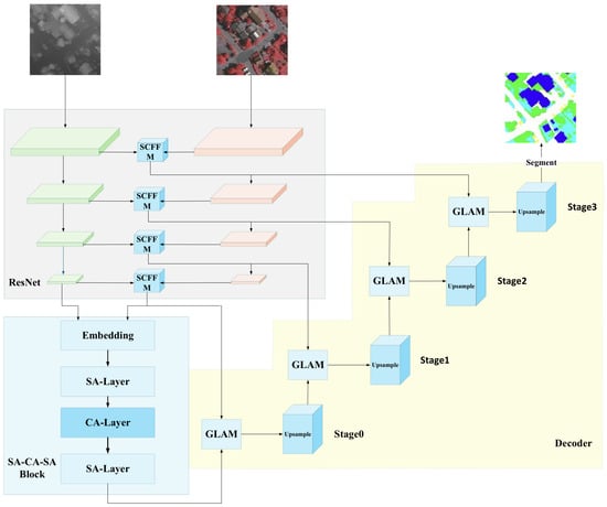
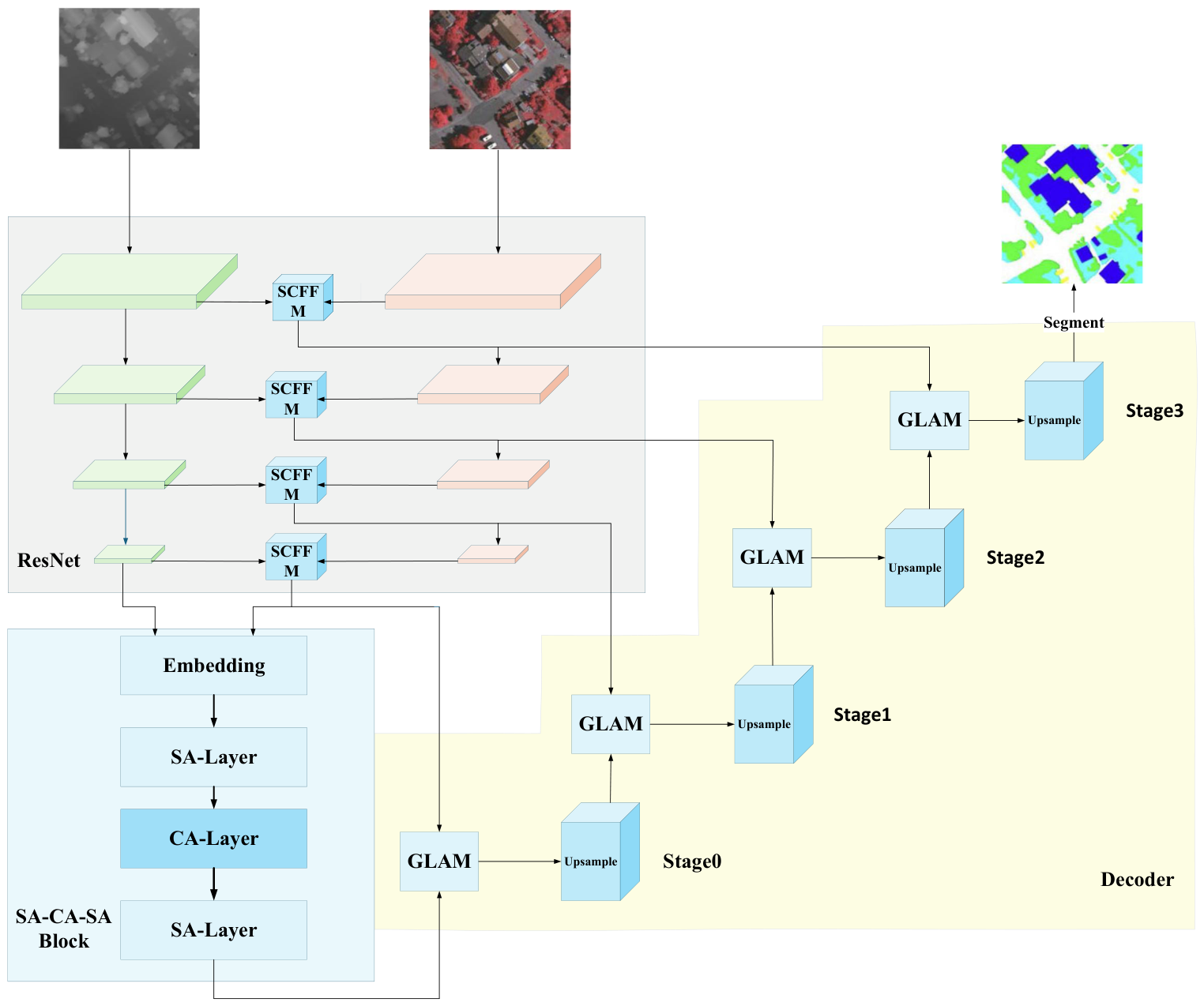
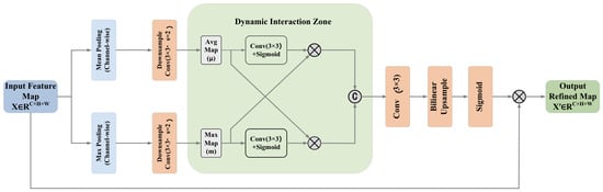
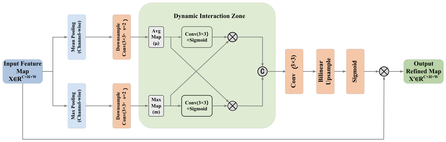


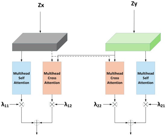
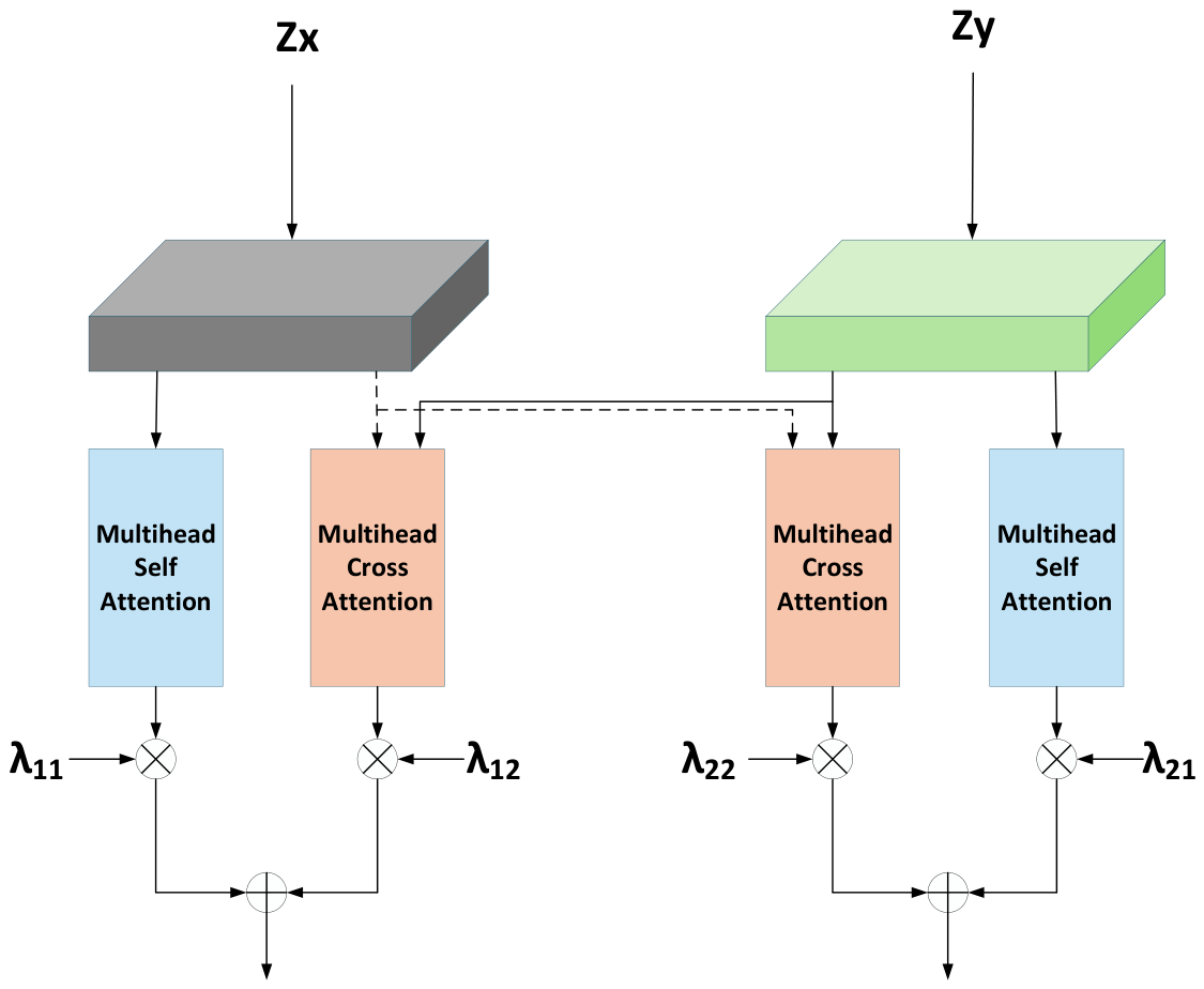
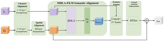
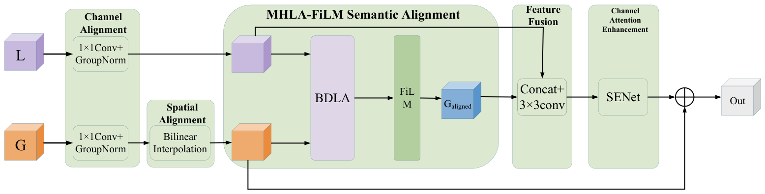
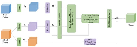
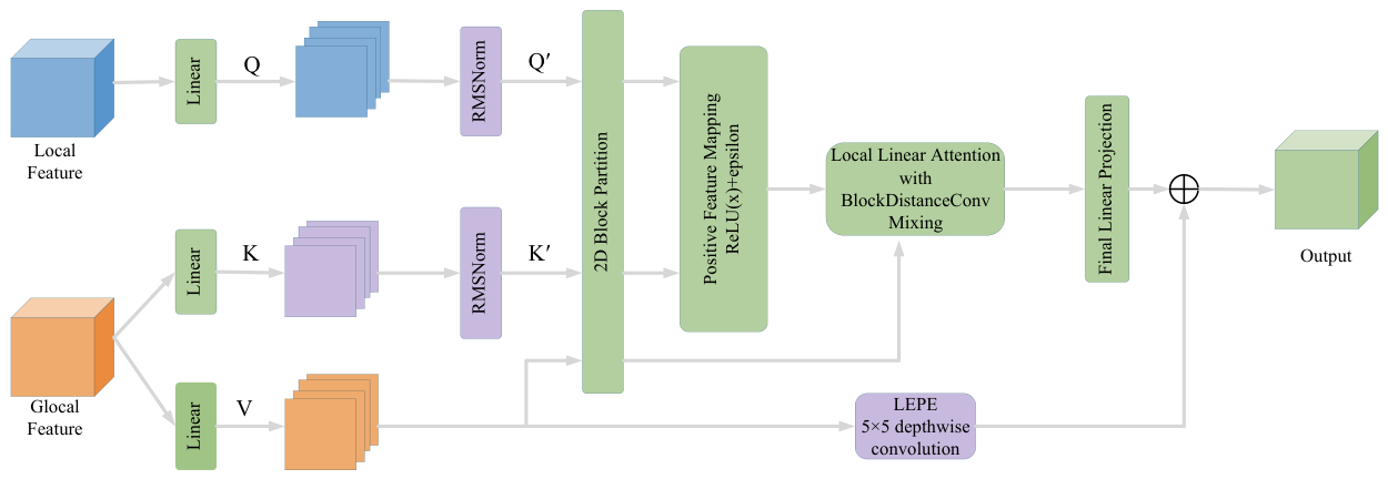
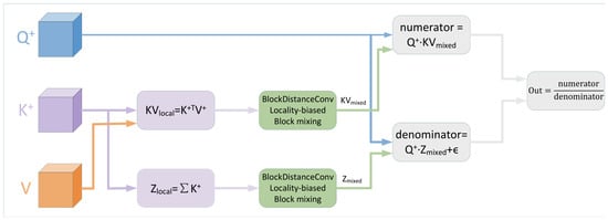
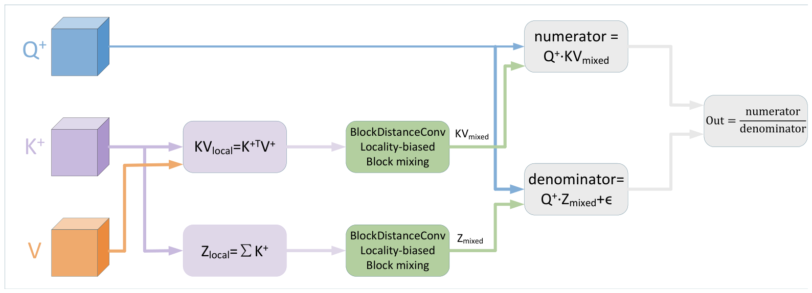
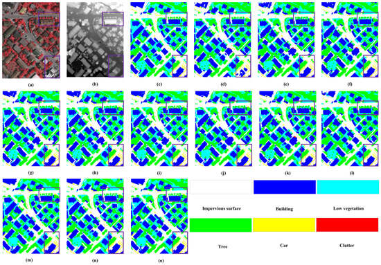
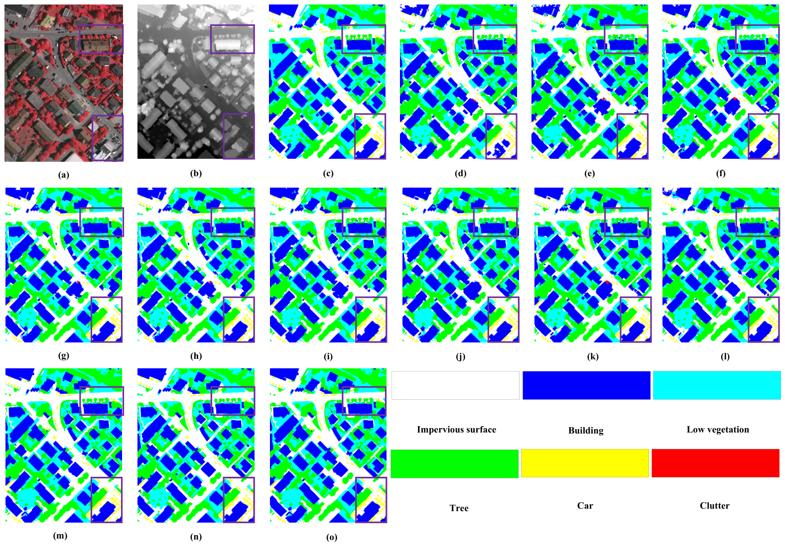
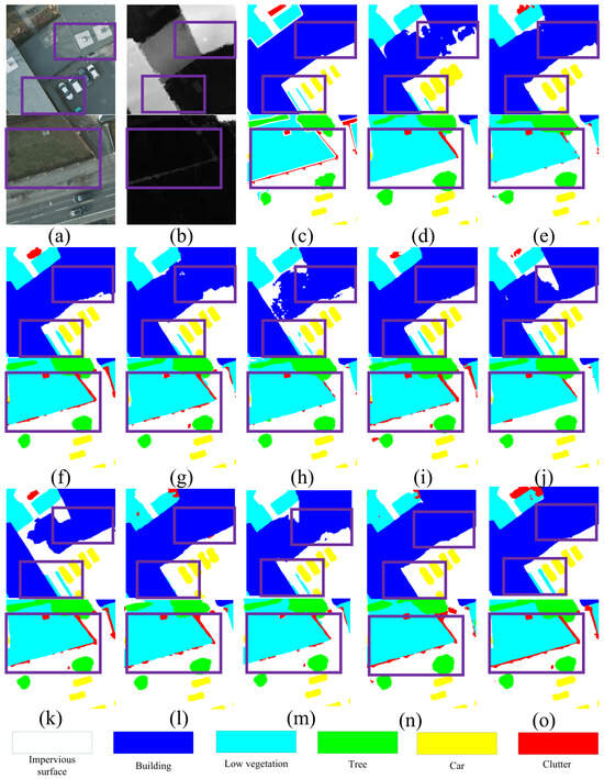
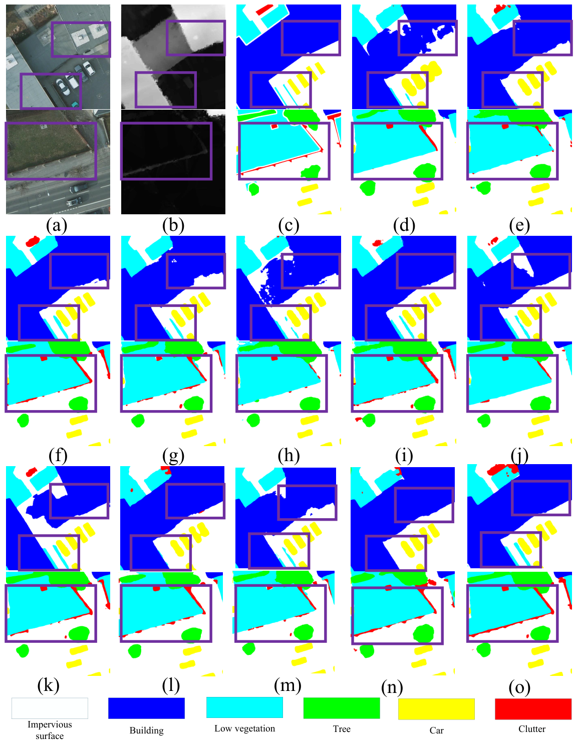
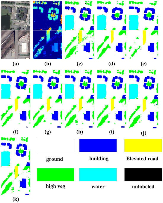
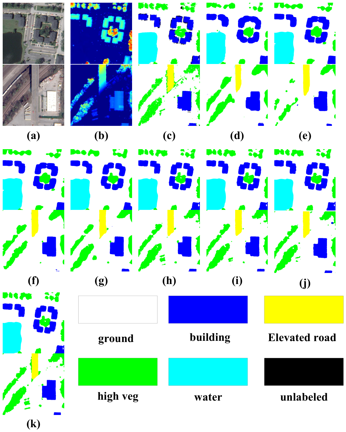
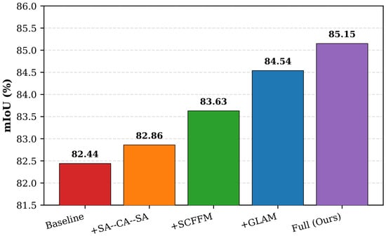
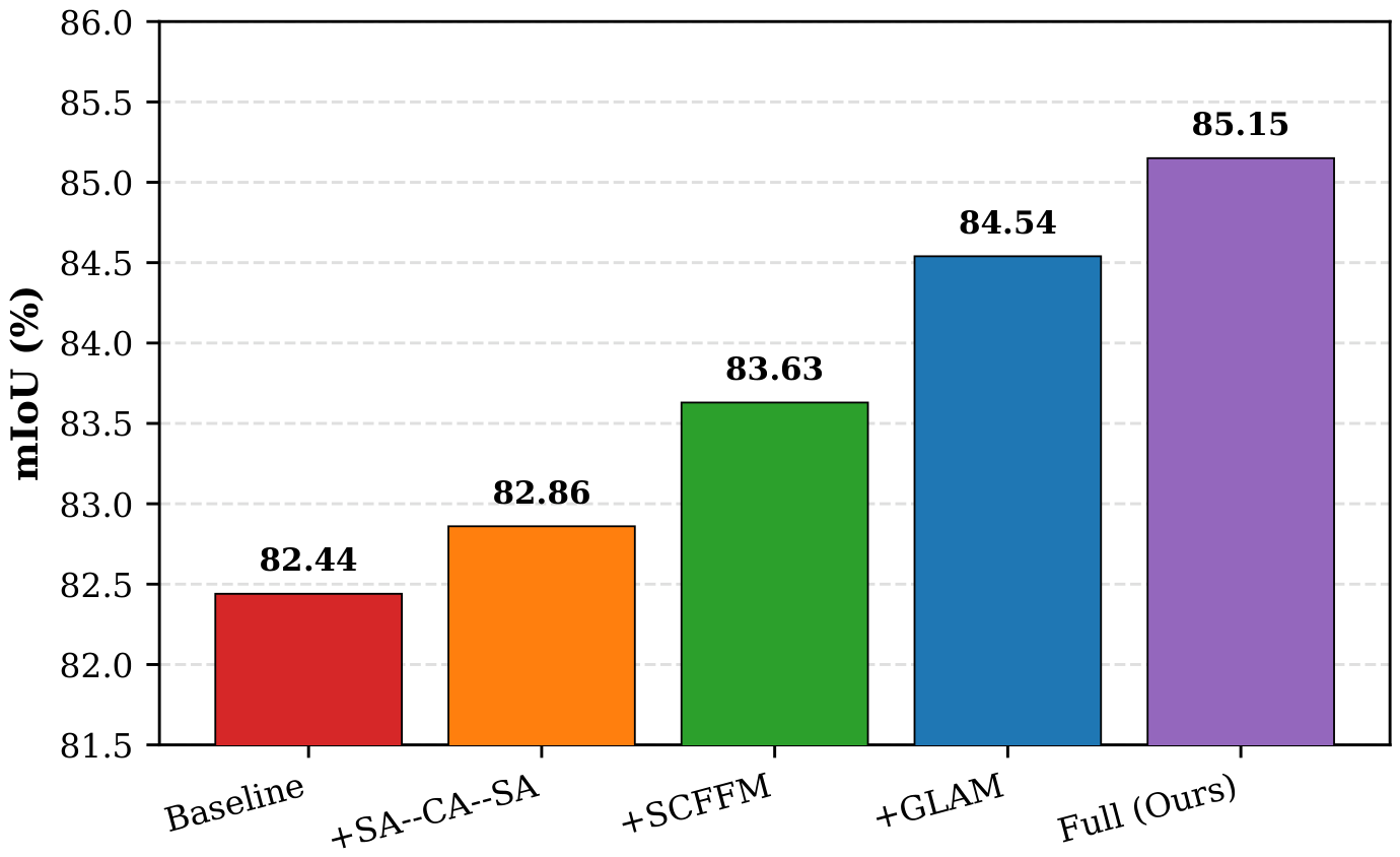
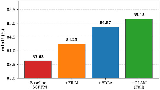
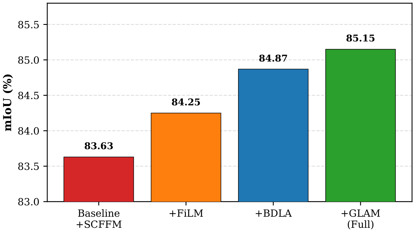
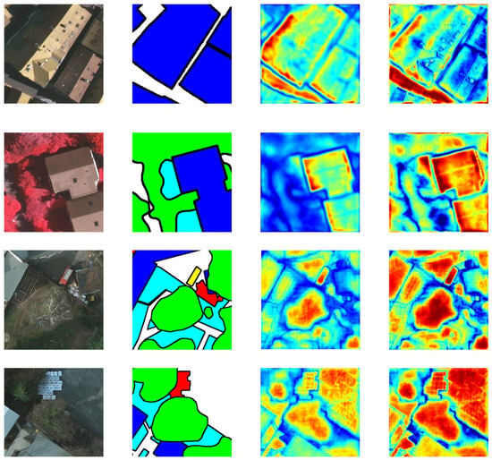
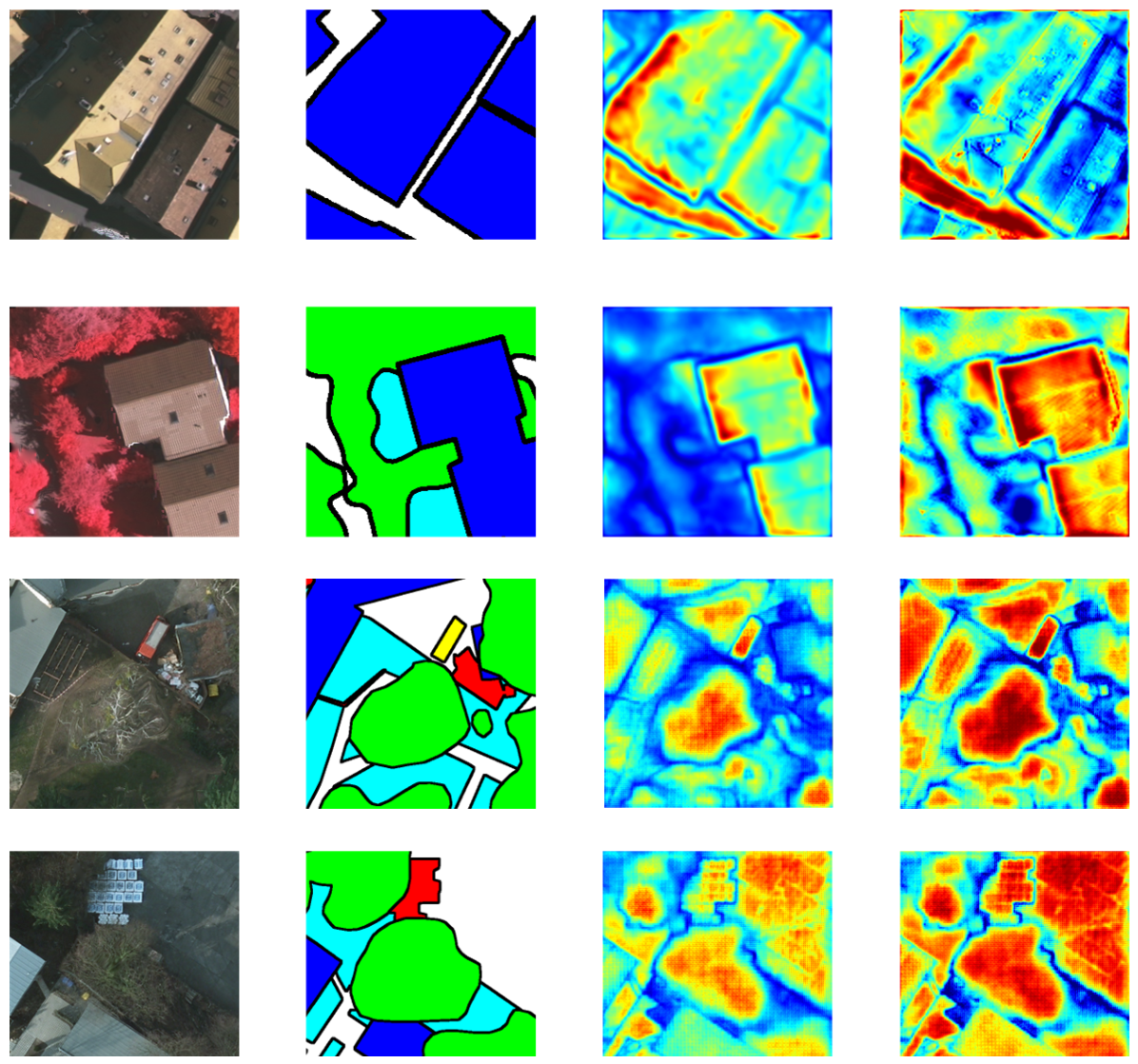

Disclaimer/Publisher’s Note: The statements, opinions and data contained in all publications are solely those of the individual author(s) and contributor(s) and not of MDPI and/or the editor(s). MDPI and/or the editor(s) disclaim responsibility for any injury to people or property resulting from any ideas, methods, instructions or products referred to in the content. |
© 2026 by the authors. Licensee MDPI, Basel, Switzerland. This article is an open access article distributed under the terms and conditions of the Creative Commons Attribution (CC BY) license.