


Highlights
What are the main findings?
- This paper proposes a decoupled differential search-based graph change detection network (DDS-Net), featuring a dual-stream encoder that automatically optimizes modality-specific feature extraction operators.
- A heterogeneous spatiotemporal alignment module (HSTAM) driven by a differentiable local search is designed to dynamically correct geometric misalignments and registration errors in the feature space.
What are the implications of the main findings?
- The decoupled differentiable Neural Architecture Search (NAS) strategy offers a novel, adaptive paradigm for heterogeneous change detection, overcoming the limitations of predefined and fixed network architectures.
- The model demonstrates strong generalizability and superior robustness in complex tasks, effectively handling severe spatial misalignments while maintaining high computational efficiency.
Abstract
With the advancement of Earth observation technology and the improvement of multisource data acquisition capabilities, heterogeneous remote sensing image change detection technology has become increasingly important. However, existing heterogeneous remote sensing image change detection methods rely largely on fixed network architectures, which makes adapting to complex modal differences and severe noise interference difficult. To address these issues, in this paper, a decoupled differential search-based graph change detection network (DDS-Net) is proposed. First, the model designs a decoupled differential search-based dual-stream graph encoder (DDSGE). By decoupling the search space from the optimization strategy, it automatically optimizes feature extraction operators and graph topologies for different modalities, thereby significantly increasing feature adaptability while reducing computational complexity. Second, to address nonlinear geometric distortions between heterogeneous images, in this paper, a heterogeneous spatiotemporal alignment module that is based on differential localization search (HSTAM) is proposed. This module uses a local soft attention mechanism to dynamically correct registration errors in the feature space. Furthermore, to suppress erroneous graph connections caused by noise, structural consistency and smooth denoising (SCSD) loss is introduced, and deep semantic feedback and graph smoothing regularization constraints are collaboratively used to dynamically generate graphs, thereby effectively increasing the internal consistency of the transformed graph and suppressing misconnection noise. Extensive experimental results demonstrate that this method significantly improves the robustness and accuracy of the model in complex registration error scenarios while maintaining computational efficiency.
1. Introduction
With the rapid development of remote sensing technology, methods for acquiring Earth observation data have become increasingly diverse, which has resulted in data characterized by massive volume, multiple sources, and heterogeneity. Traditional remote sensing image change detection methods rely largely on homogeneous imagery, thus requiring that dual-temporal images be acquired by sensors of the same type (e.g., both optical or both SAR) under similar imaging conditions. However, in practical applications, owing to constraints such as satellite revisit periods, meteorological conditions, and sudden disasters, obtaining high-quality homogeneous image data immediately is often difficult. In such cases, heterogeneous remote sensing image change detection (Hete-CD) becomes a key approach for addressing data gaps and improving temporal resolution.
Hete-CD involves effectively integrating data from different sensors to precisely analyze changes in multidimensional geographic information, thereby meeting the diverse demands of modern remote sensing technology in complex application scenarios. For example, in natural disaster assessment, synthetic aperture radar (SAR) imagery enables real-time monitoring of affected areas regardless of weather conditions, whereas optical imagery provides high-precision descriptions of post-disaster surface details. In the military and security sectors, Hete-CD is widely used to monitor activity changes in sensitive areas and urban transformations during armed conflicts [1]. In agricultural and forest resource management, by combining optical and hyperspectral imagery, changes in dynamic vegetation cover and crop growth conditions can be effectively detected. In emergency situations triggered by natural disasters, when homogeneous imagery is difficult to obtain, the use of Hete-CD to monitor land cover changes becomes particularly critical [2]. By leveraging the complementary strengths of different data sources, Hete-CD enables more comprehensive and precise monitoring of land surface changes. It not only provides robust support for emergency response, natural resource management, and the detection and rapid response to sudden incidents but also lays the foundation for long-term land surface condition monitoring.
Compared with homogeneous change detection (Homo-CD), Hete-CD faces greater challenges. Owing to the fundamentally different imaging mechanisms of various sensors, there are significant nonlinear differences in the radiative properties and statistical distributions of land features across different modal images [3,4], thus rendering direct pixel-level comparisons ineffective. Therefore, designing robust algorithms for bridging modal differences and effectively aligning and fusing heterogeneous features is a core scientific problem that urgently needs to be addressed in current heterogeneous change detection research.
In recent years, significant progress has been made in the field of Hete-CD. With their powerful topological modeling capabilities [5], graph neural networks (GNNs) have provided a new paradigm for addressing structural consistency issues in heterogeneous change detection. Unlike CNNs, which focus on local pixel neighborhoods, GNNs transform images into graph structures, which enables them to effectively capture long-range dependencies and global geometric features in non-Euclidean spaces—a capability crucial for identifying structural changes in objects across modal differences. However, in the application of GNNs to heterogeneous change detection, significant challenges are still faced: On the one hand, traditional graph construction methods typically involve high computational complexity, which makes meeting the processing demands of large-scale remote sensing imagery difficult; on the other hand, the significant differences in the spatiotemporal distributions of heterogeneous images make effectively aligning and interacting with heterogeneous features within a unified graph topology difficult. Therefore, designing an efficient graph structure construction mechanism that achieves precise spatiotemporal alignment of heterogeneous features while reducing computational costs has become a key challenge in further unlocking the potential of GNNs in this field.
To further explore the topological representation potential of graph neural networks in heterogeneous remote sensing image change detection (Hete-CD), overcome the limitations of traditional fixed graph architectures in adapting to multimodal physical differences, and address the inherent noise interference issues in heterogeneous data, in this paper, a decoupled differential search-based graph change detection network (DDS-Net) is proposed. The main contributions of this study are as follows:
- We propose a dual-stream graph encoder that is based on a decoupled differential search strategy. By constructing a modality-specific search space through a decoupled optimization mechanism, the model is freed from the constraints of a fixed architecture and can automatically select the optimal feature extraction operators for SAR and optical data, which significantly improves the adaptability of the model to heterogeneous features.
- To address the issue of spatiotemporal geometric inconsistencies in heterogeneous data, in this paper, a heterogeneous spatiotemporal alignment module is proposed. This module uses a differentiable local search strategy to achieve soft registration at the feature level, thereby effectively reducing false edge detection caused by registration errors and improving the spatial accuracy of change detection.
- To address the issues of severe noise interference and semantic bias in graph structures, in this paper, a structural consistency and smooth denoising loss is proposed. This loss function constrains the generation of graph structures in both the physical denoising and semantic consistency dimensions, thereby significantly improving the ability of the model to construct robust topological structures and suppress false changes.
The remainder of this paper is organized as follows. In Section 2, related work is reviewed. In Section 3, the overall architecture and core components of DDS-Net are presented in detail. In Section 4, the experimental results are presented and analyzed. Finally, in Section 5, the conclusions of this study are discussed.
2. Related Works
2.1. Heterogeneous Image Change Detection
From the perspective of learning frameworks, heterogeneous change detection (Hete-CD) techniques can be broadly classified into traditional algorithms and deep learning-based approaches. Within the traditional paradigm, parametric models rely primarily on multivariate or Gaussian mixture distributions to capture correlations between diverse sensor data and derive change measurements through parameter estimation. Prominent examples include the Kullback–Leibler distance metric, which was formulated by Mercier et al. [6]; the local copula model, which was established by Prendes et al.; and the M3CD Markov model, which was constructed by Touati et al. [3]. Similarity-driven techniques, such as the similarity map estimation introduced by Alberga et al. [7] and the patch similarity graph strategy developed by Sun et al., which leverages prior sparsity constraints and self-representation feature learning, focus instead on cross-modality pixel correspondences. Classification-oriented frameworks derive variations by contrasting the segmented maps of disparate remote sensing inputs, as demonstrated by the MS-CC technique, which was developed by Zhou et al., and the post-classification comparison (PC-CC) technique, which was used by Mubea and Menz [8] and Wan et al. Furthermore, transformation and projection methodologies aim to map heterogeneous data into a unified feature space. For instance, Luppino et al. applied image regression guided by pseudotraining data from a prior affinity matrix to translate source domains to target modalities, whereas Mignotte [9] used contraction mapping alongside adapted geometric fractal decomposition. In the realm of deep learning, convolutional neural networks (CNNs) dominate Hete-CD applications because of their robust ability to extract spatial attributes and recognize local patterns. These networks conventionally adopt multibranch topologies and process distinct modalities via separate feature extractors prior to conducting feature-space variation analysis. To mitigate inherent feature discrepancies across heterogeneous sources, various specialized networks have been developed, such as DA-MSCDNet, which was established by Zhang et al. [10] for domain adaptation; the transfer learning-driven MLSSN, which was developed by Jiang et al.; and the SCCN architecture, which was constructed by Liu et al. [11].
2.2. GNN-Based Heterogeneous Change Detection Algorithms
As a non-Euclidean data structure, a graph is composed primarily of nodes and edges, which can intuitively and effectively represent entities and their complex intrinsic relationships, respectively. To process such topological graph-structured data, graph neural networks (GNNs) are widely used as emerging deep learning architectures. The core of a GNN lies in efficiently modeling node relationships through information aggregation from local neighborhoods. In Section 3 of this paper, the standard GNN architecture proposed in [5] for feature extraction and processing is adopted.
To address the challenge of inconsistent feature representations in heterogeneous remote sensing images, GNN-based methods have made significant progress by modeling topological structures. Wu et al. [12] proposed a multiscale graph convolutional network that combines object-oriented analysis techniques with GCNs and treats segmented objects as graph nodes to aggregate multiscale contextual information, thereby effectively improving the robustness to noise in both homogeneous and heterogeneous image change detection. Building on this, to increase the discriminative power of features, Lv et al. [13] proposed a graph contrastive learning network (GCLN). This network constructs superpixel-based paired graphs, uses a graph feature learning module to capture near- and far-range dependencies among nodes and designs a contrastive loss function to maximize the difference between similar and dissimilar features, thereby widening the distance between unchanged and changed regions in the feature space. To address the challenge of predefined, fixed graph structures struggling to adapt to complex scenes, Xiao et al. [14] proposed a change-alignment-based graph structure learning method (CAGSL). This method involves using a graph autoencoder to dynamically optimize the graph topology and innovatively imposing change-alignment constraints. By leveraging the consistency of structural differences between the forward and backward directions to guide graph structure generation, it achieves high-precision detection in an unsupervised setting. Recently, Sun et al. further highlighted the limitations of traditional unsigned graphs in representing structural information and proposed a symbol-graph-based image transformation method (SGIT). In this method, a symbol-graph model is constructed by introducing positive and negative weights to represent similarity and dissimilarity relationships, respectively, and adaptive weighting is combined with neighborhood expansion strategies to transform heterogeneous images into structurally consistent intermediate representations, thereby effectively overcoming the challenges posed by differences in imaging mechanisms across heterogeneous sensors.
2.3. Neural Architecture Search
Neural architecture search (NAS) aims to automatically determine the optimal neural network architecture for a specific task through algorithms, thereby replacing the time-consuming manual design process [15,16]. To address the computational bottleneck of early discrete search methods, differential architecture search (DARTS) [17] was proposed. By using continuous relaxation, DARTS transforms architecture selection into a continuous variable learning problem that can be optimized via gradient descent, which significantly reduces end-to-end search costs and has become the current mainstream paradigm.
In the field of automated GNN design, NAS has effectively addressed the challenge of designing complex graph topologies and operator combinations. The SANE framework, which was proposed by Zhao et al., enables the automated construction of specific GNN architectures. Subsequently, GASSO [18] integrates structure learning into the search framework, which improves the robustness of the model to low-quality data contaminated by noise. To address the optimization bias caused by parameter coupling in traditional differentiable search, Chen et al. [19] proposed D2GNAS, which uses a decoupled differential search strategy and significantly improves the accuracy of architecture evaluation. When handling heterogeneous graphs, DiffMG [20] uses differentiable strategies to automatically search for subgraphs, thereby enabling efficient modeling of complex interactions.
In the field of remote sensing image change detection, NAS has been preliminarily applied to overcome the performance bottlenecks of fixed architectures. For example, Shi et al. used evolutionary algorithms to search for SAR change detection network structures, Gong et al. [21] specifically searched for GAN architectures for SAR change detection, and Zhang et al. [22] proposed a multiscale transformer architecture search method. However, the results obtained in previous work are primarily concentrated in the homogeneous change detection scenario. Applying the automated design capabilities of NAS to the field of Hete-CD, where nonlinear distortions and modal differences are more pronounced, remains a research direction that urgently awaits exploration.
3. Methodology
3.1. Overall Structure
As shown in Figure 1, the overall architecture of this method consists primarily of three core components: heterogeneous image construction and dual-stream decoupled search encoding, heterogeneous spatiotemporal alignment and feature reconstruction, and dynamic optimization on the basis of structural consistency and smooth denoising.
Figure 1.
The architecture of the proposed approach DDS-Net.
During the data input and graph construction stage, the network receives dual-phase heterogeneous images (e.g., SAR images at time T1 and optical images at time T2). To reduce the computational complexity and preserve the ground-truth boundary information, the raw images are first preprocessed using the super-pixel local information clustering (SLIC) algorithm, which aggregates pixels with similar spectral characteristics into super-pixel nodes and constructs an initial graph structure on the basis of adjacency relationships. These super-pixel nodes are then fed into the two branches of the dual-stream network.
In the feature encoding and alignment stage, unlike traditional methods that use weight-sharing twin networks, a dual-stream decoupled differential search encoder is used, as described in this paper. The SAR branch and the optical branch have independent architectural search spaces. Through a decoupled optimization strategy, the network can automatically search for feature extraction operators best suited to the physical characteristics of each modality from a library of candidate operators (including GCN, GAT, and GraphSAGE). After deep node features are extracted, a heterogeneous spatiotemporal alignment module is used to address geometric misalignment issues. This module uses a differentiable local localization search mechanism to dynamically identify features within the local neighborhood of T2 images that best match the semantics of T1 nodes and uses soft attention weights for feature reregistration to eliminate the effects of registration errors.
During the difference analysis and optimization stage, the aligned dual-phase features are mapped to the same latent space for contrastive learning, thereby generating the final change difference map. To ensure the reliability of the graph structure, the training process is supervised by a loss function that combines structural consistency and smooth denoising. This loss function uses deep semantic feedback to correct erroneous graph connections in shallow layers (cross-layer consistency) and a graph Laplacian regularization term to suppress false edges caused by SAR speckle noise (smooth denoising). The entire network is trained end-to-end and ultimately yields high-precision binary change detection results.
3.2. Dual-Stream Decoupled Search Graph Encoder (DDSGE)
In the change detection task for heterogeneous remote sensing images, SAR and optical images exhibit fundamental differences in terms of imaging mechanism, noise distribution, and feature characteristics. Traditional twin-network architectures force the use of feature extractors with shared weights, thus ignoring this intermodal heterogeneity, which makes achieving optimal feature representations across both modalities simultaneously difficult for the network. To address this issue, in this section, a dual-stream decoupled search graph encoder (DDSGE) is proposed, with the aim of using neural architecture search (NAS) technology to overcome symmetry constraints and automatically evolve the most suitable graph neural network topologies for the SAR and optical image branches.
In previous studies, the construction of graph structures relied primarily on K-nearest neighbor (KNN) algorithms that are based on color or spatial distance. This predefined, static graph construction method faces significant challenges when heterogeneous remote sensing images are processed: On the one hand, the speckle noise inherent in SAR images causes distance metrics in the feature space to fail, thereby introducing many erroneous connections (i.e., noise edges) into the graph structure that forcibly link otherwise unrelated ground object nodes; on the other hand, static graph structures remain unchanged throughout the entire network training process, and topological relationships cannot be automatically adjusted on the basis of task feedback, which causes graph neural networks to suffer from excessive smoothing and blurring of the boundaries between changing and invariant regions.
To address these issues, we first designed a differentiable structure generator. This generator dynamically predicts the probability of edges existing between nodes on the basis of their current semantic features, thereby reweighting and correcting the initial noisy graph. Specifically, for any two nodes and in layer , we calculate their feature similarity and combine it with learnable structural parameters to generate a dynamic adjacency matrix . The calculation formula is as follows:
where represents the learned connection weight between nodes and ; maps the weight to the interval via the sigmoid activation function; represents the initial static adjacency matrix (including noise) constructed using KNN; represents a lightweight edge prediction network whose input is the concatenation of node features represents a hyperparameter that balances the initial structure and the learned structure.
Second, we constructed a dual-stream hypernetwork that contains a rich variety of operation types, as illustrated in Figure 2. In each layer of the hypernetwork, the output features of node are no longer generated by a single convolutional operation but are defined as a weighted mixture of the outputs from all the operations in the candidate operator set . This mixed operation mechanism enables the network to explore possible combinations of different operators within a continuous search space. It formalized as follows:
where denotes the output feature vector of node in layer , denotes the set of candidate operators, represents the selection mask (Mask) that corresponds to the th operator in layer , represents the specific graph convolution operation function, represents the learnable weight parameter that corresponds to this operator, and denotes the set of neighboring nodes of node .
Figure 2.
Architecture of the DDSGE.
To construct a search space that can cover a wide range of graph topological characteristics and have strong expressive power, we define a set of candidate operators to include representative graph convolution and auxiliary operations.
(1) Graph convolutional networks (GCNs) use a first-order approximation of spectral graph theory to smooth local features and are suitable for extracting low-frequency global information. Their feature update formula is defined as follows:
where denotes a nonlinear activation function (e.g., ReLU), represents a normalization constant that is based on the node degree and is used to prevent feature value explosion, and represents the linear transformation matrix of the current layer.
(2) Graph attention network (GAT): To address the issue of inconsistent importance among nodes in different neighborhoods within heterogeneous images, the GAT dynamically computes aggregation weights via a self-attention mechanism. The calculation formula is as follows:
where represents the attention weight of node for node , is a learnable attention vector, and denotes the vector concatenation operation.
(3) GraphSAGE uses an inductive neighbor aggregation strategy in which max or mean pooling is applied to increase the robustness against high-noise data (such as SAR speckle noise). Its update rule is formulated as follows:
where AGG(•) denotes an aggregation function (e.g., mean or max pooling) used to integrate neighborhood feature information.
(4) Graph isomorphism network (GIN): The GIN improves the ability to distinguish graph isomorphism structures. Its formula is as follows:
where represents a learnable scalar parameter used to adjust the weight of the features of the central node and MLP denotes a multilayer perceptron.
The set also includes the identity mapping (Identity) for constructing residual connections, as well as the zero operation (Zero) to enable the network to disconnect unnecessary connections, thereby enabling the network to automatically adjust its depth.
After the search space is defined, traditional differential NAS methods (such as DARTS) typically face a severe coupled optimization bias problem, where the architectural parameters and the network weights are updated in a coupled manner within the same computational graph, which leads to the search process easily overfitting simple operators in the early stages of training. To address this core issue, in this section, a decoupled sampling mechanism that is based on Gumbel–softmax is introduced. Instead of directly using the softmax-normalized for weighting, we introduce a noise vector that follows a Gumbel (0, 1) distribution. By applying the continuous relaxation form of the Gumbel–Max technique, the generated soft-sampled weights are computed as follows:
where represents the architectural parameter of the ith operator; represents the noise sampled from the Gumbel distribution, with represents the temperature coefficient, which gradually decreases to 0 as training progresses.
To ensure the discreteness of the architecture during forward propagation and to conserve video memory, we use argmax to generate a hard mask that participates in the actual computation, but during backpropagation, we use a straight-through estimator (STE) to approximate the gradients, as expressed in the following formula:
In particular, is a discrete vector obtained by one-hot encoding on the basis of , and the stop_gradient () operator blocks gradients from flowing through the terms inside the brackets during backpropagation, thereby achieving discretization of forward computation and differentiability of backpropagation.
On the basis of the above sampling mechanism, in this section, a gradient truncation strategy and a two-layer optimization algorithm are proposed to completely eliminate the dependence of weight updates on architectural parameters. We model the search process as an alternating two-layer optimization problem. In the inner optimization stage, we fix the distribution of architectural parameters on the training set, sample discrete architectural paths, and update only the hypernetwork weights . Most importantly, in this step, we implement a gradient truncation strategy in which we forcibly cutting off the gradient flow from the task loss back to the architectural parameters . Hence, the update formula for the weights is as follows:
where represents the learning rate for the weights, represents the training dataset, and the constraint explicitly indicates that when the weight gradients are computed, the architecture sampling results are treated as constants, and the gradients are not propagated back to via the chain rule. In the outer loop phase, we fix the weights that have already undergone decoupled training, evaluate the performance of the current architecture distribution on the validation set, and update the architectural parameters :
where represents the learning rate for the architectural parameters and represents the loss function on the validation set. At this point, because the weights have already been thoroughly and independently trained in the inner loop, the gradients from the validation set can truly reflect the merits of the architecture rather than providing a false impression of weight fitting. Through this alternating decoupling optimization strategy, the search process avoids architectural collapse. Ultimately, by selecting the operator that corresponds to the maximum value of the architectural parameters, it derives definite heterogeneous network structures for the SAR and optical branches, thereby fundamentally resolving the issues of feature misalignment and modal imbalance in heterogeneous data.
3.3. Heterogeneous Spatiotemporal Alignment Module (HSTAM)
Existing graph neural network-based methods for detecting changes in heterogeneous images are typically based on the assumption of static pixel- or superpixel-level alignment, i.e., that the position (x, y) in the image at time strictly corresponds to the same position in the image at time . However, in practical applications, owing to differences in sensor imaging angles, geometric distortions caused by terrain undulations, and residual errors during image registration, this ideal pixel-level correspondence is often difficult to achieve. Inspired by the dynamic heterogeneous attention mechanism in DHGAS [23], in this section, a heterogeneous spatiotemporal alignment module (HSTAM), which is embedded between the feature extractor and the comparison loss function, is proposed. Drawing on the location-space search concept from DHGAS, this module does not assume fixed node connections but instead adaptively learns a cross-temporal alignment matrix through differentiable neural architecture search to achieve feature alignment.
An architectural diagram of the HSTAM is shown in Figure 3. Its core lies in the construction of a searchable localization space, which enables the network to automatically find the optimal feature matching paradigm. We define the search domain at time for node i at time as the set of spatial positions of its K-jump neighbors. To accommodate the complex nonlinear feature relationships in heterogeneous images, we no longer use a single fixed similarity function (such as the dot product) but instead construct a library of candidate operations that includes various matching operators (such as bilinear matching, cosine similarity, Gaussian kernel distance, and neural network projection). Element in the localization matrix represents the matching probability between node at and node at . This probability is obtained through a weighted ensemble search of the candidate operators. The calculation formula is as follows:
where represents the cross-temporal attention weights, denotes the set of candidate matching operators, represents the architectural search parameters for the th matching operator (discretized by Gumbel–softmax sampling), and represent the node feature vectors extracted by the dual-stream heterogeneous feature encoder proposed in Section 3.2, and denotes the spatial neighborhood set of node in the cross-temporal graph.
Figure 3.
Architecture of the HSTAM.
On the basis of the estimated localization matrix , the HSTAM performs feature reconstruction to generate the spatiotemporally aligned features at time . The physical interpretation of this step is as follows: for each node in , we do not directly compare it with the node at the corresponding coordinate in ; instead, we use the learned localization weights to aggregate a virtual feature vector within the local neighborhood of that is most similar to . If and have merely undergone geometric displacement because of registration errors, the localization mechanism can capture the correct corresponding features, thereby ensuring that the aggregated feature is highly similar to and eliminating false positives; conversely, if a genuine change in the ground truth has occurred, no matching features will be found within the neighborhood, thus resulting in a significant discrepancy between the aggregated result and the original feature. The feature reconstruction formula is defined as follows:
where represents the aligned feature vector that corresponds to node at time , which is obtained by the weighted summation of features from all potential corresponding nodes within the neighborhood at time .
Finally, to address the issue of false positive arising from the direct comparison of unaligned features in traditional methods, we designed a robust difference metric that is based on aligned features. This mechanism enables the model to focus on capturing essential semantic changes rather than physical misalignments at the geometric level. Specifically, we feed the original features at time step T1 and the aligned features at time step T2—generated by the HSTAM—into a difference discriminator network (composed of a multilayer perceptron, MLP), thereby computing the final change intensity map. The calculation formula is as follows:
where represents the change probability score for node i; and are the learnable weights and biases, respectively, of the difference discriminator; and denotes the sigmoid activation function. By introducing the HSTAM, we unify the registration and discrimination subtasks in change detection into a single end-to-end differential search framework, thereby significantly improving the robustness and accuracy of the algorithm described in this section on heterogeneous, misaligned datasets.
3.4. Structural Consistency and Smooth Denoising Loss (SCSD Loss)
To address the issue of unreliable initial graph structure connections caused by inherent speckle noise in heterogeneous remote sensing images, as well as the lack of task-aware feedback mechanisms in existing graph construction methods, in this section, structural consistency and smooth denoising loss (SCSD loss) is proposed. The aim of this strategy is to establish a closed-loop feedback mechanism that spans both shallow and deep layers of the network, thereby enabling the coevolution of graph topology and feature representations. To establish a feedback channel from deep features to shallow structures, we first design a cross-layer structural consistency loss, . By minimizing the discrepancy between the dynamic adjacency matrix and the deep semantic similarity matrix, this loss forces the dynamic adjacency matrix generated by the front end to predict the similarity distribution of deep features output by the back-end encoder. By using high-order semantic information to retroactively supervise the topological generation process in the shallow layers, this loss function is defined as follows:
where denotes the time step that corresponds to (SAR image) and (optical image); represents the dynamic adjacency matrix predicted by the front-end dynamic graph generator for time step , in which represents the number of superpixel nodes; represents the deep high-order semantic feature matrix output by the dual-stream decoupled encoder (DSDE), in which denotes the feature dimension; and represents the autocorrelation similarity calculation function, for which normalized cosine similarity is adopted, i.e., , to measure the semantic association between nodes in the deep feature space, where denotes the Frobenius norm, which is used to calculate the elementwise mean squared error between two matrices.
Furthermore, to filter out heterogeneous spot noise and control the connectivity density of the graph, we introduce a graph smoothing denoising regularization term that incorporates both Dirichlet energy and sparsity constraints. This regularization term is based on smoothness priors in graph signal processing and aims to physically sever high-frequency noise edges that connect dissimilar features. Its calculation formula is as follows:
where represents the connection weight between node and node in the dynamic adjacency matrix and and denote the initial input features (such as color, texture, or shallow embeddings) of nodes and , respectively, at time step . The first term in the formula is a smoothing term, where represents the difference between the two nodes in the original feature space. Minimizing this term forces the network to reduce the connection weights between nodes with significantly different original features (which typically correspond to noise or edges), thereby achieving denoising. The second term is the sparsity regularization term, where represents the sparsity regularization coefficient used to control the sparsity of the graph structure to prevent the generated graph from becoming overly dense and causing excessive smoothing during information propagation in the graph neural network.
To precisely detect changes in heterogeneous objects, for the main task loss , a robust contrastive loss function that is based on HSTAM-aligned features is used. This loss function aims to bring unchanged regions closer together in terms of feature distance while pushing changed regions farther apart. Given the true label of the th node (where denotes unchanged and denotes changed) and the feature distance , which is defined as follows:
where represents the total number of nodes and represents the edge threshold, which is used to ensure that the feature differences in the changed regions are sufficiently significant. To ensure an unsupervised framework that is fair for comparison with existing unsupervised methods, we operate DDS-Net without manual annotations. Instead of using the ground-truth label for , we generate pseudo-labels dynamically by applying Otsu’s thresholding method to the feature distance map obtained in the early stages of training. By substituting the ground-truth with the unsupervised pseudo-label , the contrastive loss guides the training process in an unsupervised manner. Finally, to jointly optimize the graph structure and feature representations during end-to-end training, we define the overall objective function as a weighted combination of the change detection main task loss, the cross-layer structural consistency loss, and the graph smoothing denoising regularization term, which is calculated as follows:
where and are balancing coefficients used to adjust the weights of the auxiliary structural constraints in the main task optimization. By minimizing this total objective function, the model can adaptively adjust the graph topology to accommodate the characteristics of heterogeneous data while optimizing the change detection performance.
4. Experiments
4.1. Experimental Introduction
4.1.1. Datasets
In our experiments, five heterogeneous remote sensing image datasets that cover different sensor types, scales, geographic regions, and change types were used. As shown in Figure 4, among these datasets, the Gloucester I [14] datasets, along with the Gloucester II [24] datasets, consist of combinations of optical and SAR imagery and are used to detect flood-affected areas in different time periods. The Shuguang dataset also includes cross-modal optical and SAR imagery, with a focus on changes in landforms such as construction sites and rivers. The Texas [25] dataset documents changes before and after forest fires and consists of multispectral optical images acquired from different platforms; its heterogeneity stems from nonoverlapping spectral bands. The Toulouse dataset consists of RGB images with distinct spectral band characteristics and is used to enable fine-grained monitoring of urban road construction progress.
Figure 4.
All the datasets used in the paper. (a) Gloucester I, (b) Gloucester II, (c) Texas, (d) Toulouse, and (e) Shuguang.
4.1.2. Implementation Details
The DDS-Net model was implemented using the PyTorch framework, the software environment was built on Python 3.8 and PyTorch 1.12.1. Both training and inference were performed on a workstation equipped with an NVIDIA GeForce RTX 3080 GPU. During the data preprocessing stage, the SLIC algorithm was used to perform superpixel segmentation on the input images. The number of superpixels was set to 2500 for the Gloucester I and Gloucester II datasets, 2000 for the Texas and Toulouse datasets, and 1000 for the Shuguang dataset. The model was trained using the Adam optimizer, with an initial learning rate of 1 × 10⁻³ and a weight decay coefficient of 5 × 10⁻⁴. The total training duration was 200 epochs, with the first 50 epochs serving as a warm-up phase (during which only network weights were updated), followed by alternating optimization of weights and architectural parameters. Additionally, the initial temperature for Gumbel–softmax sampling was set to 5.0 and gradually reduced to 0.1 using an exponential annealing strategy, and the weight coefficient for the structural denoising loss in the joint loss function was set to 0.1.
4.1.3. Evaluation Metrics
To quantitatively evaluate the classification performance and spatial consistency between the change maps predicted by the model and the ground-truth annotations, five metrics—precision, recall, F1 score, overall accuracy (OA), and kappa coefficient (KC)—were used for comprehensive assessment. Specifically, precision and recall were used to quantitatively assess the ability of the model to suppress false positives and reduce false negatives, respectively; the F1 score was used to evaluate the overall balance between precision and comprehensiveness of the model; and the overall accuracy was used to assess the overall classification accuracy of all pixels. The kappa coefficient, which measures classification accuracy by considering random agreement, is typically used to evaluate the reliability of remote sensing image classification. These metrics collectively provide a robust and multifaceted evaluation of the heterogeneous change detection performance.
4.2. Comparison Experiments
To validate the effectiveness and superiority of the proposed method, seven state-of-the-art methods were selected for comparison, as described in this section. These methods were chosen because they represent the current state of the art in their respective categories and their source code is open source. Among them, three methods, namely, refs. [26,27] sparse constrained adaptive structural consistency (SCASC), adaptive graph and structural cyclic consistency (AGSCC), and SR-GCAE [28], are based on graph theory; the other four methods, namely, X-NET [29], the adversarial cyclic encoder network (ACE-NET) [29], the code alignment autoencoder (CAE) [30], and SCCN [11], are image regression and feature transformation methods that are based on convolutional neural networks.
All of the above methods fall under the category of unsupervised methods and can be compared with the proposed method. The parameter settings for the selected methods are set to the default values reported in their respective papers to ensure fairness in the comparison.
4.2.1. Quantitative Analysis
To comprehensively evaluate the performance of the method proposed in this paper, we conducted a quantitative comparison with the seven advanced Hete-CD methods mentioned above across five public datasets. To ensure a fair comparison with these state-of-the-art unsupervised baselines, our proposed DDS-Net was evaluated in its unsupervised configuration (relying on pseudo-labels, as detailed in Section 3.4), without any access to ground-truth labels during training. As shown in Table 1, the method proposed in this paper demonstrated strong competitiveness in terms of core comprehensive metrics such as precision, F1 score, and kappa coefficient on most datasets, although some fluctuations in certain individual metrics occurred.
Table 1.
Quantitative comparison of the performance of the method described in this paper against that of the other methods on the five datasets (the best results are presented in bold).
Specifically, our method demonstrated outstanding overall recognition performance on the Gloucester I and Toulouse datasets. On the Gloucester I dataset, our method achieved an F1 score of 81.8% and a precision of 81.2%. Although the SCASC and AGSCC methods achieved high overall accuracy rates of 97.8% and 97.3%, respectively, their prediction strategies were overly conservative, and these high rates were achieved at the cost of significant numbers of false-negatives. In contrast, our method effectively balances precision and recall through the heterogeneous spatiotemporal alignment module, thereby achieving optimal overall performance while ensuring the complete extraction of changing objects. On the Toulouse dataset, which is particularly challenging for detection, our method similarly overcame the conservative prediction shortcomings of the comparison methods and achieved an F1 score of 54.1%, thus demonstrating a clear advantage over all the compared methods. The Shuguang dataset features complex building clusters that are highly prone to false positives and places greater demands on the comprehensive recognition capabilities of the model. Our method achieved the best F1 score (82.5%) and the best precision (87.5%) on this dataset. Although the recall of the CAE method reached 85.5%, which was higher than that of our method (78.0%), its precision (78.8%) was far below that of our method. This finding indicates that the high recall of the CAE method is based on excessive region expansion and many false positives. Our method effectively suppresses high-frequency noise and severs false edge connections, thus demonstrating stronger false-positive suppression capabilities and outperforming the other methods in terms of overall performance. On the Texas dataset, our method achieved the best precision (90.8%) and a kappa coefficient of 87.0%. Because this dataset consists of highly homogeneous multispectral optical images, the AGSCC method, by leveraging its cyclic consistency architecture, achieved an F1 score of 90.8%, thus outperforming our method (which achieved a score of 89.9%). The CAE method led with a recall rate of 91.3%, but it similarly disrupts object boundaries, which resulted in a decrease in precision. Our method strictly limits the disordered expansion of regions, thereby ensuring the overall reliability of the detection results while maintaining high precision. On the Gloucester II dataset, our method achieved a precision of 92.8% and a kappa coefficient of 89.0%, maintaining its leading advantage in precision. Because the imaging regions in this dataset have relatively consistent geometric structures, the symmetric network adopted by the SCCN method exhibits exceptional adaptability when heterogeneous data with minimal spatial misalignment are being processed, which resulted in slight advantages in terms of the recall and F1 score in this study. The complex dynamic optimization space designed by our method is targeted primarily at extreme misalignment scenarios; although it introduces slight optimization redundancy when faced with such simple registration scenarios, it still performs best in suppressing false positives.
To evaluate the computational efficiency and the true cost-effectiveness of the model, both the inference runtimes (in seconds) and the total training costs (in GPU hours) of the selected comparison methods and our DDS-Net under various numbers of superpixel nodes (Ns) are presented in Table 2.
Table 2.
Comparison of inference runtimes (seconds) and total training time (GPU hours) between the method proposed in this paper and other methods under various numbers of super-pixel nodes (the best results are presented in bold).
Under the default configuration (Ns = 2500), DDS-Net took an inference time of 5.4 s and 7.9 s on the Gloucester I and Gloucester II datasets, respectively, and outperformed both the computationally intensive SCCN (70.1 s and 80.5 s, respectively) and the relatively lightweight X-NET (7.4 s and 13.2 s, respectively) baseline methods. These results demonstrate that by using superpixel segmentation for front-end preprocessing, combined with a decoupled search mechanism, the graph structure can be effectively compressed, and redundant computations during feature alignment can be significantly reduced. However, the inference runtime of DDS-Net is highly sensitive to the number of superpixel nodes. When Ns was increased to 5000 and 10,000, the computational load for dynamic alignment and the search space surged nonlinearly because of the expansion of the graph node scale, which caused the inference runtime of the model to increase sharply. At Ns = 10,000, the inference runtimes reached 74.9 s and 83.5 s, respectively, and approached or even exceeded those of some traditional baseline models. On the basis of the above inference runtime data, the total number of superpixel segments for the Gloucester I and Gloucester II datasets was set to 2500 in the experiments. This configuration optimizes computational efficiency while ensuring fine-grained features, thereby guaranteeing the satisfactory inference runtime of the model in practical deployment. Furthermore, to evaluate the overall cost-effectiveness, the total training and search time for our DDS-Net (under the default configuration of Ns = 2500) required only 1.6 and 2.1 GPU hours on the Gloucester I and Gloucester II datasets, respectively. Although neural architecture search (NAS) inherently requires a higher upfront computational investment during the training phase, our method effectively mitigates this burden. By compressing the raw images into a compact super-pixel graph and utilizing an efficient two-level decoupled optimization strategy, the computational overhead is significantly reduced. As a result, the training time of DDS-Net is much lower than that of computationally intensive methods like SCCN (8.5 and 9.8 h) and is even superior to lightweight baseline methods like ACE-NET. This demonstrates that our approach not only yields a highly optimized and compact structure for practical inference deployment but also maintains exceptional training efficiency.
4.2.2. Qualitative Analysis
In Figure 5, the change detection results of the proposed DDS-Net and seven mainstream comparison algorithms across five heterogeneous datasets are visually illustrated. The visual results are highly consistent with the quantitative evaluation metrics, thus further validating the advantages of our method in suppressing noise and overcoming spatial misalignment.
Figure 5.
Qualitative comparison of change maps generated by various methods on five datasets. (a) SCCN, (b) ACE-NET, (c) X-NET, (d) SCASC, (e) AGSCC, (f) CAE, (g) SR-GCAE, (h) our method, and (i) the true change map. FP (red); FN (green).
The first two rows show the results for the Gloucester I and Gloucester II datasets, which feature primarily flood-submerged areas. In such scenarios, the shapes of the affected regions are irregular, and their boundaries are complex. The SCCN, ACE-NET, and X-NET methods generated many false red pixels in the background areas and exhibited severe green false-negative results and discontinuities in the main flood areas, thus indicating that traditional CNN-based image regression methods struggle to effectively handle the strong nonlinear radiometric differences between optical and SAR images. Although the SCASC and AGSCC methods suppressed noise to some extent, significant jaggedness persisted along the boundaries. In contrast, our method (h) demonstrated the best visual performance on both datasets and not only produced extremely clean backgrounds but also accurately delineated the complex boundaries of the flooded areas. In the third row, the results for the Texas wildfire dataset are presented. The SCCN, X-NET, and CAE methods generated dense clusters of green false-positive pixels within the fire areas, which caused the change map to lose the structural integrity of surface changes. Our method (h), through global constraints imposed by structural consistency and smoothing denoising loss, maximized the preservation of structural integrity, with a false-negative rate that was significantly lower than those of all the other comparison algorithms. In the fourth and fifth rows, the results for the Shuguang dataset, which contains complex buildings and waterways, and the Toulouse dataset, which features fine-grained road infrastructure, are presented. In such urban scenes with significant geometric distortion and nonlinear spatial misalignment, the performance of most of the baseline methods was severely degraded. For example, as shown in the fourth row, the SCCN, ACE-NET, and CAE methods generated extremely high rates of red false positives along building edges; as shown in the fifth row, SR-GCAE almost completely missed the slender road structures (shown as large areas of green). Our method (h) clearly captured subtle linear structures and building contours. These results fully demonstrate the effectiveness of the heterogeneous spatiotemporal alignment module (HSTAM) proposed in this paper for performing local soft alignment in the feature space, which enables the model to filter out geometric misalignment noise and focus on genuine semantic changes.
4.3. Ablation Experiments
4.3.1. DDSGE
To validate the effectiveness of the dual-stream decoupled differential search graph encoder (DDSGE) proposed in this paper and to investigate the specific contributions of neural architecture search (NAS) and the decoupling optimization mechanism to the performance of the model, six variant models with different configurations were designed for comparative experiments on the heterogeneous Texas and Toulouse datasets. These six variants are the standard baseline, which does not include the NAS module and uses a manually designed fixed graph convolutional network; the strong manual baseline, which utilizes a predefined mix of GCN, GAT, and GraphSAGE operators; the random baseline, which fully randomly samples operator combinations within the same search space; the shared-weight twin encoder baseline, which forces both branches to use identical searched architectures and shared weights; the DARTS coupled optimization baseline, which uses a traditional differential architecture search strategy with coupled updates of architectural parameters and weights; and the proposed method (Ours), which uses a two-layer decoupled optimization mechanism. The experimental results are shown in Table 3.
Table 3.
Ablation experiments for the DDSGE module (the best results are presented in bold).
Analysis of the experimental results reveals that the intelligent search strategy significantly outperforms both fixed designs and random combinations. The model that incorporates the differentiable search strategy achieved substantial improvements across all key metrics. Taking the Texas dataset as an example, the F1 score of the baseline model using a manually designed fixed strategy was only 70.1%. After random sampling within the same search space, the F1 score increased slightly to 75.9%, which indicates that the candidate operator space constructed in this study has high inherent potential value. However, the performance of the random strategy still lagged significantly behind the 90.7% achieved by our method. This comparison reveals that the heterogeneous change detection task is highly sensitive to graph operator combinations; random operator stacking fails to leverage the synergistic advantages of feature extraction, which fully validates the necessity of introducing intelligent architecture search to uncover optimal topological structures. Even when utilizing a strong manual baseline with a predefined mix of powerful operators (GCN, GAT, and GraphSAGE), the model achieved an F1 score of 82.5% on the Texas dataset. While this represents a significant improvement over the standard and random baselines, it still falls short of our method, confirming that relying solely on human priors is insufficient to handle complex topological variations. Additionally, to evaluate the necessity of modality-specific architectures, we tested a shared-weight twin encoder baseline. Although it employs our advanced decoupling optimization mechanism, it achieved an F1 score of 88.4% on the Texas dataset, experiencing a noticeable performance drop compared to our proposed method. This strongly validates our hypothesis: forcing heterogeneous modalities to share identical architectures and weights inherently limits the network’s ability to extract optimal modality-specific features. Furthermore, the decoupled optimization mechanism effectively overcomes the performance bottlenecks of traditional coupled optimization. While sharing the same search space, the introduction of the two-layer decoupled optimization mechanism further improved the evaluation metrics of the model on both heterogeneous datasets. On the Toulouse dataset, where changes are more subtle, the F1 score of the traditional DARTS coupled optimization strategy was 53.2%, whereas that of our method was 55.0%, with a corresponding increase in overall accuracy.
To further elucidate the behavior of the decoupled differential search mechanism, we analyzed the final operator combinations discovered by DDSGE on the Texas and Toulouse datasets. The search space was configured with a maximum depth of 4 layers. The specific architectures selected for the T1 and T2 branches are shown in Table 4. The results indicate a clear divergence in the architectural preferences across both datasets and modalities. For the Texas dataset, which documents large-scale land cover changes caused by forest fires, the network selected a shallower architecture (truncating after Layer 2) relying primarily on GCN and GIN operators. In contrast, for the Toulouse dataset, which involves the fine-grained monitoring of urban road construction, the network constructed a deeper 3-layer architecture and heavily utilized the GAT operator to capture complex high-frequency spatial details. Moreover, within each dataset, the T1 and T2 branches evolved distinct operator combinations. This architectural divergence provides empirical support for the decoupled optimization strategy, demonstrating that heterogeneous modalities require unique topological structures for optimal feature extraction, a requirement that traditional shared-weight architectures cannot fulfill.
Table 4.
The final architectures discovered by DDSGE for the T1 and T2 branches on the Texas and Toulouse datasets.
4.3.2. HSTAM
To validate the effectiveness of the heterogeneous spatiotemporal alignment module (HSTAM), which is proposed in Section 3.3, in addressing geometric distortions and registration errors in heterogeneous images, we designed a stepwise ablation study. We selected the Shuguang and Toulouse datasets, which are known for their high registration difficulty, as our evaluation benchmarks. The Shuguang dataset features complex urban architecture with significant view angle variations, whereas the Toulouse dataset contains subtle nonlinear geometric misalignments. To comprehensively evaluate the performance of HSTAM, we compared three different feature interaction strategies. First, we considered the baseline model, in which the HSTAM is removed. This model directly calculates the Euclidean distance between the output features of the T1 and T2 branches to generate a variation difference map and represents the traditional approach that assumes that the images are perfectly registered. Second, we considered the global attention strategy (Cross-Attn), which uses the standard transformer cross-attention mechanism—that is, each node in T1 computes attention weights with all nodes across the entire T2 network to aggregate features. Finally, we considered the HSTAM strategy proposed in this paper, which uses a differentiable local search mechanism that restricts T1 nodes to searching for the most semantically matching features only within a local-hop neighborhood of T2.
The quantitative comparison results for these alignment strategies on the Shuguang and Toulouse datasets are presented in Table 5. The comparison shows that the baseline model, which lacks an alignment mechanism, ranked last in terms of all the metrics. On the Toulouse dataset, where nonlinear geometric misalignment is pronounced, the baseline model achieved an F1 score of only 48.9% and a kappa coefficient of 41.0%. These results indicate that the inherent spatial misalignment between heterogeneous images causes direct feature comparison to fail, thereby leading to many false edge detections. After an attention mechanism for soft alignment was introduced at the feature level, model performance improved across the board, which fully demonstrates the necessity of registration correction prior to difference discrimination. Further comparison between global cross-attention (Cross-Attn) and the HSTAM local localization strategy proposed in this paper reveals that the local search mechanism has a significant advantage in handling complex registration errors. When a global search was used, the F1 score on the Toulouse dataset was 50.2%, which represented a relatively limited improvement; however, after the local search mechanism of the HSTAM was introduced, the F1 score increased to 55.0%, and the kappa coefficient increased to 46.0%. On the Shuguang dataset, which features complex urban building clusters, the HSTAM also achieved the best-in-class F1 score of 83.2%. Because global attention mechanisms calculate correlations across the entire image, they are highly prone to incorrectly associating target pixels with irrelevant objects at a distance that have similar textures, thereby introducing additional alignment noise. In contrast, the HSTAM introduces a local localization prior, which forces the model to search for semantic matching points only within the neighborhood near the target coordinates. This mechanism not only effectively eliminates interference from distant similar objects but also aligns closely with the physical principle that registration errors typically exhibit a localized distribution, thus fundamentally ensuring the accuracy of the spatiotemporal alignment of heterogeneous features.
Table 5.
Ablation experiments for the HSTAM. The best results are highlighted in bold.
To demonstrate the effectiveness of HSTAM more intuitively, we further visualized the change detection results by combining the images from Figure 6. In the baseline results shown in Figure 6a, many fine red artifacts can be clearly observed along the building edges and river boundaries. These red false alarms are primarily edge artifacts caused by registration errors and indicate that the model cannot distinguish between real land cover changes and geometric misalignments. In the results obtained using global cross-attention in Figure 6b, although the red false alarms at the edges have decreased, blocky false detections or excessive smoothing of details have appeared in some areas with uniform texture, thereby leading to an increase in some green missed detection areas. In contrast, the results from Figure 6c, which were obtained using the HSTAM, are the cleanest. Owing to its local localization search mechanism, the HSTAM successfully eliminated red artifacts at edges caused by geometric misalignment while maximizing the integrity of changing regions (which resulted in the fewest green missed detections). These visual results strongly demonstrate that HSTAM dynamically corrects spatial discrepancies between heterogeneous images, which enables the model to focus on capturing true semantic changes and thus achieve optimal detection performance on challenging datasets such as Shuguang and Toulouse.
Figure 6.
Ablation experiment results of the HSTAM on the Toulouse and Shuguang datasets using different modules: (a) baseline (Euclidean distance only); (b) using global attention mechanism; (c) proposed HSTAM (differentiable localized search mechanism). FP (red); FN (green).
Furthermore, to quantitatively validate the tolerance of the HSTAM module to registration errors, we conducted a controlled synthetic misregistration experiment on the Gloucester I dataset. We systematically applied spatial translations ranging from 0 to 10 pixels to the T2 images to simulate varying degrees of spatial misalignment. We compared the performance decay (measured by the F1 score) of three configurations: the standard baseline (without an alignment mechanism), the global cross-attention strategy, and the proposed HSTAM. The results are presented in Table 6. As shown in Table 6, the detection accuracy of the standard baseline experiences a rapid degradation when the spatial translation exceeds 2 pixels, indicating its vulnerability to registration errors. While the global cross-attention mechanism provides a degree of resilience, its accuracy decreases steadily beyond a 4-pixel shift due to the introduction of matching noise from distant similar features. In contrast, the HSTAM exhibits noticeable robustness, maintaining a relatively stable F1 score even under a severe misalignment of 6 pixels. The localized search mechanism effectively restricts the matching space, enabling the module to adaptively correct spatial distortions without introducing global semantic confusion. This controlled evaluation confirms the practical utility of HSTAM in heterogeneous scenarios characterized by residual registration errors.
Table 6.
Robustness evaluation of the HSTAM under varying degrees of synthetic spatial misregistration. The best results are highlighted in bold.
4.3.3. SCSD Loss
To validate the effectiveness of the structural consistency and smooth denoising loss (SCSD) function proposed in Section 3.4 during model training, we conducted extensive ablation experiments using the Shuguang and Toulouse datasets. The experiments aimed to investigate the specific contributions of the two core auxiliary terms in the total loss function —the cross-layer structural consistency loss and the graph smooth denoising regularization term —to the final change detection performance. To this end, we used a model that contains only the main task contrast loss as the baseline (Baseline) and progressively added auxiliary loss terms to construct three additional comparison settings: Baseline + , in which the cross-layer structural consistency loss is added to the baseline; Baseline + , in which the graph-smoothed denoising regularization term is added to the baseline; and SCSD (Ours), which is the complete method that includes all loss terms.
The results of the quantitative evaluation are shown in Table 7. Analysis reveals a significant synergistic effect between the two auxiliary loss terms. When solely relying on the main task contrast loss as a baseline, the model achieved F1 scores of 50.1% and 81.7% on the Toulouse and Shuguang datasets, respectively. However, when either the cross-layer structural consistency loss or the graph-smoothing denoising regularization term was introduced individually into the baseline model, the model did not achieve consistent gains on some key metrics and even experienced decreases in performance. For example, after only the structural consistency loss was added, the F1 score on the Toulouse dataset decreased to 48.3%, and the F1 score on the Shuguang dataset decreased slightly to 80.6%. Theoretically, this anomalous phenomenon stems from the rigid preservation of a corrupted initial topology. Because datasets like Toulouse contain severe nonlinear geometric distortions, the initial superpixel-based adjacency graphs inherently contain spurious edges and false topological connections. In the absence of denoising constraints, applying the structural consistency loss in isolation acts as a rigid constraint that forces deep representations to strictly mimic this noisy shallow topology. Rather than allowing the network to dynamically prune faulty connections, this constraint creates an “echo chamber” effect where initial topological errors (such as registration offsets or speckle noise) are continuously amplified and propagated into higher-order feature spaces, ultimately causing severe semantic confusion. In contrast, when both auxiliary losses were introduced to construct a comprehensive joint optimization objective, the overall detection performance of the model reached its optimal state. The F1 scores of the complete method on the two datasets increased significantly to 55.0% and 83.2%, respectively, and the kappa coefficient on the Shuguang dataset also improved to 78.0%. These significant performance improvements strongly demonstrate the necessity and complementarity of the dual-constraint mechanism: the graph-smoothing denoising regularization term cuts off false edge connections caused by high-frequency noise at the physical level, thus providing the network with a clean and reliable topological foundation; simultaneously, the structural consistency constraint uses high-order semantic feedback to guide the reconstruction of dynamic graph structures, thereby effectively preventing excessive feature blurring caused by indiscriminate smoothing. This closed-loop optimization mechanism, which combines bottom-up physical denoising with top-down semantic constraints, enables the model to precisely filter out complex background interference, thereby significantly increasing the accuracy and robustness of heterogeneous change detection.
Table 7.
Ablation experiments for the SCSD loss function (the best results are presented in bold).
The results of qualitative ablation experiments in which different loss function configurations were used on the Toulouse and Shuguang datasets are presented in Figure 7. As shown in the visual comparison, the baseline model Figure 7a, which uses only the main task loss, produced dense red false-positive regions and obvious green false-negative regions under interference from complex backgrounds and heterogeneous data variations. When either the cross-layer structural consistency loss Figure 7b or the graph-smoothed denoising regularization term Figure 7c was introduced individually, the model showed some improvements in local regions but still exhibited issues such as amplified false alarms in the background and broken edge structures. In contrast, the model with the complete structural consistency and smoothed denoising joint loss (SCSD loss) Figure 7d achieved the best visual results. Through the synergistic interaction of physical denoising and higher-order semantic constraints, this joint loss function significantly reduced the numbers of false positives and false-negatives in complex scenes. The generated detection results feature a cleaner background, and the geometric contours of moving objects are clearer and more complete. These results further intuitively validates the effectiveness of the proposed dual-constraint mechanism in suppressing background noise and maintaining the consistency of ground object structures.
Figure 7.
Results of ablation experiments using different loss functions on the Toulouse and Shuguang datasets: (a) baseline (containing only ); (b) and ; (c) and ; (d) proposed SCSD loss (containing both and ). FP (red); FN (green).
5. Conclusions
In this paper, a decoupled differential architecture search-based network (DDS-Net) for change detection in heterogeneous remote sensing images is proposed. By designing a dual-stream graph encoder (DDSGE) and using a decoupled differential optimization strategy to automatically evolve modality-specific feature extraction operators for the SAR and optical branches, this method effectively addresses the issue of feature heterogeneity. Additionally, by introducing joint structural consistency and smoothness denoising (SCSD) loss and using deep semantic feedback in conjunction with graph smoothing regularization to optimally structure the dynamic graph, the method suppresses severe environmental noise interference and improves the internal consistency of the change map. Experimental results on five public heterogeneous datasets demonstrate that this method outperforms most existing baseline methods across various metrics and exhibits excellent detection accuracy and robustness in complex scenarios.
However, our method slightly underperforms certain comparison methods on individual metrics across some datasets. On datasets with minimal geometric misalignment and strong homogeneity (such as Gloucester II and Texas), the recall or overall accuracy of our method lags slightly behind that of methods such as SCCN and AGSCC. This finding is attributable primarily to the dual-stream decoupled encoder and dynamic optimization space designed in DDS-Net, which are focused on addressing extreme spatial misalignments and significant modal differences. When faced with simple registration scenarios or isomorphic features, the complex search space introduces slight optimization redundancy, which prevents the method from outperforming symmetric or cyclic consistency networks that are highly adapted to such features. Furthermore, on certain datasets (such as Gloucester I and Shuguang), the overall accuracy of this method is slightly lower than that of unsupervised regression methods that use conservative prediction strategies. This finding is attributable to our method seeking a comprehensive balance between precision and recall through its heterogeneous spatiotemporal alignment module; while ensuring the complete extraction of changing objects, it inevitably retains a very small number of background misclassifications. In future research, adaptive search space pruning strategies tailored to scenarios of varying complexity could be explored to further improve the optimization efficiency of the model in simple, homogeneous scenarios.
Author Contributions
Conceptualization, H.L. and J.C.; methodology, H.L.; software, H.L., D.Y. and X.H.; data curation, H.L.; writing—original draft preparation, H.L.; writing—review and editing, X.H., J.C., H.W., W.Y., H.Z., Y.C. and Y.L.; supervision, W.Y., J.C., Y.L. and Z.H.; funding acquisition, H.W., J.C. and Z.H. All authors have read and agreed to the published version of the manuscript.
Funding
This research was funded by the National Natural Science Foundation of China under Grant U23B2007, National Natural Science Foundation of China under Grant 62471006, Anhui Provincial Science and Technology Tackling Key Problems Project No. 202423h08050007 and funded by Anhui Postdoctoral Scientific Research Program Foundation No. 2026B1306.
Data Availability Statement
The original contributions presented in this study are included in the article. Further inquiries can be directed to the corresponding author.
Conflicts of Interest
The authors declare no conflicts of interest.
References
- Huang, Q.; Jin, G.; Xiong, X.; Ye, H.; Xie, Y. Monitoring Urban Change in Conflict from the Perspective of Optical and SAR Satellites: The Case of Mariupol, a City in the Conflict between RUS and UKR. Remote Sens. 2023, 15, 3096. [Google Scholar] [CrossRef] [Scilit]
- Lv, Z.; Huang, H.; Li, X.; Zhao, M.; Benediktsson, J.A.; Sun, W.; Falco, N. Land Cover Change Detection With Heterogeneous Remote Sensing Images: Review, Progress, and Perspective. Proc. IEEE 2022, 110, 1976–1991. [Google Scholar] [CrossRef] [Scilit]
- Touati, R.; Mignotte, M.; Dahmane, M. Multimodal Change Detection in Remote Sensing Images Using an Unsupervised Pixel Pairwise-Based Markov Random Field Model. IEEE Trans. Image Process. 2020, 29, 757–767. [Google Scholar] [CrossRef] [Scilit]
- Luppino, L.T.; Bianchi, F.M.; Moser, G.; Anfinsen, S.N. Remote sensing image regression for heterogeneous change detection. In Proceedings of the 2018 IEEE 28th International Workshop on Machine Learning for Signal Processing (MLSP), Aalborg, Denmark, 17–20 September 2018. [Google Scholar] [CrossRef] [Scilit]
- Kipf, T.N.; Welling, M. Semi-Supervised Classification with Graph Convolutional Networks. arXiv 2017, arXiv:1609.02907. [Google Scholar] [CrossRef] [Scilit]
- Mercier, G.; Moser, G.; Serpico, S.B. Conditional Copulas for Change Detection in Heterogeneous Remote Sensing Images. IEEE Trans. Geosci. Remote Sens. 2008, 46, 1428–1441. [Google Scholar] [CrossRef] [Scilit]
- Alberga, V. Similarity Measures of Remotely Sensed Multi-Sensor Images for Change Detection Applications. Remote Sens. 2009, 1, 122–143. [Google Scholar] [CrossRef] [Scilit]
- Mubea, K.; Menz, G. Monitoring Land-Use Change in Nakuru (Kenya) Using Multi-Sensor Satellite Data. Adv. Remote Sens. 2012, 1, 74–84. [Google Scholar] [CrossRef]
- Mignotte, M. A Fractal Projection and Markovian Segmentation-Based Approach for Multimodal Change Detection. IEEE Trans. Geosci. Remote Sens. 2020, 58, 8046–8058. [Google Scholar] [CrossRef] [Scilit]
- Zhang, C.; Feng, Y.; Hu, L.; Tapete, D.; Pan, L.; Liang, Z.; Cigna, F.; Yue, P. A domain adaptation neural network for change detection with heterogeneous optical and SAR remote sensing images. Int. J. Appl. Earth Obs. Geoinf. 2022, 109, 102769. [Google Scholar] [CrossRef] [Scilit]
- Liu, J.; Gong, M.; Qin, K.; Zhang, P. A Deep Convolutional Coupling Network for Change Detection Based on Heterogeneous Optical and Radar Images. IEEE Trans. Neural Netw. Learn. Syst. 2018, 29, 545–559. [Google Scholar] [CrossRef] [Scilit]
- Wu, J.; Li, B.; Qin, Y.; Ni, W.; Zhang, H.; Fu, R.; Sun, Y. A multiscale graph convolutional network for change detection in homogeneous and heterogeneous remote sensing images. Int. J. Appl. Earth Obs. Geoinf. 2021, 105, 102615. [Google Scholar] [CrossRef] [Scilit]
- Lv, Z.; Cheng, S.; Xie, L.; Li, J.; Zhao, M. A Graph Contrastive Learning Network for Change Detection with Heterogeneous Remote Sensing Images. In Pattern Recognition; Elsevier: Amsterdam, The Netherlands, 2025. [Google Scholar]
- Xiao, K.; Sun, Y.; Kuang, G.; Lei, L. Change Alignment-Based Graph Structure Learning for Unsupervised Heterogeneous Change Detection. IEEE Geosci. Remote Sens. Lett. 2023, 20, 2504405. [Google Scholar] [CrossRef] [Scilit]
- Elsken, T.; Metzen, J.H.; Hutter, F. Neural Architecture Search: A Survey. J. Mach. Learn. Res. 2019, 20, 1–21. [Google Scholar]
- Zoph, B.; Le, Q.V. Neural Architecture Search with Reinforcement Learning. arXiv 2016, arXiv:1611.01578. [Google Scholar] [CrossRef] [Scilit]
- Liu, H.; Simonyan, K.; Yang, Y. DARTS: Differentiable Architecture Search. arXiv 2019, arXiv:1806.09055. [Google Scholar] [CrossRef] [Scilit]
- Qin, Y.; Wang, X.; Zhang, Z.; Zhu, W. Graph Differentiable Architecture Search with Structure Learning. Adv. Neural Inf. Process. Syst. 2021, 34, 16860–16872. [Google Scholar]
- Chen, J.; Gao, J.; Wu, Z.; Al-Sabri, R.; Oloulade, B.M. Decoupled differentiable graph neural architecture search. Inf. Sci. 2024, 673, 120700. [Google Scholar] [CrossRef] [Scilit]
- Ding, Y.; Yao, Q.; Zhao, H.; Zhang, T. DiffMG: Differentiable Meta Graph Search for Heterogeneous Graph Neural Networks. In Proceedings of the 27th ACM SIGKDD Conference on Knowledge Discovery & Data Mining, Singapore, 14–18 August 2021; Association for Computing Machinery: New York, NY, USA, 2021; pp. 279–288. [Google Scholar] [CrossRef] [Scilit]
- Gong, M.; Gao, T.; Zhang, M.; Li, W.; Wang, Z.; Li, D. An M-Nary SAR Image Change Detection Based on GAN Architecture Search. IEEE Trans. Geosci. Remote Sens. 2023, 61, 4503718. [Google Scholar] [CrossRef] [Scilit]
- Zhang, M.; Liu, L.; Lei, Z.; Ma, K.; Feng, J.; Liu, Z.; Jiao, L. Multiscale Spatial-Channel Transformer Architecture Search for Remote Sensing Image Change Detection. IEEE Geosci. Remote Sens. Lett. 2024, 21, 8000605. [Google Scholar] [CrossRef] [Scilit]
- Zhang, Z.; Zhang, Z.; Wang, X.; Qin, Y.; Qin, Z.; Zhu, W. Dynamic Heterogeneous Graph Attention Neural Architecture Search. Proc. AAAI Conf. Artif. Intell. 2023, 37, 11307–11315. [Google Scholar] [CrossRef] [Scilit]
- Longbotham, N.; Pacifici, F.; Glenn, T.; Zare, A.; Volpi, M.; Tuia, D.; Christophe, E.; Michel, J.; Inglada, J.; Chanussot, J.; et al. Multi-Modal Change Detection, Application to the Detection of Flooded Areas: Outcome of the 2009–2010 Data Fusion Contest. IEEE J. Sel. Top. Appl. Earth Obs. Remote Sens. 2012, 5, 331–342. [Google Scholar] [CrossRef] [Scilit]
- Volpi, M.; Camps-Valls, G.; Tuia, D. Spectral alignment of multi-temporal cross-sensor images with automated kernel canonical correlation analysis. ISPRS J. Photogramm. Remote Sens. 2015, 107, 50–63. [Google Scholar] [CrossRef] [Scilit]
- Sun, Y.; Lei, L.; Guan, D.; Wu, J.; Kuang, G.; Liu, L. Image Regression with Structure Cycle Consistency for Heterogeneous Change Detection. IEEE Trans. Neural Netw. Learn. Syst. 2022, 35, 1613–1627. [Google Scholar] [CrossRef] [Scilit]
- Sun, Y.; Lei, L.; Guan, D.; Li, M.; Kuang, G. Sparse-Constrained Adaptive Structure Consistency-Based Unsupervised Image Regression for Heterogeneous Remote-Sensing Change Detection. IEEE Trans. Geosci. Remote Sens. 2022, 60, 4405814. [Google Scholar] [CrossRef] [Scilit]
- Chen, H.; Wu, C.; Du, B. Unsupervised Multimodal Change Detection Based on Structural Relationship Graph Representation Learning. IEEE Trans. Geosci. Remote Sens. 2022, 60, 5635318. [Google Scholar] [CrossRef] [Scilit]
- Luppino, L.T.; Kampffmeyer, M.; Bianchi, F.M.; Moser, G.; Serpico, S.B.; Jenssen, R.; Anfinsen, S.N. Deep Image Translation with an Affinity-Based Change Prior for Unsupervised Multimodal Change Detection. IEEE Trans. Geosci. Remote Sens. 2022, 60, 4700422. [Google Scholar] [CrossRef] [Scilit]
- Luppino, L.T.; Hansen, M.A.; Kampffmeyer, M.; Bianchi, F.M.; Moser, G.; Jenssen, R.; Anfinsen, S.N. Code-Aligned Autoencoders for Unsupervised Change Detection in Multimodal Remote Sensing Images. IEEE Trans. Neural Netw. Learn. Syst. 2020, 35, 60–72. [Google Scholar]
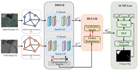
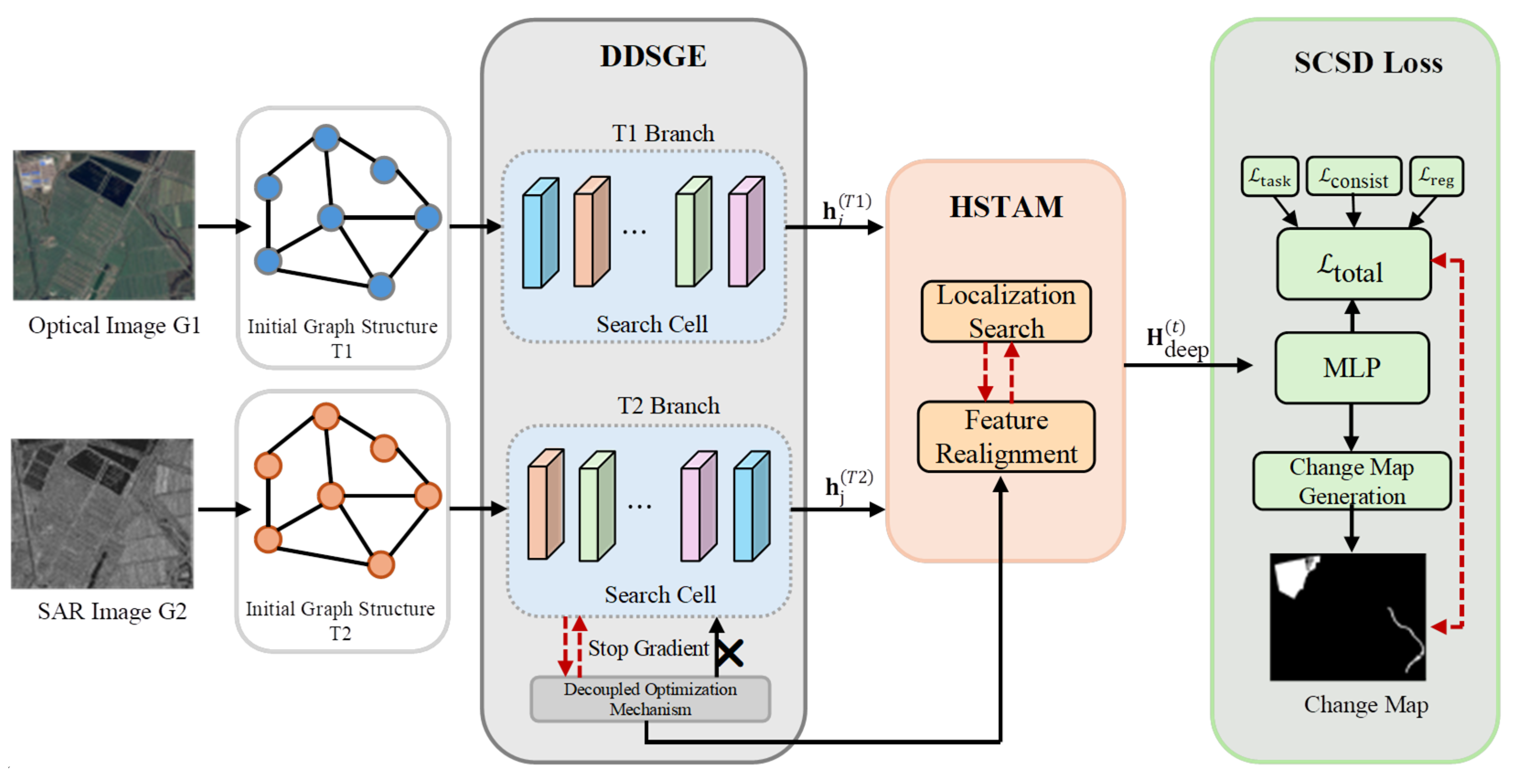
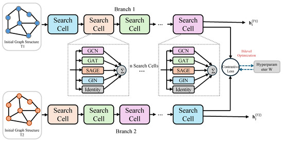
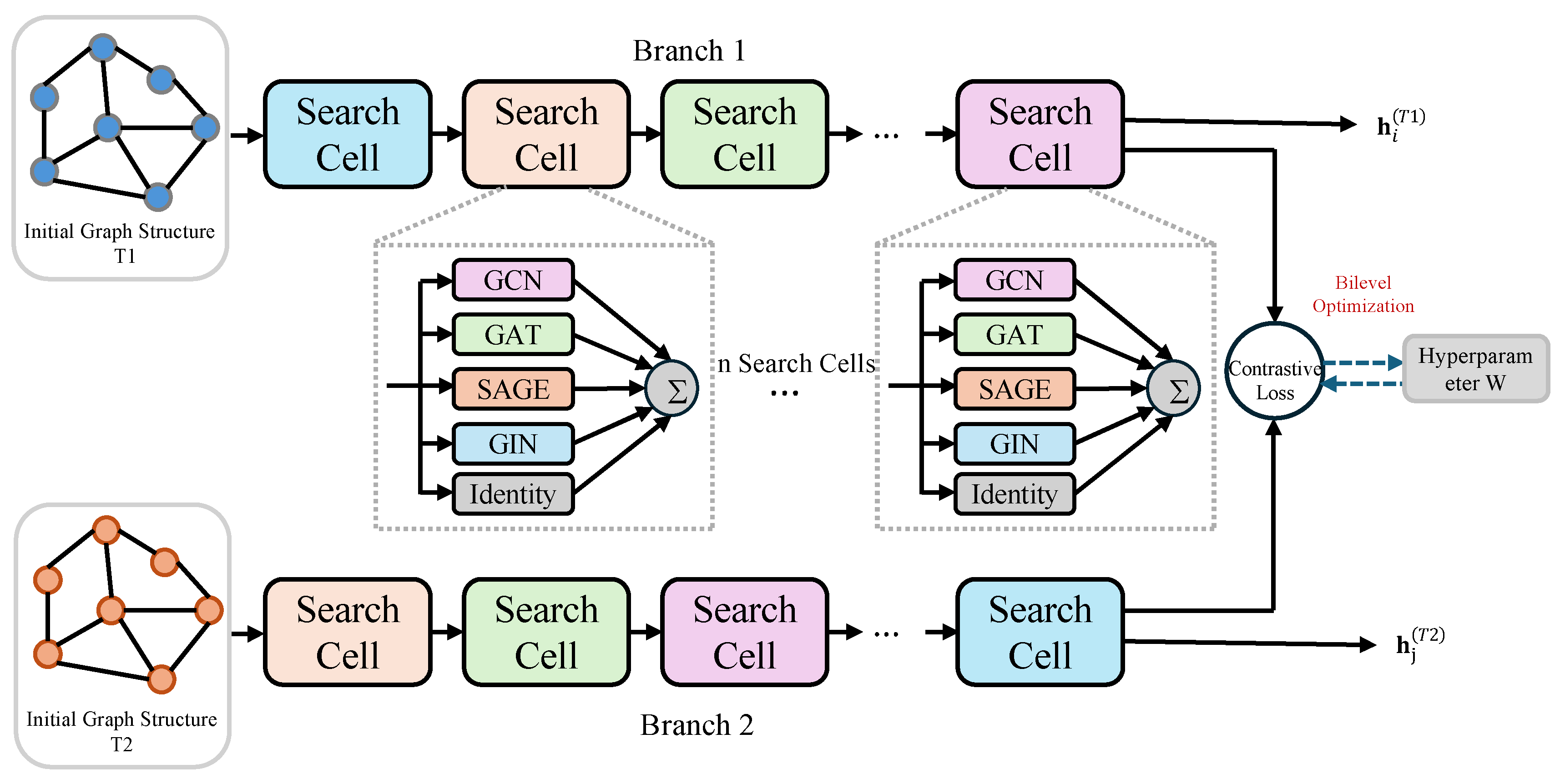
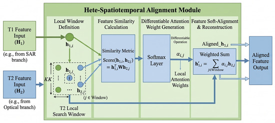
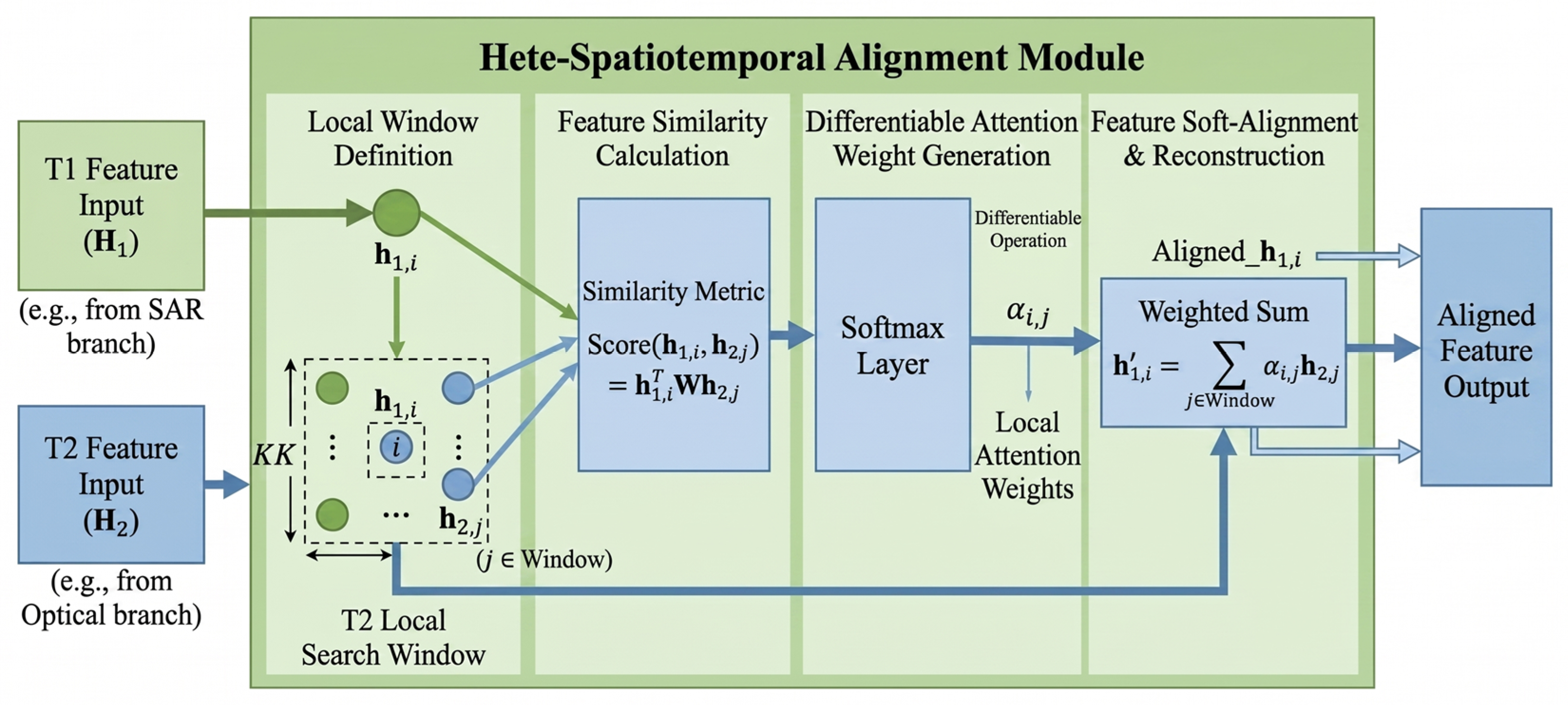
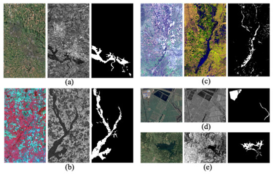
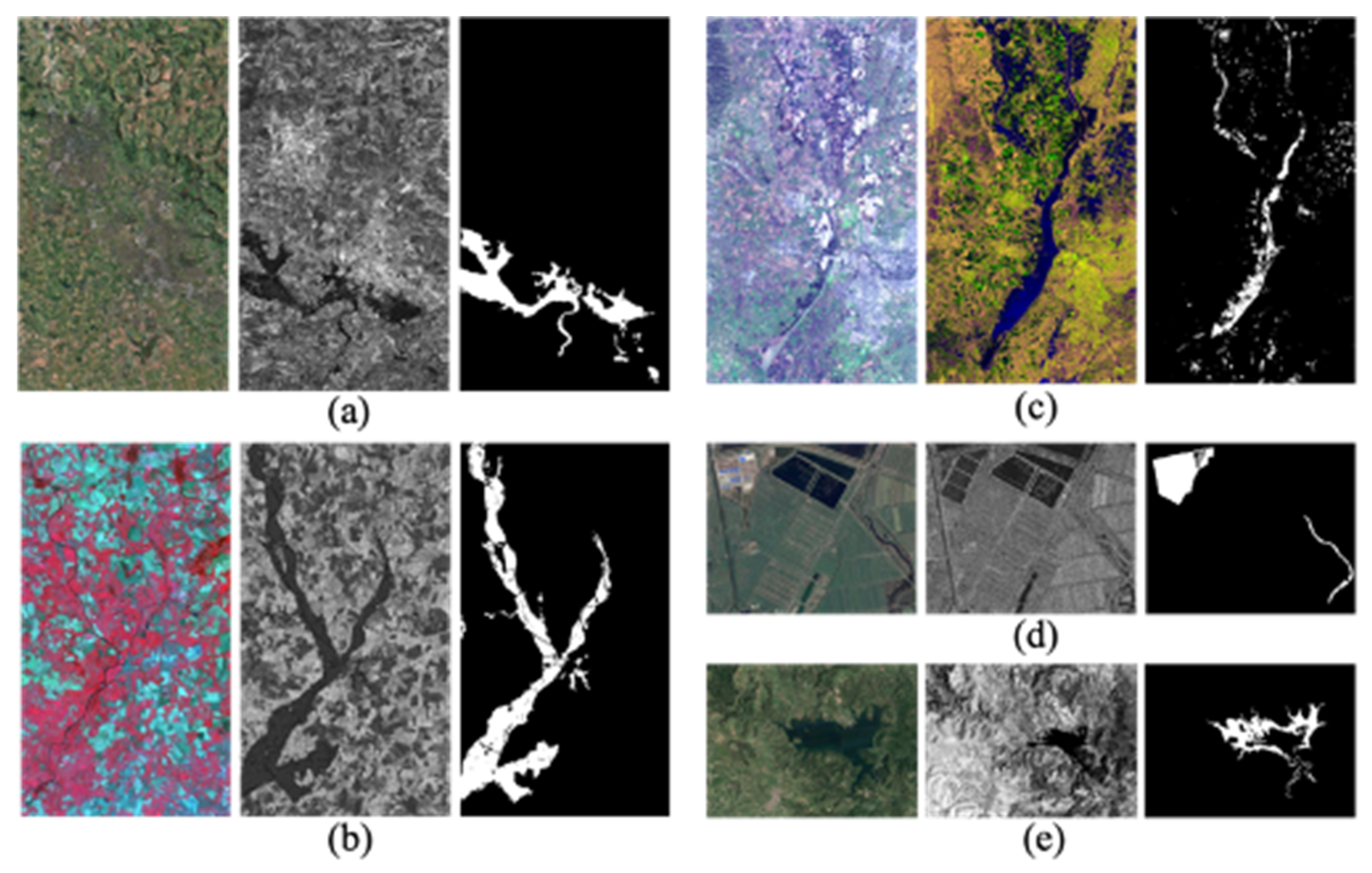
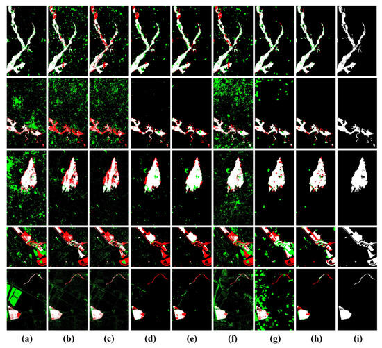
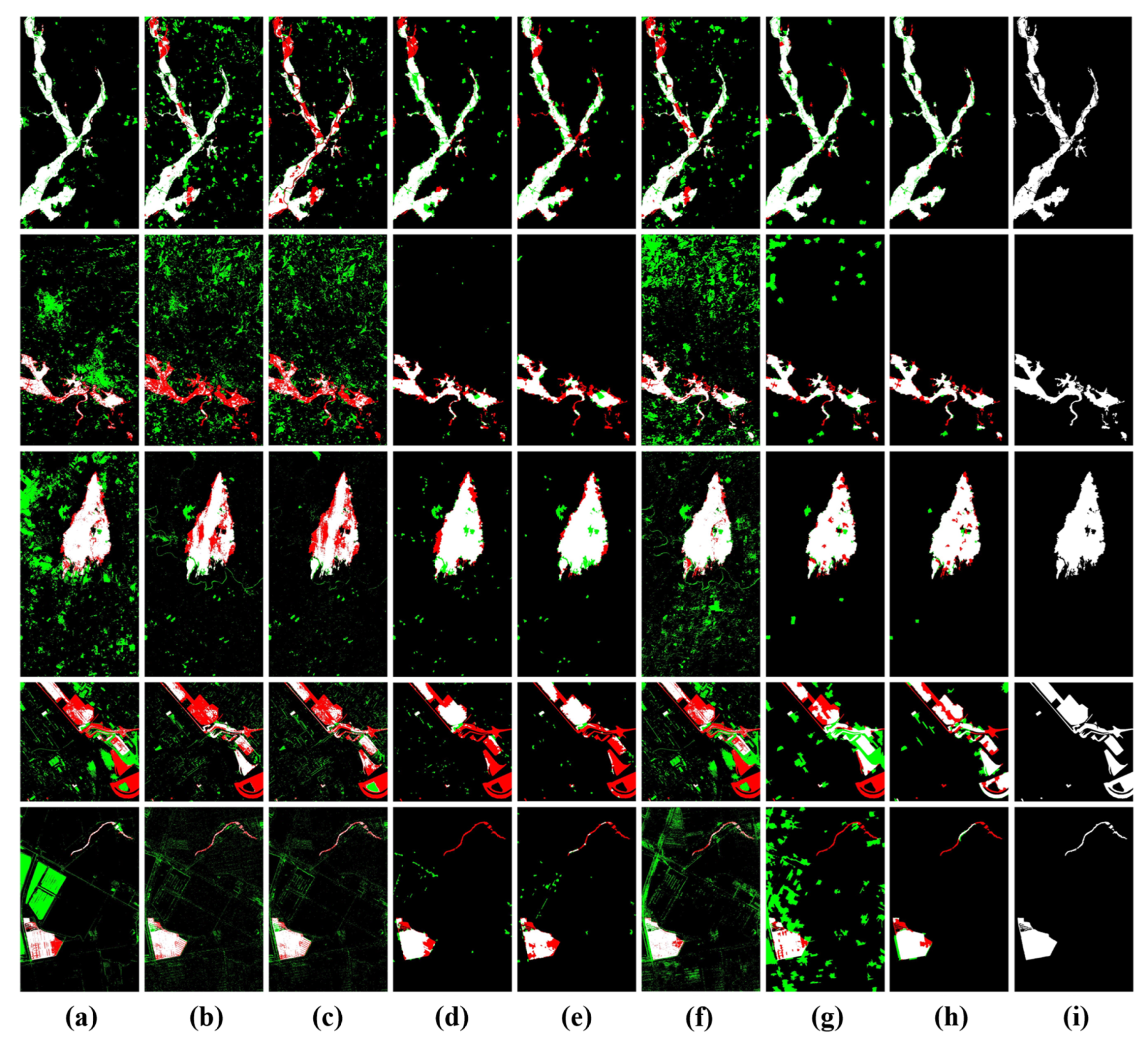
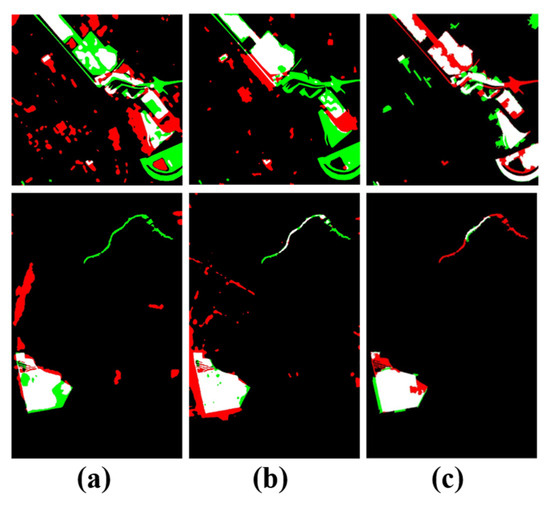
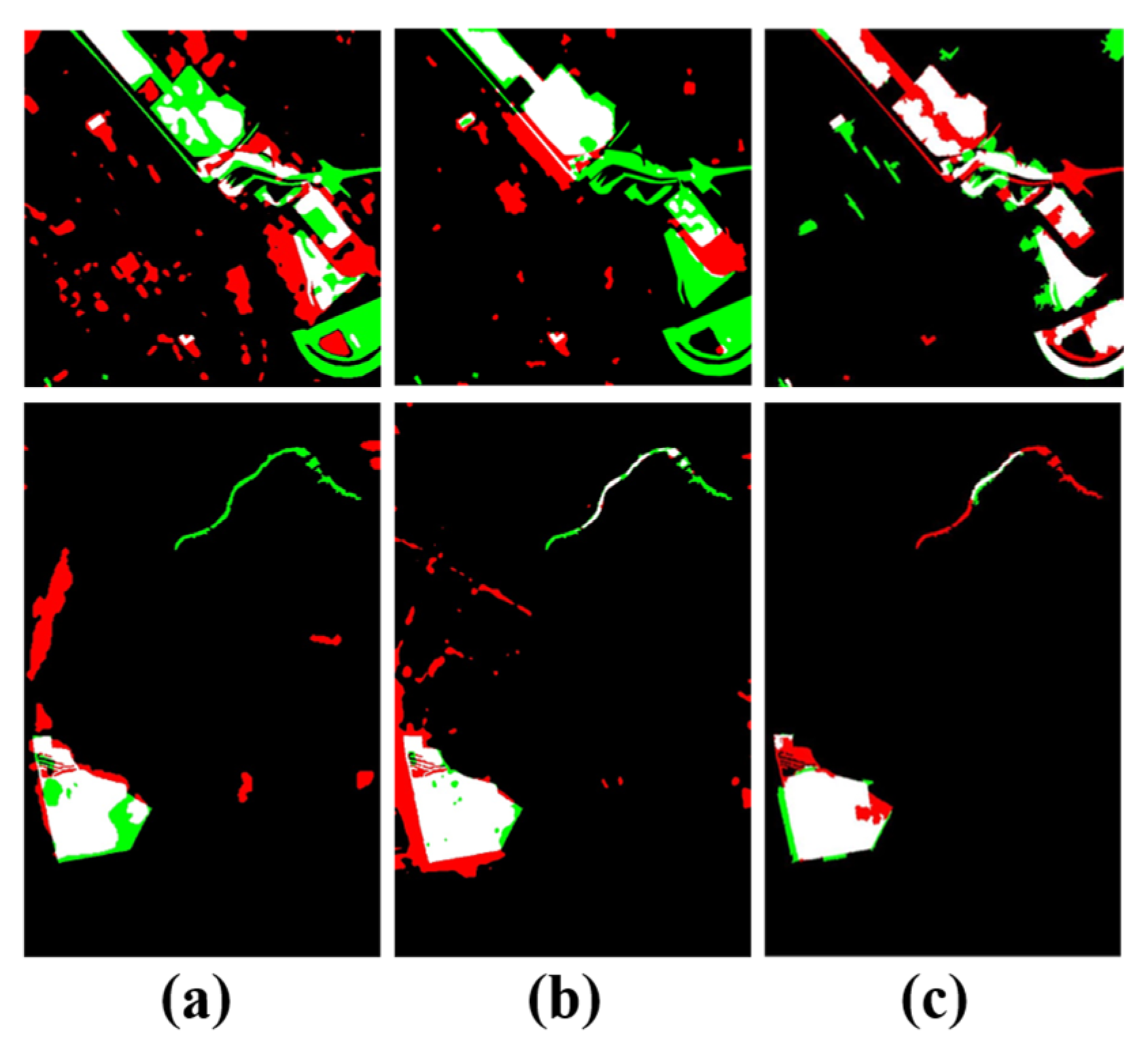
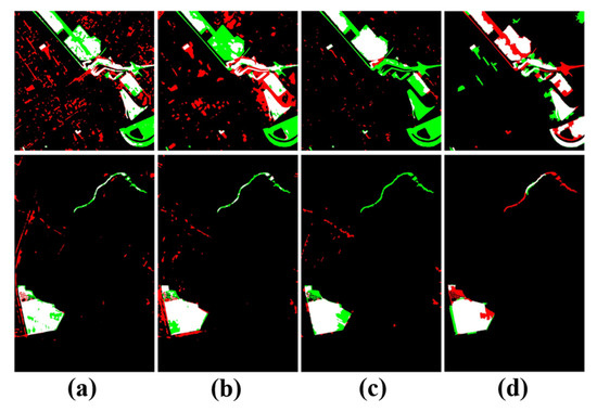
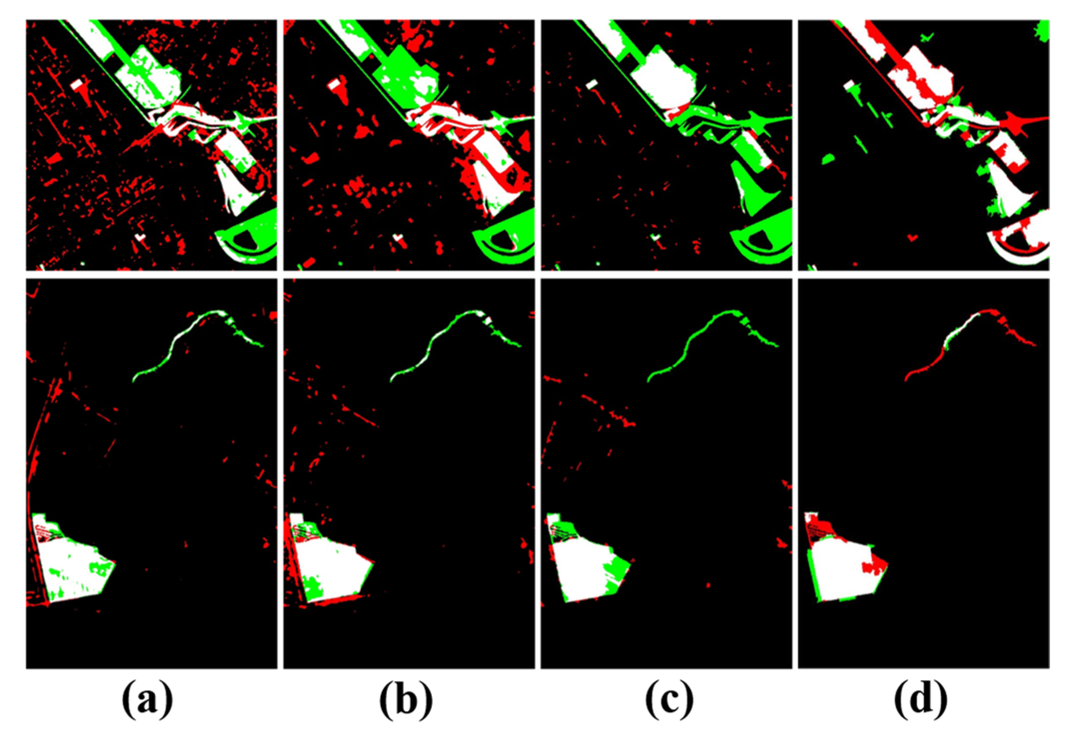

Disclaimer/Publisher’s Note: The statements, opinions and data contained in all publications are solely those of the individual author(s) and contributor(s) and not of MDPI and/or the editor(s). MDPI and/or the editor(s) disclaim responsibility for any injury to people or property resulting from any ideas, methods, instructions or products referred to in the content. |
© 2026 by the authors. Licensee MDPI, Basel, Switzerland. This article is an open access article distributed under the terms and conditions of the Creative Commons Attribution (CC BY) license.