


Highlights
What are the main findings?
- Automated selection methods that read a model’s outputs (uncertainty sampling, self-training, label propagation, and random selection) plateau well below dense supervision on ISPRS Vaihingen, even when an entropy oracle receives ground truth answers at up to 100 times the budget.
- An expert clicking confidently incorrect pixels, at most one per class per frame per iteration and with no auxiliary machinery, reaches 99.6% and 96.9% of the dense mIoU on ISPRS Vaihingen and BsB Aerial.
What are the implications of the main findings?
- Automated acquisition rules cannot find a model’s confident errors in its own outputs; a human inspecting the prediction overlay supplies exactly this missing signal, making expert clicks a sufficient replacement for the label-expansion machinery of prior pipelines.
- Segmentation models can be trained and maintained at a small fraction of the dense annotation effort (14 to 24 times fewer pointing actions), supported by the open-source iSAGE platform.
Abstract
Training semantic segmentation models is especially costly in remote sensing, since most problems require a new dataset as targets vary with resolution, sensors, and region. Approaches to reduce this cost are increasingly common, but most add machinery that expands few labeled pixels into a denser training signal using the model’s own predictions, where a confident prediction looks the same whether it is correct or incorrect. The hypothesis here is that these confident errors are the most valuable pixels to label, and that a human examining the image can identify them directly. We propose iSAGE (Iterative Sparse Annotation Guided by Expert), an open-source framework in which the annotator clicks confident errors in the prediction overlay, the clicks train the model under an error-weighted loss, and the updated model surfaces the next errors, with no automatic label expansion at any step. With at most one labeled pixel per class per frame per iteration, iSAGE recovers 96.9% of dense performance on BsB Aerial (74.79% mIoU from 0.040% of the pixels) and matches the dense baseline on ISPRS Vaihingen (76.65% vs. 76.93% from 0.011% of the pixels), surpassing published weakly supervised methods by nearly 4 mIoU points. Four automatic selection strategies run through the same loop plateau 7.3 to 14.4 points below iSAGE, and raising their budgets far higher does not close the gap; in a 35-method comparison, iSAGE is the only iterative human-in-the-loop framework without automatic label generation.
1. Introduction
How much data is needed to train computer vision models? Although the answer is task-, domain-, and target-dependent, the prevailing assumption is that extensive labeled data is a prerequisite. This belief has been reinforced by large-scale benchmark datasets such as Common Objects in Context (COCO) [1], Cityscapes [2], and ImageNet [3], which have fueled model-centric progress in deep learning through extensive experimentation and architectural innovation [4,5,6].
However, models in production demand more than benchmark-style labeling: (1) speed: Cityscapes reports 1.5 h of expert annotation per high-resolution urban scene [2], and MS-COCO took over a year and a half of collaborative effort [1]; (2) flexibility: dense datasets are hard to audit or extend, since adding a new class means revisiting every training image to insert the label; and (3) quality: dense annotation forces decisions on every pixel (including the ambiguous ones), introducing annotator biases (or errors) into the training signal. Remote sensing sharpens this problem because models trained on one sensor (multispectral, hyperspectral, or SAR), platform (satellites or UAVs), or geography rarely transfer to another, so nearly every problem requires its own dataset [7,8,9,10].
Cost-reduction strategies fall into three families, none of which removes the human from the loop. Foundation models (SAM [11], CLIPSeg [12]) segment from prompts but do not assign class labels in specialized taxonomies, and even when used as labeling shortcuts, they produce imprecise boundaries and miss small objects in medical imaging [13], fine-structure scenes [14], and remote sensing [15], limitations that the SAM2 paper [16] itself acknowledges. Few-shot methods [17,18] require meta-training on similar tasks, which is rare in specialized domains. The third family iterates on the target dataset by reading model predictions: weak supervision propagates sparse pixels through heuristics [19,20,21], active learning selects by uncertainty [22,23,24], pseudo-labeling reuses high-confidence predictions [25,26], and interactive frameworks combine human feedback with algorithmic label expansion [27,28,29].
These output-reading approaches differ in who produces the mask (human, heuristic, or model) but share the same input: the model’s predictive distribution. Acquisition rules based exclusively on the predictive distribution of a single model cannot distinguish a confidently incorrect prediction from a confidently correct one when their predictive vectors are identical, yet these pixels may carry corrective supervision that uncertainty-based selection does not prioritize. This information limitation motivates an external observer who can compare the prediction against the visual evidence in the image. Closing this gap requires both a conceptual move and the infrastructure to test it end-to-end. Yang et al. [29] came closest on the conceptual side by observing confident errors in a domain adaptation setting, but their response layered more machinery on top (staged acquisition, pseudo-label densification, consistency regularization, and domain-adaptation supervision) rather than testing whether the observation alone was enough. Concurrent work [30] reports the same confident-overlap phenomenon but addresses it through output-space correction, staying within the same input regime. On the infrastructural side, the experiment requires annotation UX, prediction overlays, record format, mask generation, training pipeline, and reproducibility tooling to live in one environment. Existing annotation tools (CVAT, Labelbox, and V7) stop at labeling, and existing training frameworks assume dense masks as input, so anyone running the experiment end-to-end would have to connect these stacks by hand at every iteration.
This paper proposes iSAGE (Iterative Sparse Annotation Guided by Expert), an integrated framework that fills both gaps, with the following contributions:
- A blind spot of output-reading acquisition. We show that four families of methods built on output-reading acquisition functions (uncertainty sampling, self-training, label propagation, and random selection) have a ceiling well below dense supervision, plateauing at 62.25 to 69.35 mIoU on ISPRS Vaihingen against 76.93.
- The human solution. We propose a human-in-the-loop framework that targets this blind spot directly, with no additional machinery and a restrictive budget of at most one labeled pixel per class per frame per iteration, reaching near-dense performance (99.6% and 96.9% of the dense mIoU on ISPRS Vaihingen and BsB Aerial). To the best of our knowledge, no prior work has run this experiment, and among the 35 methods surveyed, this is the only iterative human-in-the-loop configuration with no output-reading mechanism.
- iSAGE. The open-source platform couples inspection, annotation, record-keeping, and retraining in one environment, which no existing tool provides and without which the loop above cannot run. It extends to new domains through preprocessing and encoder choices, and every experiment in this paper was produced on it.
The paper is organized as follows. Section 2 reviews related work. Section 3 presents the iSAGE framework and its software platform. Section 4 describes the experimental protocols. Section 5 reports the results, including the controlled comparisons against output-reading baselines. Section 6 discusses implications and positions iSAGE in a 35-method comparison landscape. Section 7 concludes.
2. Related Work
iSAGE is positioned against three families of prior work: sparse and weak supervision, active learning, and interactive human-in-the-loop frameworks.
2.1. Sparse and Weakly Supervised Semantic Segmentation
Weak supervision strategies reduce labeling burden by replacing dense masks with less detailed annotations: image-level labels [31,32], bounding boxes [33], scribbles [34], class activation maps, and selected slices in volumetric data [35]. Sparse supervision is a stricter subset, providing only a few annotated pixels per image (typically below 1–5% [19,20,23,36]), and has been applied to medical imaging [37,38,39,40], remote sensing [20,41,42,43], and natural images [19,34].
How these sparse annotations reach a dense training signal divides the field into two strategies. Enhancement keeps the annotations sparse but compensates through architectural choices: Conditional Random Fields impose spatial coherence on predictions, either as post-processing or integrated modules [20,44,45,46], and custom losses weight the gradient contribution of labeled versus unlabeled pixels [36,37,47,48,49]. Label expansion generates pseudo-labels from sparse seeds through CRF-based refinement [50], GAN-based generation [51], student-teacher consistency [48], and, more recently, foundation models such as SAM [11] and CLIPSeg [12] that produce class-agnostic masks for downstream category assignment. Pseudo-labeling approaches typically mitigate the confirmation-bias risk through confidence thresholds, regularization, or ensemble validation [49,52,53]. The pattern persists in recent remote-sensing work: point-driven networks still densify their seeds through expansion modules [54,55], and SAM-adapted pipelines constrain the resulting pseudo-labels with uncertainty and consistency filters [56]. Whether through enhancement or expansion, the supervision signal that ultimately trains the model is generated algorithmically from the sparse seeds rather than supplied by the annotator directly.
2.2. Active Learning for Semantic Segmentation
Active learning reduces annotation effort by selecting which samples or regions a human annotates next, then refining the model after each iteration [57]. For semantic segmentation, acquisition functions score candidate samples along two main axes: uncertainty (entropy, margin, or model disagreement) and diversity/representativeness (coverage of the input distribution), often combined with task-specific signals such as loss prediction, multi-criterion scoring, simulation-before-annotation, or Bayesian decomposition of pixel-level uncertainty [58,59,60,61,62,63,64,65,66]. Recent work evaluates whether sparse annotations achieve comparable performance to dense supervision in this setting: Kellenberger et al. [23] showed that labeling less than 0.5% of a dataset could outperform fully supervised models in object detection when annotations are carefully selected; Li et al. [28] proposed HAL for few-shot segmentation with point-based annotations and iterative correction; Siddiqui et al. [67] introduced ViewAL for 3D scene annotation through viewpoint-based selection; and similar principles extend to point cloud segmentation [68].
A common assumption across uncertainty-based acquisition functions is that model uncertainty is a reliable proxy for informativeness. This assumption breaks down in two directions: a confident incorrect prediction registers no uncertainty, and a highly uncertain boundary pixel may contribute little new information about the semantic task. Mukhoti and Gal [69] found that the mapping between uncertainty and correctness in Cityscapes segmentation requires careful measurement rather than being self-evident; Gustafsson et al. [70] showed that deep ensembles improve over MC-dropout but still suffer calibration error under synthetic-to-real domain shift; and a recent benchmark of deep active learning concluded that many uncertainty-based methods barely outperform random selection [71]. These findings frame the limit of uncertainty-based acquisition. Confident errors register low uncertainty by definition, and so escape selection rules that query by uncertainty.
2.3. Interactive Human-in-the-Loop Frameworks for Semantic Segmentation
Human-in-the-loop (HITL) machine learning takes two distinct forms in computer vision [72,73,74]. Inference-time HITL refines individual predictions through user clicks or extreme points without altering the model [75,76,77]. Training-time HITL contributes to training supervision via labeled queries or coupled acquisition-and-correction loops, which is the focus of this section. iSAGE belongs to the latter. Inference-time methods and acquisition-only active learning lie outside its design space.
Several training-time HITL frameworks target semantic segmentation specifically. DIAL [27] combines uncertainty-driven sampling with region-based refinement and direct user feedback, using user input to compensate for cases where model uncertainty misses informative pixels. HAL [28] implements interaction loops for real-time correction of segmentation masks based on user clicks, using a dual-network mechanism that consolidates sparse clicks into dense masks for training. EasySeg [29] combines a See-First-Ask-Later (SFAL) acquisition strategy, which identifies obvious model errors before querying uncertain pixels, with an ISS-Net pseudo-label generator under a domain adaptation setting, reporting performance above its fully supervised baseline at a fraction of the annotation cost. Across these frameworks, sparse human input reaches a dense training signal through an algorithmic expansion step, whether patch retraining (DIAL), dual-network consolidation (HAL), or pseudo-label generation (EasySeg).
The inspection step itself, a human viewing the model’s predictions overlaid on the image and correcting visible errors, has precedents outside this family. In RootPainter [78] and Deep Interactive Learning [79], corrective annotations retrain the model directly, with no acquisition function or label expansion. In both, however, each correction is a densely painted region, so the annotator still delineates extents and boundaries at every correction. iSAGE keeps the inspection workflow but reduces each correction to a single labeled pixel, which removes the boundary decision from the annotation act.
More recent frameworks extend this pattern with foundation-model pseudo-labels. ALC [80] refines SAM-generated labels through human correction queries, and A2LC [81] automates the correction decision. In remote sensing, PointSAM adapts SAM to point supervision through self-training with prototype-based regularization [82]. Because these pipelines operate on SAM-generated regions, the training signal flows through boundaries the foundation model drew. These boundaries are imprecise on specialized domains such as medical imaging [13], fine-structure scenes [14], and remote sensing [15], and the SAM2 paper [16] acknowledges the issue itself. Making SAM usable at scale additionally requires engineering for coverage and cross-tile consistency [83]. iSAGE removes this dependency: clicks land only on pixels of visually unambiguous class, and the click itself never asks the annotator for a boundary decision.
3. iSAGE Framework
iSAGE is a framework for semantic segmentation in which sparse human clicks drive an iterative training loop. The annotator identifies pixels where the current model is confidently wrong at each iteration. The growing record of (coordinate, class) tuples, stored as a JSON file, is converted deterministically into training masks. The Error-Weighted Dice Loss (EWDL) then trains the next iteration with those clicks amplified relative to already correct predictions. No propagation, pseudo-labeling, or other algorithmic densification step sits between the click and the gradient. An integrated platform hosts inspection, annotation, retraining, and dataset maintenance as a single workflow. The following four subsections describe the click-based annotation, the iterative refinement loop, EWDL, and the platform. Figure 1 overviews the iteration cycle.
Figure 1.
iSAGE workflow: Iterative annotation, training with EWDL, and user-decided stopping. Solid arrows follow the data through one iteration; the blue dashed box marks the human in the loop, who supplies the point annotations and the quality check; green and red boxes mark the start and the user-decided stop.
3.1. Sparse Annotations
Sparse annotation labels only a subset of pixels in each frame. The rest are treated as ignore during training. In iSAGE, each annotation corresponds to exactly one pixel. The user clicks on a location in the image, and the software records the coordinate along with the selected class label, with no region expansion, bounding box, or area selection. The resulting set of tuples constitutes the complete training supervision, and the dataset produced by iSAGE is the annotation file itself.
The choice of a single-pixel click as the basic annotation unit is deliberate. Scribbles and sparsely drawn polygons also reduce the total pixel count relative to dense masks, but points have a property that these alternatives do not share: per-decision auditability. Each point annotation is a single (coordinate, class) tuple, individually verifiable by returning to the pixel and independently correctable at the record level (remove one JSON entry). Scribbles bundle multiple pixel-level decisions into a single primitive, so errors in part of the scribble are not easily localized or corrected. Polygons reintroduce boundary decisions, where labels are intrinsically ambiguous, and annotator uncertainty becomes label noise; the training procedure cannot distinguish it from correct supervision. The point primitive therefore forces single-pixel granularity, which aligns with the workflow’s commitment to labeling only pixels where the class is visually unambiguous. Because each click contributes exactly one pixel regardless of object size, the annotator also balances class contribution independently of spatial extent, a second advantage that follows from the same primitive.
Formally, let I be an input image and be an annotation function that assigns class labels to pixels, where C is the number of classes, and label 0 denotes the background. Supervision, in sparse annotations, only considers a limited set of pixels , and A is undefined outside S, thus:
Pixels with value act as an ignore mask and contribute zero gradient. In the implementation, the ignore value is stored as C, the first integer outside the label range. This regime does not restrict what the network sees, only which pixels it is penalized on. The gradient from each labeled pixel updates all weights that influenced its prediction, so the network’s spatial inductive biases generalize the class signal to visually similar pixels, and shape and boundary information emerges from the learned representation rather than from explicit boundary annotation.
For binary segmentation (), the labels reduce to , with 1 for the foreground and 0 for the background. In the multiclass scenario, labels correspond to the object classes.
3.2. Iterative Error-Driven Refinement
The iSAGE cycle improves the model by annotating regions where predictions are wrong. Error-focused supervision concentrates each new label on a region the current model gets wrong rather than on a randomly chosen pixel. Algorithm 1 describes this iterative process.
| Algorithm 1 Iterative Error-Driven Refinement for Sparse Annotations |
|
The initial set is collected on the raw images without a prediction overlay, since no model has been trained yet (in the same interface and under the same budget), choosing pixels for class clarity. From iteration 1 onward, the operator selects new points from the errors visible in the prediction overlay; the model is retrained on the expanded set, and the procedure repeats for N iterations.
Operationally, confidently wrong means a pixel where the class displayed in the argmax overlay differs from a class that is visually unambiguous in the imagery, and no confidence map, threshold, or uncertainty estimate takes part in the selection. The name refers to the model’s side. Such errors typically carry low output uncertainty, so output-reading rules do not prioritize them. A class omitted entirely from a frame stays annotatable, since the missed objects appear painted with another class’s color and are clicked with the true label.
The experiments in this paper deliberately adopt the smallest possible supervision budget, at most one pixel per class per frame per iteration, as an adversarial test of the workflow. In practice, iSAGE places no fixed limit on annotation density, and the annotator decides how many points each frame requires.
3.3. Error-Weighted Dice Loss
Standard loss functions treat all labeled pixels equally during training. Under sparse annotation, this can be problematic: the model receives limited supervision, and correct predictions (often the majority) dominate the gradient signal, while misclassified pixels receive insufficient attention. The proposed Error-Weighted Dice Loss (EWDL) addresses this imbalance by amplifying the contribution of incorrectly predicted pixels.
Formulation
Let denote the ground truth label at pixel x, and let be the predicted probability for class c. The standard Dice loss for class c is
where is the one-hot ground truth for class c, and ensures numerical stability.
EWDL introduces a per-pixel weight based on prediction correctness. For each labeled pixel , a binary indicator captures whether the predicted class matches the annotator-provided ground truth:
The weight assigned to each pixel depends on this correctness,
where is the error penalty factor. When , EWDL reduces to standard Dice loss. The indicator is recomputed at every forward pass and treated as a constant with respect to the network parameters: the argmax is non-differentiable, and no gradient propagates through . Because the Dice numerator and denominator couple all pixels, the weight does not multiply each pixel’s gradient by exactly ; it increases the relative influence of misclassified pixels in the class-wise ratio, shifting the optimization toward the model’s mistakes.
The weighted Dice loss for class c becomes:
For multiclass segmentation with C classes, the total loss averages across all classes:
All summations over x above run over the labeled set S defined above. Unlabeled pixels contribute zero weight and zero gradient, consistent with the ignore mask behavior of standard sparse training. Three implementation details complete the specification. The sums pool the labeled pixels of all images in the batch, so the Dice ratio is computed per class over the batch rather than per image, and the class average includes the background class. The weights are rescaled to sum to the number of labeled pixels; the Dice ratio is homogeneous in w, so the rescaling changes nothing beyond the smoothing and serves numerical stability ( throughout). A class with no labeled pixels in the batch contributes only through predicted probability mass assigned to it at the labeled pixels, and with , its term vanishes when that mass is zero. The binary tasks apply the same weighting to a single foreground Dice term.
3.4. Software Platform
The platform is the experimental instrument that makes the alternative to output-reading supervision testable end-to-end. Without a single environment coupling prediction overlay, click annotation, record persistence, and retraining, the iterative loop fragments into ad-hoc stitching across tools, and the experiment ceases to run at research scale. Figure 2 shows the annotation interface, with the model’s prediction overlaid on the image for click-based correction. The interface can also display a ground truth overlay for auditing when reference labels exist; the experiments reported here did not use it.
Figure 2.
Annotation interface with the prediction overlay on training images. Center: the current frame with the prediction overlay and the click points; left: class selection and display settings; right: mini-map of the original image, image information, and the running count of annotation points.
The platform comprises four subsystems:
- Annotation interface: Hosts prediction overlay and click-driven annotation.
- Record storage: Persists every decision as JSON.
- Session layout: Packages each iteration as a reproducible snapshot.
- Training backend: Closes the loop with EWDL-supervised retraining.
The platform is domain-agnostic by construction: any dataset with standard image formats and enumerable classes runs through the pipeline, requiring only domain-specific preprocessing and encoder choice. The training backend itself is pluggable. The default implementation uses Segmentation Models PyTorch (version 0.4.1) [84], built on PyTorch [85], and the released platform drives the same workflow from a Jupyter notebook [86], a command-line interface, or the Python (version 3.11) API. Any trainer that reads iteration_N/masks/ and writes the corresponding model checkpoint and predictions can replace the default without touching the annotator or the record format.
The training loop does not read the JSON files directly. The annotation record is converted to dense per-image masks by a standalone mask generator, and the training dataloader consumes those masks. This separation has three consequences: (1) the JSON record is a self-contained audit trail of human decisions and can be versioned, diffed, shared, or replayed without running the training pipeline; (2) mask generation is reproducible: given the same JSON files and the same converter, two practitioners obtain identical training masks; (3) the dataset is portable: the JSON files plus the converter are sufficient to reconstruct the supervision signal, without requiring the annotation tool or its UI state. Together, these properties make the annotation record a complete, portable, auditable dataset rather than a sparse input to a densification pipeline.
4. Experiments
4.1. Experimental Setup
All experiments use the same U-Net with EfficientNet-B7 encoder. The fixed architecture isolates annotation-strategy effects from model variability, and since iSAGE’s predictions also guide annotation, architectural changes would shift point-selection trajectories across iterations. A cross-architecture validation (Section 4.3) retrains three additional configurations on the final annotation record, testing whether the sparse dataset produced by the loop replicates its result across backbones. The framework is architecture-agnostic by design: any model in the Segmentation Models PyTorch library [84] can replace it. Table 1 lists the hyperparameters. All training ran on a single NVIDIA GeForce RTX 4090. The iSAGE code and configuration files are released at https://github.com/osmarluiz/iSAGE (accessed on 27 August 2026) and archived at https://doi.org/10.5281/zenodo.20596185.
Table 1.
Training configuration for iSAGE experiments.
Performance is evaluated using IoU, F1-score, precision, and recall per class. iSAGE reports the final-epoch model, since the sparse-click setting presupposes no labeled data. Dense supervision baselines use the best-validation checkpoint per standard practice. On both datasets, this validation signal comes from the held-out evaluation partition itself (an asymmetry that can only favor the dense baselines), so the reported iSAGE-to-dense comparisons are conservative. Final-iteration and ablation values on the multiclass task, and the final-iteration iSAGE and dense values on Vaihingen, are means over five training seeds, and per-iteration trajectories come from the single interactive annotation session, whose clicks are collected once. Random-selection results on the multiclass task are means over five independently seeded chains sharing iSAGE’s iteration-0 bootstrap.
The compared frameworks report annotation budgets as pixel fractions, clicks, or region counts, and none measures annotation time [24,27,29,89,90,91], which conflates concentration, fatigue, and interface fluency. Measuring time credibly would also require timing the dense workflow on the same imagery under the same conditions, a controlled study in its own right. Annotation effort is therefore reported here as the fraction of labeled training pixels, the standard cost metric of this literature and one exactly reproducible from the annotation record.
The fraction measures supervision density rather than human work, so effort is additionally counted in pointing actions, the number of times an annotator marks a location. For iSAGE, this is the click count. For dense annotation, which delineates polygons, it is the number of vertices needed to reproduce the ground truth. Each training mask is binarized per class (clutter excluded), matching how an annotator outlines one class at a time, boundaries are extracted as outer contours plus holes, and each closed boundary is simplified with the Douglas–Peucker algorithm [92] at tolerances of 2 and 1 pixels, both stricter than the 3-pixel boundary erosion the ISPRS evaluation protocol applies to discount boundary uncertainty [7]. The vertex count is an idealized lower bound, assuming optimal placement and no corrections, and the exact count of the unsimplified boundaries is kept as a reference point.
4.2. Datasets
Two complementary remote sensing datasets serve distinct roles. BsB Aerial, curated by the authors, is the controlled laboratory for comparisons against dense supervision, random selection, and alternative losses that a public benchmark cannot support. ISPRS Vaihingen is the external benchmark for comparisons against published methods and for the four controlled output-reading baselines (oracle entropy, self-training pseudo-labels, CRF-based label propagation, uniform random). The two datasets vary across geography (Brazil vs. Germany), spectral composition (RGB vs. IRRG), and spatial resolution (0.24 m vs. 0.09 m).
4.2.1. BsB Aerial
BsB Aerial uses an aerial ortho image of Brasília, Brazil, at 0.24-m spatial resolution and three spectral bands (Red, Green, Blue), located at approximately 15°47′32″S latitude and 47°52′10″W longitude. The image was divided into non-overlapping 256 × 256 pixel frames, ensuring each annotated point appears in only one frame and preventing duplicated annotations. The study used 1250 patches: 1000 for training and 250 for held-out testing. No separate validation split enters the protocol. iSAGE presupposes that no labeled pool exists beyond the clicks, and the dense baselines’ checkpoint selection draws its validation signal from the 250 held-out patches. The ortho image and class definitions come from the authors’ earlier releases of the dataset [9,93,94]; the frame selection used in this study was drawn anew.
The four BsB Aerial classes are used as an experiment in class-type isolation. Each was selected to test iSAGE on a distinct combination of geometry, boundary, and texture:
- Small discrete objects (cars): Rigid geometry, sharp boundaries, low spatial frequency.
- Linear connected structures (roads): Elongated, with mixed boundary regimes and frequent occlusion.
- Large polygonal structures (buildings): Rectilinear, with sharp boundaries and rich interior texture.
- Amorphous smooth-boundary regions (permeable areas): Irregular, with mixed textures and high intra-class variance.
Each category carries a characteristic failure mode for methods relying on model outputs or dense ground truth. Figure 3 shows one example of each.
Figure 3.
Examples of the four target classes: (A) buildings, (B) cars, (C) permeable areas, and (D) roads. Black squares outline the 256 × 256 pixel frames (0.24 m spatial resolution); scale bars indicate 10 m.
4.2.2. ISPRS Vaihingen
ISPRS Vaihingen [7] is a standard benchmark for urban semantic segmentation, with 33 aerial image tiles over Vaihingen, Germany, at 0.09 m spatial resolution and three spectral bands (near-infrared, red, green). Ground truth annotations cover six semantic classes: impervious surfaces, buildings, low vegetation, trees, cars, and clutter/background.
The test split follows the same 17-tile partition used by EasySeg [29], yielding 155 non-overlapping 512 × 512 test patches. Training uses 1000 non-overlapping 512 × 512 patches from the remaining 16 tiles, a 44% reduction relative to the 1784 patches used by EasySeg: this smaller training set is a deliberate constraint, not an advantage, kept consistent with iSAGE’s minimum-effort regime. The partition defines no validation tiles; the dense baseline’s checkpoint selection likewise draws its validation signal from patches of the test partition.
Training proceeds on five classes (impervious surfaces, buildings, low vegetation, trees, cars), excluding clutter. The exclusion follows from the class itself: clutter is a catch-all category whose contents differ between the training and test tiles of the EasySeg partition. Water bodies, for example, appear as clutter in the training tiles but not in the test tiles, so the class cannot be learned from the Vaihingen imagery alone, and every configuration evaluated here, sparse and dense alike, yielded zero IoU on it. EasySeg recovers clutter only because its Potsdam domain-adaptation signal supplies external dense supervision for the class, a mechanism iSAGE deliberately avoids. The exclusion applies identically to iSAGE and to the dense baseline trained under the same protocol, so it cannot favor iSAGE: the match-with-dense result is a ratio in which both terms share the five-class setting.
4.3. BsB Aerial Experiments
The BsB Aerial dataset was annotated by a single annotator, holding annotator identity constant across the controlled comparisons (EWDL vs. alternative losses, error-driven vs. random selection, sparse vs. dense supervision). External validation against an independent ground truth is provided by the Vaihingen experiments in Section 4.4. The protocol comprises seven experiments:
- Binary experiments. Four independent tasks, one per class, to isolate per-class convergence dynamics from class competition and observe how each visual category evolves across iterations. Each task runs for 5 iSAGE iterations after the initial seed.
- Multiclass experiment. Joint training over all four classes plus background, under the same 5-iteration protocol, to test whether multiclass supervision changes per-class behavior relative to the binary baselines.
- Dense supervision upper bound. Models trained with dense ground truth masks under the same architecture, providing the performance ceiling iSAGE is compared against.
- Random selection baseline. The iterative protocol with randomly selected sparse annotations in place of error-driven selection, controlling for whether iSAGE’s gain comes from sparsity per se or from error-targeting. This baseline is the without-expert-guidance control: it shares the pipeline, budget, loss, and training schedule, differing only in who selects the pixels.
- Alternative loss functions. EWDL compared against Binary Cross-Entropy (BCE), Focal, and Dice losses on the binary tasks and against Cross-Entropy (CE), Focal, and Dice on the multiclass task, on the iter-5 final annotation set, testing whether EWDL’s error-weighting actually contributes to iSAGE’s performance or a standard loss suffices.
- EWDL hyperparameter sensitivity. The error-penalty factor varied over {1, 2, 5, 10, 20} on the iter-5 set, multi-seed, to probe the loss’s stability around the chosen .
- Cross-architecture validation. Four model configurations (the primary U-Net + EfficientNet-B7 plus U-Net + ResNet-101, DeepLabV3+ + ResNet-50, and SegFormer + MiT-B2), each paired with a matched dense-supervision baseline and trained under the identical five-seed protocol on the iteration-5 annotation set, covering three decoder families (encoder-decoder, atrous spatial pyramid, hierarchical transformer), to test whether the annotation record transfers across backbones.
4.4. ISPRS Vaihingen Experiments
The Vaihingen experiments comprise two groups: an external benchmarking block where iSAGE is run on Vaihingen and compared against published methods, and four output-reading baselines that re-run the iSAGE protocol with automated acquisition mechanisms in place of the human annotator.
4.4.1. External Benchmarking
- iSAGE on Vaihingen. The complete iSAGE pipeline (sparse seed annotations, error-driven refinement over 5 iSAGE iterations, EWDL training) is applied to Vaihingen under the same per-iteration budget used throughout (at most one labeled pixel per class per frame), accumulating to at most six labeled pixels per class per frame over the five iterations plus the seed. Performance is compared against published methods on EasySeg’s [29] 17-tile test partition.
4.4.2. Output-Reading Baselines
Four automated acquisition mechanisms are re-run under iSAGE’s protocol on Vaihingen, representing the dominant automated alternatives to human-in-the-loop supervision: uncertainty-based active learning [57,69], self-training with pseudo-labels [25,26], CRF-based label propagation [95], and uniform random sampling as a control. The goal is to test whether any of these can match iSAGE’s human-targeted signal. All four share iSAGE’s model, training schedule, and iter-0 seed annotations. Oracle entropy and uniform random keep the same per-iteration budget cap as iSAGE. The oracle selects per predicted class per frame, since an entropy rule can only rank pixels within classes the model predicts, while uniform random draws one pixel per ground truth class per frame, independently of the model’s outputs. Pseudo-labeling and CRF propagation have no per-iteration cap and expand the supervision set automatically across iterations. To rule out budget calibration and confidence-threshold calibration as the lever, the oracle is additionally evaluated at 10×, 50×, and 100× the per-class budget, and pseudo-labeling at confidence thresholds 0.90, 0.95, and 0.99.
- Oracle entropy [57,69]: At each iteration, the highest-entropy pixel per predicted class per frame is selected, with ground truth labels assigned at the selected coordinates. Tests whether the strongest possible uncertainty-driven acquisition, given ground truth answers at every query, can match iSAGE. The budget sweep at 10×, 50×, and 100× labels per class per frame reaches up to 0.95% of training pixels and tests whether budget alone closes the gap to iSAGE.
- Pseudo-labeling [25,26]: At each iteration, pixels whose predicted-class confidence exceeds a fixed threshold are converted to pseudo-labels and added to the supervision set. Tests whether self-confidence can expand sparse seeds into adequate supervision without human input. The threshold sweep at 0.90, 0.95, and 0.99 tests whether confidence calibration is the lever that closes the gap.
- CRF-based label propagation [95]: At each iteration, the model’s softmax outputs are refined by a DenseCRF with a Gaussian spatial pairwise term and a bilateral color-position pairwise term (pydensecrf defaults: Gaussian = 3, compatibility 3; bilateral = 80, = 13, compatibility 10; five mean-field iterations) before a confidence threshold matching the strongest pseudo-labeling configuration in the threshold sweep above is applied. Tests whether spatial smoothing of model outputs adds value on top of the best expansion baseline, isolating smoothing from threshold calibration.
- Uniform random: A control baseline that selects one pixel per ground truth class per frame, uniformly at random within that class’s region and independently of the model’s predictions. Tests whether any acquisition structure outperforms the simplest sampling.
5. Results
Results follow the structure of the experimental protocol (Section 4). The BsB Aerial subsection reports iSAGE performance on the binary and multiclass tasks, against the random and dense reference baselines, and across loss, , and architecture ablations. The ISPRS Vaihingen subsection compares iSAGE against published state-of-the-art methods on the shared 17-tile test partition and reports iteration trajectories for four output-reading baselines (oracle entropy, pseudo-labeling, CRF-based label propagation, and uniform random), with the structural interpretation reserved for Section 6.1.
5.1. BsB Aerial
On the four binary tasks, iSAGE reached final IoUs of 74.05 (car), 81.88 (road), 81.48 (building), and 88.17 (permeable area) at iteration 5 with annotation effort below 0.018% per task, recovering 95.0%, 97.4%, 95.1%, and 97.1% of the corresponding dense IoU (Table 2, Figure 4). Cars improved by +46.6 IoU between iterations 0 and 5 and still ended with the lowest absolute IoU (74.05 against a dense ceiling of 77.93). Permeable area improved by only 6.4 IoU and started highest.
Table 2.
Binary segmentation results on BsB Aerial. Per-class IoU, precision, recall, F1-score, and annotation effort (%). Underlined values are the best per column within each block; the dense-supervision row is set in bold italics as the upper bound.
Figure 4.
Visual progression of segmentation results across iSAGE iterations. Column labels 1–6 follow the annotation tool’s 1-indexed sessions and correspond to iterations 0–5 in the text; IoU values printed on panels are per-image, not dataset means.
On the multiclass task, iSAGE reached 74.79% mIoU and 84.83% macro F1 at iteration 5 with 0.040% cumulative annotation effort across all five classes, recovering 96.9% of the dense ceiling (77.17% mIoU) (Table 3). Per-class IoUs at iteration 5 were 88.72 (permeable area), 81.89 (building), 82.36 (road), 70.72 (car), and 50.27 (background).
Table 3.
Multiclass segmentation results on BsB Aerial. Macro metrics and per-class IoU (%). Underlined values are the best per column within each block. Iteration-5 iSAGE values and the loss-function panel are means over five training seeds (standard deviation at most 0.3 mIoU).
On the binary tasks, random selection reached final IoUs of 48.47 (car), 75.67 (road), 73.82 (building), and 86.69 (permeable area), with gaps to iSAGE of −25.6, −6.2, −7.7, and −1.5 IoU respectively (Table 2, Figure 5). Random selection saturated the budget cap on every frame, so its cumulative effort matched or exceeded iSAGE’s on every class.
Figure 5.
Qualitative comparison of final-iteration segmentation results. Columns: Ground truth, random selection, dense supervision, BCE, Focal, Dice, and iSAGE. IoU values printed on panels are per-image, not dataset means.
On the multiclass task, random selection plateaued at 69.11% mIoU at iteration 5, 5.68 points below iSAGE at matched annotation effort (Table 3).
On the four binary tasks (Table 2, bottom panels), EWDL and the alternative losses land within 0.6 IoU of one another on every class at the final iteration.
On the multiclass task, evaluated on the iter-5 annotation set (Table 4), landed within 0.16 mIoU of one another (74.63, 74.79, 74.66), with per- standard deviations of 0.19 to 0.33. (standard Dice) reached 73.37, and dropped to 72.18. Against alternative loss families under the same protocol (Table 3, bottom panel), EWDL () at 74.79% led Cross-Entropy (74.11 ± 0.09) by 0.68 points and matched Focal (, 74.66 ± 0.20) within one standard deviation (EWDL 74.79 ± 0.27).
Table 4.
EWDL hyperparameter sensitivity on BsB Aerial multiclass. Mean mIoU and per-class IoU (%) across 5 seeds under varying error-penalty ( recovers standard Dice). Bold marks the default setting; underlined values are the best per column. Standard deviations range from 0.19 to 0.33 mIoU.
Across the four backbones trained on the same iter-5 annotation set (Table 5, the means over five seeds), iSAGE reached 74.79 (U-Net + Eff-B7), 72.32 (U-Net + R101), 70.69 (DLV3+ + R50), and 71.86 mIoU (SegFormer + MiT-B2), recovering 96.9, 94.4, 94.1, and 95.7% of each architecture’s matched dense ceiling. Table 5 also lists each architecture’s parameter count and multiply-accumulate cost. A 100-epoch iteration with the primary configuration took about 30 min on BsB Aerial and about one hour on ISPRS Vaihingen (Section 5.2), so the six trainings of a full protocol were completed within a working day.
Table 5.
Cross-architecture validation on BsB Aerial multiclass with U-Net + EfficientNet-B7 (Eff-B7), U-Net + ResNet-101 (R101), DeepLabV3+ (DLV3+) + ResNet-50 (R50), and SegFormer + MiT-B2 backbones. mIoU and per-class IoU (%) for iSAGE (mean over five training seeds on the iteration-5 annotation set, identical training protocol across architectures; standard deviations at most 0.53 mIoU) and matched-architecture dense baselines. Params, trainable parameters in millions; GMACs, multiply-accumulate operations in billions for one 256 × 256 forward pass. The underlined row is the primary configuration used throughout the paper.
5.2. ISPRS Vaihingen
The Vaihingen results are divided into the comparison against published methods on the shared benchmark and the four controlled output-reading baselines run under iSAGE’s protocol.
5.2.1. External Benchmarking
iSAGE reached 76.65% mIoU on the ISPRS Vaihingen five-class benchmark at iteration 5 (mean over five training seeds, ±0.12) with 29,052 labeled pixels (0.011% of training pixels), matching the dense baseline trained under iSAGE’s protocol (76.93 ± 0.27, five seeds) within 0.28 points (Table 6). Against published weakly supervised methods, iSAGE led EasySeg by 3.82 points (76.65 vs. 72.83), D2ADA by 4.90 (vs. 71.75), ILM-ASSL by 6.23 (vs. 70.42), and RIPU by 6.74 (vs. 69.91), while consuming about 40% of EasySeg’s labeled pixels and training on 44% fewer patches. Competitor numbers are as reported in EasySeg’s evaluation [29], with all methods evaluated on the same 17-tile test partition. The domain adaptation entries additionally train on dense source-domain supervision from Potsdam, which iSAGE does not use, so the comparison is conservative with respect to total supervision. The load-bearing internal control is the dense baseline trained under iSAGE’s protocol (76.93%), reported in the same table. The final-epoch versus best-validation asymmetry is verified to have negligible impact. The gap between iSAGE’s final-epoch and best-validation checkpoints on Vaihingen is within 0.03 mIoU under the learning-rate decay schedule used here.
Table 6.
Comparison on ISPRS Vaihingen considering per-class IoU (%) and labeling cost. Weakly supervised competitor numbers from Yang et al. [29]. iSAGE and Fully Supervised values are means over five training seeds (standard deviations of at most 0.12 and 0.27 on mIoU, 0.34 and 0.50 per class). Bold marks the best value per column; iSAGE is this work.
The per-class breakdown at iteration 5 (Table 6) concentrates the iSAGE vs. published gap on cars: iSAGE reached 70.02% car IoU against 57.90 for EasySeg (the best published competitor on this class). Across the other four classes, iSAGE led EasySeg by 2.31 on impervious (83.93 vs. 81.62), 2.39 on trees (71.55 vs. 69.16), and 2.26 on low vegetation (69.51 vs. 67.25), and they essentially tied on buildings (88.23 vs. 88.40).
Table 7 counts annotation effort in pointing actions. Redrawing the dense ground truth as simplified polygons takes 412,812 vertices at the 2-pixel tolerance and 686,071 at 1 pixel, against 29,052 iSAGE clicks, so even an idealized dense annotator performs 14 to 24 times more pointing actions (156 times for exact reproduction with no tolerance). The advantage is largest on classes with long irregular boundaries (impervious surfaces, trees, low vegetation, 19 to 21 times) and smallest on rectilinear buildings (6.3) and small cars (5.6).
Table 7.
Dense annotation cost in pointing actions on ISPRS Vaihingen. Vertices: Douglas–Peucker-simplified polygon vertices of the dense ground truth at tolerance (pixels). Share: Class fraction of the ground truth pixels. Clicks: iSAGE labeled pixels at iteration 5. Ratio: Vertices at per click.
5.2.2. Output-Reading Baselines
All four baselines share iSAGE’s iter-0 seed annotations and model bootstrap, as well as the same training schedule and architecture. Oracle entropy and uniform random keep the same per-iteration budget cap as iSAGE, with the oracle selecting the highest-entropy pixel per predicted class per frame with the ground truth label assigned at the queried coordinate, and uniform random drawing one pixel per ground truth class per frame independently of the predictions, with the oracle additionally evaluated at 10×, 50×, and 100× that budget. Pseudo-labeling and CRF propagation expand the supervision set across iterations by adding every pixel whose predicted-class confidence exceeds the threshold, so by iteration 5, the training mask covers approximately 90% of the training pixels rather than 0.011%. Pseudo-labeling is evaluated at confidence thresholds 0.90, 0.95, and 0.99. The comparison is therefore between iSAGE with 29,052 human-targeted pixels and the expansion baselines with roughly 240 million auto-generated pseudo-labels.
Oracle entropy (Figure 6) plateaus at 66.38% mIoU by iteration 3 and stays there through iteration 5, 10.27 points below iSAGE. Raising the oracle budget to 10×, 50×, and 100× moves the iteration-5 plateau to 66.26%, 67.01%, and 67.85%, the last reaching 0.95% of training pixels and still 8.80 points below iSAGE. Uniform random tracks the 1× oracle closely at 66.60% at iteration 5 (gap of 0.22 points to the oracle), confirming that the model’s output distribution carries no acquisition signal beyond what uniform sampling extracts. Pseudo-labeling at confidence 0.95 rises monotonically to 69.35% at iteration 5, with per-iteration gains shrinking from +1.76 to +0.18 between consecutive rounds, plateauing 7.30 points below iSAGE even at the 240-million-pixel supervision scale. At thresholds 0.90 and 0.99, the iteration-5 plateau is 69.00% and 69.34%, a 0.35 pp spread across the three thresholds. CRF-based label propagation peaks at 68.78% at iteration 2 and then descends to 66.00%, 63.86%, and 62.25% at iterations 3, 4, and 5, ending 14.40 points below iSAGE and 6.53 points below its own peak (Table 8).
Figure 6.
Per-iteration mIoU on ISPRS Vaihingen for iSAGE and the four output-reading baselines (oracle entropy, pseudo-labeling, DenseCRF label propagation, and uniform random) under identical protocol. The dense baseline trained under iSAGE’s protocol is shown for reference; the vertical axis starts at 60 mIoU. Each curve is a single training chain.
Table 8.
Iteration-5 mIoU on ISPRS Vaihingen for iSAGE and the output-reading baselines under identical protocol. All baselines start from the same iter-0 seed model. “Pixels labeled” reports the cumulative percentage of training pixels carrying a supervision signal at iteration 5. iSAGE (bold) is the reference for the gap column.
6. Discussion
6.1. iSAGE in the Landscape and Why This Position Is Justified
This positioning proceeds in three steps: the output-reading limit, iSAGE’s place in the 35-method comparison, and the theoretical and empirical support for the limit.
6.1.1. The Output-Reading Limit
This paper argues that the six output-reading mechanisms current frameworks layer on top of human supervision do not address what they were assumed to address: as rules whose input is a single model’s predictive distribution, they cannot separate the pixels where the model is confidently wrong from those where it is confidently correct, because the two can be identical at the level these rules operate on. iSAGE is the methodological consequence of taking that limit seriously, a sparse human click delivered directly on the image with no machinery in between.
Three theoretical regimes lie outside this argument. Ensemble disagreement across independently trained models can, in principle, surface a subset of confident errors when ensemble members fail in uncorrelated ways. Out-of-distribution detection scores can flag confident errors that coincide with covariate shift. A supervised error-detector trained on image features with labeled examples of model errors is a function over outputs augmented with external error supervision. All three require resources the present setting does not assume (multiple parallel training budgets, an in-distribution prior, or labeled error examples respectively), and the empirical reach of each is limited: correlated ensemble failures persist under the calibration regimes studied by Gustafsson et al. [70], OOD scores degrade precisely when the wrong-class confidence is shape- or texture-driven rather than distribution-driven, and supervised error-detectors require the very signal whose acquisition iSAGE addresses. The information limitation therefore holds within the single-model, output-only regime that the 35-method comparison of Table 9 occupies and that this paper investigates, and the rest of the argument is framed accordingly.
Table 9.
Conceptual comparison of segmentation frameworks across supervision mechanisms. Column abbreviations: Iter., iterative execution; HIL, human-in-the-loop feedback; Acq., automated acquisition function over the model’s predictive distribution; Prop., propagation heuristics; Pseudo, pseudo-labels; Consist., consistency regularization; DA, domain-adaptation source; FM, foundation-model labeling. A check mark indicates the mechanism is present. iSAGE (bold) is this work.
6.1.2. The Only Framework Without Auxiliary Machinery
Among the iterative human-in-the-loop frameworks in the 35-method comparison, iSAGE is the only one that adds no auxiliary machinery at all, and the experiments below show that this subtraction did not cost accuracy in the settings tested.
Table 9 compares the 35 surveyed methods, iSAGE included, across eight supervision mechanisms. The categorization is descriptive of mechanism types rather than a measurement of relative effectiveness. Within this survey, every iterative human-in-the-loop method incorporates at least one of the six auxiliary mechanisms (acquisition, propagation, pseudo-labels, consistency regularization, domain adaptation, or foundation-model labeling). iSAGE is the single exception.
The minimalism is informational rather than stylistic. Any selection rule defined on the model’s own predictive distribution cannot separate a confidently wrong pixel from a confidently correct one: at the level of that distribution, the two are identical by construction. The distinguishing information lies outside the model’s outputs, and supplying it is exactly the role of the human click. Each machinery column except domain adaptation is a rule operating on that distribution in some form. Acquisition functions surface uncertainty rather than error, propagation heuristics extrapolate from the same predictions, pseudo-labeling and consistency regularization train on the model’s own beliefs, and foundation-model labeling swaps the target model for a different model with the same blind spot, also inheriting that model’s boundary imprecision as a second source of noise. Domain adaptation is the one column outside this argument because it addresses cross-domain transfer rather than intra-domain confident errors.
iSAGE keeps only three components: the human click, the loss, and the platform, and the annotation record itself becomes the supervision artifact. A given record uniquely determines the training signal with no propagation hyperparameters, so reported performance reflects exactly what the annotator provided.
6.1.3. Theoretical and Empirical Support
Recent theoretical work argues that the aleatoric-epistemic dichotomy is insufficiently expressive and that popular information-theoretic measures over outputs are poor estimators of what they purport to quantify [104], which provides formal backing for this information limitation beyond the specific acquisition and propagation mechanisms tested here. Bayesian acquisition signals such as MC-dropout disagreement [69] and posterior-epistemic decompositions [66] remain within the single-model output-only regime the information limitation bounds. Deep ensembles [70] read more than one model and fall under the ensemble regime already delimited above.
The four output-reading mechanisms tested behave as the limitation predicts. Oracle-entropy acquisition, given ground truth answers on every query at iSAGE’s per-iteration budget (one pixel per predicted class per frame), plateaus at 66.38% mIoU and remains 10.27 points below iSAGE. Raising the oracle budget to 10×, 50×, and 100× labels per class per frame holds the plateau between 66.26% and 67.85%, the last reaching 0.95% of training pixels and still 8.80 points below iSAGE. Uniform random selection at the 1× budget tracks the oracle within 0.22 mIoU, confirming that no acquisition reading the model’s predictive distribution outperforms a baseline that does not. The reason is geometric: confident errors lie in the low-entropy region of the predictive distribution, precisely where uncertainty-based acquisition does not look. An entropy oracle, even handed the correct label at every query, never selects them, which is why it performs no better than uniform random. Self-training pseudo-labels rise monotonically to 69.35% by iteration 5, expanding the supervision set to 93% of the training pixels through self-confidence above 0.95, plateauing 7.30 points below iSAGE. Varying the pseudo-label confidence threshold between 0.90 and 0.99 spans the iteration-5 mIoU from 69.00% to 69.35%, a 0.35 pp range that places the information limitation beyond threshold calibration. CRF-based label propagation peaks at 68.78% by iteration 2 and then degenerates to 62.25% by iteration 5, ending below every other baseline as spatial smoothing of softmax outputs compounds confident errors across iterations. Across four mechanisms, three oracle budget scales, and three pseudo-label confidence thresholds, no acquisition or expansion strategy reading the model’s predictive distribution reaches iSAGE. The limit is not a budget question, a threshold question, or a smoothing question; it is a question of what information that distribution contains.
6.2. Findings
Four findings organize this subsection: the match with dense supervision, the per-class dynamics, the transfer of the annotation record across architectures, and the role of the loss.
6.2.1. Match-with-Dense Behavior
The relationship between iSAGE and dense supervision depends on the quality of the dense ground truth, and the two datasets expose opposite ends of that dependence. BsB Aerial was annotated under controlled conditions by a single annotator with consistent boundary conventions, and iSAGE recovers 96.9% of dense (74.79% vs. 77.17%, 0.040% labels). ISPRS Vaihingen carries known boundary inconsistencies across tiles, and iSAGE matches dense under an identical protocol within 0.28 points (76.65% vs. 76.93%). Dense supervision absorbs every inconsistency in the training labels and reproduces them at inference, while iSAGE labels only pixels where the class is visually unambiguous and is, therefore, less sensitive to boundary-label noise. The asymmetry is consistent with the framework’s design rather than a chance effect: iSAGE approaches dense when dense is clean and reaches parity when dense carries label noise. With two datasets at opposite ends of dense-label quality, this is a two-point observation rather than an established property. The reported numbers are also a lower bound: the one-pixel-per-class regime is the adversarial worst case, not a recommended budget, and practical deployments relax the cap. The match is additionally robust to the final-epoch versus best-validation reporting choice, with the gap between the two on iSAGE within 0.03 mIoU (Section 5.2). Recent point-supervised methods that expand their seeds algorithmically show the complementary pattern on the same benchmark. Under their own protocols and their own dense baselines, PENet reports 68.24 mIoU against a dense ceiling of 81.29 on Vaihingen, and AESAM reports 62.07 against 73.46, with recovery ratios of about 84% [55,56]. The double-digit gap these expansion pipelines leave to their dense ceilings is the gap iSAGE closes.
This compression has a simple explanation. In a converged model, most pixels are confidently correct, and a label on such a pixel contributes almost no gradient, since it only confirms what the model already predicts. The learning signal concentrates on the minority of pixels the model gets wrong, most of which lie at object boundaries or on small and high-variability classes. Dense supervision spends the overwhelming majority of its labels on the confident-correct majority, where they are redundant. iSAGE matches it not by extracting more from each label but by spending labels only where they carry information. The roughly 9000-fold reduction is therefore expected rather than surprising, as it reflects the fraction of dense supervision that was ever informative.
6.2.2. Per-Class Dynamics
The per-class pattern maps onto the stuff versus things distinction. iSAGE and random selection both recover most of dense performance on permeable areas (88.72% iSAGE, 85.36% random, and 90.70% dense, Table 3), but diverge sharply on cars (70.72% iSAGE, 61.73% random, and 73.09% dense). Targeted clicks reach the same neighborhood as dense supervision on cars (within 3 points), while random sampling stays 11 points behind. The binary experiments show the same pattern in isolation: permeable saturates from the seed, buildings and roads converge in a few iterations, and cars require the most late-iteration effort. The iter-0→iter-5 growth is +46.6 IoU on cars against +6.4 on permeable, with roads (+13.7) and buildings (+26.5) in between (Table 2, Figure 7). Two object properties explain the spread: a small spatial extent dilutes the per-click gradient signal, and high shape variability surfaces new confident errors across iterations. These dynamics suggest a heuristic for budget planning: deprioritize homogeneous classes once they reach target performance, and reserve the late-iteration budget for small high-variability classes where confident errors persist.
Figure 7.
Per-class IoU across iSAGE iterations on the BsB Aerial binary tasks. Solid lines show iSAGE (EWDL), and dotted lines mark the dense-supervision ceiling for each class. Each trajectory is a single training chain.
6.2.3. Annotation-Record Transfer Across Architectures
The annotation record produced under one architecture transfers across backbones. Trained unchanged on the record from the U-Net + EfficientNet-B7 session, the four architectures recover between 94.1% and 96.9% of their own dense ceilings: U-Net with EfficientNet-B7 (96.9%) and with ResNet-101 (94.4%), DeepLabV3+ with ResNet-50 (94.1%), and SegFormer with MiT-B2 (95.7%) (Table 5). The recovery ratio stays above 94% across both convolutional and transformer encoders, indicating that the clicks capture scene structure rather than the idiosyncrasies of the backbone that selected them, and that the record transfers to whatever segmentation model a deployment already uses. This reach follows from the framework’s only architectural requirement, per-pixel class probabilities and an ignore mask, so any semantic segmentation model that produces per-pixel class scores can host the loop. The validated configurations span 24.7 to 67.1 million parameters and 3.2 to 15.6 GMACs per forward pass (Table 5), and the recovery band holds across that span.
6.2.4. The Loss Helps Slightly, the Strategy Drives the Result
The error-weighted loss gives a small benefit, but the real driver of performance is the error-driven strategy rather than the loss. Emphasizing hard pixels helps a little: trained from scratch on the same sparse annotation set, EWDL (, 74.79%) and Focal (74.66%) lead plain Dice (, 73.37%) by 1.3 to 1.4 points and match each other within one standard deviation, which is expected because Focal applies a similar hard-example emphasis (Table 3, bottom panel). Over-amplification hurts ( falls to 72.18%, Table 4). That margin is small next to the gap the strategy itself opens: under the same protocol, error-driven selection reaches 74.79%, while random selection at matched budget plateaus about 5.7 points lower (69.11%). EWDL’s value to iSAGE is therefore coherence rather than magnitude. The same indicator that defines where the annotator clicks () defines where the loss amplifies the gradient, so every penalty pixel maps back to a specific click in the JSON record, and the optimization step inherits the auditability of the acquisition step.
6.3. Operational and Cognitive Properties of the Workflow
The properties discussed in this section are design consequences that follow from the framework’s architecture rather than measured outcomes.
6.3.1. Incremental Deployment and Maintenance
iSAGE’s minimalism enables four operational capabilities that dense-mask pipelines do not provide by default. Deploying the model to fresh imagery reduces to opening the platform on the current model and clicking visible errors, with the existing annotation record remaining valid. Adding a new class costs only clicks on instances of that class, with no revisit to prior data. Correcting an annotation error is a single JSON edit, locatable by image and iteration without redrawing any region. Any past iteration is reloadable from its session directory, so state can be rewound, re-evaluated, or compared against alternative methods using the same record. These capabilities share one root: the annotation record is the dataset, the platform reads it directly, and no compiled mask artifact sits between human decision and gradient. In production contexts where models need ongoing maintenance (new sensors, monitored areas expanding, drift, and evolving class priorities), dense-mask pipelines re-annotate from scratch at each increment, whereas iSAGE opens the platform on the current model and trains the next iteration at the cost of the clicks required. The cost scales with the change, not with the dataset.
6.3.2. An Auditable, Versionable Record
The annotation record itself is a practical artifact. It is a small, human-readable list of tuples rather than a set of mask files, so it can be versioned and inspected like source code. The difference between two iterations is a handful of added clicks, and every label traces back to a specific human decision rather than sitting anonymously in a dense mask, which makes the supervision auditable and easy to share or reproduce.
6.3.3. Directed Rather than Exhaustive Attention
The cognitive structure of the workflow mirrors this design. Dense polygon annotation requires sustained exhaustive attention: every pixel needs a label, including ambiguous boundary pixels where the annotator must decide without clear visual evidence. Fatigue degrades quality and speed, and the resulting errors are silent: a misplaced boundary is indistinguishable from a correct one in the final mask. iSAGE replaces exhaustive attention with directed attention: the annotator clicks only on pixels where visual evidence is unambiguous, skips the rest, and the training pass between iterations imposes a natural break. Deferral is free: a region the annotator cannot confidently classify at one iteration can wait for the next, where the model’s updated prediction either resolves the ambiguity or surfaces it as an explicit error. The model and annotator function as mutual guides across iterations. The loop is also self-balancing: each click counts equally regardless of object size, and correcting a false positive shifts the decision boundary so the next iteration surfaces previously hidden false negatives, rebalancing the error distribution across iterations without explicit intervention. Inspection cost also scales with the number of erroneous regions rather than with the number of pixels, since correct regions require no interaction, and each iteration surfaces fewer errors than the last. These are the cost dimensions that neither labeled-pixel fractions nor wall-clock time capture: a decision made under clear visual evidence costs less than a boundary decision made under ambiguity, independently of how long either takes. Table 7 quantifies the action side of this asymmetry, with dense annotation requiring 14 to 24 times more pointing actions than the click record, concentrated on the classes with the longest and most irregular boundaries.
6.3.4. A Model That Is Always Usable and Never Final
Because each iteration only adds clicks, the model is never final, and the practical stopping point is a visual judgment. The annotator watches the prediction overlay and the diminishing returns between rounds (on BsB Aerial multiclass, +9.51 mIoU from iteration 0 to 1 against +0.65 from iteration 4 to 5) and stops when the remaining errors are not worth correcting. The same loop makes recalibration cheap to check: running the current model on a new area, sensor, or acquisition surfaces its errors directly in the overlay, so confirming whether the model still holds, and adding a few clicks where it does not, costs only the clicks required.
6.4. Limitations and Future Work
iSAGE’s empirical validation is confined to the aerial remote sensing family, matching the prevailing convention in human-in-the-loop semantic segmentation, where each framework is validated within a single imaging-domain family (aerial RS [20,27,29], driving scenes [89,90,91], point clouds [67,68], or natural images [19,34]). Within that family, the evidence already spans two sensors, two resolutions, two geographies, seven class types, and four architectures. The two claims that organize this paper have different reach. The information limitation is a property of single-model output-only acquisition and does not depend on the datasets used here, whereas the effectiveness of the iSAGE framework is an empirical result established within this validated scope. The protocol carries no domain-specific priors: a click is an tuple, the JSON record is a flat list of such tuples, and EWDL operates on per-pixel correctness regardless of spectral or geometric properties. Extension to other sensors (SAR, multispectral, or hyperspectral), modalities (medical or industrial inspection), or tasks (change detection or instance segmentation) therefore requires preprocessing, encoder, or UI adjustments rather than methodological changes.
Several constraints frame the present design, each pointing to a clear evolution. The experiments use small patches (256 × 256 on BsB Aerial and 512 × 512 on Vaihingen), where some objects are hard to label because they do not fit fully within the field of view. Larger patches would help on two fronts: each object’s full extent becomes visible, making completeness easier to judge, and the annotation effort per total pixel drops further. Running iSAGE at larger patch sizes mainly requires a segmentation backbone that accommodates the larger input, a straightforward extension rather than a redesign. Multi-scale analysis and adaptive patch reshaping are complementary routes to the same end. Adaptive patch reshaping subdivides image and label patches and reassigns the pieces (by an information-theoretic similarity) to representative class characteristics, which improves the delineation of class boundaries on Sentinel-2 imagery [105]. Related strategies size the patches by local edge density so that boundary-rich regions receive finer patches and homogeneous regions coarser ones [106] or select the patch scale per geo-object in high-resolution remote sensing imagery [107]. These routes would let objects of widely different sizes be inspected and annotated at appropriate scales while preserving the boundaries between them. The annotation primitive is a single-pixel click, chosen for per-decision auditability. Scribbles, polygons, mixed-mode primitives, and exclusion clicks (“this pixel is not class c”) are additive extensions rather than replacements and map naturally onto complementary-label losses studied for noisy-label learning. EWDL was designed for sparse supervision and may penalize pixel-level errors disproportionately under dense annotation with imperfect masks, but this case lies outside the protocol’s premise. The workflow assumes an expert in the loop, which scopes its applicability to domains where class membership depends on conventions a non-expert cannot apply consistently, such as aerial imagery, medical segmentation, and industrial inspection.
The workflow also has boundary conditions. The loop depends on errors being visually adjudicable. Deferral lets an ambiguous region wait for the next iteration (Section 6.3), but a region that stays ambiguous across iterations never receives a click, so classes that cannot be resolved from the imagery alone gain little from error-driven selection. Gains also concentrate where confident errors are visible and localized. Diffuse classes benefit less, as background remains the weakest class under both supervision regimes on BsB Aerial (50.27 IoU for iSAGE against 53.63 dense), and the one-pixel-per-class budget was not tested on extremely imbalanced class distributions, where a rare class may surface few visible errors per iteration and need a larger per-class budget.
Three directions follow from these boundaries and from the infrastructure introduced here. Automated acquisition and human correction target different supervision signals rather than competing, since acquisition operates over predictive-distribution statistics, where confident errors are indistinguishable from confident correct predictions, while human correction supplies the externally derived signal that distinguishes them, so combining automated coverage with human-targeted confident-error correction is an open hybrid direction. The record-as-dataset design supports per-class behavior studies mapping class characteristics (geometry, texture, instance scale, and boundary type) to convergence behavior, turning the stuff versus things contrast observed here into a predictive model. The cost accounting invites the same treatment. Annotation effort is reported here in labeled-pixel fractions and pointing actions, and the wall-clock dimension calls for a study designed specifically to measure it, timing both the click-based and the dense workflow on the same imagery under a protocol that separates idle from active labeling time and controls for inter-annotator variability, per-class difficulty, and the changing cost across iterations. The platform’s session instrumentation supports such a study, and it is a natural follow-up.
7. Conclusions
This work addresses a gap in sparse-supervised semantic segmentation. Prior interactive frameworks combine human input with auxiliary machinery (pseudo-labels, propagation heuristics, uncertainty-based acquisition, consistency regularization, foundation-model labeling, and domain adaptation), and wherever these mechanisms select pixels by reading a single model’s predictive distribution, a confidently wrong pixel is indistinguishable from a confidently correct one. iSAGE is proposed to investigate whether such machinery is necessary, configuring a framework in which the specialist’s clicks on confident model errors constitute both the annotation record and the training supervision, the Error-Weighted Dice Loss amplifies the gradient at those labels, and an integrated software platform hosts inspection, annotation, and retraining as a continuous workflow.
Empirical validation on two aerial datasets shows that this minimalist configuration suffices to match dense fully supervised performance under adversarial labeling regimes. iSAGE recovered 96.9% of dense supervision on BsB Aerial (74.79% mIoU at 0.040% labeled pixels) and matched the dense baseline within 0.28 points on ISPRS Vaihingen (76.65% vs. 76.93%), exceeding the published weakly supervised methods evaluated on this benchmark. Four output-reading baselines plateaued below iSAGE under the same training protocol: oracle entropy with ground truth labels at every query at 66.38% mIoU (66.26 to 67.85% across a 1 to 100× budget sweep), uniform random sampling within 0.22 points of the oracle, self-training pseudo-labels at 69.00 to 69.35% across confidence thresholds 0.90 to 0.99, and CRF-based label propagation peaking at 68.78% before degenerating to 62.25% by iteration 5. These results are consistent with the gap being informational rather than a matter of budget, confidence threshold, or smoothing.
Within the 35-method comparison of Table 9, iSAGE is the only iterative human-in-the-loop approach operating without auxiliary machinery, supporting the claim that, in the settings tested, delivering the human signal directly at confident errors made the accumulated machinery of prior pipelines unnecessary. The open-source platform that enabled this validation is also a research instrument for follow-up work on cross-domain validation, annotation primitive comparisons, per-class convergence modeling, and inter-annotator dynamics within and beyond the validated remote sensing aerial scope.
Author Contributions
Conceptualization, O.L.F.d.C., O.A.d.C.J. and D.G.e.S.; methodology, O.L.F.d.C.; software, O.L.F.d.C.; validation, O.L.F.d.C., O.A.d.C.J., A.O.d.A. and D.G.e.S.; formal analysis, O.L.F.d.C. and D.G.e.S.; investigation, O.L.F.d.C. and D.G.e.S.; resources, O.A.d.C.J. and D.G.e.S.; data curation, O.L.F.d.C. and A.O.d.A.; writing—original draft preparation, O.L.F.d.C.; writing—review and editing, O.A.d.C.J., A.O.d.A. and D.G.e.S.; visualization, O.L.F.d.C.; supervision, O.A.d.C.J. and D.G.e.S.; project administration, O.A.d.C.J.; funding acquisition, O.A.d.C.J. All authors have read and agreed to the published version of the manuscript.
Funding
This research was funded by the Coordenação de Aperfeiçoamento de Pessoal de Nível Superior (CAPES), grant number 001; the Fundação de Apoio à Pesquisa do Distrito Federal (FAPDF), grant number 00193.00002237/2022-92; the Conselho Nacional de Desenvolvimento Científico e Tecnológico (CNPq), grant numbers 312608/2021-7, 421413/2023-9, and 421291/2022-2; and the DPI/BCE/UnB, Edital n° 001/2026.
Institutional Review Board Statement
Not applicable.
Informed Consent Statement
Not applicable.
Data Availability Statement
The data and code supporting the findings of this study are openly available. The iSAGE framework and code are available at https://github.com/osmarluiz/iSAGE (accessed on 27 August 2026), with the v1.0.0 release permanently archived on Zenodo (DOI: https://doi.org/10.5281/zenodo.20596185) [108]. The BsB Aerial dataset is openly available on Zenodo (DOI: https://doi.org/10.5281/zenodo.20635237) [109], on Hugging Face (https://huggingface.co/datasets/osmarluiz/BSB-Aerial-Dataset (accessed on 27 August 2026)), and at https://github.com/osmarluiz/BSB-Aerial-Dataset (accessed on 27 August 2026); the experiments reported here use a subset of this dataset. The ISPRS Vaihingen dataset is available from the ISPRS 2D Semantic Labeling Contest benchmark at https://www.isprs.org/resources/datasets/benchmarks/UrbanSemLab/2d-sem-label-vaihingen.aspx (accessed on 27 August 2026). The per-experiment session files (annotation records, masks, and trained models) are available from the corresponding author upon reasonable request.
Acknowledgments
The authors thank the Laboratório de Sistemas de Informações Espaciais (LSIE) for providing the equipment and infrastructure necessary to carry out this research. During the preparation of this manuscript, the authors used Claude (Anthropic) to help organize the sections and to correct grammar. The authors reviewed and verified all content and take full responsibility for the publication.
Conflicts of Interest
The authors declare no conflicts of interest.
References
- Lin, T.Y.; Maire, M.; Belongie, S.; Hays, J.; Perona, P.; Ramanan, D.; Dollár, P.; Zitnick, C.L. Microsoft COCO: Common Objects in Context. In Computer Vision—ECCV 2014. Lecture Notes in Computer Science; Fleet, D., Tomas, P., Schiele, B., Tuytelaars, T., Eds.; Springer: Cham/Zurich, Switzerland, 2014; Volume 8693, pp. 740–755. [Google Scholar] [CrossRef] [Scilit]
- Cordts, M.; Omran, M.; Ramos, S.; Rehfeld, T.; Enzweiler, M.; Benenson, R.; Franke, U.; Roth, S.; Schiele, B. The cityscapes dataset for semantic urban scene understanding. In Proceedings of the IEEE Conference on Computer Vision and Pattern Recognition (CVPR), Las Vegas, NV, USA, 26 June–1 July 2016; pp. 3213–3223. [Google Scholar] [CrossRef] [Scilit]
- Deng, J.; Dong, W.; Socher, R.; Li, L.J.; Li, K.; Fei-Fei, L. ImageNet: A large-scale hierarchical image database. In Proceedings of the 2009 IEEE Conference on Computer Vision and Pattern Recognition, Miami, FL, USA, 20–25 June 2009; pp. 248–255. [Google Scholar] [CrossRef] [Scilit]
- Whang, S.E.; Roh, Y.; Song, H.; Lee, J.G. Data collection and quality challenges in deep learning: A data-centric AI perspective. VLDB J. 2023, 32, 791–813. [Google Scholar] [CrossRef] [Scilit]
- Zha, D.; Bhat, Z.P.; Lai, K.H.; Yang, F.; Jiang, Z.; Zhong, S.; Hu, X. Data-centric artificial intelligence: A survey. ACM Comput. Surv. 2025, 57, 1–42. [Google Scholar] [CrossRef] [Scilit]
- Sun, C.; Shrivastava, A.; Singh, S.; Gupta, A. Revisiting Unreasonable Effectiveness of Data in Deep Learning Era. In Proceedings of the 2017 IEEE International Conference on Computer Vision (ICCV), Venice, Italy, 22–29 October 2017; pp. 843–852. [Google Scholar] [CrossRef] [Scilit]
- Rottensteiner, F.; Sohn, G.; Gerke, M.; Wegner, J.D.; Breitkopf, U.; Jung, J. Results of the ISPRS benchmark on urban object detection and 3D building reconstruction. ISPRS J. Photogramm. Remote Sens. 2014, 93, 256–271. [Google Scholar] [CrossRef] [Scilit]
- Wang, J.; Zheng, Z.; Ma, A.; Lu, X.; Zhong, Y. LoveDA: A Remote Sensing Land-Cover Dataset for Domain Adaptive Semantic Segmentation. In Proceedings of the Neural Information Processing Systems Track on Datasets and Benchmarks, Virtual, 6–14 December 2021. [Google Scholar]
- de Carvalho, O.L.F.; de Carvalho Júnior, O.A.; Silva, C.R.E.; de Albuquerque, A.O.; Santana, N.C.; Borges, D.L.; Gomes, R.A.T.; Guimarães, R.F. Panoptic Segmentation Meets Remote Sensing. Remote Sens. 2022, 14, 965. [Google Scholar] [CrossRef] [Scilit]
- Rahnemoonfar, M.; Chowdhury, T.; Murphy, R. RescueNet: A High Resolution UAV Semantic Segmentation Dataset for Natural Disaster Damage Assessment. Sci. Data 2023, 10, 913. [Google Scholar] [CrossRef] [Scilit]
- Kirillov, A.; Mintun, E.; Ravi, N.; Mao, H.; Rolland, C.; Gustafson, L.; Xiao, T.; Whitehead, S.; Berg, A.C.; Lo, W.Y.; et al. Segment Anything. In Proceedings of the 2023 IEEE/CVF International Conference on Computer Vision (ICCV), Paris, France, 2–6 October 2023; pp. 3992–4003. [Google Scholar] [CrossRef] [Scilit]
- Lüddecke, T.; Ecker, A. Image Segmentation Using Text and Image Prompts. In Proceedings of the 2022 IEEE/CVF Conference on Computer Vision and Pattern Recognition (CVPR), New Orleans, LA, USA, 18–24 June 2022; pp. 7076–7086. [Google Scholar] [CrossRef] [Scilit]
- Huang, Y.; Yang, X.; Liu, L.; Zhou, H.; Chang, A.; Zhou, X.; Chen, R.; Yu, J.; Chen, J.; Chen, C.; et al. Segment Anything Model for Medical Images? Med. Image Anal. 2024, 92, 103061. [Google Scholar] [CrossRef] [Scilit]
- Ke, L.; Ye, M.; Danelljan, M.; Liu, Y.; Tai, Y.W.; Tang, C.K.; Yu, F. Segment Anything in High Quality. In Proceedings of the Advances in Neural Information Processing Systems (NeurIPS), New Orleans, LA, USA, 10–16 December 2023. [Google Scholar]
- Osco, L.P.; Wu, Q.; de Lemos, E.L.; Gonçalves, W.N.; Ramos, A.P.M.; Li, J.; Junior, J.M. The segment anything model (sam) for remote sensing applications: From zero to one shot. Int. J. Appl. Earth Obs. Geoinf. 2023, 124, 103540. [Google Scholar] [CrossRef] [Scilit]
- Ravi, N.; Gabeur, V.; Hu, Y.T.; Hu, R.; Ryali, C.; Ma, T.; Khedr, H.; Rädle, R.; Rolland, C.; Gustafson, L.; et al. SAM 2: Segment Anything in Images and Videos. In Proceedings of the International Conference on Learning Representations (ICLR), Singapore, 24–28 April 2025. [Google Scholar]
- Shaban, A.; Bansal, S.; Liu, Z.; Essa, I.; Boots, B. One-Shot Learning for Semantic Segmentation. In Proceedings of the British Machine Vision Conference (BMVC), London, UK, 4–7 September 2017. [Google Scholar]
- Boudiaf, M.; Kervadec, H.; Masud, Z.I.; Piantanida, P.; Ayed, I.B.; Dolz, J. Few-Shot Segmentation Without Meta-Learning: A Good Transductive Inference Is All You Need? In Proceedings of the IEEE/CVF Conference on Computer Vision and Pattern Recognition (CVPR), Virtual, 19–25 June 2021; pp. 13974–13983. [Google Scholar] [CrossRef] [Scilit]
- Bearman, A.; Russakovsky, O.; Ferrari, V.; Fei-Fei, L. What’s the point: Semantic segmentation with point supervision. In Lecture Notes in Computer Science (Including Subseries Lecture Notes in Artificial Intelligence and Lecture Notes in Bioinformatics); Springer: Berlin/Heidelberg, Germany, 2016; Volume 9911, pp. 549–565. [Google Scholar] [CrossRef] [Scilit]
- Hua, Y.; Marcos, D.; Mou, L.; Zhu, X.X.; Tuia, D. Semantic segmentation of remote sensing images with sparse annotations. IEEE Geosci. Remote Sens. Lett. 2021, 19, 1–5. [Google Scholar] [CrossRef] [Scilit]
- Khoreva, A.; Benenson, R.; Hosang, J.; Hein, M.; Schiele, B. Simple Does It: Weakly Supervised Instance and Semantic Segmentation. In Proceedings of the 2017 IEEE Conference on Computer Vision and Pattern Recognition (CVPR), Honolulu, HI, USA, 21–26 July 2017; pp. 1665–1674. [Google Scholar] [CrossRef] [Scilit]
- Sener, O.; Savarese, S. Active learning for convolutional neural networks: A core-set approach. In Proceedings of the International Conference on Learning Representations (ICLR), Vancouver, BC, Canada, 30 April–3 May 2018. [Google Scholar]
- Kellenberger, B.; Marcos, D.; Lobry, S.; Tuia, D. Half a percent of labels is enough: Efficient animal detection in UAV imagery using deep CNNs and active learning. IEEE Trans. Geosci. Remote Sens. 2019, 57, 9524–9533. [Google Scholar] [CrossRef] [Scilit]
- Mackowiak, R.; Lenz, P.; Ghori, O.; Diego, F.; Lange, O.; Rother, C. CEREALS-Cost-Effective REgion-based Active Learning for Semantic Segmentation. In Proceedings of the British Machine Vision Conference (BMVC), Newcastle upon Tyne, UK, 3–6 September 2018. [Google Scholar]
- Lee, D.H. Pseudo-label: The simple and efficient semi-supervised learning method for deep neural networks. In Proceedings of the Workshop on Challenges in Representation Learning, ICML, Atlanta, GA, USA, 21 June 2013; Volume 3, p. 896. [Google Scholar]
- Arazo, E.; Ortego, D.; Albert, P.; O’Connor, N.E.; McGuinness, K. Pseudo-Labeling and Confirmation Bias in Deep Semi-Supervised Learning. In Proceedings of the International Joint Conference on Neural Networks (IJCNN), Virtual, 19–24 July 2020; pp. 1–8. [Google Scholar] [CrossRef] [Scilit]
- Lenczner, G.; Chan-Hon-Tong, A.; Le Saux, B.; Luminari, N.; Le Besnerais, G. DIAL: Deep interactive and active learning for semantic segmentation in remote sensing. IEEE J. Sel. Top. Appl. Earth Obs. Remote Sens. 2022, 15, 3376–3389. [Google Scholar] [CrossRef] [Scilit]
- Li, X.; Xia, M.; Jiao, J.; Zhou, S.; Chang, C.; Wang, Y.; Guo, Y. HAL-IA: A Hybrid Active Learning framework using Interactive Annotation for medical image segmentation. Med. Image Anal. 2023, 88, 102862. [Google Scholar] [CrossRef] [Scilit]
- Yang, L.; Chen, H.; Yang, A.; Li, J. EasySeg: An Error-Aware Domain Adaptation Framework for Remote Sensing Imagery Semantic Segmentation via Interactive Learning and Active Learning. IEEE Trans. Geosci. Remote Sens. 2024, 62, 1–18. [Google Scholar] [CrossRef] [Scilit]
- Liu, P.; Liu, J. When Confidence Fails: Revisiting Pseudo-Label Selection in Semi-supervised Semantic Segmentation. In Proceedings of the IEEE/CVF International Conference on Computer Vision (ICCV), Honolulu, HI, USA, 19–23 October 2025. [Google Scholar]
- Jin, Q.; Yuan, M.; Li, S.; Wang, H.; Wang, M.; Song, Z. Cold-start active learning for image classification. Inf. Sci. 2022, 616, 16–36. [Google Scholar] [CrossRef] [Scilit]
- Chen, Z.; Lian, Y.; Bai, J.; Zhang, J.; Xiao, Z.; Hou, B. Weakly Supervised Semantic Segmentation of Remote Sensing Images Using Siamese Affinity Network. Remote Sens. 2025, 17, 808. [Google Scholar] [CrossRef] [Scilit]
- Teng, Y.; Wang, L. Structured Sparse R-CNN for Direct Scene Graph Generation. In Proceedings of the 2022 IEEE/CVF Conference on Computer Vision and Pattern Recognition (CVPR); IEEE: New York, NY, USA, 2022; pp. 19415–19424. [Google Scholar] [CrossRef] [Scilit]
- Lin, D.; Dai, J.; Jia, J.; He, K.; Sun, J. ScribbleSup: Scribble-Supervised Convolutional Networks for Semantic Segmentation. In Proceedings of the 2016 IEEE Conference on Computer Vision and Pattern Recognition (CVPR), Las Vegas, NV, USA, 26 June–1 July 2016; pp. 3159–3167. [Google Scholar] [CrossRef] [Scilit]
- Çiçek, Ö.; Abdulkadir, A.; Lienkamp, S.S.; Brox, T.; Ronneberger, O. 3D U-Net: Learning Dense Volumetric Segmentation from Sparse Annotation. In Medical Image Computing and Computer-Assisted Intervention—MICCAI 2016; Ourselin, S., Joskowicz, L., Sabuncu, M., Unal, G., Wells, W., Eds.; Springer: Cham, Switzerland, 2016; pp. 424–432. [Google Scholar] [CrossRef] [Scilit]
- Liu, Z.; Qi, X.; Fu, C.W. One Thing One Click: A Self-Training Approach for Weakly Supervised 3D Semantic Segmentation. In Proceedings of the 2021 IEEE/CVF Conference on Computer Vision and Pattern Recognition (CVPR); IEEE: New York, NY, USA, 2021; pp. 1726–1736. [Google Scholar] [CrossRef] [Scilit]
- Gao, F.; Hu, M.; Zhong, M.E.; Feng, S.; Tian, X.; Meng, X.; Huang, Z.; Lv, M.; Song, T.; Zhang, X.; et al. Segmentation only uses sparse annotations: Unified weakly and semi-supervised learning in medical images. Med. Image Anal. 2022, 80, 102515. [Google Scholar] [CrossRef] [Scilit]
- Kervadec, H.; Dolz, J.; Tang, M.; Granger, E.; Boykov, Y.; Ben Ayed, I. Constrained-CNN losses for weakly supervised segmentation. Med. Image Anal. 2019, 54, 88–99. [Google Scholar] [CrossRef] [Scilit]
- Yang, G.; Wang, C.; Yang, J.; Chen, Y.; Tang, L.; Shao, P.; Dillenseger, J.L.; Shu, H.; Luo, L. Weakly-supervised convolutional neural networks of renal tumor segmentation in abdominal CTA images. BMC Med. Imaging 2020, 20, 37. [Google Scholar] [CrossRef] [Scilit]
- Liu, X.; Liu, Q.; Zhang, Y.; Wang, M.; Tang, J. TSSK-Net: Weakly supervised biomarker localization and segmentation with image-level annotation in retinal OCT images. Comput. Biol. Med. 2023, 153, 106467. [Google Scholar] [CrossRef] [Scilit]
- Maggiolo, L.; Marcos, D.; Moser, G.; Serpico, S.B.; Tuia, D. A Semisupervised CRF Model for CNN-Based Semantic Segmentation with Sparse Ground Truth. IEEE Trans. Geosci. Remote Sens. 2022, 60, 1–15. [Google Scholar] [CrossRef] [Scilit]
- Mazhar, S.; Sun, G.; Bilal, A.; Hassan, B.; Li, Y.; Zhang, J.; Lin, Y.; Khan, A.; Ahmed, R.; Hassan, T. AUnet: A Deep Learning Framework for Surface Water Channel Mapping Using Large-Coverage Remote Sensing Images and Sparse Scribble Annotations from OSM Data. Remote Sens. 2022, 14, 3283. [Google Scholar] [CrossRef] [Scilit]
- Gbodjo, Y.J.E.; Montet, O.; Ienco, D.; Gaetano, R.; Dupuy, S. Multisensor Land Cover Classification With Sparsely Annotated Data Based on Convolutional Neural Networks and Self-Distillation. IEEE J. Sel. Top. Appl. Earth Obs. Remote Sens. 2021, 14, 11485–11499. [Google Scholar] [CrossRef] [Scilit]
- Chen, L.C.; Papandreou, G.; Schroff, F.; Adam, H. Rethinking Atrous Convolution for Semantic Image Segmentation. arXiv 2017, arXiv:1706.05587. [Google Scholar]
- Can, Y.B.; Chaitanya, K.; Mustafa, B.; Koch, L.M.; Konukoglu, E.; Baumgartner, C.F. Learning to Segment Medical Images with Scribble-Supervision Alone. In Lecture Notes in Computer Science (Including Subseries Lecture Notes in Artificial Intelligence and Lecture Notes in Bioinformatics); Stoyanov, D., Taylor, Z., Carneiro, G., Syeda-Mahmood, T., Martel, A., Maier-Hein, L., Tavares, J.M.R., Bradley, A., Papa, J.P., Belagiannis, V., et al., Eds.; Springer International Publishing: Cham, Switzerland, 2018; Volume 11045, pp. 236–244. [Google Scholar] [CrossRef] [Scilit]
- Arnab, A.; Zheng, S.; Jayasumana, S.; Romera-Paredes, B.; Larsson, M.; Kirillov, A.; Savchynskyy, B.; Rother, C.; Kahl, F.; Torr, P.H. Conditional Random Fields Meet Deep Neural Networks for Semantic Segmentation: Combining Probabilistic Graphical Models with Deep Learning for Structured Prediction. IEEE Signal Process. Mag. 2018, 35, 37–52. [Google Scholar] [CrossRef] [Scilit]
- Liang, Z.; Wang, T.; Zhang, X.; Sun, J.; Shen, J. Tree Energy Loss: Towards Sparsely Annotated Semantic Segmentation. In Proceedings of the 2022 IEEE/CVF Conference on Computer Vision and Pattern Recognition (CVPR); IEEE: New York, NY, USA, 2022; pp. 16886–16895. [Google Scholar] [CrossRef] [Scilit]
- Wang, G.; Luo, X.; Gu, R.; Yang, S.; Qu, Y.; Zhai, S.; Zhao, Q.; Li, K.; Zhang, S. PyMIC: A deep learning toolkit for annotation-efficient medical image segmentation. Comput. Methods Programs Biomed. 2023, 231, 107398. [Google Scholar] [CrossRef] [Scilit]
- Belharbi, S.; Ayed, I.B.; McCaffrey, L.; Granger, E. Deep Active Learning for Joint Classification & Segmentation with Weak Annotator. In Proceedings of the 2021 IEEE Winter Conference on Applications of Computer Vision (WACV); IEEE: New York, NY, USA, 2021; pp. 3337–3346. [Google Scholar] [CrossRef] [Scilit]
- Ren, Q.; Zhang, H.; Zhang, D.; Zhao, X.; Yan, L.; Rui, J.; Zeng, F.; Zhu, X. A framework of active learning and semi-supervised learning for lithology identification based on improved naive Bayes. Expert Syst. Appl. 2022, 202, 117278. [Google Scholar] [CrossRef] [Scilit]
- Desai, S.; Ghose, D. Active Learning for Improved Semi-Supervised Semantic Segmentation in Satellite Images. In Proceedings of the 2022 IEEE/CVF Winter Conference on Applications of Computer Vision (WACV); IEEE: New York, NY, USA, 2022; pp. 1485–1495. [Google Scholar] [CrossRef] [Scilit]
- Alonso, I.; Yuval, M.; Eyal, G.; Treibitz, T.; Murillo, A.C. CoralSeg: Learning coral segmentation from sparse annotations. J. Field Robot. 2019, 36, 1456–1477. [Google Scholar] [CrossRef] [Scilit]
- Lee, H.; Jeong, W.K. Scribble2Label: Scribble-Supervised Cell Segmentation via Self-generating Pseudo-Labels with Consistency. In Lecture Notes in Computer Science (Including Subseries Lecture Notes in Artificial Intelligence and Lecture Notes in Bioinformatics); Martel, A.L., Abolmaesumi, P., Stoyanov, D., Mateus, D., Zuluaga, M.A., Zhou, S.K., Racoceanu, D., Joskowicz, L., Eds.; Springer International Publishing: Cham, Switzerland, 2020; Volume 12261, pp. 14–23. [Google Scholar] [CrossRef] [Scilit]
- Zhao, Y.; Jia, M.; Sun, G.; Zhang, A. PAMSNet: A point annotation-driven multi-source network for remote sensing semantic segmentation. ISPRS J. Photogramm. Remote Sens. 2025, 229, 1–16. [Google Scholar] [CrossRef] [Scilit]
- Chan, S.; Zhou, W.; Lei, Y.; Li, C.; Hu, J.; Hong, F. Sparse point annotations for remote sensing image segmentation. Sci. Rep. 2025, 15, 27347. [Google Scholar] [CrossRef] [Scilit]
- Cao, Y.; Huang, X.; Weng, Q. A SAM-adapted weakly-supervised semantic segmentation method constrained by uncertainty and transformation consistency. Int. J. Appl. Earth Obs. Geoinf. 2025, 137, 104440. [Google Scholar] [CrossRef] [Scilit]
- Ren, P.; Xiao, Y.; Chang, X.; Huang, P.Y.; Li, Z.; Gupta, B.B.; Chen, X.; Wang, X. A Survey of Deep Active Learning. ACM Comput. Surv. 2021, 54, 1–40. [Google Scholar] [CrossRef] [Scilit]
- Yoo, D.; Kweon, I.S. Learning Loss for Active Learning. In Proceedings of the 2019 IEEE/CVF Conference on Computer Vision and Pattern Recognition (CVPR); IEEE: New York, NY, USA, 2019; pp. 93–102. [Google Scholar] [CrossRef] [Scilit]
- Yuan, T.; Wan, F.; Fu, M.; Liu, J.; Xu, S.; Ji, X.; Ye, Q. Multiple Instance Active Learning for Object Detection. In Proceedings of the 2021 IEEE/CVF Conference on Computer Vision and Pattern Recognition (CVPR); IEEE: New York, NY, USA, 2021; pp. 5326–5335. [Google Scholar] [CrossRef] [Scilit]
- Yamani, A.; Alyami, A.; Luqman, H.; Ghanem, B.; Giancola, S. Active Learning for Single-Stage Object Detection in UAV Images. In Proceedings of the 2024 IEEE/CVF Winter Conference on Applications of Computer Vision (WACV); IEEE: New York, NY, USA, 2024; pp. 1849–1858. [Google Scholar] [CrossRef] [Scilit]
- Lai, Z.; Wang, C.; Oliveira, L.C.; Dugger, B.N.; Cheung, S.C.; Chuah, C.N. Joint Semi-supervised and Active Learning for Segmentation of Gigapixel Pathology Images with Cost-Effective Labeling. In Proceedings of the 2021 IEEE/CVF International Conference on Computer Vision Workshops (ICCVW); IEEE: New York, NY, USA, 2021; pp. 591–600. [Google Scholar] [CrossRef] [Scilit]
- Rangnekar, A.; Kanan, C.; Hoffman, M. Semantic Segmentation with Active Semi-Supervised Learning. In Proceedings of the 2023 IEEE/CVF Winter Conference on Applications of Computer Vision (WACV); IEEE: New York, NY, USA, 2023; pp. 5955–5966. [Google Scholar] [CrossRef] [Scilit]
- Fan, C.; Wu, Q.; Zhao, Y.; Mo, L. Integrating active learning and semi-supervised learning for improved data-driven HVAC fault diagnosis performance. Appl. Energy 2024, 356, 122356. [Google Scholar] [CrossRef] [Scilit]
- Chen, J.; Ma, B.; Cui, H.; Xia, Y. Think Twice Before Selection: Federated Evidential Active Learning for Medical Image Analysis with Domain Shifts. In Proceedings of the 2024 IEEE/CVF Conference on Computer Vision and Pattern Recognition (CVPR); IEEE: New York, NY, USA, 2024; pp. 11439–11449. [Google Scholar] [CrossRef] [Scilit]
- Ge, J.; Zhang, Z.; Phan, M.H.; Zhang, B.; Liu, A.; Zhao, Y.; Zhao, S. ESA: Annotation-Efficient Active Learning for Semantic Segmentation. In Proceedings of the Advanced Intelligent Computing Technology and Applications (ICIC); Springer: Berlin/Heidelberg, Germany, 2025; pp. 141–152. [Google Scholar] [CrossRef] [Scilit]
- Didari, S.; Hu, W.; Woo, J.O.; Hao, H.; Moon, H.; Min, S. Bayesian Active Learning for Semantic Segmentation. arXiv 2024, arXiv:2408.01694. [Google Scholar]
- Siddiqui, Y.; Valentin, J.; Niessner, M. ViewAL: Active Learning With Viewpoint Entropy for Semantic Segmentation. In Proceedings of the 2020 IEEE/CVF Conference on Computer Vision and Pattern Recognition (CVPR), Seattle, WA, USA, 16–18 June 2020; pp. 9430–9440. [Google Scholar] [CrossRef] [Scilit]
- Wang, P.; Yao, W.; Shao, J. One class one click: Quasi scene-level weakly supervised point cloud semantic segmentation with active learning. ISPRS J. Photogramm. Remote Sens. 2023, 204, 89–104. [Google Scholar] [CrossRef] [Scilit]
- Mukhoti, J.; Gal, Y. Evaluating Bayesian Deep Learning Methods for Semantic Segmentation. arXiv 2018, arXiv:1811.12709. [Google Scholar]
- Gustafsson, F.K.; Danelljan, M.; Schön, T.B. Evaluating Scalable Bayesian Deep Learning Methods for Robust Computer Vision. In Proceedings of the IEEE/CVF Conference on Computer Vision and Pattern Recognition Workshops (CVPRW), Virtual, 14–19 June 2020. [Google Scholar] [CrossRef] [Scilit]
- Mittal, S.; Niemeijer, J.; Çiçek, Ö.; Tatarchenko, M.; Ehrhardt, J.; Schäfer, J.P.; Handels, H.; Brox, T. Realistic Evaluation of Deep Active Learning for Image Classification and Semantic Segmentation. Int. J. Comput. Vis. 2025, 133, 4294–4316. [Google Scholar] [CrossRef] [Scilit]
- Amershi, S.; Cakmak, M.; Knox, W.B.; Kulesza, T. Power to the People: The Role of Humans in Interactive Machine Learning. AI Mag. 2014, 35, 105–120. [Google Scholar] [CrossRef] [Scilit]
- Mosqueira-Rey, E.; Hernández-Pereira, E.; Alonso-Ríos, D.; Bobes-Bascarán, J.; Fernández-Leal, Á. Human-in-the-loop machine learning: A state of the art. Artif. Intell. Rev. 2023, 56, 3005–3054. [Google Scholar] [CrossRef] [Scilit]
- Wu, X.; Xiao, L.; Sun, Y.; Zhang, J.; Ma, T.; He, L. A Survey of Human-in-the-loop for Machine Learning. Future Gener. Comput. Syst. 2022, 135, 364–381. [Google Scholar] [CrossRef] [Scilit]
- Xu, N.; Price, B.; Cohen, S.; Yang, J.; Huang, T.S. Deep Interactive Object Selection. In Proceedings of the 2016 IEEE Conference on Computer Vision and Pattern Recognition (CVPR), Las Vegas, NV, USA, 26 June–1 July 2016; pp. 373–381. [Google Scholar] [CrossRef] [Scilit]
- Maninis, K.K.; Caelles, S.; Pont-Tuset, J.; Van Gool, L. Deep Extreme Cut: From Extreme Points to Object Segmentation. In Proceedings of the 2018 IEEE/CVF Conference on Computer Vision and Pattern Recognition (CVPR), Salt Lake City, UT, USA, 18–22 June 2018; pp. 616–625. [Google Scholar] [CrossRef] [Scilit]
- Sofiiuk, K.; Petrov, I.A.; Konushin, A. Reviving Iterative Training with Mask Guidance for Interactive Segmentation. In Proceedings of the 2022 IEEE International Conference on Image Processing (ICIP); IEEE: New York, NY, USA, 2022; pp. 3141–3145. [Google Scholar] [CrossRef] [Scilit]
- Smith, A.G.; Han, E.; Petersen, J.; Olsen, N.A.F.; Giese, C.; Athmann, M.; Dresbøll, D.B.; Thorup-Kristensen, K. RootPainter: Deep learning segmentation of biological images with corrective annotation. New Phytol. 2022, 236, 774–791. [Google Scholar] [CrossRef] [Scilit]
- Ho, D.J.; Agaram, N.P.; Schüffler, P.J.; Vanderbilt, C.M.; Jean, M.H.; Hameed, M.R.; Fuchs, T.J. Deep Interactive Learning: An Efficient Labeling Approach for Deep Learning-Based Osteosarcoma Treatment Response Assessment. In Proceedings of the Medical Image Computing and Computer Assisted Intervention (MICCAI); Lecture Notes in Computer Science; Springer: Berlin/Heidelberg, Germany, 2020; Volume 12265, pp. 540–549. [Google Scholar] [CrossRef] [Scilit]
- Kim, H.; Hwang, S.; Kwak, S.; Ok, J. Active Label Correction for Semantic Segmentation with Foundation Models. In Proceedings of the 41st International Conference on Machine Learning (ICML), Vienna, Austria, 21–27 July 2024. [Google Scholar]
- Jeon, Y.; Cho, K.; Woo, S.; Kim, E. A2LC: Active and Automated Label Correction for Semantic Segmentation. Proc. Aaai Conf. Artif. Intell. 2026, 40, 5296–5304. [Google Scholar] [CrossRef] [Scilit]
- Liu, N.; Xu, X.; Su, Y.; Zhang, H.; Li, H.C. PointSAM: Pointly-Supervised Segment Anything Model for Remote Sensing Images. IEEE Trans. Geosci. Remote Sens. 2025, 63, 1–15. [Google Scholar] [CrossRef] [Scilit]
- Carvalho, O.L.F.D.; Carvalho Júnior, O.A.D.; Albuquerque, A.O.D.; Silva, D.G.E. Remote SAMsing: From Segment Anything to Segment Everything. Int. J. Appl. Earth Obs. Geoinf. 2026, 153, 105528. [Google Scholar] [CrossRef] [Scilit]
- Iakubovskii, P. Segmentation Models Pytorch. 2019. Available online: https://github.com/qubvel/segmentation_models.pytorch (accessed on 27 August 2026).
- Paszke, A.; Gross, S.; Massa, F.; Lerer, A.; Bradbury, J.; Chanan, G.; Killeen, T.; Lin, Z.; Gimelshein, N.; Antiga, L.; et al. PyTorch: An Imperative Style, High-Performance Deep Learning Library. In Proceedings of the Advances in Neural Information Processing Systems (NeurIPS), Vancouver, BC, Canada, 8–14 December 2019; Volume 32. [Google Scholar]
- Kluyver, T.; Ragan-Kelley, B.; Pérez, F.; Granger, B.; Bussonnier, M.; Frederic, J.; Kelley, K.; Hamrick, J.; Grout, J.; Corlay, S.; et al. Jupyter Notebooks—A Publishing Format for Reproducible Computational Workflows. In Proceedings of the Positioning and Power in Academic Publishing: Players, Agents and Agendas; IOS Press: Amsterdam, The Netherlands, 2016; pp. 87–90. [Google Scholar] [CrossRef] [Scilit]
- Ronneberger, O.; Fischer, P.; Brox, T. U-net: Convolutional networks for biomedical image segmentation. In Proceedings of the International Conference on Medical Image Computing and Computer-assisted Intervention; Springer: Berlin/Heidelberg, Germany, 2015; pp. 234–241. [Google Scholar] [CrossRef] [Scilit]
- Tan, M.; Le, Q. EfficientNet: Rethinking Model Scaling for Convolutional Neural Networks. In Proceedings of the 36th International Conference on Machine Learning; Chaudhuri, K., Salakhutdinov, R., Eds.; PMLR: London, UK, 2019; Volume 97, pp. 6105–6114. Available online: http://arxiv.org/abs/1905.11946 (accessed on 27 August 2026).
- Xie, B.; Yuan, L.; Li, S.; Liu, C.H.; Cheng, X. Towards Fewer Annotations: Active Learning via Region Impurity and Prediction Uncertainty for Domain Adaptive Semantic Segmentation. In Proceedings of the 2022 IEEE/CVF Conference on Computer Vision and Pattern Recognition (CVPR), New Orleans, LA, USA, 18–24 June 2022; pp. 8058–8068. [Google Scholar] [CrossRef] [Scilit]
- Wu, T.H.; Liou, Y.S.; Yuan, S.J.; Lee, H.Y.; Chen, T.I.; Huang, K.C.; Hsu, W.H. D2ADA: Dynamic Density-aware Active Domain Adaptation for Semantic Segmentation. In Proceedings of the European Conference on Computer Vision (ECCV), Tel Aviv, Israel, 23–27 October 2022; pp. 449–467. [Google Scholar] [CrossRef] [Scilit]
- Guan, L.; Yuan, X. Iterative Loop Method Combining Active and Semi-supervised Learning for Domain Adaptive Semantic Segmentation. arXiv 2023, arXiv:2301.13361. [Google Scholar]
- Douglas, D.H.; Peucker, T.K. Algorithms for the Reduction of the Number of Points Required to Represent a Digitized Line or its Caricature. Cartogr. Int. J. Geogr. Inf. Geovis. 1973, 10, 112–122. [Google Scholar] [CrossRef] [Scilit]
- de Carvalho, O.L.F.; de Carvalho Júnior, O.A.; de Albuquerque, A.O.; Santana, N.C.; Guimarães, R.F.; Gomes, R.A.T.; Borges, D.L. Bounding box-free instance segmentation using semi-supervised iterative learning for vehicle detection. IEEE J. Sel. Top. Appl. Earth Obs. Remote Sens. 2022, 15, 3403–3420. [Google Scholar] [CrossRef] [Scilit]
- de Carvalho, O.L.F.; de Carvalho Júnior, O.A.; de Albuquerque, A.O.; Santana, N.C.; Borges, D.L. Rethinking Panoptic Segmentation in Remote Sensing: A Hybrid Approach Using Semantic Segmentation and Non-Learning Methods. IEEE Geosci. Remote Sens. Lett. 2022, 19, 1–5. [Google Scholar] [CrossRef] [Scilit]
- Krähenbühl, P.; Koltun, V. Efficient Inference in Fully Connected CRFs with Gaussian Edge Potentials. Adv. Neural Inf. Process. Syst. 2011, 24, 109–117. [Google Scholar]
- Vu, T.H.; Jain, H.; Bucher, M.; Cord, M.; Pérez, P. ADVENT: Adversarial Entropy Minimization for Domain Adaptation in Semantic Segmentation. In Proceedings of the 2019 IEEE/CVF Conference on Computer Vision and Pattern Recognition (CVPR), Long Beach, CA, USA, 16–20 June 2019; pp. 2512–2521. [Google Scholar] [CrossRef] [Scilit]
- Luo, Y.; Zheng, L.; Guan, T.; Yu, J.; Yang, Y. Taking a Closer Look at Domain Shift: Category-Level Adversaries for Semantics Consistent Domain Adaptation. In Proceedings of the 2019 IEEE/CVF Conference on Computer Vision and Pattern Recognition (CVPR), Long Beach, CA, USA, 16–20 June 2019; pp. 2502–2511. [Google Scholar] [CrossRef] [Scilit]
- Ning, M.; Lu, D.; Xie, Y.; Chen, D.; Wei, D.; Zheng, Y.; Tian, Y.; Yan, S.; Yuan, L. MADAv2: Advanced Multi-Anchor Based Active Domain Adaptation Segmentation. IEEE Trans. Pattern Anal. Mach. Intell. 2023, 45, 13553–13566. [Google Scholar] [CrossRef] [Scilit]
- Li, Z.; Zheng, Y.; Shan, D.; Yang, S.; Li, Q.; Wang, B.; Zhang, Y.; Hong, Q.; Shen, D. ScribFormer: Transformer Makes CNN Work Better for Scribble-based Medical Image Segmentation. IEEE Trans. Med. Imaging 2024, 43, 2254–2265. [Google Scholar] [CrossRef] [Scilit]
- Yang, L.; Zhao, Z.; Zhao, H. UniMatch V2: Pushing the Limit of Semi-Supervised Semantic Segmentation. IEEE Trans. Pattern Anal. Mach. Intell. 2025, 47, 3031–3048. [Google Scholar] [CrossRef] [Scilit]
- Kim, H.; Oh, M.; Hwang, S.; Kwak, S.; Ok, J. Adaptive Superpixel for Active Learning in Semantic Segmentation. In Proceedings of the IEEE/CVF International Conference on Computer Vision (ICCV), Paris, France, 2–6 October 2023; pp. 943–953. [Google Scholar] [CrossRef] [Scilit]
- Wang, K.; Liew, J.H.; Zou, Y.; Zhou, D.; Feng, J. PANet: Few-Shot Image Semantic Segmentation With Prototype Alignment. In Proceedings of the 2019 IEEE/CVF International Conference on Computer Vision (ICCV), Seoul, Republic of Korea, 27 October–2 November 2019; pp. 9196–9205. [Google Scholar] [CrossRef] [Scilit]
- Zou, X.; Yang, J.; Zhang, H.; Li, F.; Li, L.; Wang, J.; Wang, L.; Gao, J.; Lee, Y.J. Segment Everything Everywhere All at Once. Adv. Neural Inf. Process. Syst. 2023, 36, 19769–19782. [Google Scholar] [CrossRef] [Scilit]
- Bickford Smith, F.; Kossen, J.; Trollope, E.; van der Wilk, M.; Foster, A.; Rainforth, T. Rethinking Aleatoric and Epistemic Uncertainty. In Proceedings of the 42nd International Conference on Machine Learning (ICML), Vancouver, BC, Canada, 13–19 July 2025. [Google Scholar]
- Kosarevych, R.; Lutsyk, O.; Rusyn, B.; Pits, N.; Maksymyuk, T.; Volosin, M. Adaptive Patch Reshaping for Edge-Based Semantic Segmentation in Remote Sensing. IEEE Access 2026, 14, 38951–38964. [Google Scholar] [CrossRef] [Scilit]
- Zhang, E.; Lyngaas, I.; Chen, P.; Wang, X.; Igarashi, J.; Huo, Y.; Munetomo, M.; Wahib, M. Adaptive Patching for High-resolution Image Segmentation with Transformers. In Proceedings of the SC24: International Conference for High Performance Computing, Networking, Storage and Analysis; IEEE: New York, NY, USA, 2024; pp. 1–16. [Google Scholar] [CrossRef] [Scilit]
- Liu, Y.; Shi, S.; Wang, J.; Zhong, Y. Seeing Beyond the Patch: Scale-Adaptive Semantic Segmentation of High-resolution Remote Sensing Imagery based on Reinforcement Learning. In Proceedings of the 2023 IEEE/CVF International Conference on Computer Vision (ICCV), Paris, France, 2–6 October 2023; pp. 16822–16832. [Google Scholar] [CrossRef] [Scilit]
- de Carvalho, O.L.F. ISAGE: Iterative Sparse Annotation Guided by Expert (v1.0.0); Zenodo. 2026. Available online: https://zenodo.org/records/20596186 (accessed on 27 August 2026). [CrossRef]
- de Carvalho, O.L.F.; de Carvalho Júnior, O.A.; de Albuquerque, A.O.; Guerreiro e Silva, D. BsB Aerial Dataset; Zenodo. 2026. Available online: https://zenodo.org/records/20635237 (accessed on 27 August 2026). [CrossRef]
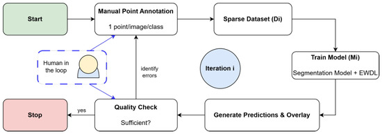
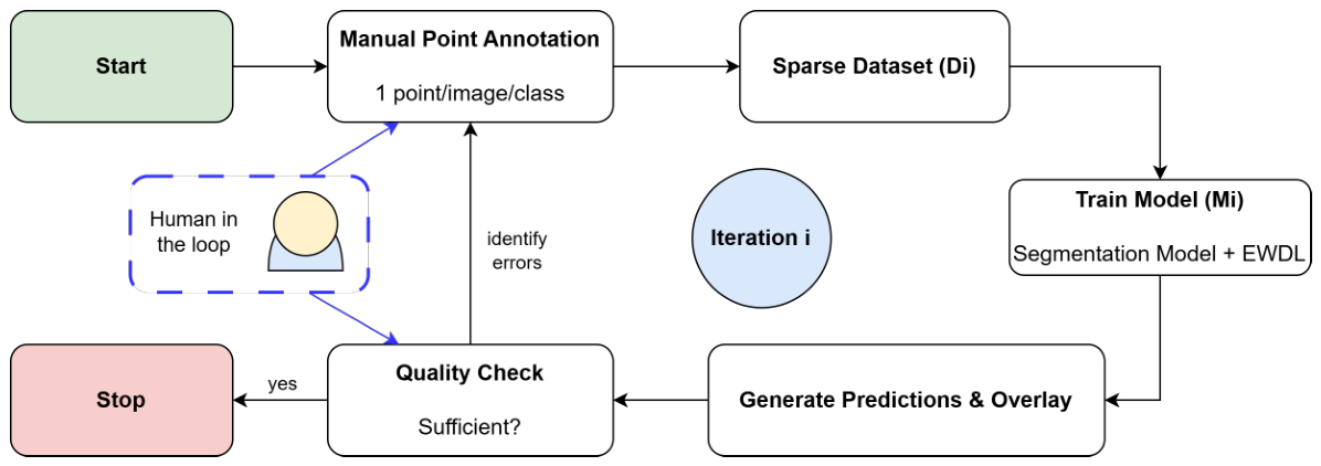
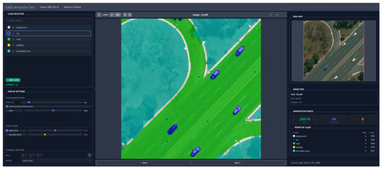
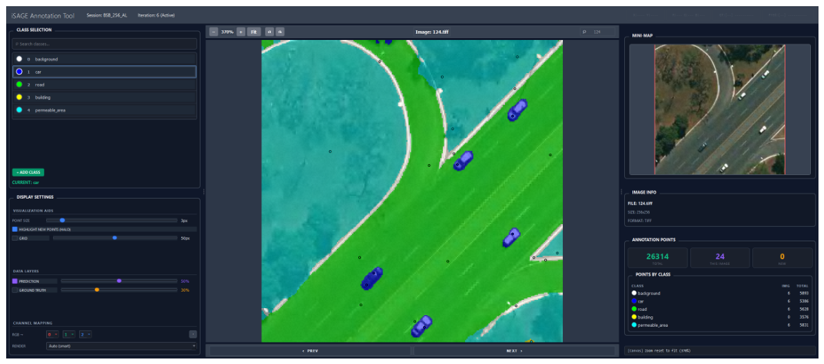
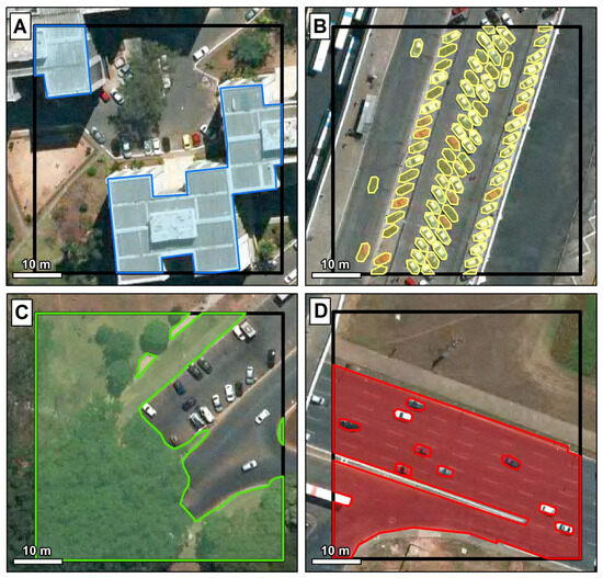
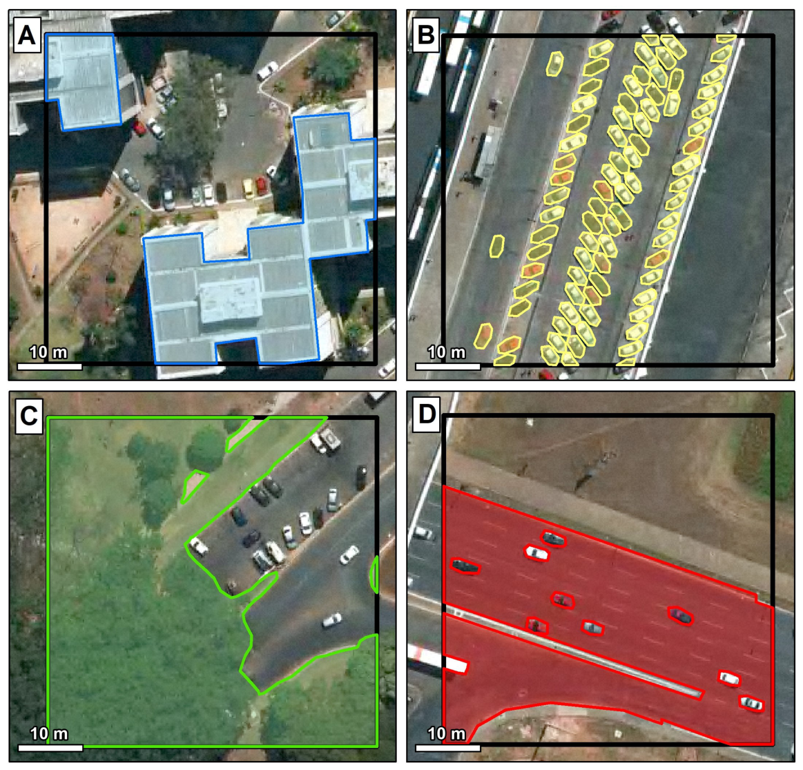
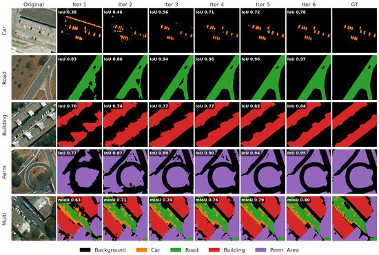
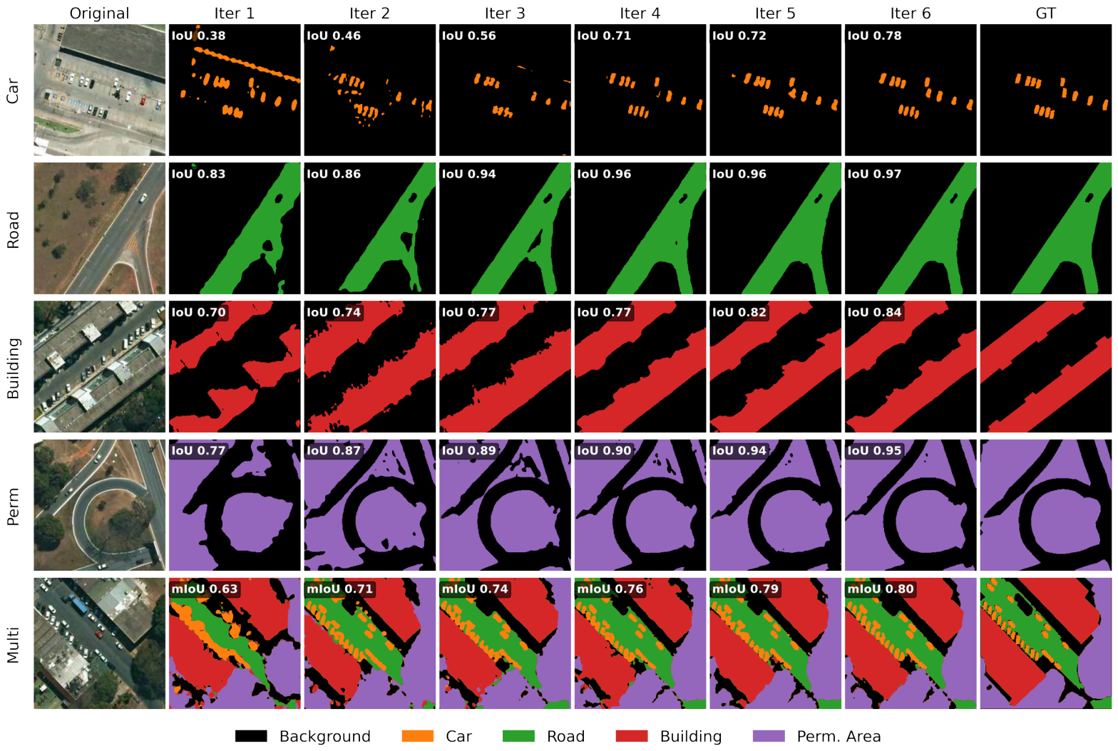
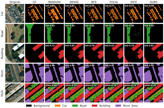
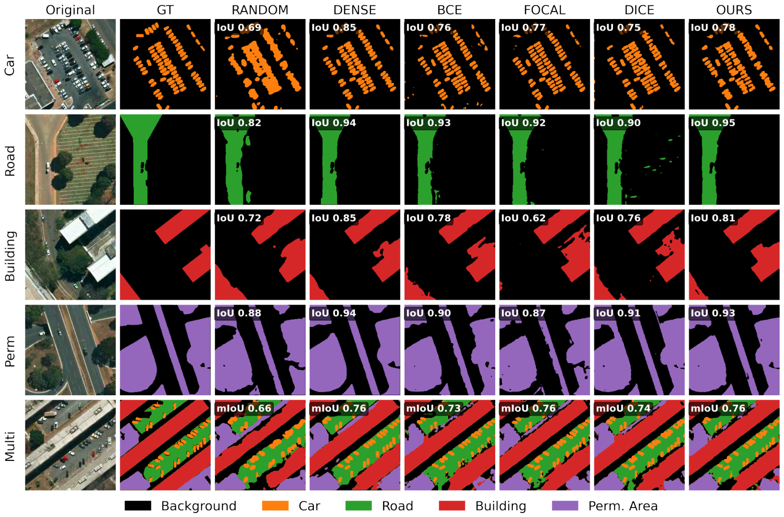
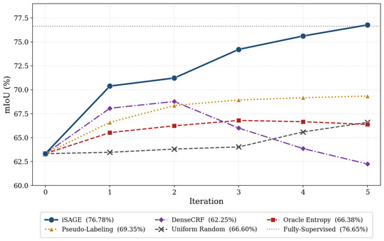
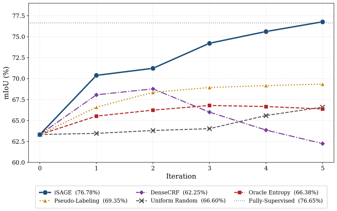
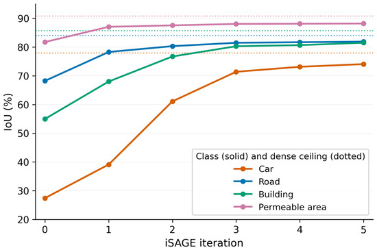
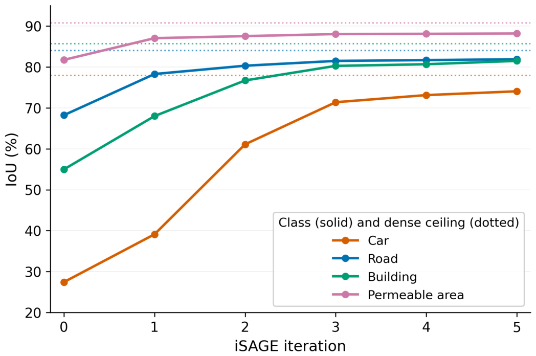

Disclaimer/Publisher’s Note: The statements, opinions and data contained in all publications are solely those of the individual author(s) and contributor(s) and not of MDPI and/or the editor(s). MDPI and/or the editor(s) disclaim responsibility for any injury to people or property resulting from any ideas, methods, instructions or products referred to in the content. |
© 2026 by the authors. Licensee MDPI, Basel, Switzerland. This article is an open access article distributed under the terms and conditions of the Creative Commons Attribution (CC BY) license.