Coherent Integration for Cooperative Bistatic Radar with Joint Time-Domain Waveform Agility

Highlights

What are the main findings?

• The coherent integration loss mechanism of a cooperative bistatic radar for ISAR with simultaneous pulse width (PW) and pulse repetition interval (PRI) agility is analyzed in bistatic radar coordinates.
• PW agility introduces pulse compression mismatch and deterministic residual phase in fast time, while PRI agility causes nonuniform slow-time phase sampling, which destroys the phase consistency required for coherent integration.

What are the implications of the main findings?

• A joint PW and PRI agile processing method is developed to recover coherent gain by coupling fast-time waveform mismatch compensation with nonuniform slow-time phase accumulation.
• Multiple scenario simulations verify improved target focusing, multi-target separation, and motion parameter estimation under the proposed coherent integration method for waveform diversity in the time domain.

Abstract

Waveform agility improves anti-reconnaissance and anti-jamming capability in diverse inverse synthetic aperture radar (ISAR) scenarios, but it also breaks the phase variation assumptions used for conventional coherent processing. For cooperative bistatic ISAR radars, the problem is further complicated by the bistatic geometry and phase evolution induced by synchronization. This paper develops a joint coherent integration method for a cooperative bistatic radar with simultaneous pulse width (PW) and pulse repetition interval (PRI) agility. Firstly, we establish and analyze a bistatic geometric model to reveal key integration problems under agile waveforms, and then derive the coherent processing interval (CPI) local polynomial description for bistatic delay, Doppler and acceleration. On this basis, the matched filter response of each agile pulse is analyzed under the fixed-bandwidth assumption with linear frequency modulation (LFM), showing that PW agility produces a compressed peak displacement and an additional deterministic phase term, whereas PRI agility converts slow-time coherent integration into a nonuniformly sampled spectral estimation problem. To solve this problem, a joint fast and slow-time compensation route is derived, together with a bistatic-specific parameter design method that connects coherent integration tolerances with the bistatic angle and the observable projection vector. Finally, we test the performance of the proposed joint integration method in multiple scenarios and verify its effectiveness and robustness, which enhances detection performance and resolution for target localization.

1. Introduction

Inverse synthetic aperture radar (ISAR) forms high-resolution target images by processing echoes over a coherent processing interval (CPI). In the range Doppler view, wideband pulses provide high range resolution, while the cross-range dimension relies on target-induced aperture and phase continuity across consecutive pulses [1,2]. Bistatic and multistatic ISAR configurations further enrich the observation geometry by separating the transmitter and receiver. Such configurations can provide target information from different aspects and partly relieve the single aspect limitation of monostatic ISAR [3,4,5]. Meanwhile, advances in joint-domain scattering characterization [6] and robust detection with invariant features [7] have demonstrated the value of exploiting richer observation dimensions for radar target analysis. The additional geometry also changes the signal model. The bistatic angle, the equivalent line of sight, and the transmitter–receiver baseline affect envelope alignment, Doppler evolution, and high-order phase terms. Thus, an ISAR-oriented coherent processor for a bistatic system needs a phase model that remains consistent with the actual bistatic observation geometry.

Radar designers often introduce waveform agility to improve survivability and adaptability in complex electromagnetic environments. By varying waveform parameters from pulse to pulse, a radar can reduce the predictability of its emission, improve anti-reconnaissance and anti-jamming capability, and increase waveform diversity [8,9,10,11,12]. In this context, pulse repetition interval ($\mathrm{PRI}$) agility changes the pulse emission times, while pulse width ($\mathrm{PW}$) agility changes the pulse duration and the pulse compression response. Their simultaneous use can provide stronger waveform uncertainty than a single agile parameter, but it also removes the regular pulse-train structure that conventional coherent ISAR processing normally exploits.

Most existing studies treat only part of this dual-agile problem. Researchers have studied random $\mathrm{PRI}$ radar and nonuniform slow-time coherent integration through Radon-type searches, nonuniform fractional Fourier transforms, nonuniform Keystone transforms, and nonuniform fast Fourier transform ($\mathrm{NUFFT}$)-based accumulation [11,13]. Frequency agile radars and radars with random frequency and $\mathrm{PRI}$ agility have also motivated methods that compensate random phase terms associated with carrier frequency or temporal frequency agility [14,15,16]. A smaller number of works consider random $\mathrm{PRI}$ and staggered $\mathrm{PW}$ together, but these treatments are mainly developed for monostatic or general high-speed target detection settings [17]. Recent bistatic $\mathrm{PRI}$-agile coherent integration methods move closer to the present problem by including bistatic geometry and nonuniform pulse timing [18]. Even so, simultaneous $\mathrm{PRI}$ and $\mathrm{PW}$ agility has seen much less systematic treatment in cooperative bistatic coherent processing, especially when pulse timing, pulse duration, and bistatic geometry must be handled in one integration chain.

To clarify the positioning of this work, we compare the proposed method with representative prior approaches. $\mathrm{NUFFT}$-based and Radon methods [11,13,19] mostly handle nonuniform slow-time sampling introduced by random $\mathrm{PRI}$, but they assume a uniform pulse compression response across all pulses and do not model bistatic geometry. For frequency agile radar, existing methods [14,15,16] compensate the phase discontinuities caused by pulse-to-pulse carrier-frequency variations, but they do not address the fast-time envelope mismatch introduced by $\mathrm{PW}$ agility. The monostatic staggered $\mathrm{PW}$ and $\mathrm{PRI}$ method [17] treats both agile parameters simultaneously but formulates the problem in monostatic coordinates and therefore cannot be directly applied to a bistatic baseline. The recent bistatic $\mathrm{PRI}$ agile method [18] incorporates bistatic geometry with nonuniform pulse timing, but it does not account for $\mathrm{PW}$ agility and the associated pulse compression mismatch. In contrast, the present work addresses the case where $\mathrm{PRI}$ agility, $\mathrm{PW}$ agility, and bistatic geometry are all present simultaneously, and it develops a joint fast-time and slow-time compensation framework in bistatic-range coordinates to recover the coherent gain that would otherwise be lost.

These processing routes still carry assumptions that limit their use in the present dual-agile bistatic case. Conventional range-Doppler or pulse-Doppler processing uses a uniform slow-time grid and mutually consistent pulse-compressed echoes, so a matched filter followed by a slow-time FFT is adequate only when the pulse schedule and waveform response remain sufficiently regular. Long-time coherent integration methods such as Keystone transform [20], Radon–Fourier transform, and generalized Radon–Fourier transform compensate range migration and motion-induced phase coupling by searching along hypothesized target trajectories [13,19]. Random-$\mathrm{PRI}$ methods replace the uniform FFT with nonuniform spectral processing, and nonuniform discrete Fourier transform ($\mathrm{NDFT}$)/$\mathrm{NUFFT}$ provides a natural computational tool for such nonuniform samples [11,21]. These methods address important pieces of the problem, but they do not fully describe the fast-time mismatch produced by pulse-to-pulse $\mathrm{PW}$ changes. For a representative fixed-bandwidth linear frequency modulation (LFM) pulse compression waveform [22], changing $\mathrm{PW}$ changes the chirp rate and leads to a pulse-dependent compressed-peak displacement and a deterministic residual phase. Therefore, correcting only the nonuniform slow-time sampling, or only the pulse compression response, leaves a residual mismatch when $\mathrm{PRI}$ and $\mathrm{PW}$ vary simultaneously.

The bistatic configuration adds another modeling constraint. A monostatic formulation usually describes phase history through slant range and radial velocity along a single line of sight. In cooperative bistatic radar, the measured delay is governed by the transmitter–target–receiver bistatic range rather than by a monostatic range. The corresponding Doppler, acceleration, and phase curvature depend on the sum of the transmitter-side and receiver-side line-of-sight projections, and this dependence varies with the bistatic angle [23,24,25,26]. As a result, the Doppler term that enters the pulse compression response is also a bistatic projection, not a monostatic radial component. Directly transplanting a monostatic random-$\mathrm{PRI}$ or staggered-$\mathrm{PW}$ processor therefore does not give the right processing coordinates for a single cooperative bistatic baseline. The coherent integration variables should therefore be placed in the bistatic-range domain, where delay, Doppler, acceleration, and phase curvature remain tied to the observable of the bistatic pair.

Motivated by these issues, this paper studies coherent integration for cooperative bistatic radar with simultaneous $\mathrm{PW}$ and $\mathrm{PRI}$ agility. We formulate the signal model in the bistatic-range domain and use a fixed-bandwidth LFM waveform as a representative pulse-compressed instantiation to make the $\mathrm{PW}$-induced fast-time effect explicit. Based on this model, we combine pulse-wise fast-time shift/phase compensation with nonuniform slow-time phase accumulation on the actual pulse emission times. The same bistatic-range formulation supports ambiguity analysis, parameter-grid design, and controlled simulation tests.

The main contributions are summarized as follows.

• We establish a bistatic-range-domain signal model for cooperative bistatic radar with simultaneous $\mathrm{PW}$ and $\mathrm{PRI}$ agility. Unlike monostatic formulations that describe phase history through slant range and radial velocity along a single line of sight, the proposed model describes delay, Doppler, and higher-order phase terms through the transmitter–target–receiver bistatic range and the bistatic projection vector.
• We characterize the effects of simultaneous $\mathrm{PW}$ and $\mathrm{PRI}$ agility on coherent integration in a unified processing view. Existing $\mathrm{PRI}$-agile methods [11,18] address nonuniform slow-time sampling but assume uniform pulse compression; the present analysis additionally reveals the $\mathrm{PW}$-induced fast-time effect through the fixed-bandwidth LFM instantiation considered here, showing that $\mathrm{PRI}$ agility leads to nonuniform slow-time sampling while $\mathrm{PW}$ agility produces pulse-dependent compression displacement and deterministic residual phase.
• We develop a joint coherent integration method that combines pulse-wise fast-time compensation with nonuniform slow-time phase accumulation on the actual pulse times. This joint processing chain is new: prior bistatic methods [18] compensate only slow-time nonuniformity, and monostatic staggered-$\mathrm{PW}$/$\mathrm{PRI}$ methods [17] do not account for bistatic geometry. We also give bistatic-range-coordinate ambiguity and grid-design rules and validate the method through controlled single-target, two-target, and grid-based estimation experiments.

The rest of the paper is organized as follows. Section 2.1 introduces the cooperative bistatic geometry, waveform schedule, and dual-agile signal model. Section 2.4 develops the joint coherent integration processor. Section 2.5 discusses ambiguity, parameter-grid design, and implementation issues. Section 3 presents the simulation results. Section 5 gives the limitations and conclusions.

This study develops a coherent integration method for cooperative bistatic radar with joint time-domain waveform agility. It uses the bistatic propagation distance and bistatic projection vector to describe the delay, Doppler, acceleration, and higher-order phase terms, and it jointly compensates the fast-time mismatch induced by pulse width agility and the nonuniform slow-time phase history induced by pulse repetition interval agility. This research aims to improve coherent gain recovery, target focusing and dynamic parameter estimation and focuses on four objectives: (1) construct a cooperative bistatic signal model for simultaneous PW and PRI agility, (2) characterize the pulse compression displacement, deterministic residual phase, and nonuniform slow-time sampling effects caused by time domain waveform agility, (3) design a joint fast-time and slow-time coherent integration processor with bistatic specific ambiguity, and (4) verify the effectiveness of the proposed method through numerical simulations.

2. Materials and Methods

2.1. Cooperative Bistatic Geometry

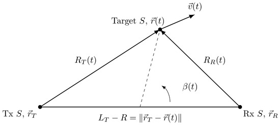
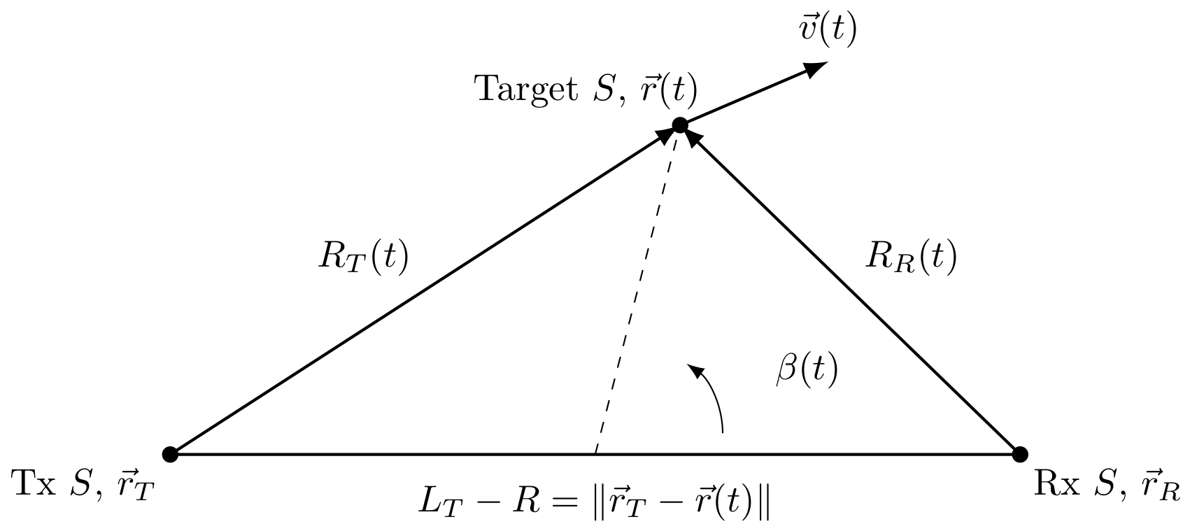
This subsection defines the geometric observable used in the sequel. In a monostatic radar, the propagation variable is usually expressed by a single slant range. In a cooperative bistatic radar, the received echo travels over two propagation legs, from the transmitter to the target and then from the target to the receiver. The corresponding observable is therefore the bistatic range, i.e., the transmitter–target–receiver propagation distance, as shown in Figure 1.

Figure 1. Cooperative bistatic geometry. The fundamental observable is the bistatic range $\rho \left(t\right)=R_T\left(t\right)+R_R\left(t\right)$, namely the transmitter–target–receiver propagation distance.

Consider a cooperative bistatic radar with a transmitter at ${\mathit{r}}_T\in {\mathbb{R}}^3$ and a receiver at ${\mathit{r}}_R\in {\mathbb{R}}^3$. During one coherent processing interval (CPI), the transmitter and receiver are assumed stationary. Under the stop-and-go assumption, the target position is locally represented by

$$\mathit{r}\left(t\right)={\mathit{r}}_0+{\mathit{v}}_{0}t+{\displaystyle \frac{1}{2}}{\mathit{a}}_0{t}^2+{\displaystyle \frac{1}{6}}{\mathit{j}}_0{t}^3,$$

(1)

where $t=0$ is the CPI reference time. This third-order Cartesian expression is used only to introduce the geometry; the coherent processor developed later is formulated in bistatic-range coordinates.

The transmitter–target and target–receiver one-way ranges are

$$R_T\left(t\right)=∥\mathit{r}\left(t\right)-{\mathit{r}}_T∥,R_R\left(t\right)=∥\mathit{r}\left(t\right)-{\mathit{r}}_R∥.$$

(2)

The bistatic range is then

$$\rho \left(t\right)=R_T\left(t\right)+R_R\left(t\right),$$

(3)

and the corresponding propagation delay is

$$\tau \left(t\right)={\displaystyle \frac{\rho \left(t\right)}{c}},$$

(4)

where c is the speed of light. Equation (3) is the key distinction from a monostatic model: the measured delay is determined by the total bistatic propagation distance, not by a single line-of-sight slant range.

Let

$${\widehat{\mathit{u}}}_T\left(t\right)={\displaystyle \frac{\mathit{r}\left(t\right)-{\mathit{r}}_T}{R_T\left(t\right)}},{\widehat{\mathit{u}}}_R\left(t\right)={\displaystyle \frac{\mathit{r}\left(t\right)-{\mathit{r}}_R}{R_R\left(t\right)}}$$

(5)

be the transmitter-side and receiver-side unit line-of-sight vectors. Their sum defines the bistatic projection vector

$$\mathit{b}\left(t\right)={\widehat{\mathit{u}}}_T\left(t\right)+{\widehat{\mathit{u}}}_R\left(t\right),∥\mathit{b}\left(t\right)∥=2cos\left({\displaystyle \frac{\beta \left(t\right)}{2}}\right),$$

(6)

where $\beta \left(t\right)$ is the bistatic angle. This vector describes the component of target motion visible to the bistatic baseline. A motion component that is weakly projected onto $\mathit{b}\left(t\right)$ produces a weak bistatic range rate and hence a weak Doppler contribution.

Differentiating the bistatic range gives

$$\dot{\rho }\left(t\right)={\mathit{b}}^{\mathsf{T}}\left(t\right)\mathit{v}\left(t\right),$$

(7)

where $\mathit{v}\left(t\right)=\dot{\mathit{r}}\left(t\right)$. With approaching motion defined as positive Doppler, the bistatic range rate and bistatic Doppler are

$$v_b\left(t\right)=-\dot{\rho }\left(t\right),f_b\left(t\right)={\displaystyle \frac{v_b\left(t\right)}{\lambda }}=-{\displaystyle \frac{\dot{\rho }\left(t\right)}{\lambda }},$$

(8)

where $\lambda$ is the carrier wavelength. Thus, the Doppler in the following signal model is a bistatic projection of the target motion rather than a monostatic radial component.

Higher-order phase terms have the same geometric nature. The second derivative of $\rho \left(t\right)$ contains both the projection of Cartesian acceleration and the curvature of the two viewing directions. A compact form is

$$\ddot{\rho }\left(t\right)={\dot{\mathit{b}}}^{\mathsf{T}}\left(t\right)\mathit{v}\left(t\right)+{\mathit{b}}^{\mathsf{T}}\left(t\right)\mathit{a}\left(t\right).$$

(9)

This expression is intentionally kept in compact form because the detailed expansion is not needed for the proposed processor. It shows that the apparent bistatic acceleration is not simply the Cartesian acceleration projected onto a fixed direction. Even with constant Cartesian velocity, the changing bistatic viewing geometry can introduce phase curvature.

2.2. CPI-Local Polynomial Parameterization

The coherent integration processor requires an accurate local description of the bistatic phase history over one CPI. It does not require a unique three-dimensional Cartesian state, which cannot be obtained from a single bistatic baseline without additional information. Therefore, the bistatic range is approximated directly by a local polynomial:

$$\rho \left(t\right)\approx {\rho }_0-v_{b0}t-{\displaystyle \frac{1}{2}}{a}_{b0}{t}^2-{\displaystyle \frac{1}{6}}{j}_{b0}{t}^3,$$

(10)

where

$${\rho }_0=\rho \left(0\right),v_{b0}=-\dot{\rho }\left(0\right),a_{b0}=-\ddot{\rho }\left(0\right),j_{b0}=-{\rho }^{\left(3\right)}\left(0\right).$$

(11)

These parameters are bistatic-range-domain motion parameters. They describe the observable delay, Doppler, and phase curvature for the considered transmitter–receiver pair. The main notation used in this paper is summarized in Table 1.

Table 1. Main notation used in the proposed dual-agile bistatic formulation.

Symbol	Meaning	Remark
${\mathit{r}}_T,{\mathit{r}}_R$	transmitter and receiver positions	known during one CPI
$\rho \left(t\right)$	bistatic range	$\rho \left(t\right)=R_T\left(t\right)+R_R\left(t\right)$
$R_b\left(t\right)$	equivalent bistatic range	$R_b\left(t\right)=\rho \left(t\right)/2$ for display
$\tau \left(t\right)$	propagation delay	$\tau \left(t\right)=\rho \left(t\right)/c$
$v_b\left(t\right)$	bistatic range rate	$v_b\left(t\right)=-\dot{\rho }\left(t\right)$
$f_b\left(t\right)$	bistatic Doppler	$f_b\left(t\right)=v_b\left(t\right)/\lambda$
$T_{\mathrm{PW},p}$	width of the pth pulse	agile from pulse to pulse
$T_{\mathrm{PRI},p}$	$\mathrm{PRI}$ preceding the pth pulse	defines the slow-time grid
${\mu }_p$	chirp rate of the pth pulse	${\mu }_p=B/T_{\mathrm{PW},p}$ for fixed bandwidth
$t_p$	emission time of the pth pulse	generally nonuniform
$\theta$	search hypothesis vector	${[{\rho }_0,v_b,a_b,j_b]}^{\mathsf{T}}$

Substituting (10) into the definitions of delay and Doppler gives

$$\tau \left(t\right)\approx {\displaystyle \frac{1}{c}}\left({\rho }_0-v_{b0}t-{\displaystyle \frac{1}{2}}{a}_{b0}{t}^2-{\displaystyle \frac{1}{6}}{j}_{b0}{t}^3\right),$$

(12)

$$f_b\left(t\right)\approx {\displaystyle \frac{1}{\lambda }}\left(v_{b0}+a_{b0}t+{\displaystyle \frac{1}{2}}{j}_{b0}{t}^2\right).$$

(13)

Equations (10)–(13) provide the coordinates used for parameter search. This choice keeps the processing variables consistent with the actual bistatic observable and avoids importing a monostatic slant-range/radial-velocity model.

2.3. Dual-Agile Waveform Schedule and Calibrated Echo Model

Assume that one CPI contains P pulses. The center emission time of the pth pulse is

$$t_p={\displaystyle \sum _{i=0}^{p-1}}{T}_{\mathrm{PRI},i},t_0=0.$$

(14)

If the $\mathrm{PRI}$ varies from pulse to pulse, the slow-time samples ${t_p}_{p=0}^{P-1}$ are nonuniform. This is why the later coherent accumulation must be performed on the actual pulse times rather than on a uniform reference grid.

The transmitted baseband LFM signal for the pth pulse is modeled by

$$s_p(\widehat{t})=rect\left({\displaystyle \frac{\widehat{t}}{T_{\mathrm{PW},p}}}\right)exp\left(\mathrm{j}\pi {\mu }_p{\widehat{t}}^2\right),{\mu }_p={\displaystyle \frac{B}{T_{\mathrm{PW},p}}},$$

(15)

where $\widehat{t}$ denotes fast time within the pulse and B is the fixed transmitted bandwidth. Under the fixed-bandwidth condition, $\mathrm{PW}$ agility changes the chirp rate but does not change the nominal range resolution, which is determined by B.

Before coherent processing, the cooperative receiver is assumed to calibrate the residual transmitter–receiver timing, frequency, and phase offsets using a direct-path signal or an auxiliary reference link. After this calibration, and under the adopted narrowband and stop-and-go assumptions, the baseband echo of the pth pulse is written as

$$r_p(\widehat{t})={\eta }_{p}exp\left(-\mathrm{j}{\displaystyle \frac{2\pi }{\lambda }}\rho (t_p)\right)s_p\left(\widehat{t}-{\tau }_p\right)exp\left(\mathrm{j}2\pi f_{b,p}\widehat{t}\right)+n_p(\widehat{t}),$$

(16)

where

$${\tau }_p={\displaystyle \frac{\rho \left(t_p\right)}{c}},f_{b,p}=f_b\left(t_p\right).$$

(17)

Here, ${\eta }_p$ is the pulse-wise complex scattering coefficient and $n_p(\widehat{t})$ is additive noise. The model retains the effects relevant to this work: bistatic geometric phase, bistatic Doppler, pulse-dependent chirp rate, and nonuniform pulse timing. Residual synchronization errors after cooperative calibration, clutter, and hardware distortion are not explicitly modeled in the theoretical derivation.

The two agile waveform parameters affect different dimensions of the data. $\mathrm{PRI}$ agility changes the slow-time sampling locations, whereas $\mathrm{PW}$ agility changes the pulse compression response through the pulse-dependent chirp rate. This subsection makes these effects explicit.

The matched-filter output for the pth pulse, using the pulse-specific replica, is

$$y_p(\widehat{t})=\int r_p(u)s_p^{*}(u-\widehat{t})\mathrm{d}u.$$

(18)

Substituting the echo model (16) and the transmitted waveform (15) into (18), ignoring the noise term, and writing $\alpha =\widehat{t}-{\tau }_p$ for the delay mismatch, the integral becomes

$$\begin{array}{cc}\hfill y_p(\widehat{t})& ={\eta }_p{\mathrm{e}}^{-\mathrm{j}{\displaystyle \frac{2\pi }{\lambda }}\rho \left(t_p\right)}\int rect\left({\displaystyle \frac{u-{\tau }_p}{T_{\mathrm{PW},p}}}\right)rect\left({\displaystyle \frac{u-\widehat{t}}{T_{\mathrm{PW},p}}}\right)\hfill \\ \hfill & \times exp\left(\mathrm{j}\pi {\mu }_p\left[{(u-{\tau }_p)}^2-{(u-\widehat{t})}^2\right]\right)exp\left(\mathrm{j}2\pi f_{b,p}u\right)\mathrm{d}u.\hfill \end{array}$$

(19)

Using the identity ${(u-{\tau }_p)}^2-{(u-\widehat{t})}^2=(\widehat{t}-{\tau }_p)(2u-\widehat{t}-{\tau }_p)$, the quadratic-phase factor reduces to a linear chirp in u:

$$y_p(\widehat{t})={\eta }_p{\mathrm{e}}^{-\mathrm{j}{\displaystyle \frac{2\pi }{\lambda }}\rho \left(t_p\right)}{\mathrm{e}}^{-\mathrm{j}\pi {\mu }_p\alpha (\widehat{t}+{\tau }_p)}{\int }_{I_p}exp\left(\mathrm{j}2\pi \left[{\mu }_p\alpha +f_{b,p}\right]u\right)\mathrm{d}u,$$

(20)

where $I_p$ is the overlap interval of the two rect windows. When the delay mismatch $\alpha$ is small relative to $T_{\mathrm{PW},p}$, the overlap length is approximately $T_{\mathrm{PW},p}$ and the integral evaluates to

$$y_p(\widehat{t})\approx {\eta }_p{T}_{\mathrm{PW},p}sinc\left(T_{\mathrm{PW},p}[{\mu }_p\alpha +f_{b,p}]\right){\mathrm{e}}^{-\mathrm{j}{\displaystyle \frac{2\pi }{\lambda }}\rho \left(t_p\right)}{\mathrm{e}}^{\mathrm{j}\pi ({\mu }_p\alpha +2f_{b,p})(\widehat{t}+{\tau }_p)/2}{\mathrm{e}}^{-\mathrm{j}\pi {\mu }_p\alpha (\widehat{t}+{\tau }_p)}.$$

(21)

Noting that $T_{\mathrm{PW},p}{\mu }_p=B$ and keeping only the terms that vary with $\widehat{t}$ or p in the phase (terms that are constant across all pulses and delay values do not affect focusing), this simplifies to

$$\begin{array}{cc}\hfill y_p(\widehat{t})& \approx {\eta }_p{T}_{\mathrm{PW},p}sinc\left(B\left[\widehat{t}-{\tau }_p+{\displaystyle \frac{f_{b,p}}{{\mu }_p}}\right]\right)exp\left(-\mathrm{j}{\displaystyle \frac{2\pi }{\lambda }}\rho \left(t_p\right)\right)\hfill \\ \hfill & \times exp\left(\mathrm{j}2\pi f_{b,p}{\tau }_p-\mathrm{j}\pi {\displaystyle \frac{f_{b,p}^2}{{\mu }_p}}\right),\hfill \end{array}$$

(22)

where terms that are constant for the following focusing operation are omitted. The sinc argument is $B[\widehat{t}-{\tau }_p+f_{b,p}/{\mu }_p]$ because the Doppler-induced linear-phase term $f_{b,p}$ shifts the effective center of the LFM cross-correlation by $-f_{b,p}/{\mu }_p$ in fast time; this coupling between Doppler and chirp rate is the mechanism through which $\mathrm{PW}$ agility affects pulse compression. The neglected terms include: (i) the triangular taper of the overlap window, whose effect is less than $0.1$ dB for $\left|\alpha \right|\ll T_{\mathrm{PW},p}$; (ii) the range sidelobes outside the mainlobe; and (iii) the residual Doppler-induced spectral broadening, which satisfies $f_{b,p}{T}_{\mathrm{PW},p}\ll B{T}_{\mathrm{PW},p}$ under the narrowband assumption and is therefore negligible. This expression separates the range-compression envelope from the deterministic phase terms.

First, the envelope mainlobe width remains on the order of $1/B$. Therefore, with fixed bandwidth, $\mathrm{PW}$ agility does not change the nominal range resolution. Second, the compressed peak is shifted to

$${\widehat{t}}_{\mathrm{pk},p}={\tau }_p-{\displaystyle \frac{f_{b,p}}{{\mu }_p}}={\tau }_p-{\displaystyle \frac{f_{b,p}{T}_{\mathrm{PW},p}}{B}}.$$

(23)

Equation (23) follows directly from setting the sinc argument in (22) to zero: $B[\widehat{t}-{\tau }_p+f_{b,p}/{\mu }_p]=0$ gives $\widehat{t}={\tau }_p-f_{b,p}/{\mu }_p$. Physically, because the LFM chirp maps frequency to time, a Doppler shift $f_{b,p}$ displaces the compressed peak by $-f_{b,p}/{\mu }_p$ in fast time. The induced fast-time displacement is

$$\delta {\tau }_{\mathrm{PW},p}=-{\displaystyle \frac{f_{b,p}}{{\mu }_p}}.$$

(24)

This term is pulse-dependent because ${\mu }_p$ changes with $\mathrm{PW}$. Thus, the same bistatic Doppler produces different Doppler-induced range shifts for different pulses.

Third, after the compressed peaks are aligned, a deterministic phase term remains:

$${\varphi }_{\mathrm{PW},p}=2\pi f_{b,p}{\tau }_p-\pi {\displaystyle \frac{f_{b,p}^2}{{\mu }_p}}.$$

(25)

This expression is obtained by evaluating the phase of (22) at the peak location $\widehat{t}={\widehat{t}}_{\mathrm{pk},p}$. The first term $2\pi f_{b,p}{\tau }_p$ arises from the Doppler–delay coupling, and the second term $-\pi f_{b,p}^2/{\mu }_p$ is the quadratic Doppler phase introduced by the chirp-rate-dependent LFM cross-correlation. Because ${\mu }_p=B/T_{\mathrm{PW},p}$, this second term varies from pulse to pulse under $\mathrm{PW}$ agility. The second term in (25) depends explicitly on the chirp rate. It is therefore pulse-dependent under $\mathrm{PW}$ agility and must be compensated before slow-time coherent summation.

Both the displacement and the residual phase are governed by the bistatic Doppler

$$f_{b,p}=-{\displaystyle \frac{1}{\lambda }}{\mathit{b}}^{\mathsf{T}}\left(t_p\right)\mathit{v}\left(t_p\right).$$

(26)

Consequently, the $\mathrm{PW}$-induced fast-time mismatch is controlled by the bistatic projection vector, not by a monostatic radial velocity. This observation naturally leads to a joint compensation strategy: each pulse requires a fast-time shift and phase correction matched to its own chirp rate and predicted bistatic Doppler, and the corrected samples must then be accumulated on the nonuniform slow-time grid caused by $\mathrm{PRI}$ agility.

To verify that the sinc approximation in (22) remains valid under the large $\mathrm{PW}$ span used in the simulations, we compared the approximate output against numerically integrated exact matched-filter results for $\mathrm{PW}$ jitter spans from $0\%$ to $\pm 50\%$. At the simulation setting of $\pm 35\%$, the worst-case peak-shift error is less than $0.001$ $\mathrm{m}$ (compared with the range resolution of $7.5$ $\mathrm{m}$), the residual-phase error is less than 1.4° (compared with the $\pi /4$ coherent-phase tolerance), and the amplitude error is below $0.01\%$. These errors remain negligible across the entire jitter range because the approximation quality is governed by $|f_{b,p}|/B\approx 0.003\ll 1$, a ratio that is independent of the pulse width. Therefore, the sinc-form approximation is well justified for the parameter regime of this study.

2.4. Proposed Joint Fast-Time and Slow-Time Coherent Integration Method

The processor searches directly in bistatic-range coordinates. This choice is consistent with a single cooperative bistatic baseline, whose directly observable quantities are delay, Doppler, and phase curvature associated with $\rho \left(t\right)$ rather than a unique Cartesian target state.

A search hypothesis is defined as

$$\theta ={[{\rho }_{0,s},v_{b,s},a_{b,s},j_{b,s}]}^{\mathsf{T}}.$$

(27)

It induces the predicted bistatic range

$${\rho }_s\left(t\right)={\rho }_{0,s}-v_{b,s}t-{\displaystyle \frac{1}{2}}{a}_{b,s}{t}^2-{\displaystyle \frac{1}{6}}{j}_{b,s}{t}^3,$$

(28)

and hence the predicted delay and Doppler at the actual pulse time $t_p$:

$${\tau }_{s,p}={\displaystyle \frac{{\rho }_s\left(t_p\right)}{c}},f_{s,p}={\displaystyle \frac{1}{\lambda }}\left(v_{b,s}+a_{b,s}{t}_p+{\displaystyle \frac{1}{2}}{j}_{b,s}{t}_p^2\right).$$

(29)

These predicted quantities determine both the fast-time correction and the slow-time phase compensation. A correct hypothesis simultaneously aligns the compressed-pulse envelopes and flattens the bistatic geometric phase over the CPI.

Fast-time compensation is designed to remove the $\mathrm{PW}$-induced compressed-peak displacement and the deterministic chirp-rate-dependent phase. For each hypothesis, the processor predicts ${\tau }_{s,p}$ and $f_{s,p}$ for every pulse and then applies a pulse-wise correction.

The compensated pulse compression output is defined as

$$z_p(\widehat{t};\theta )=y_p\left(\widehat{t}-{\displaystyle \frac{f_{s,p}}{{\mu }_p}}\right)exp\left[-\mathrm{j}2\pi f_{s,p}{\tau }_{s,p}+\mathrm{j}\pi {\displaystyle \frac{f_{s,p}^2}{{\mu }_p}}\right].$$

(30)

The sign convention in (30) is chosen to undo the effects identified in (23)–(25). The argument shift subtracts $f_{s,p}/{\mu }_p$, which counteracts the Doppler-induced peak displacement $-f_{b,p}/{\mu }_p$ in (24): under the correct hypothesis ($f_{s,p}=f_{b,p}$), evaluating $z_p$ at $\widehat{t}={\tau }_{s,p}={\tau }_p$ yields $y_p({\tau }_p-f_{b,p}/{\mu }_p)=y_p\left({\widehat{t}}_{\mathrm{pk},p}\right)$, which is the peak of the matched-filter output. The exponential factor $exp[-\mathrm{j}2\pi f_{s,p}{\tau }_{s,p}+\mathrm{j}\pi f_{s,p}^2/{\mu }_p]$ is exactly the negative of the residual phase ${\varphi }_{\mathrm{PW},p}$ in (25), so that both the envelope displacement and the deterministic phase are removed simultaneously. The corrected sample is then taken along the predicted delay trajectory:

$$x_p\left(\theta \right)=z_p({\tau }_{s,p};\theta ).$$

(31)

Let the prediction errors be

$$\Delta {\tau }_p={\tau }_{s,p}-{\tau }_p,\Delta f_p=f_{s,p}-f_{b,p}.$$

(32)

Substituting (22) into (30) gives the dominant envelope term

$$x_p\left(\theta \right)\propto sinc\left(B\left[\Delta {\tau }_p-{\displaystyle \frac{\Delta f_p}{{\mu }_p}}\right]\right)exp\left(-\mathrm{j}{\displaystyle \frac{2\pi }{\lambda }}\rho \left(t_p\right)\right)exp\left(\mathrm{j}{\varphi }_p^{\mathrm{res}}\right),$$

(33)

where ${\varphi }_p^{\mathrm{res}}$ is the remaining deterministic phase error. Under the correct hypothesis, the envelope mismatch and the residual deterministic phase vanish up to noise and scattering fluctuations.

Equation (33) gives the fast-time focusing condition

$$\left|\Delta {\tau }_p-{\displaystyle \frac{\Delta f_p}{{\mu }_p}}\right|\ll {\displaystyle \frac{1}{B}}.$$

(34)

This condition shows that delay mismatch and Doppler mismatch are coupled inside the $\mathrm{PW}$-agile LFM mainlobe. Therefore, correcting only the nominal delay is not sufficient when the chirp rate varies and the bistatic Doppler is non-negligible.

After the pulse-wise fast-time correction, the dominant deterministic term is the bistatic geometric phase. For the same hypothesis, this phase is removed as

$${\tilde{x}}_p\left(\theta \right)=x_p\left(\theta \right)exp\left(\mathrm{j}{\displaystyle \frac{2\pi }{\lambda }}{\rho }_s\left(t_p\right)\right).$$

(35)

If the hypothesis is correct, the phase of ${\tilde{x}}_p\left(\theta \right)$ becomes approximately constant over the CPI, apart from noise and scattering fluctuations.

The coherent statistic is

$$\Lambda \left(\theta \right)={\left|{\displaystyle \sum _{p=0}^{P-1}}{w}_p{\tilde{x}}_p\left(\theta \right)\right|}^2,$$

(36)

where $w_p$ is a pulse-weighting factor. Natural weighting $w_p=1$ is used when constant peak transmit power is assumed, because longer pulses produce larger matched-filter output energy. Equalized weighting may be used if amplitude balancing across a large $\mathrm{PW}$ span is desired.

The important point is that the summation in (36) is evaluated at the actual pulse times $\left\{t_p\right\}$. Since $\mathrm{PRI}$ agility makes these times nonuniform, the operation is not a conventional FFT on a uniform slow-time grid. It is a nonuniform spectral estimation problem. For the polynomial model,

$$exp\left(\mathrm{j}{\displaystyle \frac{2\pi }{\lambda }}{\rho }_s\left(t\right)\right)={\mathrm{e}}^{\mathrm{j}2\pi {\rho }_{0,s}/\lambda }{\mathrm{e}}^{-\mathrm{j}2\pi {\nu }_{s}t}{\mathrm{e}}^{-\mathrm{j}2\pi {\kappa }_s{t}^2}{\mathrm{e}}^{-\mathrm{j}2\pi {\xi }_s{t}^3},$$

(37)

with

$${\nu }_s={\displaystyle \frac{v_{b,s}}{\lambda }},{\kappa }_s={\displaystyle \frac{a_{b,s}}{2\lambda }},{\xi }_s={\displaystyle \frac{j_{b,s}}{6\lambda }}.$$

(38)

After the acceleration and jerk terms are compensated or searched, the residual search over ${\nu }_s$ can be implemented by direct $\mathrm{NDFT}$ or by $\mathrm{NUFFT}$-based acceleration on the nonuniform grid [21]. This is an implementation choice rather than a change in the signal model.

The proposed processor has a two-layer structure (Algorithm 1). The first layer performs pulse-wise fast-time shift and phase correction to handle $\mathrm{PW}$ agility. The second layer removes the bistatic geometric phase and coherently accumulates the corrected samples on the actual pulse-time grid caused by $\mathrm{PRI}$ agility.

Algorithm 1 Joint coherent integration for dual-agile cooperative bistatic LFM radar.

Require: Pulse-compressed data ${\left\{y_p\left(\widehat{t}\right)\right\}}_{p=0}^{P-1}$, waveform schedule $\{T_{\mathrm{PW},p},T_{\mathrm{PRI},p}\}$, hypothesis set $\Theta$   1: Generate the actual pulse times $\left\{t_p\right\}$ from the $\mathrm{PRI}$ schedule.   2: for each $\theta ={[{\rho }_{0,s},v_{b,s},a_{b,s},j_{b,s}]}^{\mathsf{T}}\in \Theta$ do   3:       Predict ${\rho }_s\left(t_p\right)$, ${\tau }_{s,p}$, and $f_{s,p}$ for all pulses.   4:       Apply pulse-wise fast-time shift and deterministic phase compensation using (30).   5:       Sample the corrected output at the predicted delay to obtain $x_p\left(\theta \right)$.   6:       Remove the bistatic geometric phase using (35).   7:       Accumulate the corrected sequence on the nonuniform pulse-time grid using (36).   8: end for   9: return  $\widehat{\theta }={arg\; max}_{\theta \in \Theta }\Lambda \left(\theta \right)$

2.5. Ambiguity, Grid Design, and Implementation Discussion

2.5.1. Doppler and Range Ambiguity Under Dual Agility

Ambiguity should be described in the same coordinates as the signal model. In the present problem, delay ambiguity is a bistatic-range ambiguity, and Doppler ambiguity is associated with the bistatic range rate.

For a uniform $\mathrm{PRI}$$T_r$, the classical Doppler ambiguity interval is

$$\Delta f_{b,\mathrm{amb}}={\displaystyle \frac{1}{T_r}},\Delta v_{b,\mathrm{amb}}={\displaystyle \frac{\lambda }{T_r}}.$$

(39)

Under a far-field approximation, the velocity component along the bistatic bisector satisfies

$$f_b\approx {\displaystyle \frac{2cos(\beta /2)}{\lambda }}{v}_{\Vert },$$

(40)

which gives the corresponding physical-velocity ambiguity interval

$$\Delta v_{\Vert ,\mathrm{amb}}\approx {\displaystyle \frac{\lambda }{2T_{r}cos(\beta /2)}}.$$

(41)

Thus, the same Doppler ambiguity maps to different physical-velocity intervals for different bistatic angles.

When the $\mathrm{PRI}$ is agile, ambiguity is governed by the actual pulse times. Two Doppler frequencies separated by $\Delta \nu$ are indistinguishable on the acquired slow-time samples only if

$$exp\left(-\mathrm{j}2\pi \Delta \nu t_p\right)=1,p=0,\dots ,P-1.$$

(42)

This condition explains why a uniform-$\mathrm{PRI}$ FFT ambiguity interval cannot be directly used for agile-$\mathrm{PRI}$ data. If the pulse times lie on a clock lattice $t_p=q_p{T}_c$ with integer $q_p$, a useful special case is

$$\Delta {\nu }_{\mathrm{amb}}={\displaystyle \frac{1}{g{T}_c}},g=gcd(q_0,q_1,\dots ,q_{P-1}).$$

(43)

For a general nonuniform schedule, the ambiguity behavior should be evaluated from the actual sampling pattern and its sidelobe structure.

The range ambiguity is also expressed through the bistatic range. At the pulse level, avoiding overlap requires approximately

$$0\le {\rho }_p<c{T}_{\mathrm{PRI},p}.$$

(44)

If an equivalent bistatic range $R_b=\rho /2$ is used for display, then

$$0\le R_{b,p}<{\displaystyle \frac{c{T}_{\mathrm{PRI},p}}{2}}.$$

(45)

Including the pulse width and a receiver guard interval $T_g$ gives the conservative safe bound

$${\rho }_{\mathrm{safe}}\lesssim c\underset{p}{min}\left(T_{\mathrm{PRI},p}-T_{\mathrm{PW},p}-T_g\right).$$

(46)

Finally, even after delay and Doppler are correctly unwrapped, a single bistatic baseline does not uniquely determine the Cartesian target state. A fixed bistatic range defines an iso-range ellipsoid, and a fixed bistatic Doppler defines an iso-Doppler surface. Their intersection is generally nonunique. The proposed processor therefore estimates bistatic-range-domain motion parameters rather than a fully observable three-dimensional state.

2.5.2. Bistatic-Specific Parameter-Grid Design

The hypothesis grid must be fine enough to preserve both fast-time focusing and slow-time phase coherence. A grid that is too coarse can move the compressed response away from the mainlobe or cause phase decorrelation during coherent accumulation.

Let the hypothesis mismatch be

$$\delta \theta ={[\delta {\rho }_0,\delta v_b,\delta a_b,\delta j_b]}^{\mathsf{T}},$$

(47)

which induces the bistatic-range mismatch

$$\Delta \rho \left(t\right)=\delta {\rho }_0-\delta v_{b}t-{\displaystyle \frac{1}{2}}\delta a_b{t}^2-{\displaystyle \frac{1}{6}}\delta j_b{t}^3.$$

(48)

The corresponding delay and Doppler errors are

$$\Delta \tau \left(t\right)={\displaystyle \frac{\Delta \rho \left(t\right)}{c}},\Delta f\left(t\right)={\displaystyle \frac{1}{\lambda }}\left(\delta v_b+\delta a_{b}t+{\displaystyle \frac{1}{2}}\delta j_b{t}^2\right).$$

(49)

The fast-time focusing tolerance follows from the $\mathrm{PW}$-agile LFM mainlobe:

$$\underset{p}{max}\left|\Delta \tau \left(t_p\right)-{\displaystyle \frac{\Delta f\left(t_p\right)}{{\mu }_p}}\right|\le {\displaystyle \frac{{\eta }_r}{B}},$$

(50)

where $0<{\eta }_r<1$ is a chosen fraction of the range-compression mainlobe. This condition jointly constrains delay error and Doppler-induced peak displacement.

The slow-time phase tolerance gives a second requirement:

$$\underset{p}{max}\left|{\displaystyle \frac{2\pi }{\lambda }}\Delta \rho \left(t_p\right)\right|\le {\eta }_{\varphi },$$

(51)

where ${\eta }_{\varphi }$ is the allowed phase error. In practice, the step size of each parameter should satisfy both (50) and (51).

For example, let $T_{\mathrm{CPI}}={max}_p{t}_p$ and $T_{\mathrm{PW},max}={max}_p{T}_{\mathrm{PW},p}$. Representative conservative bounds for the initial bistatic range and bistatic range rate are

$$|\delta {\rho }_0|<min\left({\eta }_r{\displaystyle \frac{c}{B}},{\displaystyle \frac{{\eta }_{\varphi }\lambda }{2\pi }}\right),$$

(52)

$$|\delta v_b|<min\left[{\displaystyle \frac{{\eta }_r/B}{T_{\mathrm{CPI}}/c+T_{\mathrm{PW},max}/\left(\lambda B\right)}},{\displaystyle \frac{{\eta }_{\varphi }\lambda }{2\pi T_{\mathrm{CPI}}}}\right].$$

(53)

The acceleration and jerk steps are obtained analogously by using the corresponding second- and third-order time factors. These rules are conservative design guidelines, not unique optimal grid choices.

The bistatic angle enters the physical interpretation of these steps through the projection vector. At the CPI reference time,

$${\mathit{b}}_0={\widehat{\mathit{u}}}_T\left(0\right)+{\widehat{\mathit{u}}}_R\left(0\right),∥{\mathit{b}}_0∥=2cos\left({\displaystyle \frac{{\beta }_0}{2}}\right).$$

(54)

For small perturbations,

$$\delta {\rho }_0\approx {\mathit{b}}_0^{\mathsf{T}}\delta {\mathit{r}}_0,\delta v_b\approx -{\mathit{b}}_0^{\mathsf{T}}\delta {\mathit{v}}_0.$$

(55)

Therefore, along the bistatic projection direction,

$$|\delta r_{\Vert }|<{\displaystyle \frac{\Delta {\rho }_0}{2cos({\beta }_0/2)}},\left|\delta v_{\Vert }\right|<{\displaystyle \frac{\Delta v_b}{2cos({\beta }_0/2)}}.$$

(56)

This mapping shows why a monostatic grid rule cannot be directly transplanted to the bistatic case. The physical-space resolution associated with a given bistatic-range-domain step depends on the bistatic projection strength.

2.5.3. Implementation and Computational Remarks

A direct four-dimensional search over $N_{\rho }\times N_v\times N_a\times N_j$ hypotheses has the dominant scaling

$$\mathcal{O}\left(N_{\rho }{N}_v{N}_a{N}_{j}P\right),$$

(57)

excluding implementation interpolation and memory costs. This complexity is acceptable for controlled validation grids, but it can become expensive for fine operational searches.

Several observations follow from the derivation. First, the fast-time compensation in (30) is separable across pulses and hypotheses. The interpolation shifts and phase factors can therefore be parallelized, and repeated terms can be tabulated over coarse values of $({\tau }_s,f_s,{\mu }_p)$. Second, after range, acceleration, and jerk terms are fixed or compensated, the remaining velocity-related search has the structure of nonuniform spectral estimation over $\left\{t_p\right\}$. Direct $\mathrm{NDFT}$ is straightforward, while $\mathrm{NUFFT}$ can reduce the slow-time search cost for large grids [21]. Third, the grid rules in Section 2.5 are also useful for computational pruning because they indicate when further refinement is unlikely to improve focusing under the adopted model.

No claim of real-time implementation is made here. The purpose of this discussion is to identify the main computational bottlenecks and the natural acceleration points implied by the bistatic-range-domain derivation.

To provide a concrete reference, we measured the wall-clock time of the proposed method and representative baselines under the default simulation parameters (Table 2) on a standard desktop platform (MATLAB R2022b, Intel desktop CPU). For a two-dimensional range–velocity search grid of size $81\times 81$ with $P=128$ pulses, the proposed joint compensation method requires approximately $21.8$ $\mathrm{s}$, compared with $21.2$ $\mathrm{s}$ for the Radon-FFT baseline. The per-hypothesis evaluation time is approximately $3.2$ $\mathrm{m}$$\mathrm{s}$ for all methods, indicating that the additional fast-time compensation steps (interpolation shift and phase correction) add less than $5\%$ overhead relative to the baseline that omits them. The computational cost is therefore dominated by the total number of search hypotheses rather than by the compensation complexity of any single evaluation.

Table 2. Principal simulation parameters used in this study.

Parameter	Value
Carrier frequency $f_c$	5 GHz
Bandwidth B	20 MHz
Number of pulses in CPI	128
Range of agile PRI	$\Delta PRI\sim \mathrm{U}(0.45,0.75)$ ms
Range of agile PW	$\Delta PW\sim \mathrm{U}(25,55)$ µs
Sampling rate	40 MHz
Baseline bistatic angle for design study	${\beta }_0$ = 60°
Range grid spacing $\Delta {\rho }_0$	12 m
Velocity grid spacing $\Delta v_b$	10 m s−1
Acceleration grid spacing $\Delta a_b$	2.6 m s−2
Jerk grid spacing $\Delta j_b$	104 m s−3
Number of Monte Carlo trials	50

Several acceleration strategies can significantly reduce the processing time for operational-scale grids: (1) replacing the direct $\mathrm{NDFT}$ with $\mathrm{NUFFT}$ reduces the per-hypothesis slow-time spectral cost from $\mathcal{O}\left(P^2\right)$ to $\mathcal{O}(PlogP)$; (2) the hypothesis evaluations are mutually independent and can be distributed across CPU cores via parallel loops or onto a GPU; (3) a coarse-to-fine two-stage search can first locate candidate peaks on a coarse grid using a computationally lighter method (e.g., Radon-FFT) and then refine each candidate with the full joint compensator on a local fine grid, reducing the total number of full evaluations by one to two orders of magnitude. These strategies are complementary and their combination can bring the runtime well within practical limits for non-real-time applications.

3. Results

3.1. Simulation Setup

In this section, we first carry out simulation experiments to test the proposed integration method for a single target to prove its feasibility. Then we test the integration method for multi-target scenarios to compare its robustness with conventional integration methods. Finally, we analyze and compare the detection performance, and the motion parameter estimation performance.

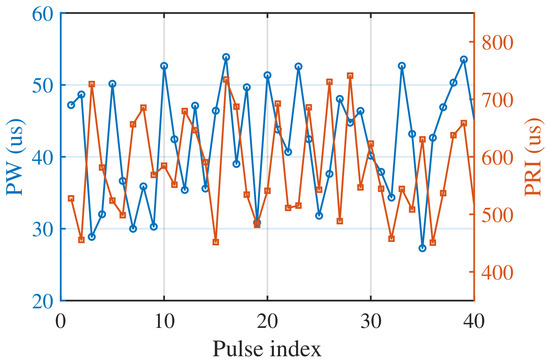
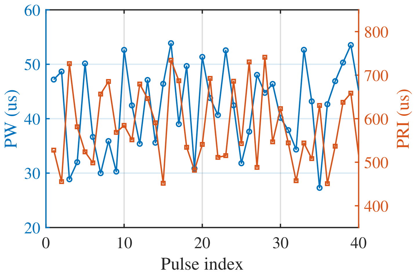
The agile PRI and PW are random variables with a uniform distribution. The parameters of bistatic agile radar simulated in this work are shown in Table 2. A case of waveform agility in the time domain is shown in Figure 2, which illustrates the slow-time consequence of both $\mathrm{PRI}$ agility and PW agility. The actual pulse times depart from a uniform reference grid, and the unwrapped slow-time phase becomes nearly flat only after bistatic geometric compensation. Additionally, unless otherwise noted, the processing CPI uses $P=128$ pulses with $\mathrm{PW}$ jitter span $\pm 35\%$ and $\mathrm{PRI}$ jitter span $\pm 25\%$. For some experiments, the simulation signal-to-noise ratio (SNR) is adjusted to emphasize detection, RMSE, or multi-target features.

Figure 2. Representative dual-agile schedule used in the simulation package. The pulse width and pulse repetition interval both vary from pulse to pulse, so the fast-time-matched filter and the slow-time accumulation kernel cannot be fixed across the $\mathrm{CPI}$.

3.2. Coherent Integration in Single-Target Scenario

The method is first tested on the single-target scenario. The motion parameters of the target are as follows: the initial range is 200 km, corresponding to an equivalent bistatic range of 100 km, with initial velocity and acceleration set as $v_b$ = 3200 m s⁻¹ and $a_b$ = 40 m s⁻², respectively.

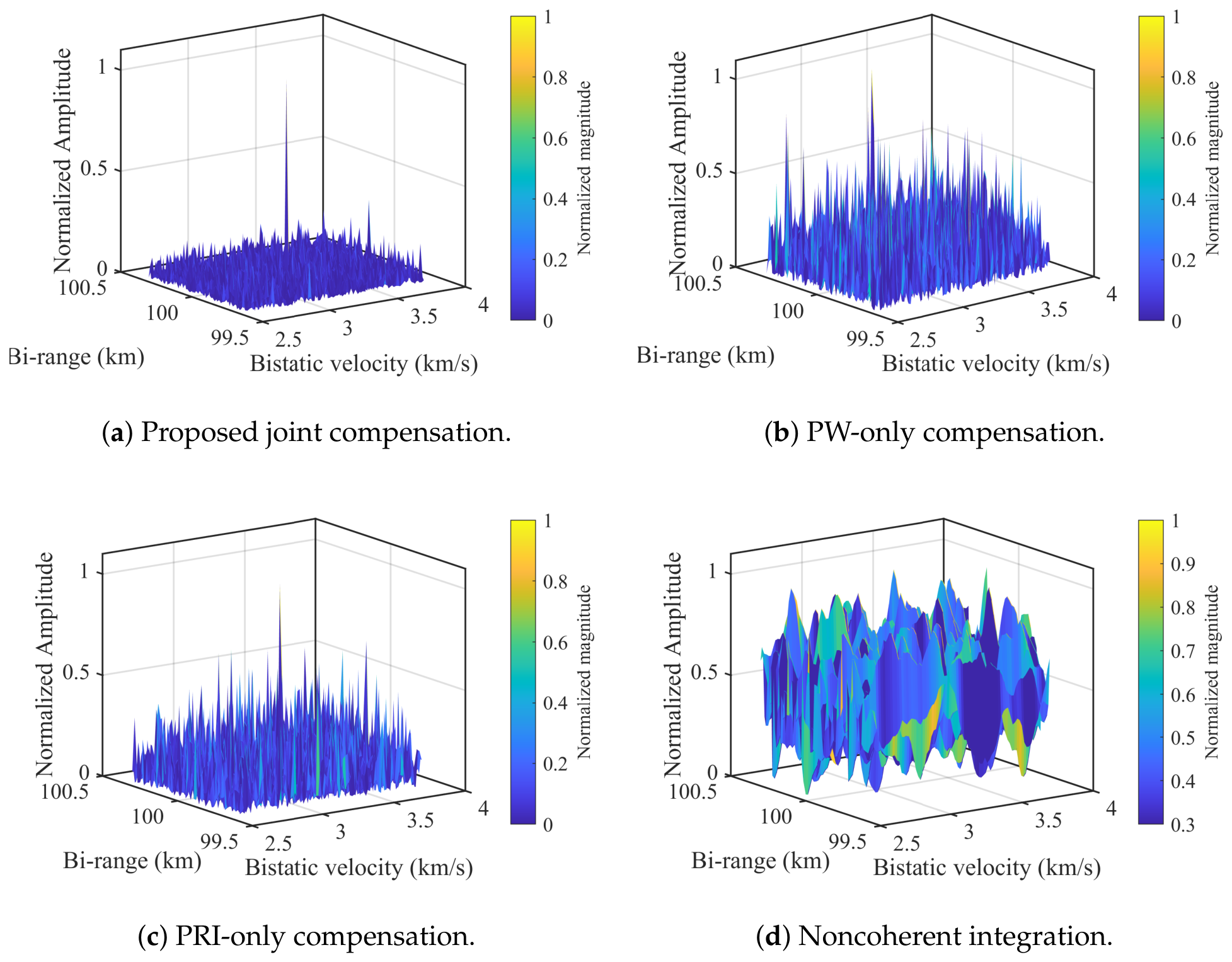
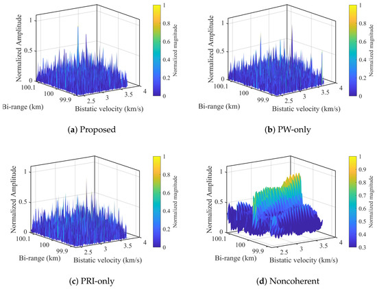
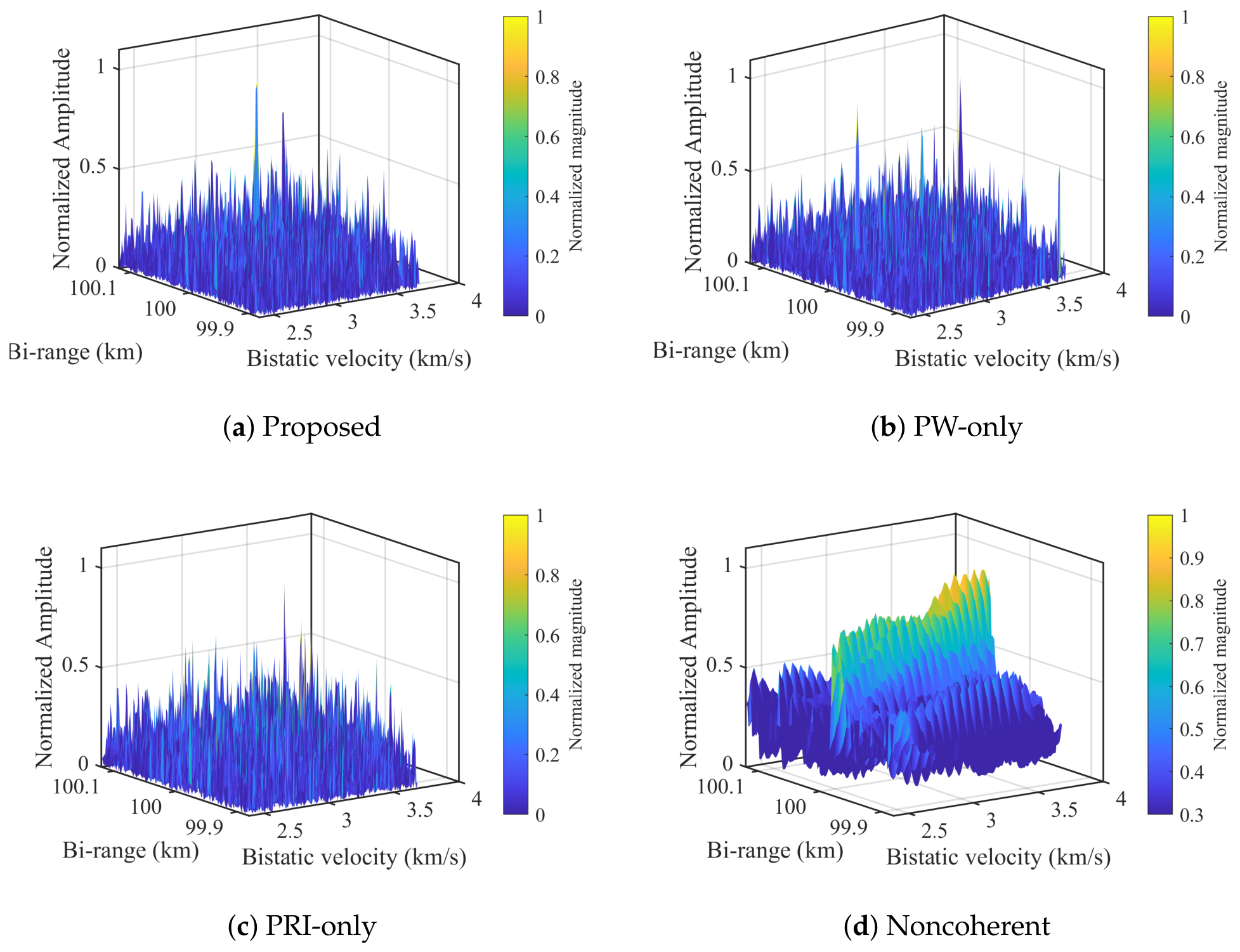
Due to the lack of research on coherent processing of agile bistatic radar, we use an ablation experiment to test the two-step coherent processing method, including the proposed coherent processing method, coherent processing with compensation of PW agility only, coherent processing with compensation of PRI agility only, and noncoherent processing. Specifically, the proposed coherent processing method includes both $\mathrm{PW}$ shift compensation and nonuniform slow-time coherent integration. Coherent processing with compensation of PW agility only (PW-only) concentrates on fast-time $\mathrm{PW}$ compensation only, while slow time is processed using a uniform reference phase history. In contrast, coherent processing with compensation of PRI agility only (PRI-only) focuses on slow-time bistatic geometric compensation without correcting the $\mathrm{PW}$-induced fast-time mismatch. The noncoherent method considers only magnitude integration and is used as a low-complexity reference.

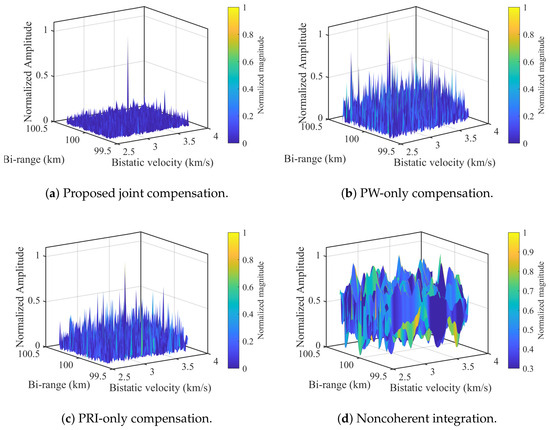
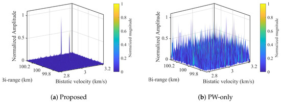
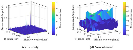
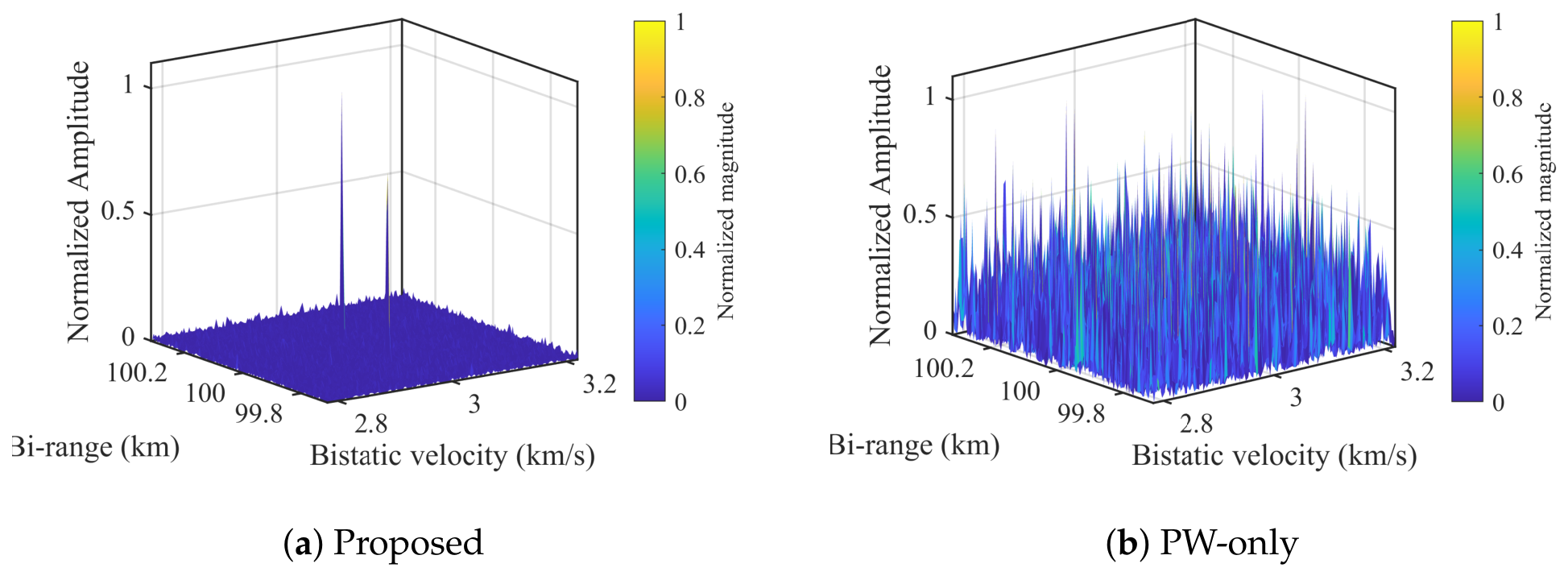
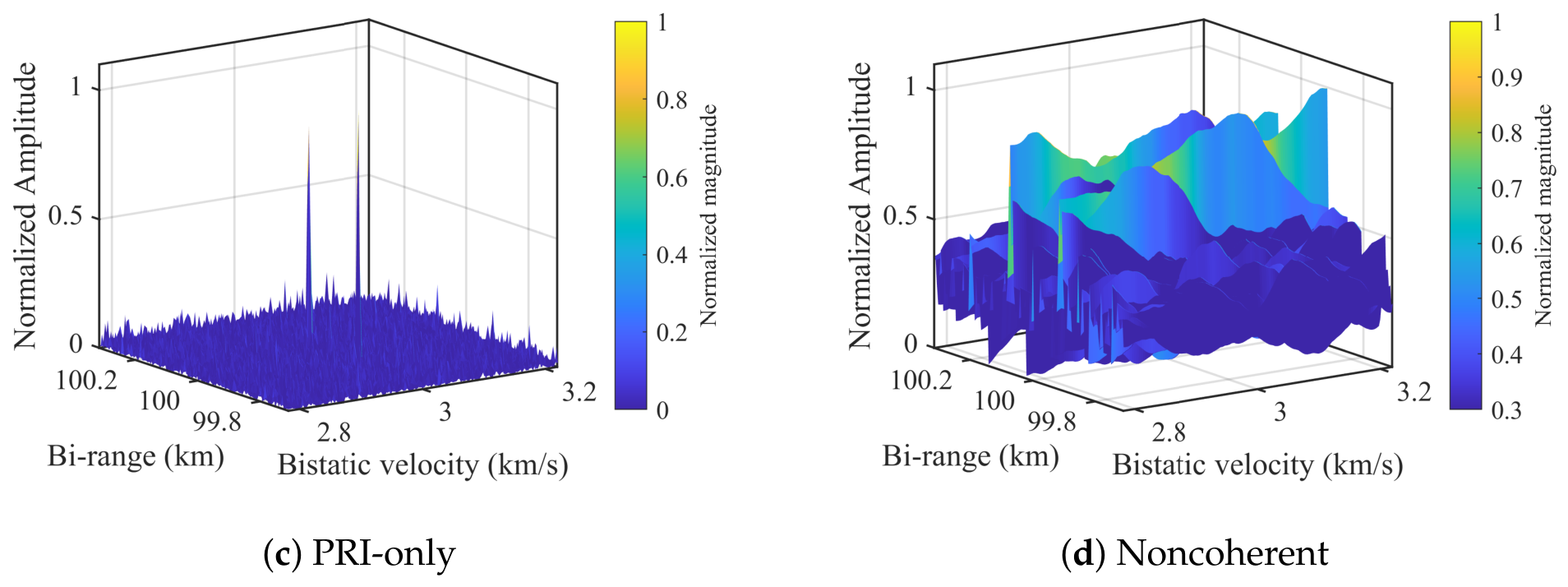
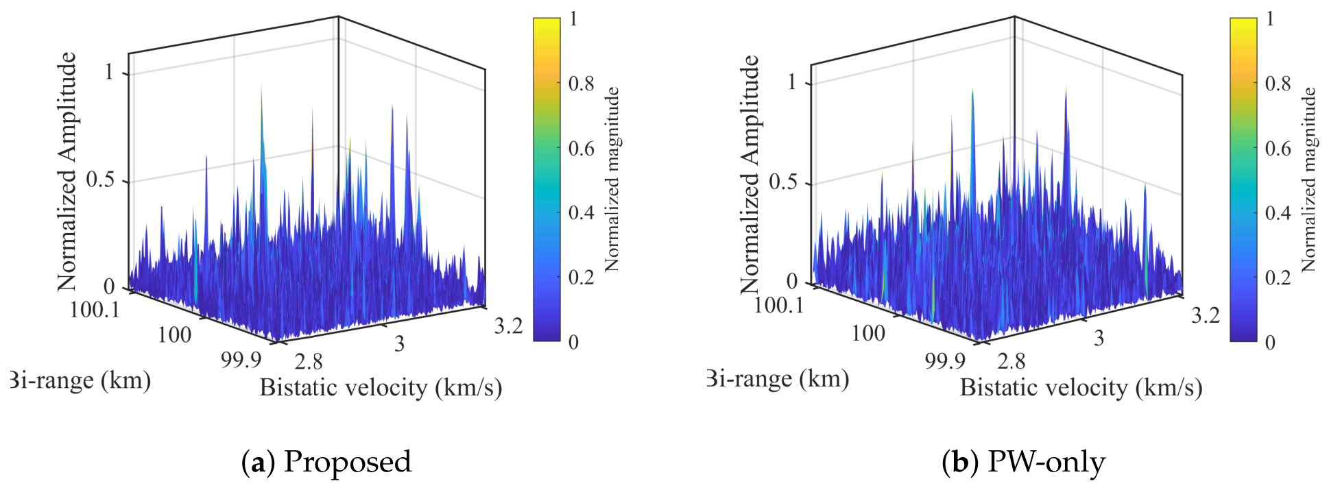
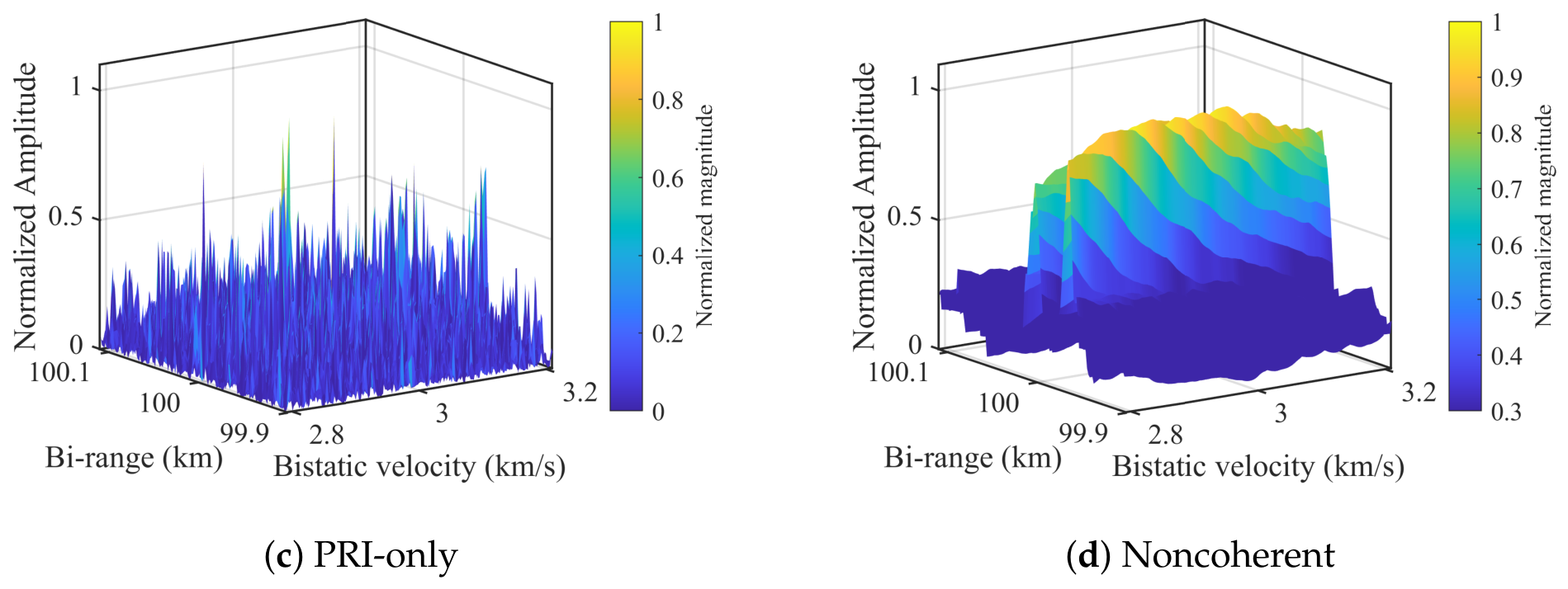
Figure 3 compares the range–velocity maps for a single target under a low-SNR setting. The proposed method produces a single dominant and well-localized peak. In contrast, the $\mathrm{PW}$-only method leaves an elevated and highly irregular floor because the slow-time phase remains mismatched, while the $\mathrm{PRI}$-only method retains a visible focus loss because the fast-time pulse compression peaks are not properly aligned. The noncoherent result is the broadest and least selective, as expected.

Figure 3. Single-target range–velocity maps. The proposed method yields the sharpest and most isolated peak because it compensates both the $\mathrm{PW}$-induced fast-time mismatch and the nonuniform slow-time phase history. Partial-compensation baselines leave substantial residual defocus.

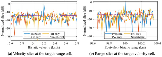
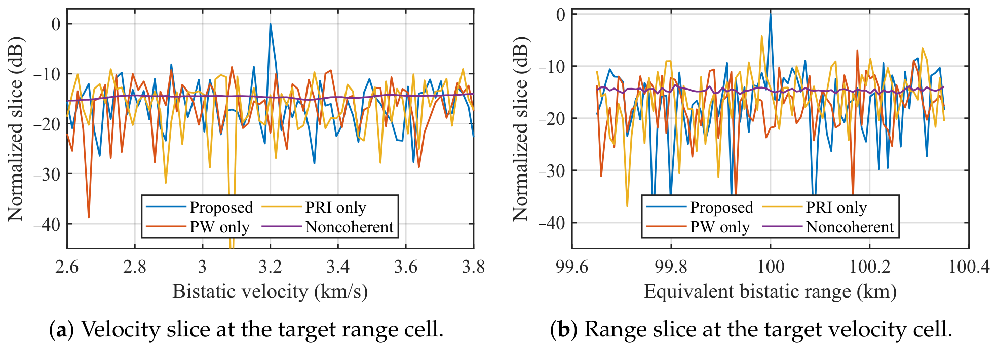
The slice views in Figure 4 support the same conclusion from one-dimensional cuts. At the true range, the proposed method gives the narrowest velocity slice and the highest contrast between the mainlobe and the surrounding floor. At the true velocity, it also produces the cleanest range slice. These slice plots are important because the 3D surfaces of Figure 3 can hide floor differences at low SNR; the one-dimensional cuts make the focusing advantage directly visible.

Figure 4. Single-target slice comparison. The proposed method exhibits the most concentrated mainlobe in both dimensions, whereas incomplete compensation leaves higher sidelobe-like fluctuations and poorer peak contrast.

To quantify the focusing quality beyond visual comparison, Table 3 lists the peak sidelobe level ratio (PSLR) and integrated sidelobe level ratio (ISLR) measured from the range and velocity slices of Figure 4. The proposed method achieves a PSLR of $-8.5$ dB in range and $-8.0$ dB in velocity, which is 6 dB–8 dB better than all partial-compensation baselines. The ISLR improvement is even more pronounced, reflecting the much cleaner floor that the joint compensation produces. The noncoherent method has no well-defined sidelobe structure in the coherent sense and is therefore excluded from the sidelobe comparison; its peak is $13.5$ dB below that of the proposed method.

Table 3. PSLR and ISLR comparison for the single-target scenario (SNR = $-8$ dB).

Method	PSLRρ (dB)	ISLRρ (dB)	PSLRv (dB)	ISLRv (dB)	Peak (dB)
Proposed	$-8.5$	$4.5$	$-8.0$	$4.3$	$0.0$
PW-only	$-2.0$	$10.6$	$-0.6$	$13.0$	$-5.2$
PRI-only	$-2.3$	$9.3$	$-0.0$	$13.6$	$-4.3$
Radon-FFT	$-1.7$	$9.9$	$-0.2$	$8.9$	$-4.8$

3.3. Coherent Integration in Multi-Target Scenarios

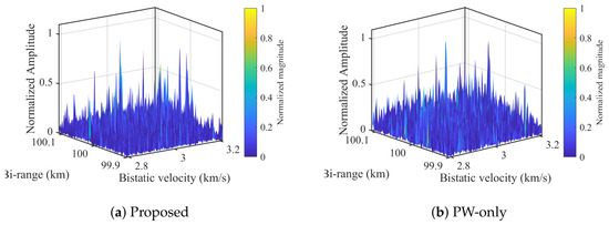
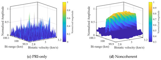
The target scenes used in these simulations are summarized in Table 4. Figure 5, Figure 6 and Figure 7 evaluate two-target separation in three representative scenes: same velocity with different range, same range with different velocity, and a close pair separated in both variables. In all three scenes, the proposed method yields the cleanest separation. The gain is particularly clear in the same-range and close-pair cases, where residual $\mathrm{PW}$-induced shift or slow-time phase error causes the partial-compensation baselines to merge the two responses into a rough pedestal.

Table 4. Target scenes used in the simulations.

Scene	Target Count	Bistatic-Range-Domain Parameters
Single target	1	$({\rho }_0,v_b,a_b,j_b)=$ (200.00 km, 3200 m s−1, 40 m s−2, −12 m s−3)
Same velocity	2	(199.86 km, 3000 m s−1, 40 m s−2, −12 m s−3) and (200.18 km, 3000 m s−1, 40 m s−2, −12 m s−3)
Same range	2	(200.00 km, 2840 m s−1, 40 m s−2, −12 m s−3) and (200.00 km, 3220 m s−1, 40 m s−2, −12 m s−3)
Close pair	2	(199.97 km, 2960 m s−1, 35 m s−2, −10 m s−3) and (200.05 km, 3040 m s−1, 35 m s−2, −10 m s−3)

Figure 5. Two-target scene with the same bistatic velocity and different equivalent bistatic ranges. The proposed method resolves the two range responses most clearly.

Figure 6. Two-target scene with the same equivalent bistatic range and different bistatic velocities. Accurate slow-time phase handling is essential here, and the proposed method provides the clearest velocity separation.

Figure 7. Close-pair two-target scene. This is the most demanding separation case. Only the full joint method preserves a clear two-peak structure with useful contrast.

In Figure 5, both targets occupy the same velocity bin but different range bins. This scene is dominated by range discrimination. The proposed method resolves the two peaks cleanly, while the $\mathrm{PW}$-only and $\mathrm{PRI}$-only baselines show stronger floor fluctuations and reduced contrast. In Figure 6, the targets occupy the same range bin but different velocities; here the quality of the nonuniform slow-time accumulation becomes critical, and the proposed method again provides the sharpest dual peak. Figure 7 is the hardest case, because the targets are close in both bistatic range and velocity. The full joint compensation still reveals two dominant responses, whereas the incomplete baselines become much less interpretable.

3.4. Detection Performance

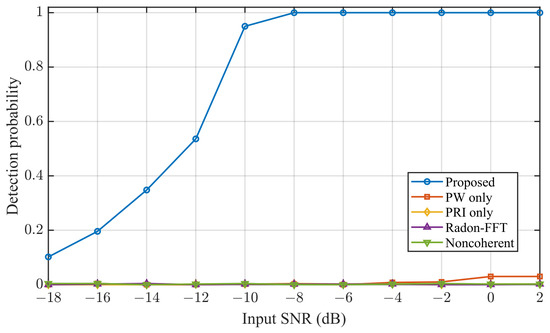
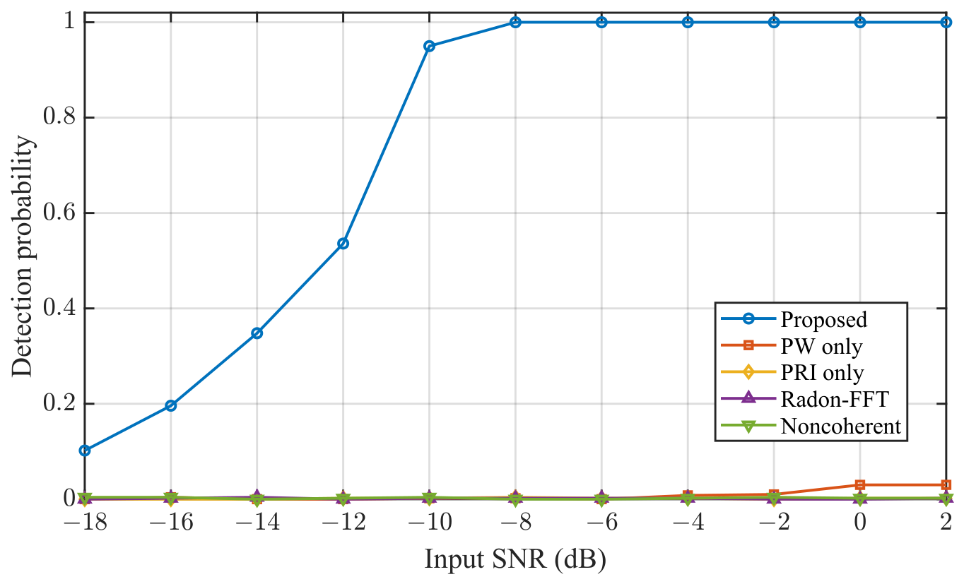
Figure 8 shows the detection probability ($P_d$) as a function of input SNR for a fixed false-alarm probability $P_{fa}={10}^{-3}$ [27], evaluated through 1000 noise-only and 500 target-present Monte Carlo trials at each SNR level. The threshold is determined empirically from the noise-only trials for each method independently, so that all methods operate at the same $P_{fa}$. The proposed method achieves $P_d>0.5$ at $\mathrm{SNR}=-12$ dB and reaches $P_d=1.0$ at $\mathrm{SNR}=-8$ dB, whereas the partial-compensation baselines and the noncoherent method remain at $P_d\approx 0$ over the entire tested SNR range. This result demonstrates that under simultaneous $\mathrm{PW}$ and $\mathrm{PRI}$ agility, the coherent gain can only be recovered when both the fast-time and slow-time mismatches are jointly compensated; correcting either effect alone is insufficient to achieve reliable detection at the specified false-alarm level.

Figure 8. Detection probability versus input SNR ($P_{fa}={10}^{-3}$, $P=96$ pulses, 1000 noise and 500 target Monte Carlo trials). Only the proposed method recovers sufficient coherent gain for reliable detection under dual agility.

3.5. SNR-Dependent Parameter-Estimation Accuracy

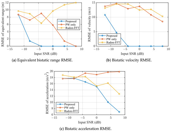
Figure 9 reports the empirical root-mean-square error (RMSE) of the grid-based estimates of equivalent bistatic range, bistatic velocity, and bistatic acceleration as a function of input SNR. Each data point is averaged over 50 independent Monte Carlo trials with independent noise realizations, and the search grid spacings are listed in Table 2; these curves correspond to a grid-based four-parameter search. In each trial, the estimate is obtained by selecting the grid point that maximizes the corresponding integration statistic. Because the true target parameters are placed exactly on the search grid (on-grid setting), the near-zero range and velocity RMSE attained by the proposed method at moderate and high SNR should be interpreted as repeated selection of the correct search cell on the prescribed grid, not as zero continuous-valued estimation error.

Figure 9. Grid-based parameter-estimation accuracy. The proposed method reaches the correct search cell more reliably than the $\mathrm{PW}$-only and Radon-FFT baselines, particularly for range and velocity. The zero-RMSE plateaus at moderate SNR indicate repeated correct grid selection rather than a continuous-valued zero-error estimator.

The proposed method consistently reduces the range RMSE first, then the velocity RMSE, and finally the acceleration RMSE as the SNR increases, reaching the correct range and velocity cells more reliably than the $\mathrm{PW}$-only and Radon-FFT baselines over the tested SNR range. The residual mismatch in the baselines moves energy away from the correct search cell, so they remain substantially worse, especially for range and velocity. The acceleration RMSE decreases more slowly, which is expected because acceleration is encoded through a higher-order slow-time phase term and is more sensitive to SNR, CPI length, and grid spacing. These curves support improved grid-based parameter-selection robustness under the stated simulation assumptions, but they should not be interpreted as a continuous-parameter performance bound. An off-grid experiment, in which the true parameters are displaced by half a grid step from the nearest grid point, would reveal the interpolation-limited estimation floor inherent in discrete-grid search and is a natural complement to the present on-grid evaluation.

4. Discussion of the Simulation

Taken together, the simulation results support the mechanism predicted by the analytical model. The schedule plot explains why fixed fast-time and uniform slow-time processing is insufficient. The single-target maps and slices show how residual mismatch appears as defocus and elevated background fluctuation in the path-sum/velocity plane. The two-target maps show that this defocus can reduce separability, especially when targets share either the same range or the same velocity. The RMSE curves then show that the recovered coherent gain improves grid-cell selection reliability as the SNR increases.

The simulations are intentionally controlled to isolate the dual-agile compensation mechanism. The waveform schedule, bistatic geometry, and calibration parameters are assumed to be known. The echo model uses point targets and additive complex white Gaussian noise, while clutter, multipath, residual synchronization errors, calibration drift, hardware distortion, and aspect-dependent scattering fluctuations are not included. Therefore, the reported gains should be interpreted as model-based validation of the proposed coherent integration framework rather than as end-to-end hardware or field-test performance.

Several practical factors may affect the method when applied beyond the current idealized setting. Bistatic ground clutter occupies isorange ellipsoids whose range–Doppler ridges differ markedly from the monostatic case [23,28], and multipath propagation through the separated transmitter–target–receiver geometry can produce ghost targets at incorrect bistatic ranges; both effects would require dedicated suppression or discrimination stages upstream of the proposed compensator. On the system side, residual clock drift and oscillator instability after cooperative calibration introduce a slowly accumulating phase error that must remain well below $\pi$ over the CPI to preserve the coherent gain [4], and spatially extended targets would spread scattering energy across multiple range cells, necessitating per-cell or multi-cell coherent processing with an appropriate scattering model [1]. Among the assumptions used in this work, two are fundamental: the waveform schedule must be known to the receiver for pulse-specific matched filtering and fast-time compensation, and cooperative calibration must establish bistatic phase coherence before slow-time accumulation. The remaining assumptions, such as point targets and AWGN, serve to isolate the dual-agile compensation mechanism and can be progressively relaxed in future extensions.

Another limitation is that the processor estimates path-sum-domain motion parameters for a single cooperative bistatic baseline. This is the appropriate observable space for the proposed derivation, but it does not remove the intrinsic geometric ambiguity of single-baseline bistatic sensing. Unique Cartesian localization would require additional baselines, angle information, or track-continuity constraints. Future simulations should include cluttered scenes, imperfect synchronization, unequal target amplitudes, multi-baseline fusion, and computationally accelerated coarse-to-fine $\mathrm{NUFFT}$ search. In addition, when the proposed coherent integration method is extended to high-resolution SAR imaging modes, advanced speckle suppression techniques [29] may serve as a useful pre-processing step to improve feature quality before coherent accumulation.

5. Conclusions

This paper addressed the coherent integration problem for cooperative bistatic radar with simultaneous PW and PRI agility. We established the signal model in the bistatic radar system to describe the delay, Doppler, acceleration, and higher-order phase terms through the bistatic path propagation distance and the bistatic projection vector. Based on this model, the effects of the two agile waveform parameters were analyzed in a unified framework. Under the fixed-bandwidth LFM assumption, PW agility changes the pulse-wise chirp rate and introduces both Doppler-dependent compressed-peak displacement and deterministic residual phase, whereas PRI agility makes the slow-time samples nonuniform and invalidates conventional uniform-PRI coherent accumulation. To compensate these effects jointly, a coherent integration method was developed by combining pulse-wise fast-time shift and phase compensation, bistatic geometric phase removal, and nonuniform slow-time coherent accumulation on the actual pulse emission times. Bistatic-range-domain ambiguity analysis and parameter-grid design rules were also derived to connect the search spacing with fast-time focusing tolerance, slow-time phase tolerance, CPI length, waveform-agility span, and bistatic geometry. Controlled simulations demonstrated that the proposed method provides more concentrated single-target focusing, clearer two-target separation, and more reliable grid-based parameter selection than partial-compensation, noncoherent, and conventional Radon-FFT baselines. These results indicate that simultaneous PW and PRI agility cannot be effectively handled by correcting only the fast-time or only the slow-time mismatch; the bistatic-range model and the two compensation stages must be used together. Future work will extend the framework to cluttered scenes, residual synchronization errors in advanced ISAR scenarios, which would help the coherent integration method be better deployed.

References

- Chen, V.C.; Martorella, M. Inverse Synthetic Aperture Radar Imaging: Principles, Algorithms and Applications; The Institution of Engineering and Technology: London, UK, 2014. [Google Scholar]
- Li, G.; Hou, Q.; Xu, S.; Chen, Z. Multi-target simultaneous ISAR imaging based on compressed sensing. EURASIP J. Adv. Signal Process. 2016, 2016, 27. [Google Scholar] [CrossRef] [Scilit]
- Palmer, J.; Homer, J.; Longstaff, I.D.; Martorella, M.; Littleton, B. ISAR imaging using an emulated multistatic radar system. IEEE Trans. Aerosp. Electron. Syst. 2005, 41, 1464–1472. [Google Scholar]
- Martorella, M.; Palmer, J.; Homer, J.; Littleton, B.; Longstaff, I.D. On bistatic inverse synthetic aperture radar. IEEE Trans. Aerosp. Electron. Syst. 2007, 43, 1125–1134. [Google Scholar] [CrossRef] [Scilit]
- Zhang, L.; Su, T.; Liu, Z.; He, X. High resolution ISAR imaging in receiver centered region area in bistatic radar. EURASIP J. Adv. Signal Process. 2013, 2013, 50. [Google Scholar] [CrossRef] [Scilit]
- Li, H.; Chen, S. General polarimetric correlation pattern: A visualization and characterization tool for target joint-domain scattering mechanisms investigation. IEEE Trans. Geosci. Remote Sens. 2026, 64, 5200417. [Google Scholar]
- Li, H.; Liu, S.; Chen, S. PolSAR ship characterization and robust detection at different grazing angles with polarimetric roll-invariant features. IEEE Trans. Geosci. Remote Sens. 2024, 62, 5225818. [Google Scholar]
- Skolnik, M.I. Radar Handbook, 3rd ed.; McGraw-Hill Education: New York, NY, USA, 2008. [Google Scholar]
- Levanon, N.; Mozeson, E. Radar Signals; John Wiley & Sons: Hoboken, NJ, USA, 2004. [Google Scholar]
- Ye, Z.; Zhu, D.; Niu, S.; Lv, J. Studies on high-resolution airborne synthetic aperture radar image formation with pseudo-random agility of interpulse waveform parameters. Remote Sens. 2024, 16, 164. [Google Scholar]
- Liu, H.; Tian, J.; Ning, C.; Cui, W.; Deng, J. Coherent integration method for random pulse repetition interval radar based on non-uniform Keystone transform and non-uniform fast Fourier transform. J. Eng. 2019, 2019, 5744–5748. [Google Scholar] [CrossRef] [Scilit]
- Stinco, P.; Greco, M.S.; Gini, F.; Rangaswamy, M. Ambiguity function and Cramér-Rao bounds for universal mobile telecommunications system-based passive coherent location systems. IET Radar Sonar Navig. 2012, 6, 668–678. [Google Scholar] [CrossRef] [Scilit]
- Tian, J.; Xia, X.-G.; Cui, W.; Yang, G.; Wu, S.-L. A coherent integration method via Radon-NUFrFT for random PRI radar. IEEE Trans. Aerosp. Electron. Syst. 2017, 53, 2101–2109. [Google Scholar]
- Pan, J.; Zhu, Q.; Bao, Q.; Chen, Z. Coherent integration method based on Radon-NUFFT for moving target detection using frequency agile radar. Sensors 2020, 20, 2176. [Google Scholar] [CrossRef] [Scilit] [PubMed]
- Lin, Z.; Wang, J.; Xu, X.; Duan, S. A novel coherent integration method for random frequency and PRI agile radar. In Proceedings of the 2023 5th International Conference on Electronic Engineering and Informatics (EEI), Wuhan, China, 30 June–2 July 2023; pp. 405–408. [Google Scholar]
- Fan, B.; Hu, W.; Du, X.; Li, Y.; Pan, J.; Bao, Q. Coherent processing for random temporal frequency agile radar by Doppler perturbed phase compensation. IEEE Trans. Aerosp. Electron. Syst. 2026, 62, 419–435. [Google Scholar] [CrossRef] [Scilit]
- Pan, J.; Chen, Z.; Hu, P.; Bao, Q.; Xu, S. Coherent integration method of high-speed target for random PRI and staggered PW radar. In Proceedings of the PIERS Spring 2019, Rome, Italy, 17–20 June 2019; pp. 1037–1040. [Google Scholar]
- Li, X.; Zhao, K.; Wang, M.; Cui, G.; Yeo, T.S. NU-SCGRFT-based coherent integration method for high-speed maneuvering target detection and estimation in bistatic PRI-agile radar. IEEE Trans. Aerosp. Electron. Syst. 2024, 60, 2153–2173. [Google Scholar]
- Xu, J.; Yu, J.; Peng, Y.-N.; Xia, X.-G. Radon-Fourier transform for radar target detection, I: Generalized Doppler filter bank. IEEE Trans. Aerosp. Electron. Syst. 2011, 47, 1186–1202. [Google Scholar] [CrossRef] [Scilit]
- Perry, R.P.; DiPietro, R.C.; Fante, R.L. SAR imaging of moving targets. IEEE Trans. Aerosp. Electron. Syst. 1999, 35, 188–200. [Google Scholar] [CrossRef] [Scilit]
- Fessler, J.A.; Sutton, B.P. Nonuniform fast Fourier transforms using min-max interpolation. IEEE Trans. Signal Process. 2003, 51, 560–574. [Google Scholar] [CrossRef] [Scilit]
- Richards, M.A. Fundamentals of Radar Signal Processing, 2nd ed.; McGraw-Hill Education: New York, NY, USA, 2014. [Google Scholar]
- Cherniakov, M. Bistatic Radar: Emerging Technology; John Wiley & Sons: Chichester, UK, 2008. [Google Scholar]
- Derham, T.; Doughty, S.; Baker, C.; Woodbridge, K. Ambiguity functions for spatially coherent and incoherent multistatic radar. IEEE Trans. Aerosp. Electron. Syst. 2010, 46, 230–240. [Google Scholar] [CrossRef] [Scilit]
- Hussain, M.G.M. Ambiguity functions for monostatic and bistatic radar systems using UWB throb signal. IEEE Trans. Aerosp. Electron. Syst. 2011, 47, 1710–1726. [Google Scholar] [CrossRef] [Scilit]
- Tsao, T.; Slamani, M.; Varshney, P.; Weiner, D.; Schwarzlander, H.; Borek, S. Ambiguity function for a bistatic radar. IEEE Trans. Aerosp. Electron. Syst. 2015, 33, 1041–1051. [Google Scholar]
- Kay, S.M. Fundamentals of Statistical Signal Processing, Volume II: Detection Theory; Prentice Hall: Upper Saddle River, NJ, USA, 1998. [Google Scholar]
- Willis, N.J. Bistatic Radar, 2nd ed.; SciTech Publishing: Raleigh, NC, USA, 2005. [Google Scholar]
- Dai, L.; Chen, S. Context2Context: A zero-shot SAR image speckle filter. IEEE Trans. Geosci. Remote Sens. 2026, 64, 5204911. [Google Scholar]
Disclaimer/Publisher’s Note: The statements, opinions and data contained in all publications are solely those of the individual author(s) and contributor(s) and not of MDPI and/or the editor(s). MDPI and/or the editor(s) disclaim responsibility for any injury to people or property resulting from any ideas, methods, instructions or products referred to in the content. |
© 2026 by the authors. Licensee MDPI, Basel, Switzerland. This article is an open access article distributed under the terms and conditions of the Creative Commons Attribution (CC BY) license.