Coastal Zone Imager Sargassum Index Model Reveals the Change Details of Sargassum in Coastal Waters of China

Highlights

What are the main findings?

• An inversion model of Sargassum based on HY-1C/D CZI was proposed.
• The new model can well distinguish Sargassum from Ulva prolifera.

What are the implications of the main findings?

• This study reveals the drift path of Sargassum.
• The model can extract and monitor Sargassum in the global coastal sea environment.

Abstract

This study reveals the distribution of floating macroalgae Sargassum in the East China Sea and Yellow Sea using HY-1C/D Coastal Zone Imager (CZI) data. A new inversion model, utilizing green and near-infrared bands, was developed for the 50 m resolution CZI data. This model effectively distinguishes Sargassum from Ulva prolifera and is effective in turbid coastal waters. Sargassum spatiotemporal distribution and drift patterns over five years were analyzed. Key findings demonstrate that (1) floating Sargassum exhibits distinct spatiotemporal distribution patterns. Sargassum initially emerges along Zhejiang’s eastern coast in February. During March and April, it concentrates east of Hangzhou Bay. While in May, Sargassum appears in the Yellow Sea, and is distributed near the Shandong Peninsula by June. Small patches of Sargassum are also found in the Yellow Sea from November to January. (2) Its distribution is influenced by various factors like nutrients, temperature, salinity, currents, and winds. Suitable nutrients, temperature, and salinity promote growth, while currents and winds, particularly in April–May, drive its northward drift from the East China Sea into the Yellow Sea. The Yellow Sea population originates from both drifting populations and local growth. (3) This research highlights the utility of HY-1C/D satellite data in coastal zone research, facilitating ecological monitoring and protection.

1. Introduction

Sargassum, a fast-growing brown macroalgae, is rich in antioxidants, carotenoids, and phenols, including the well-characterized anticancer ingredient fucoxanthin. This genus exhibits a global distribution in temperate and tropical shallow waters [1]. Seaweeds of the genus Sargassum are distributed across the three major seaweed zones along the coast of China [2,3]. Their species diversity and horizontal distribution exhibit a pattern of decreasing abundance in the north and increasing abundance in the south [4]. As the Sargassum grows, the increasing buoyancy of its air bladders may eventually exceed the fixation force of the Sargassum anchor. With the combined effects of wind, waves, currents, and the buoyancy provided by the air bladders, the Sargassum can detach from its substrate and remain afloat [5,6]. The floating Sargassum can drift at sea for one to five months, traveling hundreds of kilometers beyond its natural coastal distribution range [7].

The life cycle of the floating macroalgae Sargassum is roughly divided into four stages: resting period, growth phase, reproductive stage, and senescence phase. The primary season for Sargassum blooms in the East China Sea spans March to May, with rapid growth occurring in March–April and reproduction in April–May, followed by algal senescence and degradation [8]. The annual growth cycle of Sargassum in the Yellow Sea comprises four distinct phases: autumn reproduction, winter fixation, spring emergence and floating, and summer senescence [9]. Extensive field observations and remote sensing analyses have demonstrated that macroalgae blooms in the East China Sea and South Yellow Sea are predominantly Sargassum during February to mid-May [10]. However, during late May and June, floating Ulva prolifera undergoes rapid proliferation, ultimately displacing Sargassum as the dominant macroalgae bloom in the South Yellow Sea [11], while floating Sargassum enters terminal senescence. The growth patterns of floating Ulva prolifera and floating Sargassum exhibit distinct temporal separation with partial overlap. Ulva prolifera active proliferation occurring during May–June and subsequent senescence in July–August [12,13,14]. In contrast, floating Sargassum primarily reproduces from February to May and declines in June [10]. When the growth cycles of the two algae overlap (mid-May to June), because Ulva prolifera interferes with the extraction of Sargassum, it is necessary to consider distinguishing the two algae.

Sargassum exerts dual effects on the marine ecological environment, presenting both ecological benefits and challenges. On the positive side, Sargassum plays a crucial role in supporting fisheries [5]. As a major component of offshore algal fields and submarine forests [6], Sargassum provides habitats, feeding grounds, spawning sites, and shelter from predators for various marine invertebrates and fish [15]. Additionally, Sargassum is essential for the construction of marine pastures and the development of large-scale fisheries. Sargassum fields act as natural coastal buffers, attenuating extreme weather impacts, stabilizing shorelines, protecting vegetation growth, and reducing soil erosion [16]. They also contribute to seawater purification. On the negative side, the ecological phenomenon in which floating brown algae of the genus Sargassum change the color of seawater as a result of rapid growth or high concentrations of biomass is known as a “golden tide”, which can be harmful to marine ecosystems and human activities [17]. The golden tide exacerbates seawater eutrophication, disrupting the survival and reproduction of aquatic species. Massive algae blooms also deplete oxygen in the water, threatening the survival of marine organisms [18].

Marine ecological disasters caused by large-scale floating algal outbreaks have frequently occurred in the Yellow Sea and East China Sea in recent years [19], severely impacting the economic activities and ecological environment of coastal cities. Considering these impacts, employing remote sensing methods to monitor and research the macro-floating algae Sargassum in the Yellow Sea and East China Sea, and investigating the potential influencing factors of floating macroalgae Sargassum is essential for maintaining the balance of marine ecosystems while promoting the sustainable development of the marine economy.

In recent years, remote sensing techniques have been widely applied to study the distribution of the floating macroalgae Sargassum. In the early stage, the 300 m resolution Medium Resolution Imaging Spectrometer (MERIS), combined with the Maximum Chlorophyll Index (MCI) method, proved effective for Sargassum monitoring [20]. However, the termination of MERIS operations in 2012 created significant data gaps in continuous monitoring. In the intermediate phase, prior researchers established the floating algae index (FAI) [21]. There is no effective cloud-masking method for FAI, so clouds are not masked in the imagery. To overcome this difficulty, an alternative FAI (AFAI) was developed, where clouds can be masked through band combinations [22]. The FAI and AFAI methods utilize 250 m, 500 m, and 1 km resolution data from Moderate Resolution Imaging Spectroradiometer (MODIS) instruments, and the FAI algorithm requires short-wave infrared bands, which are not available on all satellites, and both suffer from medium-low spatial resolution limitations. In the modern phase, the Virtual-Baseline Floating Macroalgae Height (VB-FAH) index utilizes the 30 m resolution TM and ETM+ data and HJ-1 data [23]. Although Landsat and HJ-1 series satellites offer improved 30 m spatial resolution, the 16-day revisit period of Landsat and their small observation coverage are still constraints for frequent and large-scale monitoring.

Beyond the previously mentioned methods, researchers have developed various spectral indices for detecting macro-floating Sargassum, including the Fluorescence Line Height (FLH) [24], Surface Algal Bloom Index (SABI) [25], Green Algae Index (GAI) [26], Ulva prolifera and Sargassum Index (USI), Sargassum Index (SI) [27], Normalized Difference Vegetation Index (NDVI) [28], and Difference Vegetation Index (DVI) [29]. However, these algorithms present several technical limitations. The NDVI, DVI, and USI algorithms exhibit sensitivity to environmental conditions, resulting in unstable index values for the same algal species across different observations. This variability prevents the use of fixed thresholds for temporal analyses. Nevertheless, the vegetation indices can widen the difference between the absorption and reflection valleys in the spectral curves of Ulva prolifera or Sargassum, partially reducing the effects of the atmosphere and clouds, and to a certain extent, enhancing useful information and removing noise [28]. The FLH algorithm faces particular challenges in distinguishing Ulva prolifera from Sargassum due to the absence of distinct fluorescence peaks in the visible spectrum for these species. Furthermore, medium-resolution sensors (250–1000 m) such as MODIS and VIIRS typically have short revisit periods (about 1–2 days) when acquiring data [30], while Landsat8 OLI and Sentinel-2 MSI offer high spatial resolution (30 m and 10–20 m) but have longer revisit periods (16 days and 3–7 days) [31].

Due to the limitations of previous methods and the inadequacies of foreign satellite data, there is an urgent need to develop techniques that can effectively extract and differentiate the floating macroalgae Sargassum from the floating macroalgae Ulva prolifera using HY-1C/D CZI data from domestic satellites.

Chinese remote sensing satellites HY-1C/D possess dual characteristics of high resolution and a short revisit period, which enhances the opportunity for using high-resolution satellite remote sensing to observe Sargassum. The Coastal Zone Imager (CZI) sensor onboard the HY-1C/D ocean color satellite is primarily designed to acquire real-time image data of sea–land interaction zones for coastal monitoring. It aims to understand the distribution patterns of suspended sediments in critical estuaries and bays and to provide real-time monitoring and early warning of marine environmental disasters [32], including sea ice [33], red tides [34], green tides [35], and pollutants. With a spatial resolution of 50 m and a swath width of approximately 1000 km, the CZI sensor offers the advantages of higher resolution and broader observation [36].

In this paper, a new algorithm is proposed to effectively distinguish floating macroalgae Sargassum from floating macroalgae Ulva prolifera based on high-resolution (50 m) HY-1C/D CZI data. In addition, the interference of thin clouds on Sargassum extraction is overcome to some extent. By analyzing HY-1C/D CZI remote sensing satellite data from 2019 to 2023, the temporal and spatial change details of floating Sargassum in the East China Sea and Yellow Sea are revealed. This study provides scientific support for the application of HY-1C/D satellites in coastal water detection.

2. Materials and Methods

2.1. Study Area

The Yellow Sea of China (Figure 1B), located in the western part of the Pacific Ocean, is classified as a marginal sea. It is mainly divided into two regions, the South Yellow Sea and the North Yellow Sea. Large floating algae are primarily distributed in the South Yellow Sea. The South Yellow Sea is a shallow, semi-enclosed sea adjacent to the Shandong Peninsula and the shallow shoals of northern Jiangsu Province in China, spanning between 32–37°N and 119–123°E. Influenced by the continental shelf, the average seawater depth is 44 m [37]. The region’s complex hydrological conditions are shaped by the Yellow Sea Warm Current, coastal currents, and the inflow of water from the Yangtze River [38]. Major coastal cities in the area include Nantong, Yancheng, Lianyungang, Qingdao, etc. The growth and development of algae have had significant impacts, severely affecting the economic activities and ecological environment of these coastal cities [39].

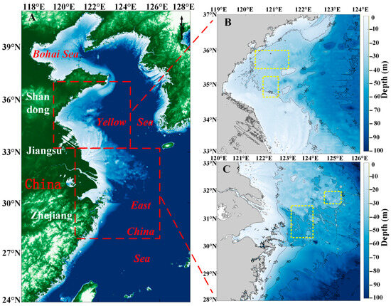
Figure 1. The study area. (A) Topographic map of the East China Sea and Yellow Sea. The red square is the study area. (B) The water depth topographic map of the South Yellow Sea. The yellow square is the location of Sargassum and Ulva prolifera in situ points. (C) The water depth topographic map of the East China Sea. The yellow square is the location of Sargassum in situ points.

The East China Sea (Figure 1C), a marginal sea bordered by mainland China, Taiwan, the Korean Peninsula, and the Japanese islands of Kyushu and the Ryukyu Islands, has its boundary with the Yellow Sea demarcated by a line connecting Cape Qidong on the northern coast near the Yangtze River estuary and the southwestern corner of Jeju Island in South Korea. The East China Sea spans between 23–33°N and 117–131°E, characterized by complex hydrological conditions, influenced by the Kuroshio Current and the Taiwan Warm Current, which flows northward into the East China Sea from the Taiwan Strait [40]. Due to its location in a subtropical region, the East Sea experiences an average annual water temperature ranging from 20 °C to 24 °C. In recent years, golden tides caused by Sargassum outbreaks have frequently occurred in the waters of the East China Sea [41].

The East China Sea and South Yellow Sea are the principal study areas of this paper (Figure 1), as they are the peak regions for Sargassum outbreaks.

2.2. Satellite Data and Processing

China launched its operational ocean water color remote sensing satellites, HY1C and HY1D, in 2018 and 2020, respectively. Equipped with the Chinese Ocean Color and Temperature Scanner (COCTS), the Coastal Zone Imager (CZI), the Ultra-Violet Imager (UVI), the Satellite-based Calibration Spectrometer (SCS), and the Automatic Identification System (AIS), these satellites have achieved global coverage of ocean water color elements twice a day and sea surface temperature four times a day [42]. The HY-1C/D satellites are specifically designed to detect ocean water color elements and water temperature, as well as their dynamic changes [36].

The HY-1C/D satellites are equipped with the CZI sensor, which has four spectral bands and a spatial resolution of 50 m (Table 1). The CZI primarily enables remote sensing observations of China and its adjacent coastal zones. The HY-1C/D satellites can complete full coverage observations of China’s near-shore areas twice every three days. Additionally, the CZI is capable of side-swinging observations, with a coverage capacity of up to 3000 km, allowing it to effectively support emergency response efforts in China’s oceans and coastal zones [32].

Table 1. Sensor characteristics of HY-1C/D CZI.

Sensor	Spatial Resolution/m	Band No.	Spectral Range/μm
HY-1C/D CZI	50	Band1 (Blue)	0.421–0.500
		Band2 (Green)	0.517–0.598
		Band3 (Red)	0.608–0.690
		Band4 (NIR)	0.761–0.891

This study utilized HY-1C/D Coastal Zone Imager (CZI) L1B and L2A data. The L1B data undergo atmospheric correction preprocessing by utilizing atmospheric characteristic parameters retrieved from L2A data, including the solar irradiance at the top of the atmosphere (F0), Rayleigh scattering optical thickness (tau_r), and ozone absorption coefficients (k_oz) to perform atmospheric correction calculations.

To minimize the impact of aerosols, we selected HY-1C/D CZI satellite data acquired on sunny and dry days, which enhances the utility of high-resolution satellite remote sensing images for Sargassum observation. HY-1C/D CZI L1B and L2A data from November to June in 2019–2023 were obtained from the National Satellite Ocean Application Center [43]. These products include blue, green, red, and near-infrared bands, which can be used to establish a Sargassum inversion model suitable for the waters of the East China Sea and Yellow Sea.

Terra-MODIS 1B imagery with a spatial resolution of 1 km from November to June in 2019–2023 was applied as a comparison with HY-1C/D CZI. The MODIS 1B data were obtained from the National Aeronautics and Space Administration’s (NASA’s) Distributed Active Archive Center (DAAC) [44]. These data were used in this study for auxiliary validation purposes. First, the MODIS 1B data underwent geometric fine correction. Subsequently, the data were resampled to 1 km resolution using the nearest neighbor method with the MCTK tool. The nearest neighbor method assigns a value to each “corrected” pixel from the nearest “uncorrected” pixel [45]. Finally, atmospheric correction was applied to the MODIS 1B data.

All calculations were performed using Python 3.8, ENVI 5.3, and ArcGIS 10.2 software.

2.3. In Situ Data

This paper collected location information for a total of 600 Sargassum sample points on 13 May 2020, 8 June 2020, 19 April 2021, 17 April 2022, 22 June 2023 around 10:30 AM and 200 Ulva prolifera sample points on 8 June 2020, 22 June 2023 around 10:30 AM which correspond to the overpass time of the HY-1C/D satellite (Figure 1B,C). The location information for the Sargassum and Ulva prolifera sample points was recorded.

The sample points were divided randomly into three groups, including the modeling group (200 Sargassum sample points) for establishing a model for preliminary extraction of Sargassum, the threshold dividing group (100 Sargassum sample points and 100 Ulva prolifera sample points) for determining optimal thresholds to distinguish Sargassum from Ulva prolifera, and the validating group (300 Sargassum sample points and 100 Ulva prolifera sample points) for assessing the accuracy of model extraction.

2.4. Measured Spectra of Sargassum

The spectral measurement of Sargassum follows the same method as terrestrial vegetation, namely the vertical measurement approach. The process involves preparing an experimental bucket, seawater, and a spectroradiometer. The experimental bucket is a transparent plastic container with a diameter of 30 cm and a depth of 50 cm. The seawater used is natural seawater collected for the experiment, and the light source is natural sunlight. Measurements are conducted on clear, low-wind days in an open area on campus free of tall surrounding buildings. The measurement period spans from 9:00 AM to 3:00 PM. Since Sargassum can suspend at certain depths below the sea surface, this study employs laboratory spectral measurement methods to obtain its spectral data. For each measurement, the number of curves recorded for the diffuse reflectance reference panel, seawater, skylight, and Sargassum in seawater exceeds 10.

We measured the Sargassum spectral by using two fresh Sargassum samples provided by Zhejiang Ocean University with the SVC HR-1024i geophysical spectrometer (Spectra Vista Corporation, Poughkeepsie, NY, USA). The first sample was collected from Taohua Island on 9 May 2024, named “Tested Sargassum 1”, and the second on 7 July 2024, named “Tested Sargassum 2”. “Tested Sargassum 1” was tested under different conditions: dry Sargassum (not soaked in seawater), floating Sargassum, and decaying Sargassum. “Tested Sargassum 1” was used for floating Sargassum measurements. Before each measurement, the water in the bucket was thoroughly stirred, after which the spectral curves of Sargassum were recorded. During spectral data processing, curves with abnormally high values were discarded, and those with relatively low and concentrated values were retained. The remaining spectral measurements were then averaged.

2.5. Performance Metrics

To evaluate the performance of the developed model, we utilized a common method of accuracy assessment for ground object target classification, namely, the confusion matrix method [46]. Three evaluation indicators were calculated according to the error matrix, including precision, recall, and F1-score [47]. Precision denotes the probability that the pixels were identified as their actual classes. Recall refers to the probability of those labeled pixels being identified correctly. The F1-score provides an accuracy indicator specific to a class by incorporating precision and recall. The three indicators can be expressed as follows:

$${\mathrm{Precision}}_{\mathrm{i}}={\displaystyle \frac{\mathrm{TP}}{\mathrm{TP}+\mathrm{FP}}}$$

(1)

$${\mathrm{Recall}}_{\mathrm{i}}={\displaystyle \frac{\mathrm{TP}}{\mathrm{TP}+\mathrm{FN}}}$$

(2)

$${\mathrm{F}1\text{-}\mathrm{score}}_{\mathrm{i}}=2\times {\displaystyle \frac{{\mathrm{Precision}}_{\mathrm{i}}\times {\mathrm{Recall}}_{\mathrm{i}}}{{\mathrm{Precision}}_{\mathrm{i}}+{\mathrm{Recall}}_{\mathrm{i}}}}$$

(3)

where TP (True Positive) are pixels correctly identified as Sargassum or Ulva prolifera, TN (True Negative) are pixels correctly identified as non-Sargassum or non-Ulva prolifera, FN (False Negative) are pixels that are actually Sargassum or Ulva prolifera but misidentified as non-Sargassum or non-Ulva prolifera, and FP (False Positive) are pixels that are actually non-Sargassum or non-Ulva prolifera but misidentified as Sargassum or Ulva prolifera.

2.6. Reanalysis Data

To explore the distribution and drift patterns of Sargassum, we also analyze Sea Surface Temperature (SST, °C) data, Sea Surface Salinity (SSS, ‰) data, Ocean current (m/s), and Wind speed (m/s) data (Table 2). The combination of these data and methods reveals the distribution patterns of Sargassum [48]. Meanwhile, these materials and techniques enable the analysis of Sargassum’s drift patterns.

Table 2. Data sources and related information.

Filed	Data Source	Spatio-Temporal Resolution	Resources
SST (°C)	Global Ocean Physics Analysis	0.083° (~9 km)/monthly	https://doi.org/10.48670/moi-00021
SSS (‰)	Global Ocean Physics Analysis	0.083° (~9 km)/monthly	https://doi.org/10.48670/moi-00021
Ocean current (m/s)	Global Ocean Physics Analysis	0.083° (~9 km)/monthly	https://doi.org/10.48670/moi-00021
10 m wind (m/s)	ERA5 monthly averaged data on single levels from 1940 to the present	0.25° (~25 km)/monthly	https://doi.org/10.24381/cds.f17050d7

The sources of oceanic and atmospheric data, along with relevant information, are provided in Table 2.

3. Results

3.1. Establishment of the Sargassum Inversion Model

3.1.1. Analysis of Spectral Characteristics of Sargassum

The spectral characteristics of Sargassum serve as the primary basis for extracting Sargassum. To retrieve Sargassum information from remote sensing images, this study measured the spectral reflectance of different Sargassum, including floating, dry, and decayed Sargassum and seawater, obtaining spectral curves for each (Figure 2A). Additionally, spectral curves of Ulva prolifera measured in previous studies were analyzed [27]. Based on the spectral curves, the overall spectral reflectance of Sargassum and Ulva prolifera is significantly higher than that of seawater. The reflectance of Sargassum and Ulva prolifera in blue and red bands has little difference. Ulva prolifera exhibits a distinct reflection peak in the green band, but Sargassum shows no significant change in the green band (Figure 2B). As the wavelength increases, both Sargassum and Ulva prolifera display a prominent ‘red edge’ phenomenon in the near-infrared band, consistent with Hu’s research results [49,50]. As shown in Figure 2, the sensitive bands of Sargassum are the green band and the near-infrared band. The green band is important for distinguishing Sargassum from Ulva prolifera.

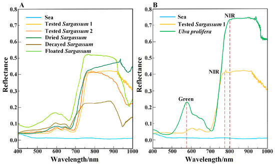
Figure 2. Spectral reflectance of Sargassum, Ulva prolifera, and seawater. (A) Measured spectral reflectance of different status Sargassum and seawater. “Tested Sargassum 1” is the sample of Sargassum collected from Taohua Island on 9 May 2024; “Tested Sargassum 2” is the sample of Sargassum collected from Taohua Island on 7 July 2024. (B) The Ulva prolifera spectra reflectance sourced from the literature [10]. The Sargassum and seawater spectral reflectance were measured. The red dotted line indicates the band range of the spectral reflectance with a significant change.

3.1.2. Model Building

Based on the difference in spectral characteristics between Sargassum and Ulva prolifera, the fluorescence baseline height (FLH) [24], the floating algae index method (FAI) [21], and Virtual-Baseline Floating Macroalgae Height (VB-FAH) [23] can be referred to establish the inversion model of Sargassum by using the principle of baseline height difference in characteristic bands of these methods. The model index is based on the reflectivity line between the blue and red bands, and the height difference between the reflectivity of the green band and the baseline is used to represent the index. The model index makes full use of the relative stability of the reflectance of the blue and red baseline bands, as well as the difference in the spectral shape of the green bands of different algae. It uses the relative height difference in the reflectance of the green band to identify Ulva prolifera and Sargassum (Figure 3A). Similarly, we can use the reflectance lines of the green and near-infrared bands as the baseline, and use the height difference between the red band and the baseline to represent the index (Figure 3B).

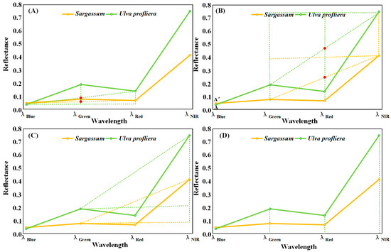
Figure 3. The simplified spectral curves of Sargassum and Ulva prolifera. (A,B) The principle of characteristic band baseline height difference. Red points indicate the intersection of the baseline and the band reflectance. (C) The difference method. (D) The ratio method.

According to the spectral characteristics of Sargassum, there is an absorption peak in the red band, a strong reflection peak in the near-infrared band, and a small reflection in other bands. The differences in band reflectance between the near-infrared bands and those of other bands of Sargassum and Ulva prolifera can be used to distinguish Sargassum from Ulva prolifera (Figure 3C). Different ground objects exhibit different reflectance values in each spectral band, and the ratio of the reflectance values in the two bands differs. Sargassum and Ulva prolifera can be distinguished by differences in their ratios (Figure 3D). The ratio method can reduce noise from atmospheric and oceanic sources across different remote sensing bands and improve the identification of algal information [28].

200 Sargassum in situ points were applied to establish the inversion model. And we extracted Sargassum from HY-1C/D CZI satellite data in the same area with the same sampling time using various models established in this paper. Table 3 shows the results of comparing the extracted Sargassum using different models with 200 in situ Sargassum points, and calculating the extraction efficiency of each model. Eight models are listed with the best extraction effect of Sargassum (Table 3).

Table 3. Band combination inversion model of Sargassum.

Number	Fitting Model	Extraction Efficiency/%
1	$R_{rc,GREEN}-{\displaystyle \frac{{\lambda }_{RED}-{\lambda }_{GREEN}}{{\lambda }_{RED}-{\lambda }_{BLUE}}}{R}_{rc,GREEN}-{\displaystyle \frac{{\lambda }_{GREEN}-{\lambda }_{BLUE}}{{\lambda }_{RED}-{\lambda }_{BLUE}}}{R}_{rc,NIR}$	80.61
2	${\displaystyle \frac{{\lambda }_{RED}-{\lambda }_{GREEN}}{{\lambda }_{NIR}-{\lambda }_{GREEN}}}{R}_{rc,NIR}-R_{rc,RED}-{\displaystyle \frac{{\lambda }_{NIR}-{\lambda }_{RED}}{{\lambda }_{NIR}-{\lambda }_{GREEN}}}{R}_{rc,GREEN}$	84.41
3	${\displaystyle \frac{R_{rc,NIR}-R_{rc,BLUE}}{{\lambda }_{NIR}-{\lambda }_{BLUE}}}$	88.22
4	${\displaystyle \frac{R_{rc,NIR}-R_{rc,GREEN}}{{\lambda }_{NIR}-{\lambda }_{GREEN}}}$	91.36
5	${\displaystyle \frac{R_{rc,NIR}-R_{rc,RED}}{{\lambda }_{NIR}-{\lambda }_{RED}}}$	90.97
6	${\displaystyle \frac{R_{rc,NIR}}{R_{rc,BLUE}}}$	85.99
7	${\displaystyle \frac{R_{rc,NIR}}{R_{rc,BLUE}}}-R_{rc,RED}$	81.48
8	${\displaystyle \frac{R_{rc,GREEN}\times R_{rc,NIR}}{R_{rc,RED}}}$	90.62

The extraction efficiency analysis in Table 3 indicates that the model based on a model of the B2 and B4 band combination provides the highest accuracy, with an extraction efficiency of 91.36%. Consequently, the Sargassum inversion model (Equation (4)) is created and named HY-1C/D CZI Sargassum Index (HSI).

$$\mathrm{HSI}={\displaystyle \frac{{\mathrm{R}}_{\mathrm{rc},\mathrm{NIR}}-{\mathrm{R}}_{\mathrm{rc},\mathrm{GREEN}}}{{\mathrm{\lambda }}_{\mathrm{NIR}}-{\mathrm{\lambda }}_{\mathrm{GREEN}}}}$$

(4)

R_rc,GREEN and R_rc,NIR are the reflectance of green and near-infrared bands observed by CZI. λ_GREEN and λ_NIR are the center wavelengths of green and near-infrared bands on CZI. HSI is HY-1C/D CZI Sargassum Index.

3.1.3. Threshold Division

During late May through June, the growth cycles of Sargassum and Ulva prolifera overlap in the South Yellow Sea [27], resulting in their co-occurrence. Ulva prolifera began to reproduce extensively [51], becoming the dominant macroalgae in the region [11], while Sargassum was in a state of decline. This requires consideration of Ulva prolifera’s interference in Sargassum extraction. Since Ulva prolifera has spectral properties similar to Sargassum, thresholds are applied to better distinguish Sargassum from Ulva prolifera. The location information of 100 Sargassum in situ points and 100 Ulva prolifera in situ points was applied for threshold division. The 200 HSI values of the same location points were obtained based on the HY-1C/D CZI satellite data with the same sampling time, and these values were analyzed. These 200 HSI values correspond to 200 in situ point positions and algae properties (Sargassum or Ulva prolifera). Therefore, the threshold range of Sargassum and Ulva prolifera can be found through comparative analysis. According to the calculated HSI value, the average HSI value of Ulva prolifera is 0.413, and the values are mainly concentrated between 0.02 and 0.85. The average HSI of Sargassum is 0.939, and the values are mainly concentrated between 0.85 and 1.19. A threshold for the Sargassum inversion model is proposed, dividing the modeled values into two parts (Figure 4). The first part corresponds to the Sargassum threshold range of [0.8528, 1.1913], with the second part corresponding to the Ulva prolifera threshold range of [0, 0.8528].

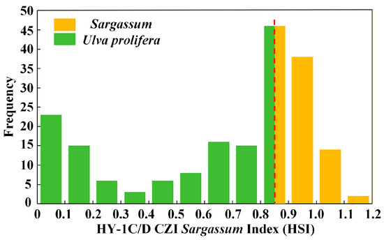
Figure 4. The HSI value distribution frequency of Sargassum and Ulva prolifera. The abscissa is the HSI value. The ordinate is the frequency of occurrence of the HSI value. The red dotted line represents the threshold value.

3.2. Validation

When there was only Sargassum before the emergence of Ulva prolifera, 100 Sargassum in situ points were applied to compare the extraction accuracy with other methods. The results demonstrate that HSI surpasses NDVI, AFAI, and USI across all key classification metrics. Specifically, HSI achieves exceptional performance with a recall of 0.930, precision of 0.939, and F1-score of 0.934 (Table 4). This indicates its balanced capability in accurately identifying true Sargassum while maintaining false positives. Those high accuracy values indicate the good performance of our developed method.

Table 4. Accuracy assessment of Sargassum inversion methods.

Method	Precision	Recall	F1-Score
HSI	0.939	0.930	0.934
NDVI	0.798	0.790	0.794
AFAI	0.871	0.880	0.875
USI	0.881	0.890	0.885

When Sargassum and Ulva prolifera coexisted, 100 Sargassum in situ points and 100 Ulva prolifera in situ points were applied to validate the model (Figure 5A). Three evaluation indicators were calculated according to the error matrix, including precision, recall, and F1-score (Figure 5C) [47]. The HSI model was successfully used to detect 90 out of 100 in situ points of Sargassum (Figure 5B). Both precision indexes for Sargassum and Ulva prolifera reached above 90%. The recall indicators were calculated to be 90.0% and 93.0% for Sargassum and Ulva prolifera, respectively. Correspondingly, their F1-score values were 90.5% and 92.5%. These high accuracy values indicate the good performance of our developed model to distinguish Sargassum from Ulva prolifera.

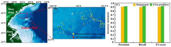
Figure 5. (A) The study area. The red square is the location of the Sargassum and Ulva prolifera in situ points. (B) The location of successful detection Sargassum points and missed detection Sargassum points by the HSI model. (C) Three evaluation indicators, precision, recall, and F1-score, for the Sargassum and Ulva prolifera pixels were calculated by using our developed model.

Furthermore, the distribution of Sargassum on the HY-1C/D CZI true-color satellite images (Figure 6A1(a1–d1)) is essentially consistent with the Sargassum obtained using the HSI model (Figure 6A2(a2–d2)). Meanwhile, the HSI method is able to extract Sargassum (Figure 6B2(e2,f2)) covered by thin clouds. 100 Sargassum in situ points were observed in the study area (Figure 6B1(e1,f1)) under thin cloudy skies. And the location information of these points was recorded. On the CZI satellite data extraction results, Sargassum was extracted at 84 locations (Figure 6B2(e2,f2)) corresponding to the same locations. This indicates that the method can monitor Sargassum under thin cloud conditions.

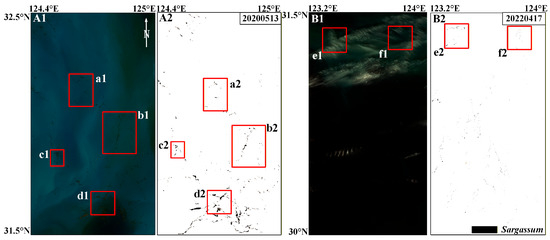
Figure 6. The distribution of Sargassum. (A1,B1) HY-1C/D CZI satellite true color images. (A2,B2) Sargassum extracted based on HY-1C/D CZI satellite data by HSI. (a1–d1,a2–d2) The distribution of Sargassum. (e1,e2,f1,f2) Sargassum was observed under thin cloudy skies.

The Sargassum inversion model developed in this study primarily utilizes the green and near-infrared bands, which are available on most satellites. It is capable of extracting Sargassum even under thin cloud cover and demonstrates high inversion accuracy. Furthermore, during the Ulva prolifera outbreak period, when Sargassum is scarce, the model can effectively distinguish Sargassum from Ulva prolifera.

3.3. Distribution Characteristics of Sargassum

Based on the newly established Sargassum inversion model, the distribution details of the floating macroalgae Sargassum in the offshore areas of the East China Sea and Yellow Sea are analyzed for the period 2019–2023.

Floating Sargassum exhibits significant spatiotemporal change features from February to June and November to January (Figure 7 and Figure 8). Sporadic floating Sargassum is detected in February in the eastern waters of Zhejiang Province. At the initial stage of the outbreak, Sargassum displays a discrete distribution on remote sensing images, appearing as small patches, and the coverage area is nearly 3 km² (Figure 7(a2,c4) and Figure 8(a2,b2)). By March, substantial floating Sargassum is observed in Hangzhou Bay’s eastern waters, reaching a mean coverage area of 26.27 km² (Figure 7(a3,b3,c5) and Figure 8(a3,b3)). During April, the coverage of Sargassum continues to expand, with an average coverage area of 44.21 km² (Figure 7(a4,b4,b5,c6) and Figure 8(a4,b4)). In May, the center of Sargassum shifts northwestward and is primarily distributed in the offshore waters of Jiangsu province, and the coverage area begins to decrease to about 37.32 km² (Figure 7(a5,a6,b6,c7,c8) and Figure 8(a5,a6,b5)). By June, the floating Sargassum appears in the southern waters of the Shandong Peninsula, with a significantly reduced coverage area of nearly 2.3 km² (Figure 7(b7) and Figure 8(b6)). From November to January, small areas of floating Sargassum are observed in the South Yellow Sea. Over time, the center of the Sargassum is discovered to be constantly turning southwards and without significant coverage change (Figure 7(a1,b1,b2,c1–c3) and Figure 8(a1,b1)).

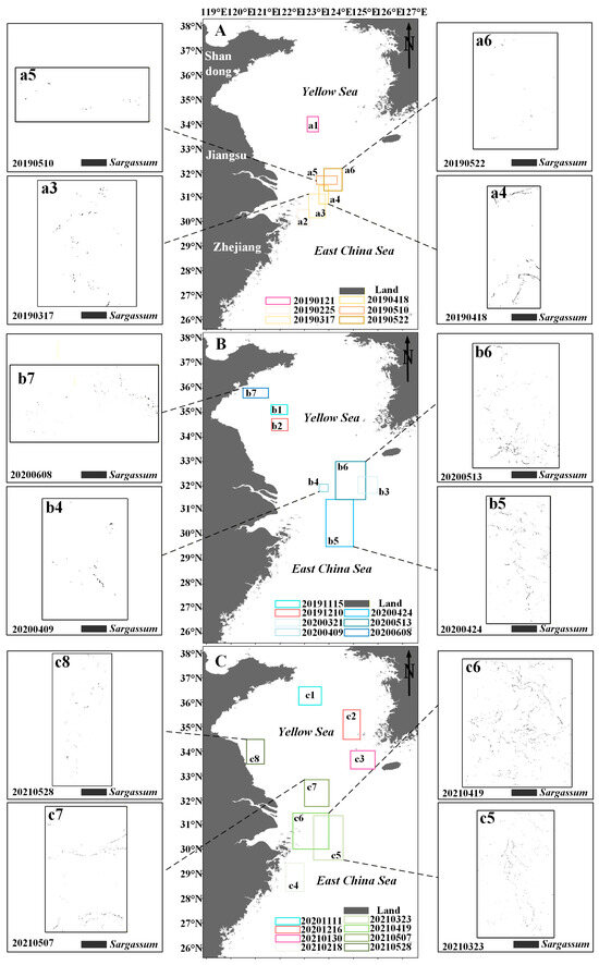
Figure 7. (A–C) The distribution of Sargassum in the study area from November to June in 2019–2021. Black boxes indicate the extraction results of Sargassum based on the HY-1C/D CZI data. (a1–a6,b1–b7,c1–c8) indicate the distribution area of Sargassum.

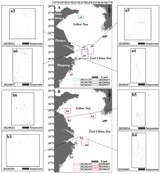
Figure 8. (A,B) The distribution of Sargassum in the study area from November to June in 2021–2023. Black boxes indicate the extraction results of Sargassum based on the HY-1C/D CZI data. (a1–a6,b1–b6) indicate the distribution area of Sargassum.

The Sargassum blooms exhibit significant change in distribution and coverage areas in the East China Sea and Yellow Sea from 2019 to 2023 (Figure 9). We observed a consistent seasonal pattern: the floating Sargassum biomass increases markedly from winter to spring, typically first appearing in February, peaking in April, and then declines around May and June. Considerable variation is observed in the Sargassum distribution area, which spans from nearly 924 km² in 2020 to approximately 28,667 km² in 2021, with peaks consistently occurring in April. The Sargassum coverage area ranges from about 1 km² in 2023 to 76 km² in 2021, with peaks also occurring in April.

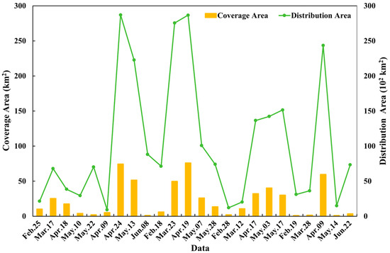
Figure 9. The variation in coverage (columns) and distribution (lines) areas of Sargassum blooms in the Yellow Sea and East China Sea during 2019 and 2023.

Generally, the continuous existence of floating Sargassum in the coastal waters of China is from February to June and from November to January (Figure 7 and Figure 8). Spatially, from February to June, the Sargassum initially emerges in the eastern waters of Zhejiang Province, subsequently occurs in the Jiangsu Province’s offshore waters, and ultimately reaches the southern Shandong Peninsula. The center of Sargassum shifts northwards from the East China Sea to the Yellow Sea. From November to January, the Sargassum primarily concentrates in the South Yellow Sea and shows a southward-moving trend of its center.

4. Discussion

4.1. The Applicability of the New Sargassum Inversion Model

The sensitive bands of the floating Sargassum inversion model are consistent with findings from previous studies (Table S1) [21,27,41], which are the green and near-infrared bands of the HY-1C/D CZI sensor. These multi-band combination approaches effectively mitigate the influence of water bodies and related environmental changes to some extent [52]. Comparative validation experimental results demonstrate that HSI surpasses both NDVI, AFAI, and USI across all key classification metrics (Precision = 93.9%, Recall = 93.0%, F1-score = 93.4%). These high-accuracy values indicate that it can effectively extract Sargassum in the East China Sea and the Yellow Sea.

Additionally, a comparison was made between the Sargassum distribution extracted based on MODIS data using the model from previous studies [53] and the Sargassum distribution extracted based on HY-1C/D CZI data using the newly developed model in this study. The results obtained from the Sargassum inversion model proposed in this research (Figure 10(A1–D1)) show high agreement with those obtained using the alternative floating algae index (AFAI) Sargassum inversion model (Figure 10(A2–D2)), further validating the feasibility of the model presented in this paper. Notably, the inversion results of the new model provide more detailed information on the distribution of Sargassum, while the AFAI results are relatively coarse and lack detailed spatial information.

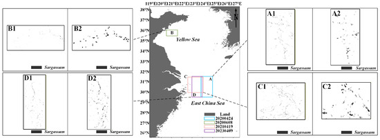
Figure 10. The distribution of Sargassum in the East China Sea and Yellow Sea from 2020 to 2023. (A–D) The distribution location of Sargassum. (A1–D1) Obtained from HY-1C/D CZI satellite data. (A2–D2) Obtained from MODIS satellite data.

The general spatiotemporal distribution pattern of floating macroalgae Sargassum obtained from the new model is largely consistent with previous findings [29,54,55], further validating the feasibility of our new model. The floating Sargassum initially emerges in the Zhejiang Province’s eastern coastal waters during February (Figure 7(a2,c4) and Figure 8(a2,b2)) [56] and subsequently occurs in the eastern waters of Hangzhou Bay in March and April (Figure 7(a3,a4,b3–b5,c5,c6) and Figure 8(a3,a4,b3,b4)) [57]. In May, the center of Sargassum shifts northwestward and is primarily distributed in Jiangsu Province’s offshore waters (Figure 7(a5,a6,b6,c7,c8) and Figure 8(a5,a6,b5)) [41] and ultimately reaches the southern waters of the Shandong Peninsula by June (Figure 7(b7) and Figure 8(b6)) [58]. From November to January, the center of the Sargassum is discovered to be constantly turning southwards in the South Yellow Sea (Figure 7(a1,b1,b2,c1–c3) and Figure 8(a1,b1)) [59].

The new model in this paper can extract Sargassum under thin clouds. Some previous methods cannot extract Sargassum under thin clouds, such as FAI [21]. Because the band combination of the green band and near-infrared band in the HSI model enhances the spectral contrast between absorption and reflection features in the vegetation curves of Ulva prolifera and Sargassum, while simultaneously mitigating atmospheric and cloud interference [28]. Experimental results show that Sargassum can be extracted under thin cloud cover conditions (Figure 6B2(e2,f2)), confirming the HSI model’s ability to extract Sargassum even under thin cloud cover.

Furthermore, the new model in this paper can eliminate the interference of Ulva prolifera and effectively extract Sargassum. Many methods in previous studies could not distinguish them, such as NDVI, FAI [21,28]. During late May and June, the growth cycles of Sargassum and Ulva prolifera overlap, resulting in their simultaneous presence in the South Yellow Sea [27]. Additionally, Sargassum and Ulva prolifera are both large floating algae and are widely distributed [60]. These require consideration of Ulva prolifera’s interference in the extraction of Sargassum. We divide the threshold by using the HSI values of Ulva prolifera and Sargassum, and verify the results after the threshold division. Experimental results demonstrate that the model effectively distinguishes Sargassum from Ulva prolifera.

The advantages of the new model in this paper mainly include the following aspects: the extraction accuracy is high, and the threshold method can be used to distinguish Sargassum from the large green algae of mixed Ulva prolifera, and can eliminate thin cloud interference, extraction Sargassum under thin cloud. In addition, compared with existing models in Table S1, the HY1C/D CZI satellite offers several obvious advantages for Sargassum monitoring. First, its medium spatial resolution (50 m) provides a balance between coverage and detail for coastal observations. Second, the dual-satellite enables unique morning–afternoon diurnal sampling capabilities, achieving an exceptional revisit frequency of ≤1.5 days. This enhances temporal resolution, significantly improving the detection of short-term dynamic processes in coastal ecosystems [42].

4.2. Factors Affecting the Distribution of Sargassum in China’s Coastal Waters

Many factors, including sea surface temperature, sea surface salinity, nutrients, ocean currents, and wind, jointly influence the growth and distribution of the floating macroalgae Sargassum [61].

In spring, the waters of the Yangtze River estuary, with suitable temperature, salinity, and rich nutrients, provide an appropriate growth environment for Sargassum. Abundant nutrients, suitable sea surface temperature, and optimal sea surface salinity promote the growth of Sargassum [62]. In spring, the Taiwan Warm Current gradually strengthens and flows northward [63], transporting phosphate-rich, hypersaline water to the nearshore waters of the Zhoushan Islands. During spring and summer, southerly winds prevail in the Zhoushan region. These winds facilitate the formation of coastal upwelling [64], which brings nutrient-rich water from the middle and lower layers of the study area into the euphotic zone. This process provides enough nutrients and favorable conditions for the growth of Sargassum [65]. This part supports the growth of Sargassum in the Yangtze Estuary in spring from the perspective of nutrients.

Temperature and Salinity significantly influence the growth and life cycle of Sargassum [66]. Sargassum exhibits high adaptability to sea surface temperature (SST) and sea surface salinity (SSS), with optimal growth occurring within a temperature range of 10–21 °C [67,68,69] and a salinity range of 20–40 PSU [62]. In the East China Sea, from February to May, the average SST ranges between 12 °C and 20 °C (Figure 11A–D,F–I), supporting Sargassum growth. Warming from March promotes photosynthetic activity, increases metabolic rates, and accelerates maturation of Sargassum [70]. However, in June, the SST over 22 °C (Figure 11E,J) exceeds thermal tolerance limits, and Sargassum disappears in the region. In the South Yellow Sea, the average SST from February to April was between 6 °C and 11 °C (Figure 11A–C,F–H), remaining below the growth threshold, with no Sargassum observed. By May, the SST reaches 14–16 °C (Figure 11C,G), suitable levels, causing Sargassum to appear in the region. However, by June, the SST over 20 °C (Figure 11D,H) induces Sargassum decline. When the temperature exceeds 20 °C, adult Sargassum stops growing or begins to senesce and lose buoyancy [71], which may explain the rapid decline in floating Sargassum observed in June. From February to June, the SSS remains in a range of 24–34 PSU (Figure 11a–j), within the suitable range for Sargassum growth. SSS displays no significant correlation with the proliferation or decline of the Sargassum [72]. Based on the above analysis, the abundant nutrients and suitable temperature and salinity conditions in the Zhoushan waters near the Yangtze River Estuary from February to May provide an ideal environment for the growth and proliferation of Sargassum. In the south Yellow Sea, the suitable temperature, salinity, and nutrients are beneficial to the growth of Sargassum in May. But in June, due to the high SST, Sargassum begins to die out.

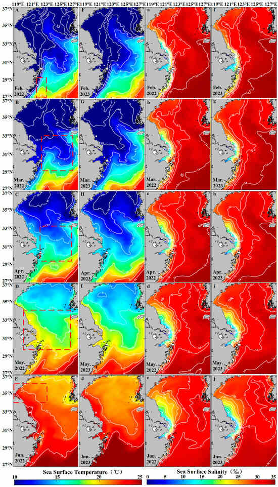
Figure 11. The hydrological element map of the study area. (A–J) The mean sea surface temperature in the study area from February to June in 2022–2023. (a–j) The mean sea surface salinity in the study area from February to June in 2022–2023. Red boxes represent Sargassum distribution areas.

The growth of Sargassum in the East China Sea and Yellow Sea indicates that Sargassum lives within a temperature range of 12–22 °C and a salinity range of 24–34 PSU. Both excessively high temperatures and low salinity inhibit the growth of Sargassum. The optimal growth temperature range is 12–18 °C, and the optimal salinity is 30–34 PSU (Figure 12).

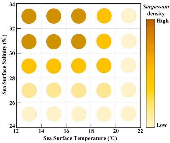
Figure 12. The density of Sargassum at different temperatures and salinities.

The distribution of Sargassum is also influenced by many environmental conditions, including ocean currents and wind fields. Surface ocean currents and wind vectors are two critical factors influencing the drift and dispersal of floating Sargassum [73,74]. Unlike other algae that attach to the seafloor for survival, Sargassum floats in the form of “rafts” on the sea surface, directly absorbing nutrients from seawater. This growth mode allows Sargassum to drift with ocean currents [75]. In February, Sargassum, influenced by the nutrient-rich waters transported by the Taiwan Warm Current, initially emerges in the eastern waters of Zhejiang Province [76]. From February to March, floating Sargassum drifts to the east of Hangzhou Bay under the influence of the onshore branching of the Taiwan Warm Current (Figure 13A,B,F,G) [40]. During March to April, the interaction of complex ocean currents and northeasterly winds promotes Sargassum’s gradual dispersal and maintains a stable distribution center (Figure 13B,C,G,H). From April to June, the ocean currents in the Yellow Sea and the East China Sea primarily flow northward (Figure 13D,E,I,J), influenced by the Yellow Sea Warm Current [77]. Concurrently, southeasterly winds prevail during this period (Figure 13d,e,i,j), further driving Sargassum to drift northwestward, eventually reaching the sea area of northern Jiangsu Province [41]. Due to the influence of the Kuroshio Current [78], Sargassum distribution cannot extend southeastward.

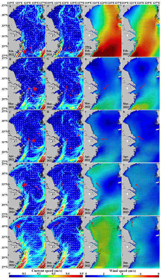
Figure 13. The hydrological element map of the study area. (A–J) The ocean currents distribution in the study area from February to June in 2022–2023. The white arrows indicate the direction and speed of the ocean current. (a–j) The wind field distribution in the study area from February to June in 2022–2023. The black arrows indicate the direction of the wind. The red arrows indicate the direction of the current and the wind. The five-pointed star represents the distribution center of Sargassum.

From the above analysis, it is evident that nutrients, sea surface temperature, sea surface salinity, ocean currents, and wind fields are the key environmental factors driving the growth, drift, and aggregation of coastal floating Sargassum. The possible drift path of floating Sargassum is primarily influenced by northward currents and southeasterly winds, resulting in a southeast-to-northwest drift pattern from February to June (Figure 14). Previous studies have also supported this drift path hypothesis [29,57].

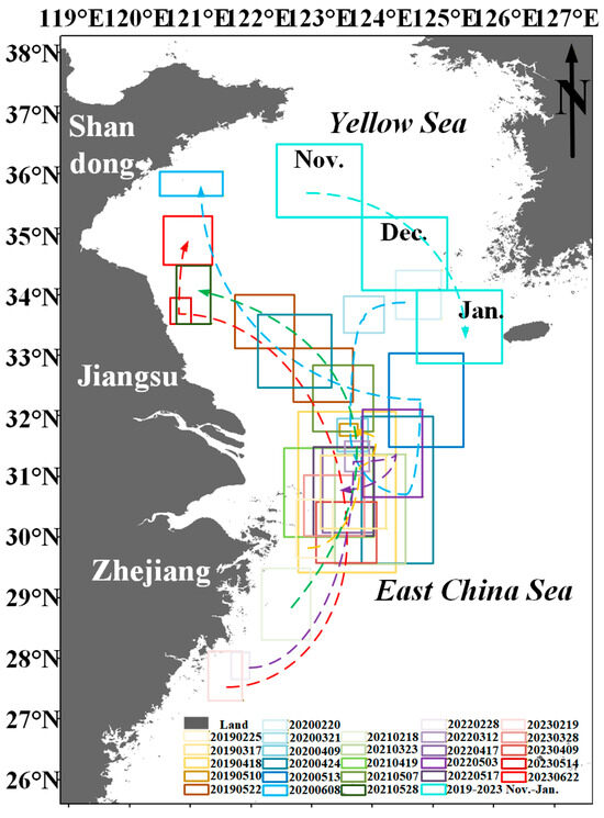
Figure 14. Drift path of Sargassum. Boxes indicate areas of Sargassum distribution from November to Jun in 2019–2023 based on HY1C/D CZI and MODIS satellite data. Dotted lines indicate possible drift paths of Sargassum.

The sequence of spatiotemporal emergence of Sargassum is that from February to June, it generally develops progressively from south to north, moving from the eastern coastal waters of Zhejiang Province to the southern waters of the Shandong Peninsula; from November to January, Sargassum gradually moves from north to south in the South Yellow Sea. In February, Sargassum initially emerges in the Zhejiang Province’s eastern waters. Under the influence of the onshore branching of the Taiwan Warm Current, the floating Sargassum drifts to the eastern waters of Hangzhou Bay in March. From March to April, under the combined effects of complex ocean currents and northeasterly winds, floating Sargassum gradually disperses, and the drift of Sargassum is not pronounced (Figure 14, light-colored frame). During May and June, the combined effects of northerly ocean currents and southeasterly winds in the Yellow Sea and East China Sea, coupled with high temperatures unfavorable for Sargassum survival in the East China Sea, cause floating Sargassum to drift northward from the eastern waters of Hangzhou Bay to the Jiangsu Province’s offshore areas. Subsequently, as the temperature continues to rise, it gradually disappears from the southern Shandong Peninsula waters by June (Figure 14, Darkened box). Since the environmental conditions in the East China Sea from February to May and the South Yellow Sea from May to June are suitable for Sargassum growth, the floating Sargassum observed on the drift path has multiple potential sources, including the drifting Sargassum from the east coast of Zhejiang Province [56,79] and local recruitment [55,80]. Additionally, floating Sargassum has a southward drifting path in the Yellow Sea from November to January [59].

Two floating Sargassum drifting paths could be independent from the East China Sea to the South Yellow Sea from February to June, and in the South Yellow Sea from November to January. Sargassum from the north could not be transported to the south of the Yangtze River mouth, possibly due to the Yangtze River ring front [81] that may serve as a “wall” to prevent particle drifting. This also suggests that Sargassum to the south of the Yangtze River ring front in February likely originated from the Zhejiang coast (Gouqi Island), which further developed into large blooms in the East China Sea from April to May [56].

5. Conclusions

In this study, a new Sargassum inversion model was established based on the combination of the green band (B2) and the near-infrared band (B4) of the HY-1C/D CZI data. This model can effectively distinguish Sargassum from Ulva prolifera and is capable of extracting Sargassum even under thin cloud cover. The distribution of floating macro-algae Sargassum in the East China Sea and Yellow Sea was analyzed (Figure 15).

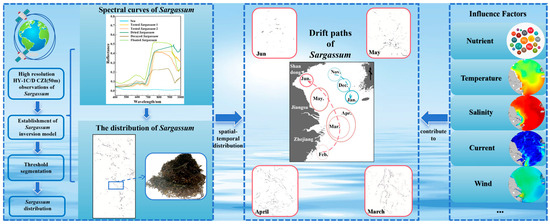
Figure 15. Coastal Zone Imager Sargassum Index model reveals the change details of Sargassum in the coastal waters of China.

The floating macroalgae Sargassum distribution in coastal waters of the Yellow Sea and East China Sea exhibits distinct temporal and spatial patterns. Floating Sargassum generally develops progressively from the eastern coast of Zhejiang Province to the southern waters of the Shandong Peninsula from February to June. It initially emerges along the Zhejiang Province’s eastern coast in February. During March and April, its center is primarily located in the Hangzhou Bay’s eastern waters. Over time, extensive floating Sargassum is observed in the South Yellow Sea in May, and by June, floating Sargassum is distributed in the southern waters of the Shandong Peninsula. In winter, small areas of floating Sargassum are observed in the South Yellow Sea, and the center of the Sargassum is constantly turning southwards from November to January.

Floating macroalgae Sargassum’s spatial and temporal distribution in the offshore waters of the Yellow Sea and East China Sea is primarily influenced by temperature, salinity, nutrients, currents, wind fields, and other factors. Abundant nutrients, suitable temperature, and salinity promote the growth of Sargassum. Ocean currents and wind fields affect the drift of floating Sargassum, which is primarily driven by northward currents and southeasterly winds in April and May, leading to its movement from the East China Sea into the South Yellow Sea. The Sargassum population in the Yellow Sea consists of two possible components: drifting from the eastern coast of Zhejiang Province and growing in local habitats.

The novelty of our research is the proposed Sargassum inversion model suitable for coastal waters. It can effectively distinguish Sargassum from Ulva prolifera and can extract Sargassum under thin cloud cover. Additionally, the HY-1C/D dual-satellite enables unique morning–afternoon diurnal sampling capabilities, achieving an exceptional revisit frequency of ≤1.5 days. It provides technical support for analyzing the distribution and drift patterns of the floating macroalgae Sargassum.

References

- Hou, M.; Bai, J.; Li, Y.; Zheng, D. Status and prospects of algae as biofertiliser. South Agric. Mach. 2023, 54, 52–54. [Google Scholar] [CrossRef]
- Li, J.; He, Y.; Deng, R.; Xiong, L.; Zhang, R. Remote sensing information extraction of Sargassum from the in-shore shallow sea in Daya Bay. Bull. Surv. Mapp. 2024, 108–114. [Google Scholar] [CrossRef]
- Seo, S.; Choi, J.M.; Park, Y.J.; Kim, K.; Park, Y.G. Origins and pathways of the floating Sargassum in the Yellow and East China Seas. Mar. Pollut. Bull. 2025, 215, 117898. [Google Scholar] [CrossRef] [PubMed]
- Huang, B.; Ding, L.; Tan, H.; Sun, G. Species diversity and distribution of genus Sargassum in China Seas. Oceanol. Limnol. Sin. 2013, 44, 69–76. [Google Scholar] [CrossRef]
- Victor, S.; Adriana, Z. Green and golden seaweed tides on the rise. Nature 2013, 504, 84–88. [Google Scholar] [CrossRef]
- Wang, D.; Jiang, Y.; Wang, X.; Wang, S.; He, E.; Zhang, Y. Research progress in ecological dynamics of golden tide dominated by Sargassum. Adv. Earth Sci. 2021, 36, 753–762. [Google Scholar] [CrossRef]
- Huang, B.; Ding, L. Golden Tide—The Past and Present Life of Floating Copper Algae in East Asia. Life World 2022, 26–27. [Google Scholar]
- Sun, J.; Zhuang, D.; Wang, T.; Chen, W.; Yang, J. Study on Sargassum herneri (Tarn) Ag around Nanji Islands. Mod. Fish. Inf. 2009, 24, 19–21. [Google Scholar] [CrossRef]
- Huang, B.; Ding, L.; Qin, S.; Fu, W.; Lu, Q.; Liu, Z.; Pang, Y.; Li, X.; Sun, Z. The Taxonomical Status and Biogeographical Distribution of Sargassum horneri with the Origin Analysis of its Drifting Population in the end of 2016 at the Western Yellow Sea. Oceanol. Limnol. Sin. 2018, 49, 214–223. [Google Scholar]
- Zheng, L.; Wu, M.; Zhao, J.; Wang, D.; Zhou, M.; Zhao, L. Remote sensing monitoring and temporal and spatial distribution characteristics of gold tide in the South Yellow Sea. Haiyang Xuebao 2022, 44, 12–24. [Google Scholar]
- Shang, J.; Zhao, Z.; Wang, W.; Ding, Y.; Song, Y. Spatial and temporal distribution characteristics of macroalgae in the Yellow Sea in 2021 based on HY-1C/D satellite data. Mar. Forecast. 2023, 40, 90–97. [Google Scholar] [CrossRef]
- He, E.; Ji, X.; Huang, H.; Wang, D.; Guo, M.; Gao, S.; Yang, J. The spatial and temporal distribution of Ulva prolifera in the Yellow Sea in recent 10 years. Mar. Forecast. 2021, 38, 1–11. [Google Scholar] [CrossRef]
- Liu, J.; Wu, M.; Zheng, L.; Xue, M.; Liu, L.; Liu, B. Spatiotemporal Characteristics of Ulva prolifera Patches in the Yellow Sea from 2011 to 2021. J. Ludong Univ. Nat. Sci. Ed. 2024, 40, 113–122. [Google Scholar] [CrossRef]
- Zhang, G.; Wu, M.; Zhao, D.; Xing, Q.; Liang, F.; Sun, X. The Inter-annual Drift and Driven Force of Ulva prolifera Bloom in the Southern Yellow Sea. Oceanol. Limnol. Sin. 2018, 49, 1084–1093. [Google Scholar] [CrossRef]
- Godoy, E.A.; Ricardo, C. Can artificial beds of plastic mimics compensate for seasonal absence of natural beds of Sargassum furcatum? ICES J. Mar. Sci. 2002, 59, S111–S115. [Google Scholar] [CrossRef]
- Amy, W.; Rusty, F. Sargassum as a natural solution to enhance dune plant growth. Environ. Manag. 2010, 46, 738–747. [Google Scholar] [CrossRef]
- Cai, J.; Geng, H.; Kong, F. Simulation study on the effect of Sargassum horneri on other harmful bloom causative species. Oceanol. Limnol. Sin. 2019, 50, 1050–1058. [Google Scholar] [CrossRef]
- Xiao, J.; Wang, Z.; Liu, D.; Fu, M.; Yuan, C.; Yan, T. Harmful macroalgal blooms (HMBs) in China’s coastal water: Green and golden tides. Harmful Algae 2021, 107, 102061. [Google Scholar] [CrossRef]
- Yu, R.; Lu, S.; Qi, Y.; Zhou, M. Progress and prospectives of harmful algae bloom studies in China. Oceanol. Limnol. Sin. 2020, 51, 768–788. [Google Scholar] [CrossRef]
- Gower, J.; Hu, C.; Borstad, G.; King, S. Ocean Color Satellites Show Extensive Lines of Floating Sargassum in the Gulf of Mexico. IEEE Trans. Geosci. Remote Sens. 2006, 44, 3619–3625. [Google Scholar] [CrossRef]
- Hu, C. A novel ocean color index to detect floating algae in the global oceans. Remote Sens. Environ. 2009, 113, 2118–2129. [Google Scholar] [CrossRef]
- Wang, M.; Hu, C. Predicting Sargassum blooms in the Caribbean Sea from MODIS observations. Geophys. Res. Lett. 2017, 44, 3265–3273. [Google Scholar] [CrossRef]
- Xing, Q.; Hu, C. Mapping macroalgal blooms in the Yellow Sea and East China Sea using HJ-1 and Landsat data: Application of a virtual baseline reflectance height technique. Remote Sens. Environ. 2016, 178, 113–126. [Google Scholar] [CrossRef]
- Xing, X.; Zhao, D.; Liu, Y.; Yang, J.; Xiu, P.; Wang, L. An overview of remote sensing of chlorophyll fluorescence. Ocean Sci. J. 2007, 42, 49–59. [Google Scholar] [CrossRef]
- Alawadi, F. Detection of surface algal blooms using the newly developed algorithm surface algal bloom index (SABI). In Proceedings of the Remote Sensing of the Ocean, Sea Ice, and Large Water Regions 2010, Toulouse, France, 20–23 September 2010. [Google Scholar] [CrossRef]
- Zhang, Z. Remote Sensing Identification of Ulva prolifra and Evolution of Green Tide in the Yellow Sea and the East China Seas. Ph.D. Thesis, East China Normal University, Shanghai, China, 2014. [Google Scholar]
- Jin, S.; Han, Z.; Liu, Y. A Remote Sensing Method for Discriminating Ulva prolifra and Sargassum. Remote Sens. Inf. 2016, 31, 44–48. [Google Scholar] [CrossRef]
- Yu, J.; Huang, H.; Shu, L.; Chen, G. Sargassum Extraction Using Remote Sensing Technology. Remote Sens. Inf. 2013, 28, 93–100+105. [Google Scholar] [CrossRef]
- Yuan, C.; Xiao, J.; Zhang, X.; Fu, M.; Wang, Z. Two drifting paths of Sargassum bloom in the Yellow Sea and East China Sea during 2019–2020. Acta Oceanol. Sin. 2022, 41, 78–87. [Google Scholar] [CrossRef]
- Kai, Y.; Jiabin, P.; Taejin, P.; Baodong, X.; Yelu, Z.; Guangjian, Y.; Marie, W.; Yuri, K.; Myneni, R.B. Performance stability of the MODIS and VIIRS LAI algorithms inferred from analysis of long time series of products. Remote Sens. Environ. 2021, 260, 112438. [Google Scholar] [CrossRef]
- Zhou, X.; Wang, J.; Zheng, F.; Wang, H.; Yang, H. An Overview of Coastline Extraction from Remote Sensing Data. Remote Sens. 2023, 15, 4865. [Google Scholar] [CrossRef]
- Cai, L.; Zhou, M.; Yan, X.; Liu, J.; Ji, Q.; Chen, Y.; Zuo, J. HY-1C Coastal Zone Imager observations of the suspended sediment content distribution details in the sea area near Hong Kong-Zhuhai-Macao Bridge in China. Acta Oceanol. Sin. 2022, 41, 126–138. [Google Scholar] [CrossRef]
- Zang, J.; Liu, J.; Yin, X.; Zeng, T.; Zhou, L. Study on sea ice classification of HY-1C satellite coastal zone imager images based on the optimal feature set. Haiyang Xuebao 2022, 44, 35–46. [Google Scholar]
- Wang, Y.; Liu, R.; Liu, J.; Ding, J.; Ye, X.; Zhao, X.; Song, D.; Ma, Y. Detection method of red tide based on the spectral features from HY-1C/D satellite: Take red Noctiluca scintillans blooms as an example. Haiyang Xuebao 2023, 45, 166–178. [Google Scholar]
- Wang, Z.; Fan, B.; Yu, D.; Fan, Y.; An, D.; Pan, S. Monitoring the Spatio-Temporal Distribution of Ulva prolifera in the Yellow Sea (2020–2022) Based on Satellite Remote Sensing. Remote Sens. 2022, 15, 157. [Google Scholar] [CrossRef]
- Liu, J.; Ye, X.; Song, Q.; Ding, J.; Zou, B. Products of HY-1C/D ocean color satellites and their typical applications. Natl. Remote Sens. Bull. 2023, 27, 1–13. [Google Scholar] [CrossRef]
- Sun, X.; Wu, M.; Xing, Q.; Song, X.; Zhao, D.; Han, Q.; Zhang, G. Spatio-temporal patterns of Ulva prolifera blooms and the corresponding influence on chlorophyll-a concentration in the Southern Yellow Sea, China. Sci. Total Environ. 2018, 640–641, 807–820. [Google Scholar] [CrossRef] [PubMed]
- Zhou, Y.; Tan, L.; Pang, Q.; Li, F.; Wang, J. Influence of nutrients pollution on the growth and organic matter output of Ulva prolifera in the southern Yellow Sea, China. Mar. Pollut. Bull. 2015, 95, 107–114. [Google Scholar] [CrossRef]
- Ma, C.; Shang, J.; Ma, W.; You, K. Assessment of the damage value of Ulva prolifera green tide of Aoshan Bay, Qingdao. Trans. Oceanol. Limnol. 2024, 46, 167–175. [Google Scholar] [CrossRef]
- Wang, J.; Si, G.; Yu, F. Progress in studies of the characteristics and mechanisms of variations in the Taiwan Warm Current. Mar. Sci. 2020, 44, 141–148. [Google Scholar]
- Qi, L.; Hu, C.; Wang, M.; Shang, S.; Wilson, C. Floating algae blooms in the East China Sea. Geophys. Res. Lett. 2017, 44, 11501–11509. [Google Scholar] [CrossRef]
- Liu, M.; Guan, L.; Liu, F.; Liu, J. Retrieval and validation of sea surface temperature from HY-1D COCTS. Natl. Remote Sens. Bull. 2023, 27, 953–964. [Google Scholar] [CrossRef]
- Online Satellite Data Dissemination System. Available online: https://osdds.nsoas.org.cn/ (accessed on 9 November 2023).
- Level-1 and Atmosphere Archive and Distribution System. Available online: https://ladsweb.modaps.eosdis.nasa.gov/ (accessed on 9 November 2023).
- Bao, W.; Yang, C.; Shao, Z.; An, G.; Liu, J.; Wu, Q. Quantitative Comparison of Three Resampling Interpolation Methods in Geometric Precision Correction. Bull. Surv. Mapp. 2009, 29, 71–72. [Google Scholar] [CrossRef]
- Fawcett, T. An introduction to ROC analysis. Pattern Recognit. Lett. 2006, 27, 861–874. [Google Scholar] [CrossRef]
- Powers, C.M.; Badireddy, A.R.; Ryde, I.T.; Seidler, F.J.; Slotkin, T.A. Silver nanoparticles compromise neurodevelopment in PC12 cells: Critical contributions of silver ion, particle size, coating, and composition. Environ. Health Perspect. 2011, 119, 37–44. [Google Scholar] [CrossRef] [PubMed]
- Li, X.; Han, Z.; Liu, X.; Jin, S.; Liu, Y. A Study of the Relationship between Processes of Enteromorpha and Sargassum and Sea Surface Temperature. Trans. Oceanol. Limnol. 2016, 44, 125–130. [Google Scholar] [CrossRef]
- Hu, C.; Feng, L.; Hardy, R.F.; Hochberg, E.J. Spectral and spatial requirements of remote measurements of pelagic Sargassum macroalgae. Remote Sens. Environ. 2015, 167, 229–246. [Google Scholar] [CrossRef]
- Qi, L.; Hu, C.; Lu, Y.; Ma, R. Spectral analysis and identification of floating algal blooms in oceans and lakes based on HY-1C/D CZI observations. Natl. Remote Sens. Bull. 2023, 27, 157–170. [Google Scholar] [CrossRef]
- Zhan, Y.; Wang, Y.; Song, K.; Rong, X.; Qu, S.; Zhu, Y. Remote sensing monitoring and analysis of the green tide in the South Yellow Sea in 2021. J. Geol. 2022, 46, 300–304. [Google Scholar] [CrossRef]
- Lv, W.; Wang, Y.; Cao, H.; Cheng, P.; Gu, X.; Ma, Z.; Li, M.; Tang, R.; Zhao, Q.; Li, X.; et al. Proximal remote sensing of dissolved organic matter in aqua-culture ponds via multi-temporal spectral correction. Front. Water 2025, 7, 1635275. [Google Scholar] [CrossRef]
- Wang, M.; Hu, C. Mapping and quantifying Sargassum distribution and coverage in the Central West Atlantic using MODIS observations. Remote Sens. Environ. 2016, 183, 350–367. [Google Scholar] [CrossRef]
- Qi, L.; Hu, C.; Barnes, B.B.; Lapointe, B.E.; Chen, Y.; Xie, Y.; Wang, M. Climate and Anthropogenic Controls of Seaweed Expansions in the East China Sea and Yellow Sea. Geophys. Res. Lett. 2022, 49, e2022GL098185. [Google Scholar] [CrossRef]
- Ding, X.; Zhang, J.; Zhuang, M.; Kang, X.; Zhao, X.; He, P.; Liu, S.; Liu, J.; Wen, Y.; Shen, H.; et al. Growth of Sargassum horneri distribution properties of golden tides in the Yangtze Estuary and adjacent waters. Mar. Fish. 2019, 41, 188–196. [Google Scholar] [CrossRef]
- Qi, L.; Cheng, P.; Wang, M.; Hu, C.; Xie, Y.; Mao, K. Where does floating Sargassum in the East China Sea come from? Harmful Algae 2023, 129, 102523. [Google Scholar] [CrossRef] [PubMed]
- Wang, Z.; Yuan, C.; Zhang, X.; Liu, Y.; Fu, M.; Xiao, J. Interannual variations of Sargassum blooms in the Yellow Sea and East China Sea during 2017–2021. Harmful Algae 2023, 126, 102451. [Google Scholar] [CrossRef]
- Zheng, L.; Wu, M.; Zhou, M.; Zhao, L. Spatiotemporal distribution and influencing factors of Ulva prolifera and Sargassum and their coexistence in the South Yellow Sea, China. J. Oceanol. Limnol. 2021, 40, 1070–1084. [Google Scholar] [CrossRef]
- Xing, Q.; Guo, R.; Wu, L.; An, D.; Cong, M.; Qin, S.; Li, X. High-Resolution Satellite Observations of a New Hazard of Golden Tides Caused by Floating Sargassum in Winter in the Yellow Sea. IEEE Geosci. Remote Sens. Lett. 2017, 14, 1815–1819. [Google Scholar] [CrossRef]
- Kong, F.; Jiang, P.; Wei, C.; Zhang, Q.; Li, J.; Liu, Y.; Yu, R.; Yan, T.; Zhou, M. Co-occurence of Green Tide, Golden Tide and Red Tides along the 35°N Transect in the Yellow Sea during Spring and Summer in 2017. Oceanol. Limnol. Sin. 2018, 49, 1021–1030. [Google Scholar] [CrossRef]
- Wang, Y.; Zhong, Z.; Qin, S.; Li, J.; Li, J.; Liu, Z. Effects of Temperature and Light on Growth Rate and Photosynthetic Characteristics of Sargassum horneri. J. Ocean Univ. China 2021, 20, 101–110. [Google Scholar] [CrossRef]
- Zou, X.; Xing, S.; Su, X.; Zhu, J.; Huang, H.; Bao, S. The effects of temperature, salinity and irradiance upon the growth of Sargassum polycystum C. Agardh (Phaeophyceae). J. Appl. Phycol. 2018, 30, 1207–1215. [Google Scholar] [CrossRef]
- Cai, L.; Tang, R.; Yan, X.; Zhou, Y.; Jiang, J.; Yu, M. The spatial-temporal consistency of chlorophyll-a and fishery resources in the water of the Zhoushan archipelago revealed by high resolution remote sensing. Front. Mar. Sci. 2022, 9, 1022375. [Google Scholar] [CrossRef]
- Sun, L.; Ke, C.; Xe, Z.; Que, J.; Tian, F. The influence of upwelling and water mass on the ecological group distribution of zooplankton in Zhejiang coastal waters. Acta Ecol. Sin. 2013, 33, 1811–1821. [Google Scholar] [CrossRef][Green Version]
- Wu, L.; Wei, Q.; Xin, M.; Wang, M.; Teng, F.; Xie, L.; Sun, X.; Wang, B. Spatial distribution patterns of nutrients and controlling mechanisms in the East China Sea during spring. Adv. Mar. Sci. 2023, 41, 622–636. [Google Scholar] [CrossRef]
- Wu, H.; Feng, J.; Li, X.; Zhao, C.; Liu, Y.; Yu, J.; Xu, J. Effects of increased CO2 and temperature on the physiological characteristics of the golden tide blooming macroalgae Sargassum horneri in the Yellow Sea, China. Mar. Pollut. Bull. 2019, 146, 639–644. [Google Scholar] [CrossRef] [PubMed]
- Shin, J.; Choi, J.G.; Kim, S.H.; Khim, B.K.; Jo, Y.H. Environmental variables affecting Sargassum distribution in the East China Sea and the Yellow Sea. Front. Mar. Sci. 2022, 9, 1055339. [Google Scholar] [CrossRef]
- Zhang, Y.; Bi, Y.; Wang, W.; Sui, Y.; Lu, K.; Feng, M.; Liang, J.; Zhou, S. Spatial Distribution Patterns of Sargassum vachellianum in Coastal Waters of Northern Zhejiang Typical Islands. Acta Hydrobiol. Sin. 2019, 43, 1114–1121. [Google Scholar] [CrossRef]
- Pang, S.J.; Liu, F.; Shan, T.F.; Gao, S.Q.; Zhang, Z.H. Cultivation of the brown alga Sargassum horneri: Sexual reproduction and seedling production in tank culture under reduced solar irradiance in ambient temperature. J. Appl. Phycol. 2009, 21, 413–422. [Google Scholar] [CrossRef]
- Choi, H.G.; Lee, K.H.; Yoo, H.I.; Kang, P.J.; Kim, Y.S.; Nam, K.W. Physiological differences in the growth of Sargassum horneri between the germling and adult stages. J. Appl. Phycol. 2008, 20, 729–735. [Google Scholar] [CrossRef]
- Choi, S.K.; Oh, H.-J.; Yun, S.-H.; Lee, H.J.; Lee, K.; Han, Y.S.; Kim, S.; Park, S.R. Population Dynamics of the ‘Golden Tides’ Seaweed, Sargassum horneri, on the Southwestern Coast of Korea: The Extent and Formation of Golden Tides. Sustainability 2020, 12, 2903. [Google Scholar] [CrossRef]
- Xu, M.; Li, Q.; Yao, D.; Zou, X.; Huang, H.; Bao, S.; Gong, C.; Zhu, J.; Mu, D. Effects of temperature, light intensity, salinity on growth and photosynthetic physiology of Sargassum ilicifolium. South China Fish. Sci. 2023, 19, 127–133. [Google Scholar] [CrossRef]
- Wang, Z.; Xiao, J.; Fan, S.; Li, Y.; Liu, X.; Liu, D. Who made the world’s largest green tide in China?—An integrated study on the initiation and early development of the green tide in Yellow Sea. Limnol. Oceanogr. 2015, 60, 1105–1117. [Google Scholar] [CrossRef]
- Tak, Y.J.; Cho, Y.K.; Seo, G.H.; Choi, B.J. Evolution of wind-driven flows in the Yellow Sea during winter. J. Geophys. Res. Ocean. 2016, 121, 1970–1983. [Google Scholar] [CrossRef]
- Kim, K.; Shin, J.; Kim, K.Y.; Ryu, J.-H. Long-Term Trend of Green and Golden Tides in the Eastern Yellow Sea. J. Coast. Res. 2019, 90, 317–323. [Google Scholar] [CrossRef]
- Choi, J.G.; Kim, D.; Shin, J.; Jang, S.W.; Lippmann, T.C.; Jo, Y.H.; Park, J.; Cho, S.W. New diagnostic sea surface current fields to trace floating algae in the Yellow Sea. Mar. Pollut. Bull. 2023, 195, 115494. [Google Scholar] [CrossRef]
- Cao, Y.; Zhu, Q. Study on the intensity and temporal and spatial variation of Yellow Sea Warm Current based on Aqua/MODIS data. Mar. Forecast. 2021, 38, 93–102. [Google Scholar] [CrossRef]
- Li, Z.; Guo, J.; Song, J.; Bai, Z.; Fu, Y.; Cai, Y.; Wang, X. Distribution, movement and generation mechanism of the mesoscale eddy around the Kuroshio in the East China Sea. J. Mar. Sci. 2022, 40, 1–10. [Google Scholar] [CrossRef]
- Komatsu, T.; Tatsukawa, K.; Filippi, J.B.; Sagawa, T.; Matsunaga, D.; Mikami, A.; Ishida, K.; Ajisaka, T.; Tanaka, K.; Aoki, M.; et al. Distribution of drifting seaweeds in eastern East China Sea. J. Mar. Syst. 2006, 67, 245–252. [Google Scholar] [CrossRef]
- Zhan, D.; Liu, W.; Xin, M.; Wang, X. A preliminary study on origin of drifting Sargassum horneri in North Yellow Sea. Trans. Oceanol. Limnol. 2022, 44, 123–127. [Google Scholar] [CrossRef]
- Liu, D.; Wang, Y.; Wang, Y.; Keesing, J.K. Ocean fronts construct spatial zonation in microfossil assemblages. Glob. Ecol. Biogeogr. 2018, 27, 1225–1237. [Google Scholar] [CrossRef]
Disclaimer/Publisher’s Note: The statements, opinions and data contained in all publications are solely those of the individual author(s) and contributor(s) and not of MDPI and/or the editor(s). MDPI and/or the editor(s) disclaim responsibility for any injury to people or property resulting from any ideas, methods, instructions or products referred to in the content. |
© 2025 by the authors. Licensee MDPI, Basel, Switzerland. This article is an open access article distributed under the terms and conditions of the Creative Commons Attribution (CC BY) license.