Highlights
What are the main findings?
- Four spectral indices were identified as important for the quantification of seagrass within and adjacent to the MSC-certified Western Australia Enhanced Greenlip Abalone Fishery. The Normalised Difference Aquatic Vegetation Index (NDAVI) and Depth Invariant Index of the blue and green bands were the most important indices.
- Similar seagrass cover and distribution were observed inside and outside of the fishery area of operation.
What are the implication of the main finding?
- The use of indices from free satellite products via Google Earth Engine workflows and automatic image annotation provides a rapidly repeatable method to support ecosystem-based fisheries management for this fishery.
- These findings may have broader applications for ecosystem monitoring across moderately deep (<20 m) fisheries and marine management areas.
Abstract
Understanding and monitoring benthic habitat distribution is essential for implementing ecosystem-based fisheries management (EBFM). Satellite remote sensing offers a rapid and cost-effective approach to marine habitat assessments; however, its application requires context-specific adjustment to account for environmental variability and differing study aims. As such, predictor variables must be tailored to the specific site and target habitat. This study uses Sentinel-2 Level 2A surface reflectance satellite imagery and stability selection via Random Forest Recursive Feature Elimination to assess the importance of remote sensing indices for mapping moderately deep (<20 m) seagrass habitats in relation to the Marine Stewardship Council-certified Western Australia Enhanced Greenlip Abalone Fishery (WAEGAF). Of the seven indices tested, the Normalised Difference Aquatic Vegetation Index (NDAVI) and Depth Invariant Index for the blue and green bands were selected in the optimal model on every run. The kernelised NDAVI and Water-Adjusted Vegetation Index also scored highly (both 0.92) and were included in the final classification and regression models. Both models performed well and predicted a similar cover and distribution of seagrass within the fishery compared to the surrounding area, providing a baseline and supporting EBFM of the WAEGAF within the surrounding marine protected area. Importantly, the use of indices from freely accessible ready-to-use satellite products via Google Earth Engine workflows and expedited ground truth image annotation using highly accurate (0.96) automatic image annotation provides a rapidly repeatable method for delivering ecosystem information for this fishery.
1. Introduction
1.1. EBFM and Habitat Assessment
Fisheries management has progressively shifted from a target-species focus toward ecosystem-based fisheries management (EBFM), which explicitly accounts for broader ecological drivers influencing fishery productivity and sustainability [1,2]. A central requirement of EBFM is a spatially explicit understanding of benthic habitats, their productivity, and their relationships with commercially important species or operations [3]. Among these, seagrass meadows and other submerged aquatic vegetation (SAV) are particularly important, providing nursery grounds and trophic support for fish and fisheries and delivering broader ecosystem services [4]. Therefore, the ability to confidently and quantitatively assess, map, and monitor these habitats with fit-for-purpose techniques that can inform the ongoing effectiveness of fisheries management arrangements and ecosystem resilience is critical [5,6,7]. Reliable and defensible habitat assessment and monitoring not only guide sustainable fisheries decision-making but also reinforce stewardship and the social licence needed to maintain public confidence in the management of marine resources [8].
1.2. Cost-Effective Habitat Assessment Tools
Although limitations exist due to the presence of water, remote sensing, particularly from satellites, offers a powerful and cost-effective approach for the assessment and monitoring of marine habitats [9]. Compared to airborne sensors, satellite data are more cost-effective and accessible, and are scalable for bioregional habitat assessments, providing a valuable resource to support ongoing marine ecosystem monitoring and management. An example satellite product is the freely available Sentinel-2 imagery operated by the European Space Agency, which consists of two satellites that together provide frequent (5-day revisit) medium-resolution (10 m) multispectral earth observation imagery [10]. The Sentinel-2 Level-2A (L2A) product, available operationally since March 2018, provides orthorectified atmospherically corrected surface reflectance imagery by accounting for atmospheric effects such as aerosols and water vapour [11]. As a ready-to-use product, L2A mitigates the need for manual atmospheric correction, offering a consistent and accessible dataset that reduces processing time. Satellite remote sensing is well-suited to the mapping and monitoring of seagrass habitats, especially shallow, monospecific, high-cover meadows that often contrast strongly with the surrounding habitat [12,13], and the combination of spatial and spectral resolution offered by Sentinel-2 makes it particularly suited for this purpose [14].
The emergence of Google Earth Engine (GEE) as a freely available cloud-based spatial analysis platform has significantly improved access to satellite remote sensing for marine resource management [15]. Established in 2010, GEE provides a continuously updated archive of satellite and geospatial datasets, including imagery from missions such as Sentinel-1, Sentinel-2, Landsat, MODIS, and VIIRS. Its cloud computing infrastructure enables users to process and analyse large datasets rapidly, perform time-series assessments, and generate reproducible workflows without relying on high-end local computing resources or extensive storage capacity. By lowering technical, processing, and infrastructure barriers, GEE allows scientists, managers, and policymakers access to timely, scalable, and reliable earth observation information, which supports monitoring, planning, and evidence-based decision-making in marine and coastal environments.
The recent development and rapid uptake of cloud-based automatic image annotation (AIA) platforms (e.g., CoralNet, ReefCloud, BIIGLE, Squidle+) has also played a critical role in streamlining marine habitat assessments by alleviating the requirement for the full manual annotation of benthic ground truth imagery [16,17,18]. These AIA platforms are browser-based interfaces that leverage machine learning algorithms to automate or semi-automate image annotation, allowing for benthic classification with high consistency and confidence metrics, whilst providing streamlined workflows that reduce processing time, minimise labour costs, enhance reproducibility, and allow access for users without data science or programming expertise [18]. In-house AIA, where data remains on secure internal servers, is also increasingly achievable and may be a requirement for commercially sensitive or proprietary imagery [19]. By accelerating image analysis and improving data quality, AIA tools facilitate large-scale, timely marine habitat assessments to inform marine resource management and spatial planning.
This combination of advances and availability in satellite imagery products, cloud-based spatial analysis platforms, and AIA tools has made robust, rapid, and repeatable marine habitat assessment increasingly achievable for scientists, resource managers, and stakeholders. Together, the emergence of these tools enables more frequent and/or more cost-effective marine habitat assessment, which allows for timely, data-driven decision-making that enhances the capacity for the stewardship of marine resources.
1.3. Remote Sensing Indices
Numerous satellite remote sensing indices, derived from various spectral band combinations, have been developed to detect and monitor the aquatic environment [20]. A large subset of these are aquatic vegetation indices (AVIs) that were modified from terrestrial vegetation applications and initially focused on emergent and floating vegetation. However, recent developments have produced indices designed specifically for submerged aquatic vegetation (SAV), including seagrass and macroalgae, with the potential for broader application in coastal and shallow marine environments. Two of the more established and widely used AVIs are the Normalised Difference Aquatic Vegetation Index (NDAVI) and the Water-Adjusted Vegetation Index (WAVI), both developed by Villa et al. (2014) to detect aquatic vegetation in very shallow lake environments (<1 m depth) [21]. NDAVI and WAVI modified the terrestrial Normalised Difference Vegetation (NDVI) and Soil-Adjusted Vegetation (SAVI) indices, respectively, by replacing the red band with the blue band to improve water penetration. In terrestrial applications, NDAVI is referred to as the blue normalised difference vegetation index (BNDVI). Although originally intended for shallow freshwater systems, NDAVI and WAVI have since been applied successfully to map seagrass and other SAV in marine environments at depths of up to ~30 m [20,22,23,24,25]. A recent refinement of NDAVI is the kernelised Normalised Difference Aquatic Vegetation Index (kNDAVI), developed by Mastrantonis et al. [25] using the kernel-based adaption of the terrestrial NDVI proposed by Wang et al. [26]. Although still in the early stages of application, kNDAVI was demonstrated to provide improved performance over NDAVI in discriminating SAV to depths of up to 30 m in various algae-dominated coastal locations across the temperate Western Australian West Coast Bioregion [25].
Several recently developed AVIs have specifically targeted submerged seagrass. One such index is the Submerged Seagrass Identification Index (SSII) proposed by Li et al. [27], who identified that shallow seagrass species may exhibit a distinctive reflectance peak between the red (Band 4: 665 nm) and red edge (Band 5: 705 nm) bands in Sentinel-2 imagery. SSII was found to be effective in discriminating submerged seagrass in shallow environments (<4 m depth); however, the authors noted that further validation is required to determine its effective depth range. In addition to SSII, Seagrass Index I (SSI-1) and Seagrass Index II (SSI-2) were developed by Liang et al. [28] using Landsat imagery and were applied to very shallow waters (<2 m depth). SSI-1 incorporates reflectance from the red, near-infrared (NIR), and shortwave infrared (SWIR1) bands, while SSI-2 uses a combination of the green and red bands. In addition, Bai et al. [29] used Landsat imagery to evaluate the Sum Green Index (SGI), which is simply the mean of the reflectance across the 500 nm to 600 nm portion of the spectrum that was developed by Lobell and Asner [30] for terrestrial applications. SGI was found to be highly accurate at distinguishing dense seagrass cover in clear water up to 4 m depth, though its performance declined with increasing turbidity and seagrass sparseness.
In addition to vegetation-specific indices, the Depth Invariant Index (DII) is a remote sensing index that has been widely used for more than three decades to discriminate benthic habitats, particularly in seagrass mapping applications [31,32,33]. Originally proposed by Lyzenga [34], DII corrects for the influence of water column depth by applying logarithmic transformations and attenuation coefficients to two spectral bands, typically selected from the visible portion of the spectrum. This transformation reduces the confounding effect of water by making the ratio of the bands invariant to changes in depth and enhancing the spectral separability of benthic features.
Despite the numerous available aquatic remote sensing indices and studies dedicated to the subject, there is no widely adopted index for remote seagrass habitat discrimination. This is primarily due to the variability in local environmental conditions, which affect spectral responses and model performance, as well as differing study objectives and target species or morphologies [35,36]. For these reasons, it is imperative that predictor variables and indices for habitat distribution models be assessed critically so that they can be tailored to the specific study environment and objective.
1.4. Fishery Background and Habitat Association
Since 2014, Rare Foods Australia Ltd. (RFA) has operated a commercial ocean ranching enterprise for greenlip abalone (Haliotis laevigata) within Flinders Bay, Western Australia. As part of the Western Australian Enhanced Greenlip Abalone Fishery (WAEGAF), RFA contributes to sustainable seafood production through the deployment of small artificial concrete habitat modules, termed “Abitats”, across a 413-hectare lease area. Juvenile abalone, reared in a land-based hatchery to 40–50 mm, are transferred to the ocean lease for grow-out. RFA maintains around 10,000 Abitats, occupying a total footprint of ~1% of the lease area, and the most recent survey estimated a standing biomass of 149 tonnes of abalone, equating to roughly 1.1 million individuals. The lease is situated within the General Use zone of the Ngari-Capes Marine Park and is adjacent to seagrass habitats, necessitating a robust environmental stewardship. RFA holds Marine Stewardship Council (MSC) certification (Standard v2.01), with specific conditions and action plans developed for the monitoring of vulnerable marine ecosystems, particularly seagrass beds, whilst also undertaking biannual stock assessments and five-yearly sediment sampling to assess nutrient dynamics.
The recent literature has highlighted the potential ecological interactions between artificial reefs and seagrass ecosystems. A study by Andskog et al. [37] demonstrated that artificial reefs in tropical systems can enhance seagrass productivity and ecosystem services, including carbon sequestration, through mechanisms such as fish aggregation. However, the applicability of these findings to moderately deep temperate systems, such as Flinders Bay, remains uncertain. Although unlikely, nutrient enrichment associated with increased abalone biomass [38] may lead to light limitation and reduced seagrass growth due to increased phytoplankton [39], underscoring the complexity of ecosystem responses to anthropogenic structures. While further research is needed to clarify these dynamics in temperate environments, the findings provide a valuable context for assessing the potential ecological outcomes from WAEGAF operations and highlight the importance of monitoring and adaptive management to ensure that seafood production aligns with broader sustainability and EBFM objectives.
1.5. Study Objectives
This study aims to review and evaluate a suite of remote sensing indices, including those specifically targeted at aquatic vegetation, for their effectiveness at predicting moderately deep (~6–22 m) seagrass habitat within and adjacent to the WAEGAF in Flinders Bay, Western Australia. The most informative indices will then be used to guide Random Forest classification and regression models to generate spatially explicit maps of seagrass distribution and abundance for the study area. These outputs will support the delivery of EBFM for the WAEGAF. Importantly, the use of indices obtained from freely available satellite imagery integrated into a cloud-based spatial analysis platform and a highly accurate automated image classifier enables a reproducible workflow that facilitates rapid marine habitat assessment and robust evidence-based decision-making by resource managers and stakeholders.
2. Materials and Methods
2.1. Study Area
The study was conducted in the western extent of Flinders Bay in the south-west region of Western Australia (Figure 1). Positioned at the confluence of the Indian and Southern Oceans, Flinders Bay is a south-facing embayment with predominant seagrass and sand habitats and occasional mixed reef assemblage characteristic of the temperate south-western Australian coastline. The area receives coloured dissolved organic matter (CDOM)-rich freshwater outflow from the Blackwood River and lies within a general use area of the Ngari-Capes State Marine Park.
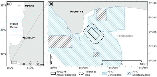
Figure 1.
Map showing the location of (a) the study area in relation to Perth and the south-west of Western Australia, and (b) Augusta and Flinders Bay with the WAEGAF area of operation, surrounding reference area, and marine protected area zoning.
The study was performed within a 15.95 km2 (1595 ha) area of Flinders Bay that was divided into two zones: (1) the central WAEGAF area of operation (4.13 km2) and (2) a surrounding reference area (11.82 km2) that extended as a 1 km buffer from the WAEGAF area of operation and represented comparable environmental and habitat conditions without WAEGAF activities (Figure 1). LiDAR-derived depth ranged from 8.3 to 19.5 m (mean = 16.6 m) in the WAEGAF area of operation, and 6.3 and 22.5 m (mean = 15.6 m) in the reference area [40].
2.2. Unsupervised Classification and Ground Truth Sampling
Cloud-free Sentinel-2 L2A surface reflectance images of the study area were retrieved through Google Earth Engine (GEE) for the 2023/24 austral summer (December–February) and assessed using a deep-false colour composite (Bands 1,2,3). Imagery acquired on 10 February 2024 (Scene ID: T50HLH) was selected for unsupervised classification due to its optimal water clarity, low CDOM-rich river water discharge, and minimal surface disturbance (e.g., wind waves) (Figure S1a). Sun-glint correction was applied following the methodology of Hedley et al. (2005) (Figure S1b) [41].
Unsupervised classification was conducted in GEE using K-means clustering with 50,000 seeds, utilising only Band 2 (blue; 490 nm). The within-cluster sum of squares (WCSS) elbow method indicated that 3–4 clusters were optimal; however, a 5-class unsupervised classification was selected, as it marginally improved the clustering performance and still allowed for sufficient within-class ground truth sampling replication in the available field time (Figures S2 and S3).
A total of 75 ground truth sampling points (referred to as “sites” herein) were randomly allocated within the study area, stratified proportional to the area of each of the 5 unsupervised classes, and separated by a minimum distance of 75 m. Sites were generated in R using the terra, sf, and dplyr packages [42,43,44]. All relevant layers were projected to WGS84/UTM Zone 50S (EPSG: 32750) prior to spatial analyses. Ground truth sampling occurred on 24 February 2025. Five replicate downward facing images (single image area = 0.66 m2) were collected at each site by a downward facing camera (DJI Osmo Action 5 Pro; 4k; 4:3; Linear) mounted on a lander 0.6 m above the benthos using a drift-drop technique over a ~30 m transect [6] (Figure 2).
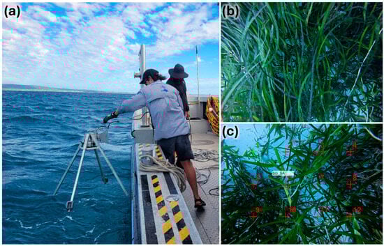
Figure 2.
Images showing (a) deployment of the downward facing lander, (b) example of a replicate downward facing image, and (c) a replicate image with 4 × 3 point grid annotation.
2.3. Ground Truth Image Annotation and Trained Classifier
With permission from Rare Foods Australia, the 375 benthic images (75 sites; 5 replicates) were imported as 4:3 (3840 × 2880) Portable Network Graphics files into the widely used automatic benthic image annotation tool, CoralNet [16]. CoralNet uses an EfficientNet-B0 machine learning model backbone that, once trained, allows for the automatic acceptance of machine-classified points over a defined confidence threshold [16]. Each image was annotated using a 12 (4 × 3) point grid overlay resulting in 60 annotated points per site. All annotation points were human confirmed without auto-acceptance (i.e., alleviation confidence threshold was set to 100%). The annotation labelset contained 62 labels from 7 functional groups that represented the habitats of the area and were aligned to the CATAMI classification scheme with the decision tree nodes pruned or collapsed to allow for the image classifier to apply single-label classification [45]. Seagrasses and frequently observed macroalgae were identified to genera where possible.
The presence of predominantly macroalgae wrack overlying and obscuring the benthic habitat was identified as a potential source of remote sensing classification error during analysis. Consideration was given to removing images with identifiable wrack; however, model accuracy was ultimately assessed using the complete set of imagery. Excluding such images would require subjective, qualitative decisions that risk introducing observer bias, while also increasing image processing time. This would ultimately reduce both the cost-effectiveness and accessibility of future assessments.
The benthic composition for each label was converted to percentage cover per site. For binary classification, sites were grouped into presence and absence of seagrass with a 20% threshold: seagrass (≥20% seagrass cover) and non-seagrass (<20% seagrass cover). The threshold was selected based on remote sensing limitations, as it is generally difficult to reliably detect seagrass cover below this level in satellite imagery.
The performance of the image classifier was evaluated from a 7/8 training and 1/8 holdout testing split of human annotated points. Accuracy, precision, recall, specificity, F1 score, and the Matthews correlation coefficient were calculated from a two-class confusion matrix (presence/absence of seagrass).
2.4. Satellite Image Pre-Processing and Index Calculation
Using the same image acquisition and pre-processing approach in GEE as the unsupervised classification, Sentinel-2 imagery captured on 6 March 2025 (Scene ID:T50HLH) was selected for supervised classification. Four aquatic vegetation indices (AVIs) were identified as suitable for further investigation (Table 1). These indices were calculated in GEE and appended as bands to the image, alongside the Sentinel-2 coastal, blue, and green bands. In addition, the Depth Invariant Index of the blue and green (DIIBG), coastal and blue (DIICB), and coastal and green bands (DIICG) were computed following the method of Lyzenga (1978) [34]. Ground truth data were filtered to include only sites characterised by 100% soft substrate (i.e., sand) to inform the attenuation coefficient required for the Depth Invariant Index calculations. Thus, the final image stack used for evaluation consisted of ten bands.

Table 1.
Summary of aquatic vegetation indices (AVIs) assessed for suitability, including their formulations and rationale for inclusion or exclusion in this study. Sentinel-2 L2A band abbreviations: B = blue (492 nm), G = green (560 nm), R = red (665 nm), NIR = near-infrared (833 nm), SWIR1 = shortwave infrared 1 (1610 nm).
2.5. Remote Sensing Indices Evaluation
To evaluate the relative contribution of the predictor variables to seagrass classification, Random Forest Recursive Feature Elimination (RF-RFE) was performed. RF-RFE is a method for feature selection that repeatedly runs RF models, ranks the importance of predictors, and removes the least important in a stepwise manner. The selection of RF was based on its widespread use for coastal mapping, in particular seagrass habitats, its robustness to overfitting and multicollinearity, and its capacity to avert overtraining [47,48]. The initial set of candidate predictors were the ten bands of the image stack that included the four selected AVIs (NDAVI, WAVI, kNDAVI, and SSI-2), as well as the coastal, blue, and green spectral bands from the imagery and their associated Depth Invariant Indices (DIIBG, DIICB, DIICG). The response variable was the seagrass binary classification (i.e., presence/absence of ≥20% seagrass cover). The LiDAR-derived DEM was not included as a predictor variable, as the temporal accessibility of this variable did not align with the satellite-derived products, making it unable to be used cost-effectively during rapid assessment.
The RF-RFE procedure used 4-fold spatial block cross-validation with block size set to 2000 m to iteratively assess model performance across all possible subsets of the predictor variables (Figure S4). A stability selection approach was used to assess the robustness of variable selection [49]. For this approach, RF-RFE was performed 100 times, each with a unique seed and unique spatial block cross-validation, and the variables selected in the optimal model were recorded for each run. A selection frequency for each predictor (i.e., the proportion of runs in which it was included in the optimal subset) was then calculated. Predictor variables were retained for the final models if they were selected in at least 75% of the stability selection RF-RFE runs. To explain the contribution of the selected variables on model predictions, shapely additive explanation (SHAP) values were calculated for the predicted probability of seagrass. Analyses were performed in R (v4.5.1) using the caret, randomForest, ggplot2, blockCV, and fastshap packages [50,51,52,53,54,55].
2.6. Supervised Classification
An RF classification model was applied to the image stack in GEE to map seagrass cover within the study area, using the four variables that were identified by the RF-RFE as the optimal predictor variables (NDAVI, DIIBG, WAVI, kNDAVI). The model was trained using the ground truth data classified under the binary schema (seagrass vs. non-seagrass). Model performance was evaluated using the same methodology as the RF-RFE (4-fold spatial block cross-validation with a block size of 2000 m) with the overall results assessed via an aggregated confusion matrix that was used to calculate accuracy statistics, including overall accuracy, kappa coefficient, and producer’s and user’s accuracy.
To predict seagrass cover within the study area, an RF regression model was also applied using the same four optimal predictor variables as the classification model with seagrass mean percentage cover per site as the response variable. The regression model performance was assessed by calculating RMSE, MAE, and R2 from the same spatial block cross-validation used for the classification model.
For all RF models, the number of trees was set to 1000, the minimum number of samples required to form a terminal leaf node was set to 4, and the remaining hyperparameters were set to the default [56]. To maximise the use of available ground truth data, the final maps were generated using models trained on the entire ground truth dataset, with the same predictor variables and hyperparameters as the cross-validation.
3. Results
3.1. Annotation and Ground Truth Image Classifier Performance
A total of 4500 points (375 images × 12 points) were annotated, of which 1147 (25.5%) were labelled as seagrass. Of the 375 images, 217 (57.9%) contained at least one seagrass labelled point, and, of the images that contained seagrass, the mean seagrass cover was 44.0 ± 2.0%. At the site level, 59 of the 75 (78.7%) sites contained at least one seagrass annotated point, and, of the seagrass containing sites, the mean seagrass cover was 32.4 ± 3.0%. Once the 20% seagrass threshold was applied to the site aggregated data for the binary classification, the number of ground truth sites classed as seagrass was 39 (52.0%). More than half (55.6%; n = 20) of the remaining 36 sites that were classified as non-seagrass contained at least one seagrass annotated point.
The 1/8 holdout dataset of image annotation points (n = 563) was representative of the full annotation dataset, with 140 (24.9%) of the total 563 points labelled as seagrass by a human analyst (Table 2). Calculations from the confusion matrix revealed that the trained classifier was highly accurate, with an accuracy score of 0.965 (Table 2). Precision, the proportion of machine-annotated seagrass points that were identified as such by a human analyst, was scored at 0.948, while recall, the proportion of human-annotated seagrass points that were correctly identified by the classifier, was scored lower, at 0.907. These resulted in an F1 score of 0.927, specificity of 0.984, and a Matthews correlation coefficient of 0.904, indicating very high accuracy and balance.
Table 2.
Confusion matrix from the 1/8 image classifier holdout dataset results (n = 563).
3.2. Index Evaluation
The stability selection approach to RF-RFE with spatial block cross-validation found that, after 100 runs, both NDAVI and DIIBG were always selected (score = 1.0) in the optimal RF model, followed by kNDAVI and WAVI, which both scored a selection frequency of 0.92 (Figure 3a and Figure S5). The remaining six predictors fell below the 0.75 threshold and ranged from a selection frequency of 0.65 for the blue band, through to 0.09 for the coastal band. The SHAP global importance showed that, of the four variables above the selection frequency threshold, NDAVI (0.13) contributed the most to the model’s prediction of seagrass presence, followed by DIIBG (0.11), kNDAVI (0.10), and WAVI (0.08) (Figure 3b).
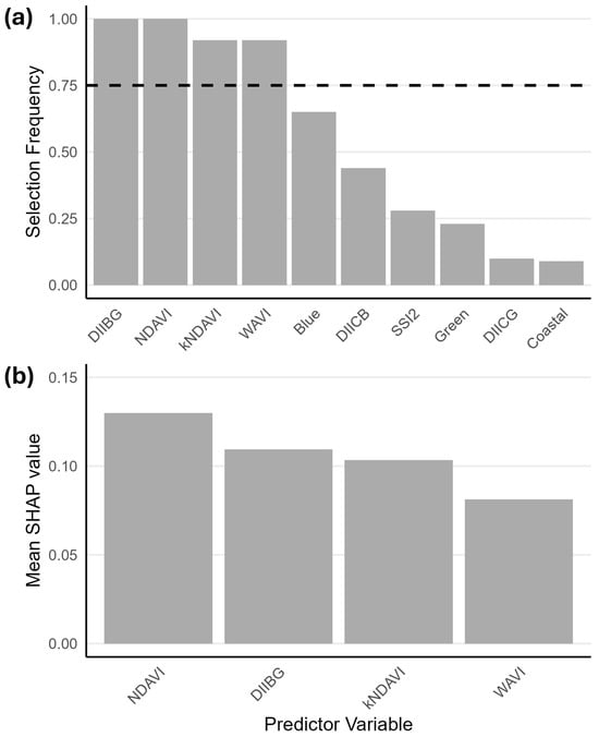
Figure 3.
(a) Selection frequency of the 10 predictor variables from 100 RF-RFE runs. The dashed line indicates the 0.75 selection frequency threshold. (b) Mean SHAP value (global importance) of each predictor variable to the model prediction of seagrass presence.
3.3. Random Forest Model Performance
Using the four selected predictor variables, the RF model performed strongly for the binary classification of seagrass versus non-seagrass habitats, achieving an overall accuracy of 0.87 and a Kappa coefficient of 0.73 (Table 3). Class-specific accuracies showed that the model classified non-seagrass more reliably than seagrass, with a producer accuracy of 0.94 for non-seagrass compared to 0.79 for seagrass (Table 3). Conversely, the user accuracy showed that the classification map was more accurate for seagrass (0.94) than for non-seagrass (0.81) (Table 3).
Table 3.
Aggregated 4-fold spatial block cross-validation results for the final RF binary classification and regression models.
For regression, which predicted continuous seagrass cover, the model performance was more modest but remained moderately strong. The coefficient of determination (R2) was 0.59, indicating that more than half of the observed variance in seagrass cover was explained by the predictors. Error metrics showed an RMSE of 15.1 and an MAE of 11.8, reflecting a notable level of uncertainty in cover estimates. Residual error was present across the full range of observed seagrass cover, with a clear pattern of systematic under-prediction at higher cover values (Figure S6).
3.4. Seagrass Distribution and Cover
Both models predicted a similar seagrass distribution within the WAEGAF area of operation (Figure 4 and Figure S7). The binary classification model predicted that 55.8% (2.31 km2) of the WAEGAF area had seagrass present (i.e., percentage cover ≥20%), whilst the regression model predicted a slightly higher presence of seagrass, 60.1% (2.49 km2) with a seagrass percentage cover ≥20% (Table 4). The abundance of seagrass in the surrounding reference area was similar but less than that predicted in the WAEGAF area for both models, with 53.1% (−2.7%) for the classification model and 53.7% (−6.4%) for the regression model (Table 4). The regression model predicted similar proportions of dense seagrass (i.e., percentage cover >40%) between the two areas, with 40.6 and 38.4% cover of dense seagrass for the WAEGAF and reference areas, respectively (Figure 4c).
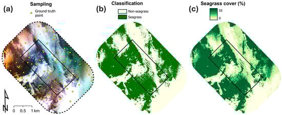
Figure 4.
WAEGAF area of operation (black rectangle) and surrounding reference area, with (a) Sentinel-2 imagery from 6 March 2025 (deep-false colour composite; histogram equalise stretch) and the 75 class-stratified ground truth sampling point locations; (b) binary classification (presence/absence) seagrass map; and (c) seagrass percentage cover map.
Table 4.
Predicted distribution and abundance of seagrass habitat in the WAEGAF area of operation and surrounding reference area.
4. Discussion
By evaluating a suite of remote sensing indices, we developed a predictive Random Forest (RF) classification model for seagrass in a moderately deep temperate embayment. The model combined two established and one emergent aquatic vegetation indices (AVIs) and the widely used Depth Invariant Index (DII) derived from Sentinel-2 blue and green bands, achieving strong performance. A complementary RF regression model, based on the same predictors, produced percentage cover estimates that were consistent with the classification outputs, although with lower overall performance. Together, these models generated spatially explicit maps of seagrass distribution and cover that provide a robust baseline and establish a workflow for cost-effective monitoring, ultimately supporting ecosystem-based fisheries management (EBFM) for the Western Australian Enhanced Greenlip Abalone Fishery and contributing to the sustainability requirements of 3rd-party stewardship certification.
Of the indices evaluated, the strongest predictors were NDAVI and DII, which are amongst the most established and widely applied indices for marine habitat assessment, reinforcing their utility. Although originally developed in shallow water environments for emergent vegetation, NDAVI has been shown to be useful for mapping seagrass and submerged aquatic vegetation (SAV) in coastal systems [20,21,24,25]. DII, developed much earlier and applied in early seagrass remote sensing studies [33], also performed strongly at this moderately deep coastal location when derived from the blue and green Sentinel-2 bands. The model accuracy improved with the inclusion of kNDAVI, showing the usefulness of this recent modification to provide complementary information to NDAVI, while WAVI, developed alongside NDAVI, also enhanced model performance in this study. In contrast, raw Sentinel-2 bands (coastal, blue, green) were infrequently selected, underscoring the superiority of derived indices over unprocessed spectral data. Similarly, DIIs incorporating the coastal band were rarely selected, likely due to the coarse native resolution (60 m) and artefact-prone nature of that band [6]. The sole seagrass-specific index included for evaluation, SSI-2, also performed poorly, offering only a moderate improvement over the raw green band from which it is derived. This is likely due to its reliance on the red band, which has limited water penetration (~7 m) [20]. The remaining seagrass-specific indices that were excluded from evaluation rely solely on the red, NIR, or SWIR bands (665–1610 nm) (Table 1), likely restricting their application to intertidal or very shallow waters (>~2.5 m depth) [20,28,31]. As such, these recently developed seagrass-specific indices are unlikely to provide significant benthic information within the study area, or the broader Western Australian temperate coast, outside of shallow estuarine environments.
Both the classification (presence/absence) and regression (percentage cover) models predicted comparable seagrass cover within the WAEGAF and surrounding reference areas, indicating a strong agreement between approaches. This consistency, together with the high accuracy of the classification model, demonstrates the utility of the methodology for rapid seagrass assessment and confirms that the two areas support similar levels of cover. However, both models predicted limited seagrass in the deeper south-eastern portion of the reference area, suggesting a potential depth threshold for seagrass occurrence at the study area. For this reason, and because of the general sloping nature of the study area (~6 to 23 m), it is important that depth be explicitly incorporated as a covariate into the design of any fine-scale seagrass monitoring programme at this location.
The classification model in this study achieved high user accuracy (0.94), indicating few false seagrass predictions but more moderate producer accuracy (0.79), meaning some seagrass areas were misclassified as non-seagrass. These conservative results, combined with the 20% cover threshold for classification of ground truth sites as seagrass, are likely to result in an underestimation of seagrass abundance and distribution, and interpretation of the presence/absence map should take this into account. The 20% cover threshold implies that sparse, ephemeral seagrass cover was unlikely to be detected in the presence/absence classification and was instead only represented in the regression model, which showed lower predictive performance. While this limitation reflects the inherent challenges of remote sensing, it is important to note that ephemeral seagrass species are typically short-lived and capable of rapid recovery following disturbance. In contrast, the moderately dense to dense perennial seagrass meadows, which are more reliably detectable in satellite imagery, represent longer-lived habitats with a greater structural persistence but slower recovery dynamics [57].
The only previous habitat map covering the study area is a broadscale map produced in 2003 in an unpublished report without available accuracy metrics [58,59]. It predicted that the WAEGAF and reference areas contained 96.8% and 93.0% “sparse ephemeral” seagrass, respectively, with the reference area also containing 0.6% “medium perennial” seagrass [59]. While variance due to seagrass seasonality, altered seagrass composition, or a decline in seagrass cover since 2003 cannot be excluded, there is no evidence to support such a shift in the habitat within the study area. A more plausible explanation is that advances in satellite technology and analytical techniques have enabled a greater mapping accuracy. Even accounting for the potential to underestimate seagrass distribution, the contrast between the predicted seagrass distribution and cover presented in this study (53–56%) and that of the previous habitat map (93–97%) underscores the need for caution when applying broadscale habitat maps for fine-scale management purposes, particularly when accuracy assessments are absent [60,61].
Several factors could present challenges for repeated remote assessments. Ground truth sampling and image capture were conducted in the late summer, when moderately deep seagrass is likely at peak abundance due to the higher light availability [57]. Future assessments should account for seasonal variability, and temporal comparisons should be made cautiously. In addition to seasonality variances, winter conditions may pose additional challenges: the elevated turbidity from adverse sea states and increased river discharge is likely to reduce light penetration and diminish the predictive capability of remote sensing indices, while the accumulation of macroalgal wrack may also be exacerbated, obscuring the benthos and potentially introducing errors and biassing seagrass estimates downward. For these reasons, we recommend that future assessments be conducted in the late summer or early autumn, coinciding with both peak seagrass abundance and periods when climate-related losses have been documented elsewhere in Western Australia [62,63].
By leveraging ready-to-use satellite products and scripted workflows in a cloud-based spatial platform, our methods are rapid, repeatable, and readily accessible to industry stakeholders. Ground truth data can be collected by a small vessel crew in less than a day with minimal post-processing, while a highly accurate trained image classifier removes the need for resource-intensive manual annotation. Together, these factors provide a cost-effective and timely approach to habitat assessment for EBFM and marine stewardship. The seagrass distribution and cover information generated here can also guide the design of fine-scale monitoring programmes by identifying suitable and representative areas of seagrass cover inside and outside the fishery area.
Numerous large-scale seagrass mortality events have been documented in Western Australia, driven by a range of stressors such as industrial and coastal development [64,65,66,67], climate-related marine heatwaves [62,63], and overgrazing [65,66,68]. These events have catalysed rehabilitation efforts [69,70,71] and highlight the need for accurate baseline mapping and cost-effective seagrass monitoring. In this study, we evaluated a suite of remote sensing indices and identified four that performed best for predicting seagrass cover in a moderately deep (6–22 m) temperate coastal embayment. Using these indices, we mapped seagrass distribution within and adjacent to the WAEGAF, providing information that supports EBFM and ongoing third-party stewardship certification. The methodology prioritises simplicity and automation, enabling rapid applications by managers or stakeholders for routine cost-effective monitoring or post-disturbance assessments, an approach that may have potential for broader applications.
5. Conclusions
This study identified a set of spectral indices derived from Sentinel-2 imagery that allowed for the detection and quantification of moderately deep (6–22 m) seagrass habitats within a temperate Western Australian embayment. When integrated into Random Forest classification and regression models, these indices produced reliable maps of seagrass distribution and cover that were consistent across the Western Australian Enhanced Greenlip Abalone Fishery area of operation and adjacent reference areas. The workflow, which combines ready-to-use satellite products, automatic image annotation, and cloud-based processing, offers a rapid, repeatable, and cost-effective method for generating habitat information critical to ecosystem-based fisheries management and third-party stewardship requirements. More broadly, this approach may provide a practical framework for aquatic resource managers to perform routine monitoring and post-disturbance assessments in other temperate coastal systems.
Supplementary Materials
The following supporting information can be downloaded at https://www.mdpi.com/article/10.3390/rs17243932/s1. Figure S1: Sentinel-2 (L2A) surface reflectance imagery of the study area from 10 February 2024 with deep-false colour composite (Bands 3,2,1) (a) prior to deglinting and (b) after deglinting; Figure S2: Line plots showing (a) the within-cluster sum of squares (WCSS) for 1–10 clusters used in the elbow method, and (b) cumulative variance explained (R2) by increasing cluster number for the unsupervised classification of Sentinel-2 imagery; Figure S3: Five-class unsupervised map of the study area with the 75 ground truth sampling points; Figure S4: A map showing an example 4-fold spatial block cross-validation with block size of 2000 m used to evaluate the final models, as well as each stability selection run for Random Forest Recursive Feature Elimination (RF-RFE); Figure S5: Grayscale composites illustrating spatial patterns in the four selected predictor variables (NDAVI, DIIBG, kNDAVI, WAVI); Figure S6: Scatterplot showing the predicted vs. observed seagrass cover from the final regression model using all 75 ground truth sampling points; Figure S7: Inset of the study area showing seagrass binary (presence/absence) ground truth points overlaid on (a) Sentinel-2 satellite imagery (deep-false colour composite) and (b) the classification model output, and (c) ground truth points of percentage cover overlaid onto the regression model output.
Author Contributions
Conceptualization, N.K., L.M., and S.N.E.; methodology, N.K., L.M., and S.N.E.; software, N.K.; validation, N.K.; formal analysis, N.K.; investigation, N.K., L.M., and S.N.E.; resources, N.K., L.M., and S.N.E.; data curation, N.K.; writing—original draft preparation, N.K.; writing—review and editing, N.K., L.M., and S.N.E.; visualisation, N.K.; project administration, N.K., L.M., and S.N.E. All authors have read and agreed to the published version of the manuscript.
Funding
This research received no external funding.
Data Availability Statement
Data available upon reasonable request to DPIRD WA (datarequest@fish.wa.gov.au), subject to confidentiality provisions and data sharing agreements.
Acknowledgments
Thanks are extended to members of the Ecological Monitoring and Assessment team within the Fisheries Research branch of DPIRD WA who assisted with the field logistics and image analysis components of the study, particularly Mitch Reid and Willow Pollard, as well as Mitch Dixon, Sam Henry, and Jithu Stephen of Rare Foods Australia for field and logistical support. We are very thankful for the three anonymous peer reviewers, as well as the DPIRD WA reviewers, for their valuable time and comments that improved the manuscript.
Conflicts of Interest
Lara Mist is a paid employee of Rare Foods Australia, a proponent of the Western Australian Enhanced Greenlip Abalone Fishery. This relationship did not influence the findings of the research.
Abbreviations
The following abbreviations are used in this manuscript:
| AIA | Automatic Image Annotation |
| AVI | Aquatic Vegetation Index |
| CATAMI | Collaborative and Automated Tools for Analysis of Marine Imagery |
| CDOM | Colour Dissolved Organic Matter |
| DEM | Digital Elevation Model |
| DII | Depth Invariant Index |
| EBFM | Ecosystem-Based Fisheries Management |
| GEE | Google Earth Engine |
| kNDAVI | Kernelised Normalised Difference Aquatic Vegetation Index |
| L2A | Sentinel-2 Level 2A |
| LiDAR | Light Detection and Ranging |
| MAE | Mean Absolute Error |
| MODIS | Moderate Resolution Imaging Spectroradiometer |
| MSI | Multispectral Instrument |
| NDAVI | Normalised Difference Aquatic Vegetation Index |
| NIR | Near-Infrared |
| RF | Random Forest |
| RF-RFE | Random Forest Recursive Feature Elimination |
| RMSE | Root Mean Squared Error |
| SAV | Submerged Aquatic Vegetation |
| SSI-2 | Seagrass Index II |
| SWIR | Shortwave Infrared |
| VIIRS | Visible Infrared Imaging Radiometer Suite |
| WAEGAF | Western Australia Enhanced Greenlip Abalone Fishery |
| WAVI | Water-Adjusted Vegetation Index |
| WCSS | Within-Cluster Sum of Squares |
References
- Townsend, H.; Harvey, C.J.; deReynier, Y.; Davis, D.; Zador, S.G.; Gaichas, S.; Weijerman, M.; Hazen, E.L.; Kaplan, I.C. Progress on Implementing Ecosystem-Based Fisheries Management in the United States Through the Use of Ecosystem Models and Analysis. Front. Mar. Sci. 2019, 6, 641. [Google Scholar] [CrossRef]
- Fletcher, W.J.; Shaw, J.; Metcalf, S.J.; Gaughan, D.J. An Ecosystem Based Fisheries Management Framework: The Efficient, Regional-Level Planning Tool for Management Agencies. Mar. Policy 2010, 34, 1226–1238. [Google Scholar] [CrossRef]
- Overly, K.E.; Lecours, V. Mapping Queen Snapper (Etelis oculatus) Suitable Habitat in Puerto Rico Using Ensemble Species Distribution Modeling. PLoS ONE 2024, 19, e0298755. [Google Scholar] [CrossRef]
- Nordlund, L.M.; Unsworth, R.K.F.; Gullström, M.; Cullen-Unsworth, L.C. Global Significance of Seagrass Fishery Activity. Fish Fish. 2018, 19, 399–412. [Google Scholar] [CrossRef]
- Menandro, P.S.; Lavagnino, A.C.; Vieira, F.V.; Boni, G.C.; Franco, T.; Bastos, A.C. The Role of Benthic Habitat Mapping for Science and Managers: A Multi-Design Approach in the Southeast Brazilian Shelf after a Major Man-Induced Disaster. Front. Mar. Sci. 2022, 9, 1004083. [Google Scholar] [CrossRef]
- Evans, S.N.; Konzewitsch, N.; Hovey, R.K.; Kendrick, G.A.; Bellchambers, L.M. Selecting the Best Habitat Mapping Technique: A Comparative Assessment for Fisheries Management in Exmouth Gulf. Front. Mar. Sci. 2025, 12, 1570277. [Google Scholar] [CrossRef]
- Davies, S.C.; Thompson, P.L.; Gomez, C.; Nephin, J.; Knudby, A.; Park, A.E.; Friesen, S.K.; Pollock, L.J.; Rubidge, E.M.; Anderson, S.C.; et al. Addressing Uncertainty When Projecting Marine Species’ Distributions under Climate Change. Ecography 2023, 2023, e06731. [Google Scholar] [CrossRef]
- Briguglio, M.; Ramírez-Monsalve, P.; Abela, G.; Armelloni, E.N. What Do People Make of “Ecosystem Based Fisheries Management”? Front. Mar. Sci. 2025, 12, 1553838. [Google Scholar] [CrossRef]
- Kachelriess, D.; Wegmann, M.; Gollock, M.; Pettorelli, N. The Application of Remote Sensing for Marine Protected Area Management. Ecol. Indic. 2014, 36, 169–177. [Google Scholar] [CrossRef]
- Li, J.; Roy, D.P. A Global Analysis of Sentinel-2a, Sentinel-2b and Landsat-8 Data Revisit Intervals and Implications for Terrestrial Monitoring. Remote Sens. 2017, 9, 902. [Google Scholar] [CrossRef]
- Copernicus Data Space Ecosystem. Sentinel-2 Level-2A. Available online: https://browser.stac.dataspace.copernicus.eu/collections/sentinel-2-l2a?.language=en (accessed on 30 September 2025).
- Phinn, S.; Roelfsema, C.; Dekker, A.; Brando, V.; Anstee, J. Mapping Seagrass Species, Cover and Biomass in Shallow Waters: An Assessment of Satellite Multi-Spectral and Airborne Hyper-Spectral Imaging Systems in Moreton Bay (Australia). Remote Sens. Environ. 2008, 112, 3413–3425. [Google Scholar] [CrossRef]
- Hossain, M.S.; Bujang, J.S.; Zakaria, M.H.; Hashim, M. The Application of Remote Sensing to Seagrass Ecosystems: An Overview and Future Research Prospects. Int. J. Remote Sens. 2015, 36, 61–114. [Google Scholar] [CrossRef]
- Traganos, D.; Reinartz, P. Mapping Mediterranean Seagrasses with Sentinel-2 Imagery. Mar. Pollut. Bull. 2018, 134, 197–209. [Google Scholar] [CrossRef]
- Gorelick, N.; Hancher, M.; Dixon, M.; Ilyushchenko, S.; Thau, D.; Moore, R. Google Earth Engine: Planetary-Scale Geospatial Analysis for Everyone. Remote Sens. Environ. 2017, 202, 18–27. [Google Scholar] [CrossRef]
- Chen, Q.; Beijbom, O.; Chan, S.; Bouwmeester, J.; Kriegman, D. A New Deep Learning Engine for CoralNet 2021. In Proceedings of the IEEE/CVF International Conference on Computer Vision, Virtual, 11–17 October 2021. [Google Scholar]
- ReefCloud. Available online: https://reefcloud.ai/ (accessed on 30 September 2025).
- Wyatt, M.; Radford, B.; Callow, N.; Bennamoun, M.; Hickey, S. Using Ensemble Methods to Improve the Robustness of Deep Learning for Image Classification in Marine Environments. Methods Ecol. Evol. 2022, 13, 1317–1328. [Google Scholar] [CrossRef]
- Evans, S.N.; Philippa, B.; Mattone, C.; Konzewitsch, N.; Hovey, R.K.; Sheaves, M.; Kendrick, G.A.; Bellchambers, L.M. Advancing Fishery Dependent and Independent Habitat Assessments Using Automated Image Analysis: A Fisheries Management Agency Case Study. PLoS ONE 2025, 20, e0329409. [Google Scholar] [CrossRef] [PubMed]
- Bannari, A.; Ali, T.S.; Abahussain, A. The Capabilities of Sentinel-MSI (2A/2B) and Landsat-OLI (8/9) in Seagrass and Algae Species Differentiation Using Spectral Reflectance. Ocean Sci. 2022, 18, 361–388. [Google Scholar] [CrossRef]
- Villa, P.; Mousivand, A.; Bresciani, M. Aquatic Vegetation Indices Assessment through Radiative Transfer Modeling and Linear Mixture Simulation. Int. J. Appl. Earth Obs. Geoinf. 2014, 30, 113–127. [Google Scholar] [CrossRef]
- Alkhatlan, A.; Bannari, A.; El-Battay, A.; Al-Dawood, T.; Abahussain, A. Potential of Landsat-OLI for Seagrass and Algae Species Detection and Discrimination in Bahrain National Water Using Spectral Reflectance. In Proceedings of the International Geoscience and Remote Sensing Symposium (IGARSS), Valencia, Spain, 22–27 July 2018; Institute of Electrical and Electronics Engineers Inc.: Piscataway, NJ, USA; pp. 4043–4046. [Google Scholar]
- Moeen, M.; Babin, D.; Tentoglou, T.; Waite, T.; Young, K. NASA Technical Reports Server (NTRS). In Louisiana Water Resources: Using NASA Earth Observations to Monitor Historical Changes in the Extension of Seagrass Meadows in the Breton National Wildlife Refuge in Louisiana; NASA Develop National Program; National Aeronautics and Space Administration: Washington, DC, USA, 2021. [Google Scholar]
- Deeks, E.; Magalhães, K.; Traganos, D.; Ward, R.; Normande, I.; Dawson, T.P.; Kratina, P. Seagrass Mapping of North-Eastern Brazil Using Google Earth Engine and Sentinel-2 Imagery. Environ. Sustain. Indic. 2024, 24, 100489. [Google Scholar] [CrossRef]
- Mastrantonis, S.; Radford, B.; Langlois, T.; Spencer, C.; de Lestang, S.; Hickey, S. A Novel Method for Robust Marine Habitat Mapping Using a Kernelised Aquatic Vegetation Index. ISPRS J. Photogramm. Remote Sens. 2024, 209, 472–480. [Google Scholar] [CrossRef]
- Wang, Q.; Moreno-Martínez, Á.; Muñoz-Marí, J.; Campos-Taberner, M.; Camps-Valls, G. Estimation of Vegetation Traits with Kernel NDVI. ISPRS J. Photogramm. Remote Sens. 2023, 195, 408–417. [Google Scholar] [CrossRef]
- Li, Y.; Bai, J.; Chen, S.; Chen, B.; Zhang, L. Mapping Seagrasses on the Basis of Sentinel-2 Images under Tidal Change. Mar. Environ. Res. 2023, 185, 105880. [Google Scholar] [CrossRef]
- Liang, H.; Wang, L.; Wang, S.; Sun, D.; Li, J.; Xu, Y.; Zhang, H. Remote Sensing Detection of Seagrass Distribution in a Marine Lagoon (Swan Lake), China. Opt. Express 2023, 31, 27677. [Google Scholar] [CrossRef]
- Bai, J.; Li, Y.; Chen, S.; Du, J.; Wang, D. Long-Time Monitoring of Seagrass Beds on the East Coast of Hainan Island Based on Remote Sensing Images. Ecol. Indic. 2023, 157, 111272. [Google Scholar] [CrossRef]
- Lobell, D.B.; Asner, G.P. Hyperion Studies of Crop Stress in Mexico. In Proceedings of the 12th JPL Airborne Earth Science Workshop, Pasadena, CA, USA, 31 March 2004. [Google Scholar]
- Komatsu, T.; Hashim, M.; Nurdin, N.; Noiraksar, T.; Prathep, A.; Stankovic, M.; Phuoc, T.; Son, H.; Thu, M.; Van Luong, C.; et al. Practical Mapping Methods of Seagrass Beds by Satellite Remote Sensing and Ground Truthing. Coast. Mar. Sci. 2020, 43, 1–25. [Google Scholar]
- Green, E.P.; Mumby, P.J.; Edwards, A.J.; Clark, C.D. Remote Sensing Handbook for Tropical Coastal Management; Edwards, A.J., Ed.; UNESCO: Paris, France, 2000. [Google Scholar]
- Mumby, P.J.; Green, E.P.; Edwards, A.J.; Clark, C.D. Measurement of Seagrass Standing Crop Using Satellite and Digital Airborne Remote Sensing. Mar. Ecol. Prog. Ser. 1997, 159, 51–60. [Google Scholar] [CrossRef]
- Lyzenga, D.R. Passive Remote Sensing Techniques for Mapping Water Depth and Bottom Features. Appl. Opt. 1978, 17, 379. [Google Scholar] [CrossRef] [PubMed]
- Rowan, G.S.L.; Kalacska, M. A Review of Remote Sensing of Submerged Aquatic Vegetation for Non-Specialists. Remote Sens. 2021, 13, 623. [Google Scholar] [CrossRef]
- Chin, A.; Conci, M.; Treptow, A.; Markell, G. Assessing Recreational Fish Habitats in Florida Using Earth Observations; Develop Technical Report; Coastal Florida Ecological Conservation. In Proceedings of the 8th International Science Symposium, Fort Lauderdale, FL, USA, 7–8 November 2025. [Google Scholar]
- Andskog, M.A.; Layman, C.; Allgeier, J.E. Seagrass Production around Artificial Reefs Is Resistant to Human Stressors. Proc. R. Soc. B Biol. Sci. 2023, 290, 20230803. [Google Scholar] [CrossRef] [PubMed]
- Ocean Grown Abalone Pty. Ltd. Aquaculture Management and Environmental Monitoring Plan (MEMP); Ocean Grown Abalone Ltd.: Augusta, Australia, 2020. [Google Scholar]
- Waycott, M.; Duarte, C.M.; Carruthers, T.J.B.; Orth, R.J.; Dennison, W.C.; Olyarnik, S.; Calladine, A.; Fourqurean, J.W.; Heck, K.L.; Hughes, A.R.; et al. Accelerating Loss of Seagrasses across the Globe Threatens Coastal Ecosystems. Proc. Natl. Acad. Sci. USA 2009, 106, 12377–12381. [Google Scholar] [CrossRef]
- WA Department of Transport. Donnelly_20230410_Cape_Leeuwin_Augusta_LiDAR. Available online: https://www.arcgis.com/apps/webappviewer/index.html?id=d58dd77d85654783b5fc8c775953c69b (accessed on 2 September 2025).
- Hedley, J.D.; Harborne, A.R.; Mumby, P.J. Simple and Robust Removal of Sun Glint for Mapping Shallow-Water Benthos. Int. J. Remote Sens. 2005, 26, 2107–2112. [Google Scholar] [CrossRef]
- Wickham, H.; Averick, M.; Bryan, J.; Chang, W.; McGowan, L.; François, R.; Grolemund, G.; Hayes, A.; Henry, L.; Hester, J.; et al. Welcome to the Tidyverse. J. Open Source Softw. 2019, 4, 1686. [Google Scholar] [CrossRef]
- Pebesma, E. Simple Features for R: Standardized Support for Spatial Vector Data. 2018. [Google Scholar]
- Robert, M.; Hijmans, J. Package “terra” Type Package Title Spatial Data Analysis; R Foundation for Statistical Computing: Vienna, Austria, 2025. [Google Scholar]
- Althaus, F.; Hill, N.; Ferrari, R.; Edwards, L.; Przeslawski, R.; Schönberg, C.H.L.; Stuart-Smith, R.; Barrett, N.; Edgar, G.; Colquhoun, J.; et al. A Standardised Vocabulary for Identifying Benthic Biota and Substrata from Underwater Imagery: The CATAMI Classification Scheme. PLoS ONE 2015, 10, e0141039. [Google Scholar] [CrossRef]
- Zhou, Q.; Ke, Y.; Wang, X.; Bai, J.; Zhou, D.; Li, X. Developing seagrass index for long term monitoring of Zostera japonica seagrass bed: A case study in Yellow River Delta, China. ISPRS J. Photogramm. Remote Sens. 2022, 194, 286–301. [Google Scholar] [CrossRef]
- Poursanidis, D.; Katsanevakis, S. Mapping Subtidal Marine Forests in the Mediterranean Sea Using Copernicus Contributing Mission. Remote Sens. 2025, 17, 2398. [Google Scholar] [CrossRef]
- Hu, W.; Zhang, D.; Chen, B.; Liu, X.; Ye, X.; Jiang, Q.; Zheng, X.; Du, J.; Chen, S. Mapping the Seagrass Conservation and Restoration Priorities: Coupling Habitat Suitability and Anthropogenic Pressures. Ecol. Indic. 2021, 129, 107960. [Google Scholar] [CrossRef]
- Meinshausen, N.; Bühlmann, P. Stability Selection. J. R. Stat. Soc. Ser. B Stat. Methodol. 2010, 72, 417–473. [Google Scholar] [CrossRef]
- Kuhn, M. Building Predictive Models in R Using the Caret Package. J. Stat. Softw. 2008, 28, 1–26. [Google Scholar] [CrossRef]
- Wickham, H. Ggplot2. WIREs Comput. Stat. 2011, 3, 180–185. [Google Scholar] [CrossRef]
- Liaw, A.; Weiner, M. Classification and Regression by RandomForest. R News 2002, 2, 18–22. [Google Scholar]
- R Core Team. R: A Language and Environment for Statistical Computing; R Foundation for Statistical Computing: Vienna, Austria, 2025. [Google Scholar]
- Valavi, R.; Elith, J.; Lahoz-Monfort, J.J.; Guillera-Arroita, G. blockCV: An r package for generating spatially or environmentally separated folds for k-fold cross-validation of species distribution models. Methods Ecol. Evol. 2019, 10, 225–232. [Google Scholar] [CrossRef]
- Jethani, N.; Sudarshan, M.; Covert, I.; Lee, S.I.; Ranganath, R. Fastshap: Real-time shapley value estimation. ICLR 2022, 2022. [Google Scholar] [CrossRef]
- Google Earth Engine. Ee.Classifier.SmileRandomForest. Available online: https://developers.google.com/earth-engine/apidocs/ee-classifier-smilerandomforest (accessed on 25 September 2025).
- Kilminster, K.; McMahon, K.; Waycott, M.; Kendrick, G.A.; Scanes, P.; McKenzie, L.; O’Brien, K.R.; Lyons, M.; Ferguson, A.; Maxwell, P.; et al. Unravelling Complexity in Seagrass Systems for Management: Australia as a Microcosm. Sci. Total Environ. 2015, 534, 97–109. [Google Scholar] [CrossRef]
- Bancroft, K.P. A Standardised Classification Scheme for the Mapping of Shallow-Water Marine Habitats in Western Australia. Report MCB-05/2003. Unpublished work. 2002. [Google Scholar]
- Department of Parks and Wildlife, Western Australian Government, Marine Habitats of Western Australia. Available online: https://researchdata.edu.au/marine-habitats-western-australia/967012 (accessed on 10 October 2025).
- Ware, S.; Downie, A.L. Challenges of Habitat Mapping to Inform Marine Protected Area (MPA) Designation and Monitoring: An Operational Perspective. Mar. Policy 2020, 111, 103717. [Google Scholar] [CrossRef]
- Strong, J.A. An Error Analysis of Marine Habitat Mapping Methods and Prioritised Work Packages Required to Reduce Errors and Improve Consistency. Estuar. Coast. Shelf Sci. 2020, 240, 106684. [Google Scholar] [CrossRef]
- Kendrick, G.A.; Nowicki, R.; Olsen, Y.S.; Strydom, S.; Fraser, M.W.; Sinclair, E.A.; Statton, J.; Hovey, R.K.; Thomson, J.A.; Burkholder, D.; et al. A Systematic Review of How Multiple Stressors from an Extreme Event Drove Ecosystem-Wide Loss of Resilience in an Iconic Seagrass Community. Front. Mar. Sci. 2019, 6, 455. [Google Scholar] [CrossRef]
- Strydom, S.; Murray, K.; Wilson, S.; Huntley, B.; Rule, M.; Heithaus, M.; Bessey, C.; Kendrick, G.A.; Burkholder, D.; Fraser, M.W.; et al. Too Hot to Handle: Unprecedented Seagrass Death Driven by Marine Heatwave in a World Heritage Area. Glob. Chang. Biol. 2020, 26, 3525–3538. [Google Scholar] [CrossRef]
- Cambridge, M.L.; Mccomb, A.J. The loss of seagrasses in Cockburn Sound, Western Australia. I. The time course and magnitude of seagrass decline in relation to industrial development. Aquat. Bot. 1984, 20, 229–243. [Google Scholar]
- Kendrick, G.A.; Aylward, M.J.; Hegge, B.J.; Cambridge, M.L.; Hillman, K.; Wyllie, A.; Lord, D.A. Changes in Seagrass Coverage in Cockburn Sound, Western Australia between 1967 and 1999. Aquat. Bot. 2002, 1, 75–87. [Google Scholar] [CrossRef]
- Buckee, J.; Hetzel, Y.; Nyegaard, M.; Evans, S.; Whiting, S.; Scott, S.; Ayvazian, S.; van Keulen, M.; Verduin, J. Catastrophic Loss of Tropical Seagrass Habitats at the Cocos (Keeling) Islands Due to Multiple Stressors. Mar. Pollut. Bull. 2021, 170, 112602. [Google Scholar] [CrossRef]
- Walker, D.I.; Mccomb, A.J. Seagrass Degradation in Australian Coastal Waters. Mar. Poll. Bull. 1992, 25, 191–195. [Google Scholar] [CrossRef]
- Konzewitsch, N.; Evans, S.N. Time-Series Satellite Image Classification Reveals Comprehensive Canopy Loss of Dense Thalassodendron Ciliatum Seagrass Meadows at Cocos (Keeling) Islands. Mar. Biol. 2024, 171, 45. [Google Scholar] [CrossRef]
- Sinclair, E.A.; Statton, J.; Austin, R.; Breed, M.F.; Cross, R.; Dodd, A.; Kendrick, A.; Krauss, S.L.; McNeair, B.; McNeair, N.; et al. Healing Country Together: A Seagrass Restoration Case Study from Gathaagudu (Shark Bay). Ocean Coast. Manag. 2024, 256, 107274. [Google Scholar] [CrossRef]
- Kendrick, G.A.; Austin, R.; Ferretto, G.; van Keulen, M.; Verduin, J.J. Lessons Learnt from Revisiting Decades of Seagrass Restoration Projects in Cockburn Sound, Southwestern Australia. Restor. Ecol. 2025, 33, e70040. [Google Scholar] [CrossRef]
- Sinclair, E.A.; Sherman, C.D.; Statton, J.; Copeland, C.; Matthews, A.; Waycott, M.; van Dijk, K.J.; Vergés, A.; Kajlich, L.; McLeod, I.M.; et al. Advances in Approaches to Seagrass Restoration in Australia. Ecol. Manag. Restor. 2021, 22, 10–21. [Google Scholar] [CrossRef]
Disclaimer/Publisher’s Note: The statements, opinions and data contained in all publications are solely those of the individual author(s) and contributor(s) and not of MDPI and/or the editor(s). MDPI and/or the editor(s) disclaim responsibility for any injury to people or property resulting from any ideas, methods, instructions or products referred to in the content. |
© 2025 by the authors. Licensee MDPI, Basel, Switzerland. This article is an open access article distributed under the terms and conditions of the Creative Commons Attribution (CC BY) license (https://creativecommons.org/licenses/by/4.0/).