Modeling BRDF over Row Crops Canopy with Effects of Intra-Row Heterogeneity

Highlights

What are the main findings?

• A new model for row crops is proposed by introducing three control parameters, effectively capturing the high spatial intra-row heterogeneity and simulating dynamic evolution across the life cycle, leading to a more realistic structural representation.
• The new model demonstrates high accuracy in simulating the BRDF for the row crops canopy, with the three control parameters playing a critical role in shaping reflectance in the darkspot direction.

What are the implications of the main findings?

• The model provides reliable support for remote sensing parameter retrieval and digital twin applications in agricultural fields, improving the accuracy of crop monitoring and yield estimation.
• The new model establishes a unified framework for row crops, which bridges the row structure and continuous canopy stages.

Abstract

Row crops are regarded as a transitional type between continuous and discrete vegetation. Previous studies idealized row crops as periodic hedgerows with rectangular cross-sections. However, these models relied on oversimplified assumptions, failing to capture the intrinsic heterogeneity of canopy or its dynamic evolution over the life cycle. In 2020, we proposed a row crop model with a gradual decrease in leaf area volume density (LAVD) from the center of the row to the edge, partially overcoming these limitations. Building on this previous model, this paper introduces the leaf shape factor proposed by Mõttus et al. into the model. Three control parameters, a leaf width control parameter (β), leaf length control parameter (ψ), and leaf azimuth control parameter (e), are proposed to regulate the spatial distribution of LAVD. Additionally, an empirical exponential function from Watanabe et al. is adopted to describe the leaf zenith angle distribution, enabling the realistic calculation of the G-function and Γ-function in conjunction with leaf azimuth distribution. The LAVD is formulated at three hierarchical scales: individual scale, row scale, and scene scale. The model delivers two key advancements: enabling pronounced spatial heterogeneity and high tunability of the LAVD, and accurately simulating row crops throughout the life cycle, which bridges the row structure and continuous stages of row crops. Radiative transfer simulations are conducted to derive the bidirectional reflectance distribution function (BRDF), which is validated against the discrete anisotropic radiative transfer (DART) model. Comparisons across three growth stages demonstrated good consistency. Furthermore, this paper investigates the sensitivity of the BRDF to three control parameters (β, ψ, and e). The results indicate that changes in three parameters significantly affect the reflectance in the darkspot direction, leading to a maximum error of 22.6%. In carrying out remote sensing applications such as parameter inversion and yield estimation for row crops, the new model is recommended for more accurate BRDF simulations.

1. Introduction

Row crops, a significant category of terrestrial vegetation, are extensively distributed across the world. Due to row planting, the canopy structure of row crops exhibits distinct characteristics compared to naturally formed vegetation. For a considerable time during the early and middle part of the growing season, the canopy of row crops is composed of laterally alternating strips of vegetation and bare soil. This asymmetric distribution results in significant directional anisotropy in the reflectance of row crops [1,2,3]. In the late stage of the growing season, the canopy transforms into a more homogeneous structure after canopy closure [4,5]. The bidirectional reflectance distribution function (BRDF) of the row crop canopy contains crucial ecological parameters of cropland, such as leaf area index (LAI), fractional vegetation cover (FVC), canopy height, row width, and chlorophyll content, which are essential for monitoring crop growth and estimating yield [6,7,8]. Therefore, establishing an accurate BRDF model for row crops is fundamental for improving the retrieval accuracy of farmland ecological parameters, and further estimating absorbed photosynthetically active radiation (FAPAR) and parameters of the carbon cycle [9].

The canopy of row crops is regarded as a transitional type between continuous and discrete vegetation [2], exhibiting distinct heterogeneity: discrete in the cross-row direction and continuous in the along-row direction, therefore inducing a unique bidirectional reflectance pattern referred to as the row effect. Considerable research efforts have been devoted to the modeling of row crops and their BRDF. As early as 1972, Jackson et al. [10] demonstrated through experiments and simulations that neglecting row architecture induces significant reflectance bias for the row crop canopy. Subsequent work by Jackson et al. [3] and later Kimes et al. [11] abstracted row crops as an extended rectangular solid without gaps and calculated the proportions of four components (sunlit vegetation, sunlit soil, shaded soil, and shaded vegetation) of the projected area in the viewing direction. This established the Kimes model as a pioneer in BRDF modeling of row crops. However, Kimes neglected gaps within the row structure. To address this problem, Chen et al. [12] introduced Li’s discrete canopy gap model [13] and Kuusk’s bidirectional gap model [14] into the Kimes model. Meanwhile, Yan et al. [15] introduced Li’s gap model [13] and Jupp’s bidirectional gap theory [16] into the Kimes model. Yan et al. [2] and Peng et al. [17] regarded the canopy of row crops as a result of leaf aggregation at the canopy scale and adopted a clumping index [18] to describe this heterogeneity, linking row crops with continuous vegetation. However, Yan et al. derived the clumping index exclusively for the homogeneous row structure, leaving the clumping index of the heterogeneous row structure unresolved. Afterwards, Yu et al. extended the clumping index to the thermal infrared band to simulate the brightness temperature of the maize canopy in the row structure [19].

All aforementioned models for row crops are categorized as the geometric optical (GO) model. The GO model precisely characterizes the geometric attributes of the canopy, making it ideal for the heterogeneous canopy [20]. The canopy of row crops exhibits distinct geometric features (e.g., canopy height, row width, and intra-row spacing), and the GO model excels at capturing these structural patterns. Consequently, the GO model has been extensively applied in the modeling of row crops [21,22,23]. While the GO model achieves accurate BRDF simulations in the visible spectrum, it systematically underestimates BRDF in the near-infrared (NIR) band due to unaccounted multiple scattering [24]. To date, extensive efforts have been dedicated to modeling multiple scattering within the GO model. Li et al. [25] developed a hybrid geometric optical-radiative transfer approach (GORT) by introducing the radiative transfer (RT) approach to estimate the multiple-scattering contribution. Chen et al. [24] introduced viewing factors between illuminated and shaded components to compute multiple scattering. Ma et al. [22] implemented the adding method [26,27] for multiple-scattering calculations in row crops. For the RT model, Suits et al. [28] introduced density modulation on the basis of the uniform canopy reflectance model [29]. Suits believed that density modulation is the evidence for the existence of row structure and is the measure of the amount of row structure. The density was considered to be large in the center of the row and gradually decreased to zero between rows depending upon the lateral displacement from the row centers. The modulation was considered to be the same for all canopy layers. Zhou et al. [30] developed a 4SAIL-RowCrop model for row crops by integrating the 4SAIL model [31] and the Kimes model. Wang et al. [32] developed a multiple-layer canopy reflectance model (MRTM) focusing on the effect of canopy vertical heterogeneity on the reflectance. Afterwards, Zhao et al. [33] extended the MRTM to the crops. Zhou et al. [5] developed an aquatic vegetation row model (AVRM), taking into account the water background for row crops.

Current models for row crops inadequately address canopy heterogeneity, typically accounting for only horizontal or vertical heterogeneity. However, row crops exhibit significant spatial heterogeneity in both dimensions simultaneously. Moreover, the growth of crops is a continuous process, during which the canopy undergoes a dynamical transition from a distinct row structure to continuous vegetation. A common modeling strategy is to treat row crops as a discrete row structure before canopy closure and as continuous vegetation afterward, with separate models applied to each stage. This modeling method introduces an artificial discontinuity, hindering the establishment of a unified model across the life cycle for row crops. In conclusion, a unified model for row crops capable of capturing high spatial heterogeneity throughout the entire life cycle is critically needed.

Du et al. (2007) first introduced an ideal single plant as the foundational component for crop scene modeling and DBT (directional brightness temperature) simulation. Building on this concept, they developed the SLEC (soil leaf ear combined) model for mature crops at the ear stage [34]. Subsequently, the approach was extended to simulate a row crop canopy across the entire life cycle [35]. Du et al. [34] regarded the row crops as the periodic permutation of the row structure by treating the row structure as the random permutation of an individual plant, and thus constructed an elaborate model of row crops. Du et al. believed that the density of leaves in the row reaches a maximum in the row center, and decreases gradually with the distance from the center. For a single plant, LAVD is high at the center of an individual plant and decreases gradually with the distance from the stem of the plant in a centrosymmetric manner. On these bases, LAVD was formulated at an individual scale, row scale, and scene scale hierarchically. The model performed well throughout the growth cycle of row crops. At present, this model is only applicable in the thermal infrared, but it also serves a purpose in modeling BRDF in the visible and near-infrared (V-NIR) band. In this study, we further improve the row crop model proposed by Du et al. [34] to better simulate the heterogeneity of the row crop canopy throughout the entire life cycle and apply it on the BRDF simulation of row crop canopy.

2. Materials and Methods

2.1. Modeling Leaf Area Volume Density Distribution (LAVD) on an Individual Scale

For the convenience of discussion, a Cartesian coordinate system is introduced at the scene scale (Figure 1a), and a cylindrical coordinate system is introduced at the individual scale (Figure 1b). According to Du et al. [35], the LAVD spatial distribution at the individual scale is calculated as follows.

$$Di\left(\rho ,\phi ,z\right)={\displaystyle \frac{nw}{2\pi \rho \mu H}}$$

(1)

where ρ is the distance from the stem, φ is the azimuth, z is the height, n is the number of leaves inserted on a single stem, w is the leaf width, H is the height of the canopy, and µ is the cosine of the leaf zenith angle.

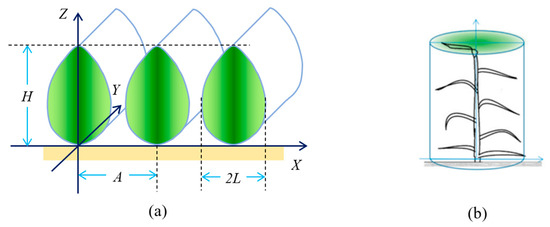
Figure 1. Coordinate system for row crop scene and for individual plants. (a) The Cartesian coordinate system for the row structure. A is the distance between two neighboring row centers, L is the half-width of a row structure; H is the height of row structure. (b) The cylindrical coordinate system for the individual scale.

The LAVD equation described above relies on three fundamental assumptions: (1) each leaf is a long and narrow rectangle; (2) leaf azimuth angles follow a uniform distribution; and (3) leaf vertical distribution is uniform. However, these simplifications diverge from observed canopy architectures, where leaves exhibit an irregular figure and curvature, preferential azimuthal orientations, and stratified vertical arrangements. To bridge these gaps, three control parameters are introduced to enhance the model’s heterogeneity, flexibility, and applicability.

(1)

Leaf width control parameter (β)

The geometric architecture of the canopy predominantly governs radiative transfer processes. Significant research efforts have been dedicated to modeling vegetation geometric structures, including Mõttus’ work on heterogeneous canopies. Mõttus proposed an analytical leaf shape function for narrow leaves [36], simulated the fractional areas of sunflecks, penumbra, and umbra within the coppice canopy [37], estimated the crown volume of trees [38], calculated the recollision probability in heterogeneous forest canopies [39,40], presented an open dataset for multitask learning of continuous and categorical forest variables from hyperspectral imagery (TAIGA, artificial intelligence dataset for forest geographical applications) [41], and investigated the seasonal and vertical effects of canopy structure on canopy reflectance in a rice field [42]. Mõttus et al. highlight that leaf shape significantly influences radiative transfer processes [36]. However, current models focus exclusively on canopy-scale geometric structures, treating the canopy interiors as a turbid medium and overlooking leaf shape complexity. Real leaf shapes in a canopy are intricate and variable. Comprehensively measuring the leaves in a canopy is impractical. Therefore, leaf shape descriptions for radiative transfer models must not only closely match actual measurements but also be robust [36]. For this aim, Mõttus et al. [36] proposed an analytical shape function for a narrow simple leaf whose shape cannot be modeled by simple geometrical figures. The function describes the leaf half-width at point x on the midrib

$$f_L\left(x,l,w,\beta \right)={\displaystyle \frac{w}{2}}\left(1-\beta {\displaystyle \frac{x}{l}}\right){\left({\displaystyle \frac{x}{l}}-{\left({\displaystyle \frac{x}{l}}\right)}^2\right)}^{\beta }v\left(\beta \right),0\le x\le l,0\le \beta \le 1$$

(2)

$$v\left(\beta \right)={\displaystyle \frac{2^{1+\beta }{\left(1+2\beta \right)}^{1+2\beta }}{\left(2+\beta -{\beta }^2+\beta u\left(\beta \right)\right){\left({\beta }^2+5\beta -4+\left(2-\beta \right)u\left(\beta \right)\right)}^{\beta }}}$$

(3)

$$u\left(\beta \right)=\sqrt{5-2\beta +{\beta }^2}$$

(4)

where l and w are the length and maximum width of a leaf, respectively. The parameter β (0 ≤ β ≤ 1) is a hyperparameter characterizing leaf shape. Leaf shape at different values of β with constant l and w are illustrated in Figure 2c. At β = 0, the leaf appears as a rectangle. As β increases, the leaf shape shrinks to a drop shape. At β = 1, the shape function f_L is a third-order polynomial. According to Equation (1), the leaf width affects the LAVD directly. The leaf shape function approximates the contour of the real leaf closely and gives the possibility of computing the leaf area, while preserving the natural variability of leaf shape through the parameter β.

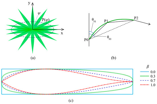
Figure 2. Leaf azimuth distribution, zenith, and shape. (a) Top-view sketch of leaf occurrence probability. (b) The curve of the leaf midrib: P1 is the midpoint of the leaf, and P1 and P2 are the endpoints of the leaf. (c) Leaf shape at different values of β (l and w are constant).

(2)

Leaf azimuth control parameter (e)

Previous studies have mainly focused on the zenith angle of leaves while assuming a random leaf azimuth distribution [43,44,45]. This assumption remains valid for natural ecosystems such as forests but fails for row crops [46,47,48]. When crops are planted in rows, leaves tend to be lateral due to adiation interception, competition for water and nutrients, and other reasons [49,50], which means that the azimuth angles of leaves are heterogeneous. To describe this phenomenon, the leaf azimuth distribution probability density function is modeled using an ellipse, whose eccentricity serves as the control parameter for the azimuth distribution (Figure 2a). The minor axis of the ellipse is coaxial with row direction, whereas the major axis extends orthogonally to row direction. The azimuth starts from the positive y-axis (row direction), with positive angular increments following a clockwise direction. The leaf occurrence probability varies with azimuth (ψ) as follows

$$P\left(\phi ,e\right)={\displaystyle \frac{\sqrt{1-e^2}}{\sqrt{1-{\left(e·sin\left(\phi \right)\right)}^2}}}$$

(5)

The larger the elliptical eccentricity, the closer the leaf is to a plane perpendicular to the row direction. If the ellipse degenerates into a circle, the leaf has the same probability of appearing at all azimuths. Under maximum eccentricity (e = 1), the ellipse degenerates to a line, thus all leaves grow perpendicular to the row direction. In this configuration, canopy light interception is minimized, which also serves as an indicator of water deficit for row crops [49]. Additionally, Equation (5) needs to be normalized over the entire 2π azimuthal domain.

(3)

Leaf length control parameter (ψ)

There have been increasing works focusing on the effects of vertical heterogeneity of the canopy structure [32,33,42,51]. Leaf length varies with the height [48]. To capture this height-dependent variation, we implement the same analytical shape function [36] with control parameter ψ. The range of ψ is extended to [−1, 1]. The leaf horizontal length at height z is

$$l\left(z,\psi \right)=\left\{\begin{array}{cc}{f}_L\left(h,H,2L,\psi \right),\hfill & \psi \ge 0\\ f_L\left(H-h,H,2L,\left|\psi \right|\right),\hfill & \psi <0\end{array}\right.$$

(6)

where H represents the canopy height, L is the half-width of the row structure and is also the horizontal length of the longest leaf in the canopy. Consequently, ψ < 0 produces an upright drop shape for the canopy envelope with a longer leaf on the top; ψ > 0 yields an inverted drop shape for the canopy envelope with a longer leaf on the bottom; and ψ = 0 results in a rectangular canopy. The leaf length control parameter (ψ) determines the shape of a single plant and the envelope of a row structure (Figure 3).

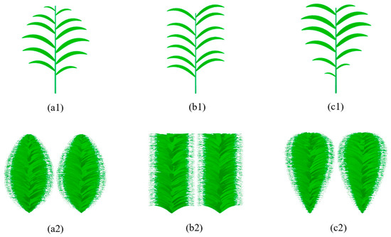
Figure 3. The single plant and envelope of the row structure for different ψ. (a1), (b1), and (c1) represent a single plant for ψ = 0.5, 0.0, −0.5, respectively. (a2), (b2), (c2) represent the envelope of the row structure for ψ = 0.5, 0.0, −0.5, respectively. A = 0.8 m, L = 0.4 m, H = 1.2 m, and θ₀₁ = 45°.

(4)

Leaf midrib curve

The above analytical leaf shape function describes the shape of flat leaves. However, due to forces and other factors, leaves are curved, exhibiting spatial heterogeneity in leaf zenith angles. The empirical exponential function proposed by Watanabe et al. [52] is adopted to calculate the zenith of the midrib

$${\theta }_{03}=81.7\left(1-\exp \left(-0.0379{\theta }_{01}\right)\right)$$

(7)

The leaf midrib curve is shown in Figure 2b. It is assumed to be quadratic and can be solved. Afterwards, the zenith angle is derived and denoted as θ(ρ,l), where l is the horizontal length of the leaf. The leaf inclination at the individual scale is

$${\mathsf{\Omega }}_L\left(\rho ,\phi ,z\right)=\left[\theta \right(\rho ,l\left(z,\psi \right)),\phi ]$$

(8)

(5)

The LAVD at individual scale

Incorporating the aforementioned refinements in leaf dimensions (width and length) and orientations (azimuth and zenith angles), LAVD spatial distribution at the individual scale is modified as

$$Di\left(\rho ,\phi ,z\right)={\displaystyle \frac{n·f_L\left(\rho ,l\left(z\right),l\left(z\right)·\alpha \right)·P\left(\phi \right)}{2\pi \rho H·\cos (\theta (\rho ,l\left(z\right)\left)\right)}}$$

(9)

where α is the ratio of leaf width to length. Both n and α are constant intermediate variables that require no configuration and can be substituted by LAI. Parameters β, ψ, and e are hyperparameters and thus omitted from Equation (9), as well as subsequent equations.

(6)

The LAVD at row scale

Once the LAVD at the individual scale is defined, the LAVD at the row scale can be obtained by integrating the Di values for all individuals whose leaves can reach the given point (Figure 4). Crops are usually planted in line uniformly. The LAVD parallel to the row direction can be assumed to be homogeneous. In contrast, the LAVD across the row direction is highly heterogeneous. Thus, the representation of LAVD spatial distribution is simplified from three-dimensional to two-dimensional. LAVD spatial heterogeneity only needs to be considered in the cross-row plane. The LAVD at row scale is calculated as

$$Dr\left(x,z\right)={\int }_{-y_o}^{y_o}Di\left(\rho ,\phi ,z\right)\mathrm{d}y$$

(10)

$$y_o=\sqrt{{l\left(z\right)}^2-x^2}$$

(11)

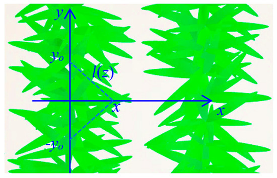
Figure 4. The top view of a row crop canopy and the integral range for the leaf area volume density (LAVD) at the row scale.

The integral range diminishes with increasing distance from the row centerline, while the LAVD at the individual scale decreases radially. Consequently, the horizontal heterogeneity of LAVD arises from the coupling of these two spatial trends. The vertical heterogeneity of LAVD is driven solely by the variations in leaf length.

(7)

The LAVD at scene scale

Given the periodic nature of the row structure, the scene-scale LAVD is obtained by summing the row-scale LAVD of adjacent rows.

$$D(x,z)=Dr(x,z)+Dr(A-x,z)$$

(12)

2.2. G-Function

G is defined as the mean projection of unit foliage area, and is a function of the transmission direction in a certain canopy [53,54]. The G-function characterizes the probability of radiation interacting with the leaves and is a fundamental quantity that plays a critical role in modeling radiative transfer within vegetation canopies. In previous studies, the leaf inclination distribution function (LIDF) in the canopy was not available and was assumed to be a spherical distribution, namely G ≡ 0.5. However, this hypothesis holds true near the zenith angle of 57.5°, and causes significant deviations at other zenith angles [55]. Compared to existing models, the new model provides a detailed characterization of LAVD and LIDF, establishing the calculation for the spatial distribution of G.

$$G\left(x,z,\mathsf{\Omega }\right)={\displaystyle \frac{{\int }_{-y_o}^{y_o}Di\left(\rho ,\phi ,z\right)·\left|{\mathsf{\Omega }}_L\left(\rho ,\phi ,z\right)·\mathsf{\Omega }\right|\mathrm{ d}y}{{\int }_{-y_o}^{y_o}Di\left(\rho ,\phi ,z\right)\mathrm{d}y}}$$

(13)

2.3. Γ-Function

Γ is the scattering phase function of the canopy medium [54,56]. In the same way as G, Γ determines the interception and scattering of light. According to its physical definition, it is calculated as

$$\Gamma \left(x,z,{\mathsf{\Omega }}_{in},{\mathsf{\Omega }}_{out}\right)={\displaystyle \frac{{\int }_{-y_o}^{y_o}Di\left(\rho ,\phi ,z\right){\gamma }_L·\left|\left|{\mathsf{\Omega }}_L\left(\rho ,\phi ,z\right)·{\mathsf{\Omega }}_{in}\right|·\left|{\mathsf{\Omega }}_L\left(\rho ,\phi ,z\right)·{\mathsf{\Omega }}_{out}\right|\right|\mathrm{d}y}{{\int }_{-y_o}^{y_o}Di\left(\rho ,\phi ,z\right)\mathrm{d}y}}$$

(14)

$${\gamma }_L=\left\{\begin{array}{c}{r}_L,\left|{\mathsf{\Omega }}_L\left(\rho ,\phi ,z\right)·{\mathsf{\Omega }}_{in}\right|·\left|{\mathsf{\Omega }}_L\right(\rho ,\phi ,z)·{\mathsf{\Omega }}_{out}|<0\\ t_L,\left|{\mathsf{\Omega }}_L\left(\rho ,\phi ,z\right)·{\mathsf{\Omega }}_{in}\right|·\left|{\mathsf{\Omega }}_L\right(\rho ,\phi ,z)·{\mathsf{\Omega }}_{out}|>0\end{array}\right.$$

(15)

where γ_L denotes the scattering phase function of a single leaf, r_L is leaf reflectance, and t_L is leaf transmittance.

2.4. Prospect Model

The scattering properties of leaves are governed by the internal biochemical constituent parameters and evolve throughout the growth cycle. To enhance the BRDF simulation capacity of the new model across the entire life span, we integrate a radiative transfer model of leaf scale into the new model, which accounts for the determination of leaf reflectance and transmittance. We employ the most widely used PROSPECT model [57] to calculate leaf reflectance and transmittance. With multiple versions available, this study adopts the state-of-the-art PROSPECT-PRO model [58]. The PROSPECT-PRO model is parameterized with the following inputs: leaf mesophyll structure parameter (N, 1.5), chlorophyll content (Cab, 40 μg·cm⁻²), carotenoid content (Car, 10 μg·cm⁻²), brown pigment content (Cbrow, 0), equivalent water thickness (Cw, 0.015 μg·cm⁻²), anthocyanin content (Cant, 0.5 μg·cm⁻²), dry matter content (Cm, 0.01 g·cm⁻²). Among these, the dry matter content is composed of nitrogen-based proteins content (Prot, 0.001 g·cm⁻²) and other carbon-based constituents (CBC, 0.009 g·cm⁻²). The model outputs both upwelling and downwelling radiation at the leaf scale. However, to emphasize the effects of spatial heterogeneity within the canopy, the seasonal variations in leaf reflectance and transmittance are disregarded.

3. Results

To evaluate the new model’s performance on BRDF simulation, we employed the discrete anisotropic radiative transfer (DART) [59] model as the benchmark for generating reference BRDF data. Prior to DART simulations, a near- realistic 3D canopy scene is required to be generated. This scene is composed of individual plants with leaves abstracted as narrow, elongated, and parametrically adjustable drop shapes stretching from the central stem. Since crop geometry evolves from distinct row structures to a near homogeneous canopy during the life cycle, we selected three representative growth stages for evaluation. Stage1 represents the early growth stage with small plants, exhibiting a clear row structure and significant exposure of bare soil in the scene. Stage2 represents the intermediate period when the leaves of the neighboring rows begin to touch each other. The scene still features a row structure, with comparable proportions of exposed soil and vegetation in the scene, corresponding to the jointing stage of crops. Stage3 represents the maturity stage with complete canopy closure, forming a visually continuous canopy. Scenes for these three stages are generated as shown in Figure 5, with their specific row structure configurations detailed in Table 1. In order to highlight the temporal dynamics of intra-row heterogeneity throughout the growth cycle, consistent values are maintained for the three control parameters across all growth stages.

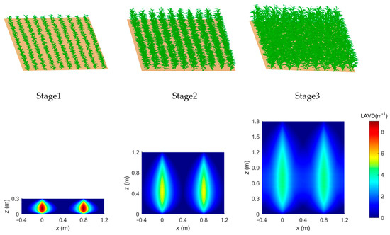
Figure 5. Scenes and LAVD of three growth stages.

Table 1. Row structure configuration of simulation scenes for the three growth stages.

Growth Stage	A (m)	H (m)	L (m)	LAI	θ01 (°)	β	ψ	e	Le (m)
Stage1	0.8	0.3	0.3	0.5	45	0.5	0.5	0.5	0.22
Stage2	0.8	1.2	0.4	1.6	45	0.5	0.5	0.5	0.30
Stage3	0.8	1.8	0.6	2.8	45	0.5	0.5	0.5	0.40

A is the distance between adjacent row centers. H is the canopy height. L is the half-width of the row structure. LAI is the leaf area index. L_e is the equivalent half-width of the row structure used for the Yan model.

We implement the BRDF model proposed by Yan et al. [2] for comparative analysis. This model incorporates the gap probability and hotspot effect, simulating radiance transfer within the canopy with good simulation accuracy. It utilizes the clumping index to correct deviations arising from leaf heterogeneity in the crop scene. Originally proposed in the V-NIR band [18] and later extended to the thermal infrared band [19,60], the clumping index serves as a critical parameter in leaf area index inversion [61,62,63,64]. Yan et al. [2] treated the row structure as homogeneous rectangular volumes and calculated the clumping index in the upper hemisphere space, while neglecting the heterogeneity within the row structure. Here, the structural parameters of the three stages used in the Yan model are slightly different from those of the new model. We use the equivalent half-width (L_e) for the rectangular row structure. L_e is the average length of leaves in the scene and is calculated in Table 1. Since the crop canopy is closed at stage 3, the Yan model treats it as a continuous canopy, with a calculated L_e value exceeding the half distance between adjacent row centers being capped at that maximum. A spherical LIDF is adopted for the Yan model. For all scenes, parameters unrelated to row structure, namely the solar azimuth and zenith angles, are assigned identical values in both the new model and the Yan model, as shown in Table 2.

Table 2. Input parameters of scenes other than row structure.

θs (°)	φs (°)
30	120

θ_s is the solar zenith angle. φ_s is the solar azimuth angle.

The spatial distributions of LAVD across three scenes are presented in Figure 5. A consistent spatial pattern emerges: maximum LAVD values occur at row centers, forming distinct drop-shaped distributions that decay radially toward inter-row spaces. It is evident that significant spatial heterogeneity persists throughout all growth stages, extending to stage3 (maturity stage) when canopy closure is achieved. Specifically, the wavelengths at 670 nm and 850 nm are selected to represent the red and NIR bands, respectively, which can effectively capture the distinct reflectance characteristics exhibited by the canopy.

Considering the directionality of BRDF, it is presented on a polar map where the coordinate system represents zenith and azimuth angles. The angular coordinate corresponds to the azimuth angle, starting from the north and increasing clockwise. The radial distance from the center corresponds to the zenith angle (0° at the center, 90° at the outer circle). This projection allows for an intuitive visualization of the spherical data on a two-dimensional plane, clearly showing directional data.

The polar map of the BRDF simulated by the DART model, new model, and Yan model for row crops across three growth stages at 670 nm is presented in Figure 6. The BRDF in the visible domain is dominated by single scattering from soil and foliage, with negligible contributions from multiple scattering. Compared to the Yan model, the new model shows stronger agreement with the DART model in the red band. At the first growth stage, the scene exhibits alternating vegetation rows and bare soil. When the viewing azimuth aligns parallel to the row azimuth, increased soil exposure generates a distinctive warm belt in BRDF polar maps. When viewing geometry aligns parallel to the row direction, increased soil exposure generates a distinctive warm belt in BRDF polar maps. Further analysis revealed that the R3T model underestimates the BRDF at the hotspot, and the exact reasons for this require further investigation. At the second growth stage, both simulation results of the DART model and R3T model show an obvious row effect. The Yan model displays a weak row effect, detectable only under large zenith angles along the row direction. Moreover, a lower belt appears on the side opposite to the solar direction in the BRDF polar maps of both the DART model and new model, whereas the Yan model fails to express this feature. Table 3 quantifies the BRDF agreement between the R3T model and DART model, demonstrating strong consistency with the RMSE (root mean square error) of 10⁻³ and rRMSE (relative root mean square error) below 7.50% in the red band.

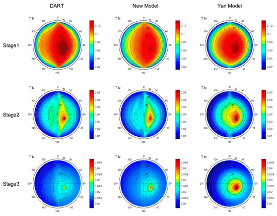
Figure 6. Polar plots of simulated BRDF in the red band (670 nm).

Table 3. Comparison of BRDF (R2 and RMSE) between the DART and R3T models.

Growth Stage	Statistics	BRDF_Red	BRDF_NIR	BRDF_NIR_1	BRDF_NIR_m
Stage1	R	0.87	0.93	0.94	0.88
	R2	0.9710	0.8769	0.8795	0.9637
	RMSE	0.0040	0.0098	0.0066	0.0052
	rRMSE	3.96%	2.92%	2.84%	5.56%
	MAD	−0.0069	−0.0076	−0.0036	−0.0039
Stage2	R	0.84	1.02	0.99	1.00
	R2	0.9448	0.9151	0.9109	0.9358
	RMSE	0.0023	0.0134	0.0079	0.0067
	rRMSE	7.50%	3.48%	4.26%	3.32%
	MAD	−0.0037	0.0032	0.0021	0.0012
Stage3	R	0.93	0.90	0.85	0.70
	R2	0.9121	0.8400	0.8585	0.7936
	RMSE	0.0011	0.0131	0.0093	0.0058
	rRMSE	6.10%	2.99%	3.45%	3.01%
	MAD	0.0003	0.0111	0.0123	0.0043

BRDF_red is the BRDF in the red band. BRDF_NIR is the BRDF in the NIR band. BRDF_NIR_1 is the single-scattering BRDF in the NIR band. BRDF_NIR_m is the multiple-scattering BRDF in the NIR band. R is the correlation coefficient. RMSE is the root mean square error. rRMSE is the relative root mean square error. R² is the coefficient of determination. MAD is the mean absolute deviation, positive for overestimation and negative for underestimation.

The polar map of the BRDF simulated by the DART model, R3T model, and Yan model for row crops across three growth stages at 850 nm is presented in Figure 7. Compared to the Yan model, the R3T model exhibits superior consistency with the DART model in the NIR band, with discrepancy not exceeding 3.48% (Table 3). The Yan model exhibits significant underestimation across all viewing directions and growth stages. To further analyze discrepancies among the three models, we partitioned the BRDF in the NIR band into two components: single-scattering BRDF (Figure 8) and multiple-scattering BRDF (Figure 9). Both the single and multiple scattering contribute a lot to the overall BRDF in the NIR band. At the first growth stage, both the R3T model and the Yan model underestimate the BRDF at the hotspot. For multiple scattering in the NIR band, the R3T model agrees with the DART model with an rRMSE below 5.56%, while the Yan model significantly underestimates the multiple-scattering BRDF. Further analysis reveals that multiple scattering for both stage2 and stage3 exhibits a distinct row effect: lower BRDF values occur when the viewing azimuth angle is aligned with the row azimuth, and multiple scattering significantly increases at large viewing zenith angles. However, multiple scattering at stage3 simulated by the Yan model exhibits exclusive zenith dependence with negligible azimuthal variation, consistent with homogeneous canopy scattering properties. This result indicates that despite mature canopy closure at the maturity stage, persistent spatial heterogeneity in row crops induces a row effect.

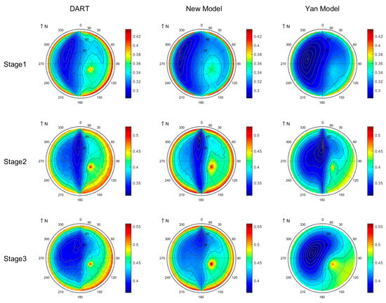
Figure 7. Polar plots of simulated BRDF in the NIR band (850 nm).

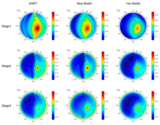
Figure 8. Polar plots of simulated single-scattering BRDF in the NIR band (850 nm).

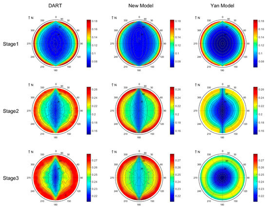
Figure 9. Polar plots of simulated multiple-scattering BRDF in the NIR band (850 nm).

4. Discussion

4.1. Sensitivity Analysis

Canopy structure critically influences the BRDF. A sensitivity analysis was conducted to investigate how LAVD and simulated BRDF respond to three control parameters. Stage2 (jointing stage) was selected for the sensitivity analysis. The jointing growth stage is the key growth stage for crops. At this stage, crops have completed most of the vegetative growth, having a great impact on the light transmission. Therefore, the variations in three control parameters can be well manifested in the canopy structure. In addition, crop size remains insufficient to cover bare soil between rows, facilitating the observation of row effect. More importantly, the sensitivity analysis of crops during the jointing stage holds significant importance for the parameter inversion, growth monitoring, and yield estimation of crops [65].

The value ranges and step values of the three control parameters are specified in Table 4. In each analysis, only one input parameter is varied incrementally according to its defined range and step value while other parameters remain constant (the same as those of stage2 in Table 1).

Table 4. Ranges and step values of the three control parameters for sensitivity analysis.

	Min Value	Max Value	Step Value
β	0	1	0.25
ψ	−1	1	0.50
e	0	1	0.25

(1)

Leaf Area Volume Density (LAVD)

The three control parameters directly govern the spatial distribution of LAVD, thereby propagating to the BRDF. The sensitivities of the three control parameters on LAVD are analyzed. Figure 10 shows how the horizontal and vertical distribution of LAVD varies with three control parameters. Parameter β modulates the horizontal distribution of LAVD without affecting its vertical distribution. With constant LAI and other parameters, increasing β reduces the leaf width far away from row centers. This causes LAVD to increase near row centers while decreasing far away from them. Parameter ψ modulates vertical LAVD distribution by governing leaf length, and this influence propagates to horizontal LAVD distribution. As ψ approaches 0, reduced leaf length variability diminishes LAVD vertical variability. As ψ = 0, LAVD becomes vertically uniform. Horizontally, as the absolute value of ψ approaches one, leaf clustering toward row centers enhances LAVD at row centers while reducing it farther away. Parameter e modulates the horizontal distribution of LAVD without affecting the vertical distribution. As e increases, leaves tend to orient perpendicular to the row direction. This causes LAVD to decrease at row centers while decreasing farther away. Concurrently, the position of maximum LAVD progressively shifts away from the row center.

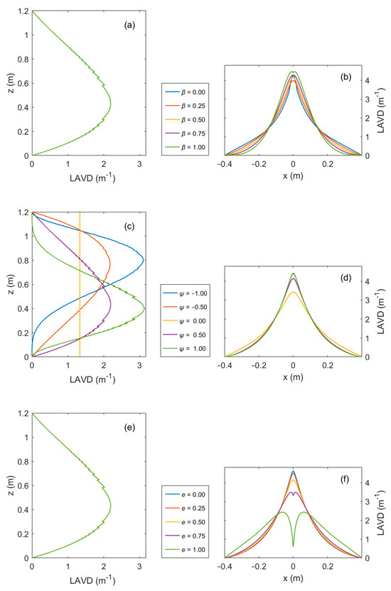
Figure 10. Single-factor sensitivity analysis of vertical and horizontal distribution of LAVD. (a), (c) and (e): The vertical distribution of LAVD varies with e, β, and ψ, respectively. (b), (d) and (f): The horizontal distribution of LAVD varies with e, β, and ψ, respectively. Other parameters are the same as in Table 1.

We adopt the coefficient of variation (CV) to quantify the heterogeneity of LAVD spatial distribution, shown in Figure 11. The CV, defined as the ratio of the standard deviation to the mean value, is a standardized measure of dispersion.

$${CV}_D={\displaystyle \frac{{\sigma }_D}{{\mu }_D}}\times 100\%$$

(16)

$${\mu }_D={\displaystyle \frac{{\int }_0^H{\int }_0^{A}D(x,z)\mathrm{d}x \mathrm{d}z}{A·H}}$$

(17)

$${\sigma }_D=\sqrt{{\displaystyle \frac{{\int }_0^H{\int }_0^A{\left(D\right(x,z)-{\mu }_D)}^2\mathrm{d}x \mathrm{d}z}{A·H}}}$$

(18)

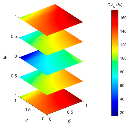
Figure 11. The spatial heterogeneity of LAVD varies with e, β, and ψ, respectively. CV, coefficient of variation.

A high CV value indicates a high degree of heterogeneity. Further analysis indicates that when the absolute value of φ increases to one, e approaches zero, and β approaches one, the heterogeneity of LAVD increases, and the CV reaches up to 170.95%. The peak heterogeneity appears when the leaf azimuth is uniformly distributed and the leaf shape and envelope of the row structure deviate from the rectangle. Notably, the minimum CV reaches 14.46%.

(2)

Bidirectional Reflectance Distribution Function (BRDF)

To highlight the effect of canopy structure on single scattering and multiple scattering, we conduct the sensitivity analysis in the NIR band at 850 nm. Two viewing planes are selected to investigate the effects of the three control parameters on BRDF: the solar principal plane (SPP, viewing azimuth angle aligned with solar azimuth angle) and the cross principal plane (CPP, viewing azimuth angle perpendicular to solar azimuth angle).

Parameter β varies from zero to one at an increment of 0.25. As illustrated in Figure 12a, the BRDF decreases with increasing β except for large zenith angles. Notably, the tendency is extremely pronounced at the darkspot. The BRDF of the darkspot decreases approximately linearly with increasing β (Figure 13a).

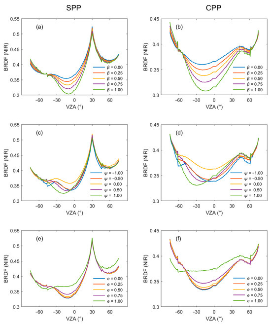
Figure 12. Single-factor sensitivity analysis of three control parameters in the NIR band (850 nm). SPP, the solar principal plane. CPP, the cross principal plane. VZA is the viewing zenith angle. (a) and (b): Sensitivity analysis of β in SPP and CPP, respectively. (c) and (d): Sensitivity analysis of ψ in SPP and CPP, respectively. (e) and (f): Sensitivity analysis of e in SPP and CPP, respectively. Other parameters are the same as in Table 1.

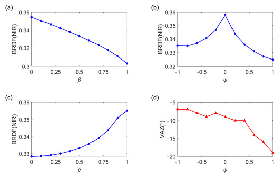
Figure 13. Sensitivity analysis of three control parameters on the BRDF and zenith angle of the darkspot in the NIR band (850 nm). (a–c) The BRDF of the darkspot varies with β, ψ, and e, respectively. (d) The zenith angle of the darkspot varies with ψ. Other parameters are the same as in Table 1.

Parameter ψ varies from −1 to 1 at an increment of 0.5. The influence of three control parameters on both the BRDF value and zenith angle of the darkspot is quantified in Figure 13b. To better present the effect of parameters on BRDF, reduced step values are adopted for the parameter variations in Figure 13. The impacts of ψ on BRDF are primarily manifested in both the BRDF value and the angular position of the darkspot. As shown in Figure 13b, the BRDF at the darkspot exhibits an initial ascent followed by a progressive decline with ψ varying from −1 to 1. The maximum BRDF for the darkspot appears at ψ = 0, corresponding to a rectangular row structure. Moreover, higher BRDF values are yielded by negative ψ compared to the positive ψ at equivalent absolute values. This indicates that higher BRDF values are observed when leaves are longer in the upper part of the canopy compared to the scene with longer leaves in the lower part. Furthermore, the variation in the zenith angle of the darkspot with ψ is shown in Figure 13d. As ψ increases, the zenith angle of the darkspot increases. When leaves in the upper canopy are longer, a low BRDF appears near the nadir.

Parameter e varies from zero to one at an increment of 0.25. Similar to β, parameter e significantly affects the BRDF of the darkspot without affecting its zenith angle. The BRDF value of the darkspot increases as e increases (Figure 13c), showing an approximately exponential relationship.

Figure 14 shows the variation in the BRDF value in the darkspot direction with three control parameters, with a range of 0.08 and a high relative range of 22.6%. Here, the range of is obtained by subtracting the minimum value from the maximum value.

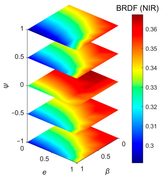
Figure 14. BRDF value of darkspot direction in NIR band. θ_s = 30°. φ_s = 120°.

(3)

Correlation Between the LAVD Spatial Heterogeneity and the BRDF

Figure 11 and Figure 14 reveal a strong negative correlation between the LAVD spatial heterogeneity and BRDF in the darkspot direction: as LAVD spatial heterogeneity increases, the BRDF value decreases. High LAVD heterogeneity induces a greater degree of leaf clumping, which increases soil exposure while reducing vegetation visibility. Given that soil reflectance is lower than leaf reflectance in the NIR band, this situation leads to an overall reduction in canopy reflectance. Conversely, a homogeneous LAVD distribution improves vegetation visibility while reducing soil exposure, thereby increasing the BRDF value. However, the Yan model significantly underestimates the BRDF across the three stages (Figure 7), which can be attributable to inaccurate parameterization of the G-function and Γ-function. This discrepancy highlights the critical influence of leaf inclination distribution on BRDF simulations and underscores the necessity of refined canopy structural characterization.

In contrast, the BRDF in the hotspot direction exhibits only minimal variation with the three control parameters (Figure 12). This phenomenon can be explained by the solar zenith angle being set at 30°, which allows sunlight to penetrate the canopy obliquely, thereby mitigating the influence of LAVD heterogeneity along the light path. As illustrated in Figure 15, this effect diminishes when the sun is at the nadir, under which condition both the darkspot and hotspot BRDF become more responsive to the control parameters compared to other solar zenith angles.

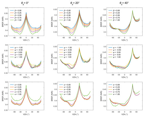
Figure 15. The BRDF in the SPP (solar principal plane) at different solar zenith angles. θ_s is the solar zenith angle. φ_s is the solar azimuth angle. φ_s = 120°.

4.2. Potential Applications

The new model adopts three control parameters to simulate the spatial distribution of LAVD, improving the simulation capability for row crops with a heterogeneous row structure. This model can be applied in parameter inversion involving row crops. Compared with the previous models, it provides more information, with high precision, about the row structure, such as the LAI, canopy height, row width, row spacing, and so on. Furthermore, it facilitates growth monitoring, drought prediction, and yield estimation for row crops.

4.3. The Determination of Three Control Parameters

To further facilitate the application of the new model, such as for parameter inversion and digital twin, three control parameters should be predetermined. Given that each species has a unique leaf shape, Mõttus et al. [36] identified β as a species-specific parameter and estimated its value through measurements. By extending this logic, it is reasonable to hypothesize that parameters e and ψ are likewise species-specific, as the leaf length and azimuth are also physiological characteristics for each species. Consequently, these parameters can be determined through measurements.

4.4. Model Limitations

While the proposed model represents a significant step forward, further refinements are possible to improve its depiction of a row crop canopy. One key area for enhancement lies in the representation of the canopy structure for row crops, especially the complex vertical heterogeneity inherent in the canopy. Beyond variability in leaf length, the canopy of row crops displays additional vertically stratified properties that are not yet fully captured. For example, observations show that leaf azimuth angular dispersion shows clear vertical stratification [66,67]. Basal leaves exhibit lateral clustering of azimuth angles with reduced dispersion, whereas apical leaves exhibit uniformly distributed azimuth orientations. This vertical stratification also extends to leaf zenith angles. Apical leaves in the maize canopy typically display an erectophile orientation, namely, straight leaves [68]. These stratified traits are central to the interception and scattering of light and energy exchange rate in canopies. Another important aspect for enhancement involves capturing the dynamic changes throughout the crop life cycle. Leaf biochemical constituent parameters, such as chlorophyll and water content, vary considerably with growth stages, directly influencing leaf optical properties and canopy reflectance. Additionally, to make the model suitable for the whole life cycle of row crops, the model should incorporate the effects of reproductive organs, such as ears for wheat and tassels for maize, which become significant structural and functional components during the maturity stage [34,69]. Therefore, future research regarding this model will integrate these vertically stratified traits and the effects of reproductive structures. These enhancements are expected to improve the model’s biophysical realism and its accuracy in simulating light interception and radiative transfer, ultimately leading to more robust applications in crop modeling.

5. Conclusions

In this paper, a new model for row crops is proposed. By introducing three control parameters, the new model accounts for horizontal and vertical heterogeneity within the canopy simultaneously. Validation results demonstrate that the model achieved high accuracy in BRDF simulation across three growth stages of row crops. Another key advantage of the new model is its ability to accurately represent canopy structure throughout the entire life cycle, effectively bridging the gap between discrete row-structure models and continuous vegetation models. Furthermore, this model reveals that even when the row crop canopy appears visually continuous, it retains substantial inter-row heterogeneity, which exerts a pronounced influence on the BRDF. Sensitivity analysis shows that the three control parameters significantly affect reflectance in the darkspot direction. Neglecting LAVD heterogeneity leads to a maximum error of approximately 22.6% in darkspot reflectance; such an error is not ignorable in quantitative remote sensing applications. Therefore, we recommend the use of this model for BRDF simulation and parameter inversion involving row crops.

References

- Zhao, F.; Gu, X.; Verhoef, W.; Wang, Q.; Yu, T.; Liu, Q.; Huang, H.; Qin, W.; Chen, L.; Zhao, H. A Spectral Directional Reflectance Model of Row Crops. Remote Sens. Environ. 2010, 114, 265–285. [Google Scholar] [CrossRef]
- Yan, B.; Xu, X.; Fan, W. A Unified Canopy Bidirectional Reflectance (BRDF) Model for Row Ceops. Sci. China Earth Sci. 2012, 55, 824–836. [Google Scholar] [CrossRef]
- Jackson, R.D.; Reginato, R.J.; Pinter, P.J.; Idso, S.B. Plant Canopy Information Extraction from Composite Scene Reflectance of Row Crops. Appl. Opt. 1979, 18, 3775. [Google Scholar] [CrossRef] [PubMed]
- Li, Y.; Gao, J.; Zha, Y. Impact of Rice Canopy Structure on Canopy Reflectance Spectra. In Proceedings of the Remote Sensing and Space Technology for Multidisciplinary Research and Applications, Beijing, China, 19–24 May 2005; Tong, Q., Chen, X., Huang, A., Gao, W., Eds.; SPIE: Cergy-Pontoise, France, 2006; p. 61990E. [Google Scholar]
- Zhou, G.; Tian, C.; Han, Y.; Niu, C.; Miao, H.; Jing, G.; Lopez, F.P.A.; Yan, G.; Najjar, H.S.M.; Zhao, F.; et al. Canopy Reflectance Modeling of Row Aquatic Vegetation: AVRM and AVMC. Remote Sens. Environ. 2024, 311, 114296. [Google Scholar] [CrossRef]
- Meggio, F.; Zarco-Tejada, P.J.; Miller, J.R.; Martín, P.; González, M.R.; Berjón, A. Row Orientation and Viewing Geometry Effects on Row-Structured Vine Crops for Chlorophyll Content Estimation. Can. J. Remote Sens. 2008, 34, 220–234. [Google Scholar] [CrossRef]
- Li, D.; Chen, J.M.; Zhang, X.; Yan, Y.; Zhu, J.; Zheng, H.; Zhou, K.; Yao, X.; Tian, Y.; Zhu, Y.; et al. Improved Estimation of Leaf Chlorophyll Content of Row Crops from Canopy Reflectance Spectra through Minimizing Canopy Structural Effects and Optimizing Off-Noon Observation Time. Remote Sens. Environ. 2020, 248, 111985. [Google Scholar] [CrossRef]
- Ma, X.; Lu, L.; Ding, J.; Zhang, F.; He, B. Estimating Fractional Vegetation Cover of Row Crops from High Spatial Resolution Image. Remote Sens. 2021, 13, 3874. [Google Scholar] [CrossRef]
- Zhang, B.; Fan, W.; Xu, X.; Liu, Y. FAPAR and BRDF Simulation for Row Crop Using Monte Carlo Method. In Proceedings of the 2014 IEEE Geoscience and Remote Sensing Symposium, Quebec City, QC, Canada, 13–18 July 2014; IEEE: New York, NY, USA, 2014; pp. 812–815. [Google Scholar]
- Jackson, J.E.; Palmer, J.W. Interception of Light by Model Hedgerow Orchards in Relation to Latitude, Time of Year and Hedgerow Configuration and Orientation. J. Appl. Ecol. 1972, 9, 341. [Google Scholar] [CrossRef]
- Kimes, D.S. Remote Sensing of Row Crop Structure and Component Temperatures Using Directional Radiometric Temperatures and Inversion Techniques. Remote Sens. Environ. 1983, 13, 33–55. [Google Scholar] [CrossRef]
- Chen, L.; Liu, Q.; Fan, W.; Li, X.; Xiao, Q.; Yan, G.; Tian, G. A Bi-Directional Gap Model for Simulating the Directional Thermal Radiance of Row Crops. Sci. China Ser. D Earth Sci. 2002, 45, 1087–1098. [Google Scholar] [CrossRef]
- Li, X.; Strahler, A.H. Modeling the Gap Probability of a Discontinuous Vegetation Canopy. IEEE Trans. Geosci. Remote Sens. 1988, 26, 161–170. [Google Scholar] [CrossRef]
- Kuusk, A. The Hot-Spot Effect of a Uniform Vegetative Cover. Sov. J. Remote Sens. 1985, 3, 645–658. [Google Scholar]
- Yan, G. Thermal Bidirectional Gap Probability Model for Row Crop Canopies and Validation. Sci. China Ser. D 2003, 46, 1241. [Google Scholar] [CrossRef]
- Jupp, D.L.B.; Strahler, A.H. A Hotspot Model for Leaf Canopies. Remote Sens. Environ. 1991, 38, 193–210. [Google Scholar] [CrossRef]
- Peng, J.; Fan, W.; Wang, L.; Xu, X.; Li, J.; Zhang, B.; Tian, D. Modeling the Directional Clumping Index of Crop and Forest. Remote Sens. 2018, 10, 1576. [Google Scholar] [CrossRef]
- Nilson, T. A Theoretical Analysis of the Frequency of Gaps in Plant Stands. Agric. Meteorol. 1971, 8, 25–38. [Google Scholar] [CrossRef]
- Yu, T.; Tian, G.; Legrand, M.; Baret, F.; Hanocq, J.-F.; Bosseno, R.; Zhang, Y. Modeling Directional Brightness Temperature over a Maize Canopy in Row Structure. IEEE Trans. Geosci. Remote Sens. 2004, 42, 2290–2304. [Google Scholar] [CrossRef]
- Li, X.; Strahler, A. Geometric-Optical Modeling of a Conifer Forest Canopy. IEEE Trans. Geosci. Remote Sens. 1985, GE-23, 705–721. [Google Scholar] [CrossRef]
- Verbrugghe, M.; Cierniewski, J. Effects of Sun and View Geometries on Cotton Bidirectional Reflectance. Test of a Geometrical Model. Remote Sens. Environ. 1995, 54, 189–197. [Google Scholar] [CrossRef]
- Ma, X.; Liu, Y. A Modified Geometrical Optical Model of Row Crops Considering Multiple Scattering Frame. Remote Sens. 2020, 12, 3600. [Google Scholar] [CrossRef]
- Norman, J.M.; Welles, J.M. Radiative Transfer in an Array of Canopies. Agron. J. 1983, 75, 481–488. [Google Scholar] [CrossRef]
- Chen, J.M.; Leblanc, S.G. Multiple-Scattering Scheme Useful for Geometric Optical Modeling. IEEE Trans. Geosci. Remote Sens. 2001, 39, 1061–1071. [Google Scholar] [CrossRef]
- Li, X.; Woodcock, C.E. A Hybrid Geometric Optical-Radiative Transfer Approach for Modeling Albedo and Directional Reflectance of Discontinuous Canopies. IEEE Trans. Geosci. Remote Sens. 1995, 33, 466–480. [Google Scholar] [CrossRef]
- Verhoef, W. Earth Observation Modeling Based on Layer Scattering Matrices. Remote Sens. Environ. 1985, 17, 165–178. [Google Scholar] [CrossRef]
- Liou, K.N. An Introduction to Atmospheric Radiation; Academic Press: Cambridge, MA, USA, 2002. [Google Scholar]
- Suits, G.H. Extension of a Uniform Canopy Reflectance Model to Include Row Effects. Remote Sens. Environ. 1983, 13, 113–129. [Google Scholar] [CrossRef]
- Suits, G. The Calculation of the Directional Reflectance of a Vegetative Canopy. Remote Sens. Environ. 1971, 2, 117–125. [Google Scholar] [CrossRef]
- Zhou, K.; Guo, Y.; Geng, Y.; Zhu, Y.; Cao, W.; Tian, Y. Development of a Novel Bidirectional Canopy Reflectance Model for Row-Planted Rice and Wheat. Remote Sens. 2014, 6, 7632–7659. [Google Scholar] [CrossRef]
- Verhoef, W.; Jia, L.; Xiao, Q.; Su, Z. Unified Optical-Thermal Four-Stream Radiative Transfer Theory for Homogeneous Vegetation Canopies. IEEE Trans. Geosci. Remote Sens. 2007, 45, 1808–1822. [Google Scholar] [CrossRef]
- Wang, Q.; Li, P. Canopy Vertical Heterogeneity Plays a Critical Role in Reflectance Simulation. Agric. For. Meteorol. 2013, 169, 111–121. [Google Scholar] [CrossRef]
- Zhao, C.; Li, H.; Li, P.; Yang, G.; Gu, X.; Lan, Y. Effect of Vertical Distribution of Crop Structure and Biochemical Parameters of Winter Wheat on Canopy Reflectance Characteristics and Spectral Indices. IEEE Trans. Geosci. Remote Sens. 2017, 55, 236–247. [Google Scholar] [CrossRef]
- Du, Y.; Liu, Q.; Chen, L.; Liu, Q.; Yu, T. Modeling Directional Brightness Temperature of the Winter Wheat Canopy at the Ear Stage. IEEE Trans. Geosci. Remote Sens. 2007, 45, 3721–3739. [Google Scholar] [CrossRef]
- Du, Y.; Cao, B.; Li, H.; Bian, Z.; Qin, B.; Xiao, Q.; Liu, Q.; Zeng, Y.; Su, Z. Modeling Directional Brightness Temperature (DBT) over Crop Canopy with Effects of Intra-Row Heterogeneity. Remote Sens. 2020, 12, 2667. [Google Scholar] [CrossRef]
- Mõttus, M.; Ross, V.; Ross, J. Shape and Area of Simple Narrow Leaves. Proc. Est. Acad. Sci. Biology. Ecol. 2002, 51, 147. [Google Scholar] [CrossRef]
- Mottus, M. Measurement and Modelling of the Vertical Distribution of Sunflecks, Penumbra and Umbra in Willow Coppice. Agric. For. Meteorol. 2004, 121, 79–91. [Google Scholar] [CrossRef]
- Mõttus, M.; Sulev, M.; Lang, M. Estimation of Crown Volume for a Geometric Radiation Model from Detailed Measurements of Tree Structure. Ecol. Model. 2006, 198, 506–514. [Google Scholar] [CrossRef]
- Mõttus, M. Photon Recollision Probability in Discrete Crown Canopies. Remote Sens. Environ. 2007, 110, 176–185. [Google Scholar] [CrossRef]
- Mõttus, M.; Stenberg, P.; Rautiainen, M. Photon Recollision Probability in Heterogeneous Forest Canopies: Compatibility with a Hybrid GO Model. J. Geophys. Res. 2007, 112, D03104. [Google Scholar] [CrossRef]
- Mõttus, M.; Pham, P.; Halme, E.; Molinier, M.; Cu, H.; Laaksonen, J. TAIGA: A Novel Dataset for Multitask Learning of Continuous and Categorical Forest Variables From Hyperspectral Imagery. IEEE Trans. Geosci. Remote Sens. 2022, 60, 5521711. [Google Scholar] [CrossRef]
- Liu, W.; Mõttus, M.; Gastellu-Etchegorry, J.-P.; Fang, H.; Atherton, J. Seasonal and Vertical Variation in Canopy Structure and Leaf Spectral Properties Determine the Canopy Reflectance of a Rice Field. Agric. For. Meteorol. 2024, 355, 110132. [Google Scholar] [CrossRef]
- Verhoef, W. Light Scattering by Leaf Layers with Application to Canopy Reflectance Modeling: The SAIL Model. Remote Sens. Environ. 1984, 16, 125–141. [Google Scholar] [CrossRef]
- Wu, M.; Zhu, Q.; Wang, J.; Xiang, Y.; Shuai, Y.; Tang, S. The BRDF Model and Analysis of Hotspot Effect of Row Crops. In Proceedings of the IEEE International Geoscience and Remote Sensing Symposium, Toronto, ON, Canada, 24–28 June 2002; IEEE: New York, NY, USA, 2002; Volume 6, pp. 3302–3304. [Google Scholar]
- Ma, X.; Wang, T.; Lu, L. A Refined Four-Stream Radiative Transfer Model for Row-Planted Crops. Remote Sens. 2020, 12, 1290. [Google Scholar] [CrossRef]
- Maddonni, G.; Chelle, M.; Drouet, J.; Andrieu, B. Light Interception of Contrasting Azimuth Canopies under Square and Rectangular Plant Spatial Distributions: Simulations and Crop Measurements. Field Crops Res. 2001, 70, 1–13. [Google Scholar] [CrossRef]
- Teh, C.B.S.; Simmonds, L.P.; Wheeler, T.R. An Equation for Irregular Distributions of Leaf Azimuth Density. Agric. For. Meteorol. 2000, 102, 223–234. [Google Scholar] [CrossRef]
- Torres, G.M.; Koller, A.; Taylor, R.; Raun, W.R. SEED-ORIENTED PLANTING IMPROVES LIGHT INTERCEPTION, RADIATION USE EFFICIENCY AND GRAIN YIELD OF MAIZE (Zea mays L.). Ex. Agric. 2017, 53, 210–225. [Google Scholar] [CrossRef]
- Fortin, M.-C.; Pierce, F.J. Leaf Azimuth in Strip-Intercropped Corn. Agron. J. 1996, 88, 6–9. [Google Scholar] [CrossRef]
- Serouart, M.; Lopez-Lozano, R.; Daubige, G.; Baumont, M.; Escale, B.; De Solan, B.; Baret, F. Analyzing Changes in Maize Leaves Orientation Due to GxExM Using an Automatic Method from RGB Images. Plant Phenomics 2023, 5, 0046. [Google Scholar] [CrossRef]
- Yang, P.; Verhoef, W.; Van Der Tol, C. The mSCOPE Model: A Simple Adaptation to the SCOPE Model to Describe Reflectance, Fluorescence and Photosynthesis of Vertically Heterogeneous Canopies. Remote Sens. Environ. 2017, 201, 1–11. [Google Scholar] [CrossRef]
- Watanabe, T.; Hanan, J.S.; Room, P.M.; Hasegawa, T.; Nakagawa, H.; Takahashi, W. Rice Morphogenesis and Plant Architecture: Measurement, Specification and the Reconstruction of Structural Development by 3D Architectural Modelling. Ann. Bot. 2005, 95, 1131–1143. [Google Scholar] [CrossRef] [PubMed]
- Stenberg, P. A Note on the G-Function for Needle Leaf Canopies. Agric. For. Meteorol. 2006, 136, 76–79. [Google Scholar] [CrossRef]
- Ross, J. The Radiation Regime and Architecture of Plant Stands; Tasks for Vegetation Ences; Springer: Dordrecht, The Netherlands, 1981. [Google Scholar]
- Weiss, M.; Baret, F.; Smith, G.J.; Jonckheere, I.; Coppin, P. Review of Methods for in Situ Leaf Area Index (LAI) Determination. Agric. For. Meteorol. 2004, 121, 37–53. [Google Scholar] [CrossRef]
- Nilson, T.; Kuusk, A. A Reflectance Model for the Homogeneous Plant Canopy and Its Inversion. Remote Sens. Environ. 1989, 27, 157–167. [Google Scholar] [CrossRef]
- Jacquemoud, S.; Baret, F. PROSPECT: A Model of Leaf Optical Properties Spectra. Remote Sens. Environ. 1990, 34, 75–91. [Google Scholar] [CrossRef]
- Féret, J.-B.; Berger, K.; De Boissieu, F.; Malenovský, Z. PROSPECT-PRO for Estimating Content of Nitrogen-Containing Leaf Proteins and Other Carbon-Based Constituents. Remote Sens. Environ. 2021, 252, 112173. [Google Scholar] [CrossRef]
- Gastellu-Etchegorry, J. Modeling Radiative Transfer in Heterogeneous 3-D Vegetation Canopies. Remote Sens. Environ. 1996, 58, 131–156. [Google Scholar] [CrossRef]
- Bian, Z.; Cao, B.; Li, H.; Du, Y.; Lagouarde, J.-P.; Xiao, Q.; Liu, Q. An Analytical Four-Component Directional Brightness Temperature Model for Crop and Forest Canopies. Remote Sens. Environ. 2018, 209, 731–746. [Google Scholar] [CrossRef]
- Bo, X.; Xie, D.; Wu, M.; Yan, G.; Mu, X. Leaf area index inversion corrected with clumping index of maize canopy. J. Beijing Norm. Univ. Nat. Sci. 2025, 61, 217–227. [Google Scholar]
- Ma, X.; Wang, T.; Lu, L.; Huang, H.; Ding, J.; Zhang, F. Developing a 3D Clumping Index Model to Improve Optical Measurement Accuracy of Crop Leaf Area Index. Field Crops Res. 2022, 275, 108361. [Google Scholar] [CrossRef]
- Hill, M.J.; Román, M.O.; Schaaf, C.B.; Hutley, L.; Brannstrom, C.; Etter, A.; Hanan, N.P. Characterizing Vegetation Cover in Global Savannas with an Annual Foliage Clumping Index Derived from the MODIS BRDF Product. Remote Sens. Environ. 2011, 115, 2008–2024. [Google Scholar] [CrossRef]
- Bao, Y. Estimation of Clumping Index and LAI from Terrestrial LiDAR Data. In Proceedings of the 2016 IEEE International Geoscience and Remote Sensing Symposium (IGARSS), Beijing, China, 10–15 July 2016; pp. 747–750. [Google Scholar]
- Yao, Y.; Liu, Q.; Liu, Q. Canopy Modeling and Validation for Row Planted Crops of Key Growth Stages. In Proceedings of the 2009 IEEE International Geoscience and Remote Sensing Symposium, Cape Town, South Africa, 12–17 July 2009; IEEE: New York, NY, USA, 2009; pp. II-686–II-689. [Google Scholar]
- Drouet, J.-L.; Moulia, B. Spatial Re-Orientation of Maize Leaves Affected by Initial Plant Orientation and Density. Agric. For. Meteorol. 1997, 88, 85–100. [Google Scholar] [CrossRef]
- Girardin, P.; Tollenaar, M. Effects of Intraspecific Interference on Maize Leaf Azimuth. Crop Sci. 1994, 34, 151–155. [Google Scholar] [CrossRef]
- Homem Antunes, M.A.; Walter-Shea, E.A.; Mesarch, M.A. Test of an Extended Mathematical Approach to Calculate Maize Leaf Area Index and Leaf Angle Distribution. Agric. For. Meteorol. 2001, 108, 45–53. [Google Scholar] [CrossRef]
- Li, W.; Jiang, J.; Weiss, M.; Madec, S.; Tison, F.; Philippe, B.; Comar, A.; Baret, F. Impact of the Reproductive Organs on Crop BRDF as Observed from a UAV. Remote Sens. Environ. 2021, 259, 112433. [Google Scholar] [CrossRef]
Disclaimer/Publisher’s Note: The statements, opinions and data contained in all publications are solely those of the individual author(s) and contributor(s) and not of MDPI and/or the editor(s). MDPI and/or the editor(s) disclaim responsibility for any injury to people or property resulting from any ideas, methods, instructions or products referred to in the content. |
© 2025 by the authors. Licensee MDPI, Basel, Switzerland. This article is an open access article distributed under the terms and conditions of the Creative Commons Attribution (CC BY) license (https://creativecommons.org/licenses/by/4.0/).