Design of Extensible Structured Interferometric Array Utilizing the “Coarray” Concept

Abstract

The optimum placement of receiving telescope antennas is a central topic for designing radio interferometric arrays, and this determines the performance of the obtained information. A variety of arrays are designed for different purposes, and they perform poorly in scalability. In this paper, we consider a subclass of structured sparse arrays, namely nested arrays, and examine the important role of “coarray” in interferometric synthesis imaging, which is utilized to design nested array configurations for a complete uniform Fourier plane coverage in both supersynthesis and instantaneous modes. Both nested arrays and the theory of the coarray have rich research achievements, and we apply them to astronomy to design arrays with good scalability and imaging performance. Simulated celestial source image retrieval performance validates the effectiveness of nested interferometric arrays.

1. Introduction

Interferometry, a promising technology, is applied to the fields of cosmology, astrophysics, astronomy, ionospheric physics, radar, and human–machine interaction [1,2,3,4,5,6]. An interferometric array detects spatial frequencies of the sky brightness function, the visibilities, in the Fourier plane (or uv-plane) by cross-correlating antenna pairs [7], and the set of measured spatial frequencies is a key aspect in the design of the interferometer [8]. For N antennas, there are $N(N-1)/2$ instantaneous measurements in the Fourier plane, which is insufficient for small numbers of antennas. As many radio sources of interest do not vary significantly over short time scales, the Fourier plane coverage can be improved by tracking the measurements with the Earth’s rotation, which is referred to as the supersynthesis process in radio astronomy [9]. However, for fast imaging, the instantaneous coverage is more important than the full coverage. As such, a central topic of telescope array design is how to arrange the antennas in an optimum configuration so that the sampling of the Fourier plane permits reconstruction of high-fidelity images. Most of the work on this topic mainly investigates the problem of telescope antenna placement under the principle of a complete Fourier plane sampling [10] or the lowest peak sidelobe level (PSL) in the angular domain [11]. In the absence of any prior information about the celestial object to be observed, a uniform uv distribution offers the desired sampling of the Fourier plane and a high signal-to-noise ratio with improved resolution.

When financial considerations permit, additional telescopes can be used to augment existing arrays, leading to increased astronomical information. Placing additional telescopes should not, however, require modification of the entire array and changing the locations and spacing between the different telescope units. In this case, array extensibility, where increased aperture and improved array response are achieved with each additional telescope and without altering existing array configurations, becomes important. In this respect, in addition to uniform coverage in the uv domain, designing interferometric arrays should permit future extensibility. This design condition is not well-addressed in the literature. Various algorithms, such as pseudodynamic programming [12], Particle Swarm Algorithm (PSO) [13], and hybrid Almost Difference Sets (ADSs) techniques [14], are applied to optimize element positions on each arm of a Y-shaped array in order to reduce redundancy in the Fourier plane sampling and suppress the PSL in the dirty beam. However, these employed heuristic approaches are computationally expensive, especially for arrays with large numbers of elements. Moreover, the underlying design procedure of these arrays does not lend itself to an extended or expanded array if need be. In essence, the design process must be repeated in its entirety, even if a single telescope is to be added to an existing configuration. As such, it does not yield scalable arrays and results in a totally different array structure with each new telescope.

Various kinds of structured sparse arrays have been investigated for high-resolution spatial spectrum sensing, such as minimum redundancy array (MRA) [15,16], minimum hole array (MHA) [17], and coprime array [18]. It is noted that both MRA and MHA only exist for a limited number of antennas, and none of these structured arrays are amenable for future extension. That is, when we increase the number of antennas, the entire array must change its original structure to maintain the minimum redundancy, the minimum hole, or the coprime properties.

Nested arrays [19], obtained by nesting two or more uniform linear arrays systematically, could generate a set of uniformly distributed virtual difference coarrays. Based on the nested structure, many works about optimizing array signal processing algorithms have been carried out, such as enhancing degrees of freedom (DOF) and achieving more sources’ direction of arrival (DOA) estimation [20,21].

This paper recognizes the important role of coarray [22] in interferometric imaging. Moreover, the nested configuration of radio telescopes is identified as an attractive design for array extensibility in both supersynthesis and instantaneous modes. As the nested array structure places more elements near the center of the array [23], this automatically leads to a higher sensor density in the center and a lower density moving outwards. This property mitigates the problem of insufficient Fourier components of lower spatial frequency due to the nature of Earth’s rotation in the supersynthesis mode. We apply nested configurations and the concept of coarray together to design arrays with good scalability and imaging performance.

The remaining part of this paper is organized as follows. The latent role of the coarray in aperture synthesis imaging is explained in Section 2. In Section 3, we present the design of extensible nested arrays. Supporting simulation results are provided in Section 4, while Section 5 contains the conclusion.

2. Coarray in Interferometric Synthesis Imaging

Assuming that the positions of array elements form the set, $S=\{{\mathbf{r}}_i,i=1,\dots ,N\}$, the corresponding difference coarray has positions $S_d=\{{\mathbf{r}}_i-{\mathbf{r}}_j,i,j=1,\dots ,N\}$. That is, the difference coarray is the set of pairwise differences of the array element positions. In radio astronomy, each pairwise difference $\mathbf{r}={\mathbf{r}}_i-{\mathbf{r}}_j$ is known as an interferometric “baseline”, and it plays a critical role in synthesis imaging. Short baselines correspond to lower spatial frequencies, which represent large-scale structures of the source image, while long baselines detect higher spatial frequencies, from which we can obtain subtle structures of the source image. Note that the longest baseline determines the resolution of retrieved images. Hence, by suitable construction of the original set S, the number of baselines can be substantially increased for a given number of physical antennas N, and a better uv-coverage can be obtained.

Define the image coordinate system $(p,q)$ to be fixed on the celestial sphere and centered in the imaging field of view (FOV). The source declination is denoted as $\delta$ and the observation time duration as H ($H\in [0,12]$, unit: hours). The visibility of the source, $V(u,v)$, is defined in a plane perpendicular to the source direction, with $(u,v)$ aligned to $(p,q)$. The visibility matrix $\mathbf{V}=\left[V\right(u,v\left)\right]$ is actually the correlation matrix in the uv-domain. Denoting the elevation of the baseline as $\epsilon$, the latitude as $\phi$, and the azimuth as $\psi$, the transformation between the spatial sampling point $(u,v)$ and the baseline vector $\mathbf{r}$ can be expressed as [9]:

$$\left[\begin{array}{c}u\\ v\end{array}\right]=\left[\begin{array}{ccc}sinh& cosh& 0\\ -sin\delta cosh& sin\delta sinh& cos\delta \end{array}\right]\left[\begin{array}{c}\Delta X\\ \Delta Y\\ \Delta Z\end{array}\right],$$

(1)

with

$$\left[\begin{array}{c}\Delta X\\ \Delta Y\\ \Delta Z\end{array}\right]=\left|\mathbf{r}\right|\left[\begin{array}{c}cos\phi sin\epsilon -sin\phi cos\epsilon cos\psi \\ cos\epsilon sin\psi \\ sin\phi sin\epsilon +cos\phi cos\epsilon cos\psi \end{array}\right],$$

(2)

where $\left|\mathbf{r}\right|$ denotes the baseline length, instant hour angle $h\in (-\frac{H\pi }{12},\frac{H\pi }{12})$ (unit: radians), and $\Delta X,\Delta Y,\Delta Z$ are measured in the unit of wavelength $\lambda$, i.e., a unit distance corresponds to one wavelength. Each baseline generates a point on the uv-plane in the instantaneous mode, whereas in a supersynthesis mode, each baseline vector tracks an arc of an ellipse in the uv-plane due to the Earth’s rotation. Assuming the time interval between taking two samplings to be $\Delta H$, each baseline corresponds to $(H/\Delta H)$ uv-points in the supersynthesis mode, compared to the one-to-one mapping in a snapshot observation. Note that the uv-coverage coincides with the difference coarray $S_d$ in the instantaneous mode at zenith, i.e., $\phi =\delta$, resulting in $u=\left|\mathbf{r}\right|sin\psi$ and $v=\left|\mathbf{r}\right|cos\psi$, and the visibility matrix $\mathbf{V}=\left[V\right(u,v\left)\right]$ equals the array correlation matrix in this case.

The well-known van Cittert–Zernike theorem [9] states that a 2D Fourier transform relationship exists between the visibilities $\mathbf{V}$ and the sky brightness $\mathbf{I}$, which is given by

$$\begin{array}{c}\hfill I(p,q)={\int }_{-\infty }^{\infty }{\int }_{-\infty }^{\infty }V(u,v)e^{j2\pi (up+vq)}dudv,\end{array}$$

(3)

which can be simply represented as

$$\begin{array}{c}\hfill I(p,q)\rightleftharpoons V(u,v),\end{array}$$

(4)

where ⇌ denotes the Fourier transformation pair.

Therefore, the discrete form of the imaging equation can be expressed as

$$\begin{array}{ccc}\hfill I(p,q)& =& \sum _{i=1}^{N_u}\sum _{j=1}^{N_v}V(u_i,v_j)e^{j2\pi (u_{i}p+v_{j}q)},\hfill \\ & =& {\mathbf{e}}^T\left(p\right)\mathbf{V}\tilde{\mathbf{e}}\left(q\right),\hfill \\ & =& {(\tilde{\mathbf{e}}\left(q\right)\otimes \mathbf{e}\left(p\right))}^T\mathbf{z},\hfill \end{array}$$

(5)

where $N_u$ and $N_v$ denote the numbers of sampling points in the u- and v-dimensions, respectively, $\mathbf{e}\left(p\right)={[e^{j2\pi u_{1}p},\dots ,e^{j2\pi u_{L}p}]}^T$, $\tilde{\mathbf{e}}\left(q\right)={[e^{j2\pi v_{1}q},\dots ,e^{j2\pi v_{M}q}]}^T$, ‘⊗’ denotes the Kronecker product, and $\mathbf{z}=\mathrm{vec}\left\{\mathbf{V}\right\}$ are the vectorized visibilities or equivalently the vectorized coarray measurements in the uv-plane.

The relationship between the measured visibility $V_{mea}(u,v)$ and the uv-coverage $C(u,v)$ can be denoted as

$$\begin{array}{c}\hfill V_{mea}(u,v)=C(u,v)c(u,v)V(u,v),\end{array}$$

(6)

where $c(u,v)$ is a weighting function for a better synthesized dirty beam.

Therefore, the measured source image $I_{mea}(p,q)$ can be obtained by inverse FFT of the measured visibility $V_{mea}(u,v)$

$$\begin{array}{c}\hfill I_{mea}(p,q)\rightleftharpoons V_{mea}(u,v).\end{array}$$

(7)

Thus, we can see that astronomical synthesis imaging is equivalent to beamforming with the uv-domain measurements [24] and the uv-coverage plays a vital role in image recovery performance.

3. Extensible Interferometric Array Design

We design nested interferometric arrays utilizing the mapping (one-to-one or one-to-$H/\Delta H$) between the coarray and uv-coverage. More specifically, we consider linear and “Y”-shaped nested configurations in the supersynthesis mode, cross-product and 2D nested configurations in the instantaneous mode.

3.1. Linear Nested Array

Different from the well-known Bracewell array [25], a two-level nested array is a concatenation of two uniform linear arrays (ULAs), where one ULA has $N_1$ elements with spacing $d_1$ and the other ULA has $N_2$ elements with spacing $d_2=(N_1+1)d_1$, i.e., $S=\{n{d}_1,n=0,\cdots ,N_1-1\}\cup \{d_1[n(N_1+1)-1],n=1,\cdots ,N_2\}$. The corresponding difference coarray is a filled ULA with $2N_2(N_1+1)-1$ elements, whose positions are given by $S_d=\{n{d}_1,n=-K,\dots ,K,K=N_2(N_1+1)-1\}$. A 14-element linear nested array with $N_1=N_2=7$ and its corresponding difference coarray are shown in Figure 1a,b, respectively. The position of the last element of the array is set as 8 km.

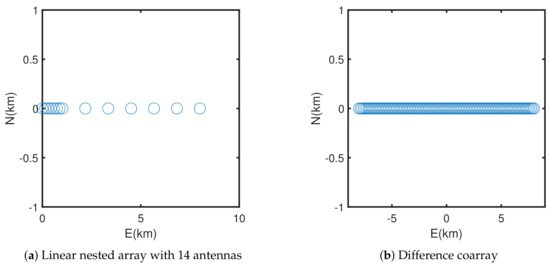
Figure 1. Configuration of linear nested array and corresponding difference coarray.

3.2. Y-Shaped Nested Array

Similar to the very large array (VLA) [26], we set the latitude and elevation of the Y-shaped nested array as $\phi =+{34}^{\circ },\epsilon =0^{\circ }$, and rotate the entire array by $5^{\circ }$ from the north–south direction to achieve a better uv-coverage at low declinations. Each arm of the “Y” extends up to 21 km and the innermost element on each arm is 0.84 km away from the center of the array. We design each arm of the Y-shaped array as a two-level linear nested array with $N_1=4$ and $N_2=5$ antennas as shown in Figure 2a. The corresponding difference coarray of the Y-shaped nested array is depicted in Figure 2b.

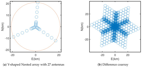
Figure 2. Configuration of Y-shaped nested array and corresponding difference coarray.

3.3. Cross-Product Nested Array

Compared to one-dimensional arrays, 2D arrays allow us to acquire more information from the source. An obvious way to construct a 2D extensible array is the cross-product of two linear nested arrays, i.e., $[b_n,d_m],thereinto,n=1,\cdots ,N,m=1,\cdots ,M$, where both $\{b_1,\cdots ,b_N\}$ and $\{d_1,\cdots ,d_M\}$ are linear nested sequences. An example is shown in Figure 3a, where two identical linear nested arrays with $N_1=12,N_2=5$ are utilized. The difference coarray of this cross-product nested array is a uniform rectangular array with aperture $b_N\times d_M$. Note that this method requires a total of $MN$ antennas and exhibits a high redundancy ratio. As such, a less-redundant 2D nested array design is more promising.

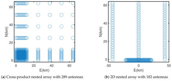
Figure 3. Configurations of cross-product and 2D nested arrays.

3.4. 2D Nested Array

We design a 2D nested array, which is the union of a dense array, containing sensors on a lattice described by the generator matrix ${\mathbf{N}}^d$, and a sparse array with sensors on a lattice generated by the generator matrix ${\mathbf{N}}^s={\mathbf{N}}^d\mathbf{P}$. Here, $\mathbf{P}=\mathrm{diag}(P_1,P_2)$ is a diagonal matrix with $P_1$ being a positive odd integer and $P_2$ being a positive integer. We adopt the offset configuration proposed in [27] in order to obtain more distinct baselines. Given $(2N_1^s+1)N_2^s+P_1{P}_2$ physical antennas, we place a total of $(2N_1^s+1)N_2^s$ sensors in the sparse array at locations

$${\mathbf{N}}^s{[m,n]}^T,\left|m\right|\le N_1^s,0\le n\le N_2^s-1,$$

(8)

where ${[m,n]}^T$ is a column vector of integer entries. The $P_1{P}_2$ dense array sensors are positioned at

$${\mathbf{N}}^d({[m,n]}^T-{[0,0.5]}^T),\left|m\right|\le \frac{P_1-1}{2},-P_2+1\le n\le 0.$$

(9)

The resulting difference coarray contains a rectangular uniformly filled subarray with virtual antenna positions

$$\begin{array}{ccc}\hfill {\mathbf{N}}^d({[m,n]}^T-{[0,0.5]}^T),& & \left|m\right|\le P_1{N}_1^s+\frac{P_1-1}{2},\hfill \\ & & -P_2{N}_2^s+1\le n\le P_2{N}_2^s.\hfill \end{array}$$

(10)

A 182-element 2D nested array is shown in Figure 3b.

4. Simulation Results

4.1. Example 1: Linear Nested Array

Consider the 14-element linear nested array of Figure 1a. The latitude and elevation of the array are selected as $\phi =+{34}^{\circ }$ and $\epsilon =0^{\circ }$, respectively. With the uv-coverage sampled with $N_u=N_v=128$ grids, Figure 4a depicts the uv-mask $\mathbf{M}\in {\{0,1\}}^{N_u\times N_v}$, corresponding to uv-coverage for a north-pole source (i.e., $\delta ={90}^{\circ }$) over a 12 h tracking with 5 min sampling interval. The corresponding entry of $\mathbf{M}$ for a grid is zero if no uv-points fall into that grid; otherwise, it assumes a unit value. The operating frequency is set to 3.6 GHz. Dirty beam, which is determined by the configuration of the array and affected by environmental factors, plays an important role in imaging recovery of interferometric telescopes [28]. In order to suppress sidelobes of the synthesized dirty beam, a rotationally symmetric 2D Gaussian weighting with a standard deviation of 20 is used. The dirty beam is shown in Figure 4b, which is obtained by a $512\times 512$ inverse FFT of the weighted uv-mask, where a zero-padding with a factor of four is applied to better illustrate the beampattern. The maximum uv aperture, measured in the unit of wavelength $\lambda$, is $1.92\times {10}^5$ and sampled with $N_u=N_v=128$ grids; each unit grid size is ${\Delta }_u={\Delta }_v=1.5\times {10}^3$. Thus, the maximum FOV is $2/\Delta u=275.0$ arc seconds. However, Figure 4b only plots an angular range within $\pm 34$ arc seconds to clearly illustrate the peak sidelobes. The angular resolution of the dirty beam is 0.66 arc seconds, and the PSL is $-17.85$ dB.

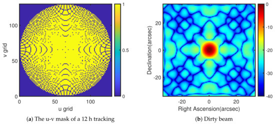
Figure 4. The u-v mask of linear nested array and corresponding dirty beam.

4.2. Example 2: Y-Shaped Nested Array

Considering the Y-shaped nested array plotted in Figure 2a, we repeat all the simulations in Section 4.1 with the exceptions that the tracking time is shortened to 8 h and the source declination is set as $\delta =+{34}^{\circ }$ (i.e., zenith observation). The uv-mask of the Y-shaped nested array is shown in Figure 5a. We can observe that the inner portion of the uv-mask is dense, while the outer portion is sparse. Hence, we can obtain more low spatial frequencies, which correspond to large-scale structures of celestial source. For the Y-shaped nested array in Figure 2a, the maximum uv aperture is $8.7\times {10}^5$. Sampling the uv-coverage with $N_u=N_v=128$ grids, each unit grid size is ${\Delta }_u={\Delta }_v=6.8\times {10}^3$. Therefore, the maximum FOV is $2/\Delta u=60.6$ arc seconds. The dirty beam of the Y-shaped nested array is depicted in Figure 5b. Similarly, Figure 5b plots an angular range within $\pm 7$ arc seconds for illustrating the peak sidelobes better. The angular resolution of the dirty beam is 0.14 arc seconds and the PSL is $-19.08$ dB.

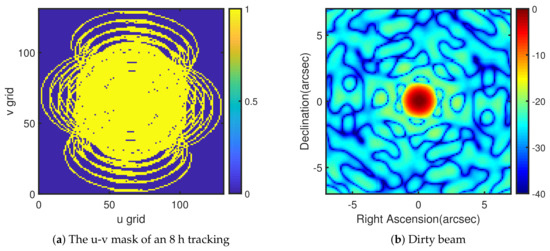
Figure 5. The u-v mask of Y-shaped nested array and corresponding dirty beam.

4.3. Example 3: Cross-Product and 2D Nested Arrays

The cross-product array of Figure 3a provides a complete uniform $128\times 128$ instantaneous uv-mask at zenith, which is shown in Figure 6a. Next, in order to reduce redundancy of the cross-product array, we consider the 2D nested array, shown in Figure 3b, with ${\mathbf{N}}^d=\left[\begin{array}{cc}1& 0\\ 0& 1\end{array}\right]$, $\mathbf{P}=\left[\begin{array}{cc}43& 0\\ 0& 2\end{array}\right],$ $N_1^s=1$ and $N_2^s=32$. The 2D nested array provides the same uv-coverage as the cross-product nested array but requires a total of only 182 antennas compared to 289 for the cross-product array, which shows great economic value. Note that there exist discontinuous baselines in the difference coarray of the 2D nested array due to its symmetric structure in the east–west direction which were discarded for a complete uniform uv-coverage. The maximum uv aperture is $2.2\times {10}^6$ and sampled with $N_u=N_v=128$ grids; each unit grid size is ${\Delta }_u={\Delta }_v=1.7\times {10}^4$. Thus, the maximum FOV is $2/\Delta u=24.30$ arc seconds. The dirty beam is well-behaved with a PSL of $-30.63$ dB as seen in Figure 6b. We depict an angular range within $\pm 7$ arc seconds to illustrate the peak sidelobes clearly.

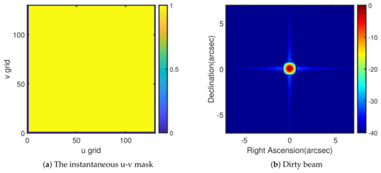
Figure 6. The instantaneous u-v mask and corresponding dirty beam.

4.4. Example 4: Extensibility

We define the filling ratio (FR) as the ratio of the number of occupied grid points (or the number of unit-valued elements in the mask $\mathbf{M}$) to the total number of grid points, $N_u{N}_v$, for evaluating the performance of uv-coverage intuitively and concisely.

In order to demonstrate the extensibility property of nested arrays, we add $\Delta N$ antennas to the second level with uniform inter-element spacing of $1.2$ km, where $\Delta N=\{0,1,2,3,4\}$. We give the variations of FR, PSL, and angular resolution of the synthesized dirty beam of the extended linear arrays in Table 1. With the number of antennas increasing, the FR of the extended linear nested arrays rises continuously, by which we can obtain more spatial frequencies from the celestial source. At the same time, the PSL of the extended linear nested arrays has a significant decline, and we can retrieve more clear source images by extended linear nested arrays. Moreover, the improvement of angular resolution performance shown in Table 1 indicates that the extended arrays have good imaging performance. The variations of FR, PSL, and angular resolution of the synthesized dirty beam of the extended linear arrays show good extensibility of the structure we proposed.

Table 1. The variations of FR (%), PSL(dB), and angular resolution (arc seconds) of the extended linear arrays.

$\mathbf{\Delta }\mathit{N}$	0	1	2	3	4
FR	63.82	69.64	70.76	71.93	72.61
PSL	−17.85	−24.55	−26.26	−26.75	−27.02
Angular resolution	0.66	0.57	0.50	0.45	0.41

In addition, we compare the performance, in terms of the FR and PSL, of the Y-shaped nested array with two other Y-shaped arrays, namely Y2 and Y3 from reference [13] to present the performance of the proposed structure. The array Y2 is optimized to possess the maximum FR in the uv-plane, whereas Y3 has been designed to exhibit the lowest PSL. In order to demonstrate the extensibility performance of nested structures, we add $\Delta N$ antennas to each arm of the existing “Y”, where $\Delta N=\{0,1,2,3,4\}$. For the Y-shaped nested array, we place additional antennas in the second level with uniform inter-element spacing of 8 km. Since both Y2 and Y3 are not structured extensible arrays, we add the new antennas in the same locations as those of the Y-shaped to guarantee identical maximum baseline. In Figure 7a, we plot the variations of FR for three different extended Y-shaped arrays with the increase in antennas. Obviously, compared with original Y-shaped arrays, the FR of arrays Y2 and Y3 has a clear decline with antennas added to each arm of “Y”. Because the added arrays make the outer of the uv-masks sparser than that of original arrays, the decline in FR can be relieved by increasing the number of antennas. In contrast, the FR of the Y-shaped nested array increases continuously with antennas added, due to which both the inner and outer of the uv-masks become denser, which indicates that the Y-shaped nested array can obtain more spatial frequencies with extension of the array, while the others show bad performance compared with initial Y-shaped arrays.

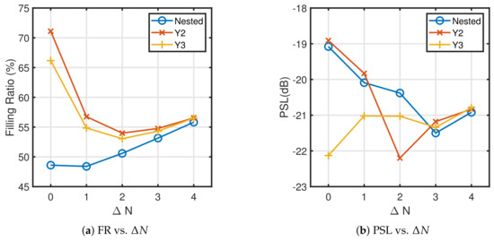
Figure 7. The variations of FR and PSL for three different extended Y-shaped arrays.

The plot of PSL vs. $\Delta N$ for the three different extended Y-shaped configurations is depicted in Figure 7b. Compared with the initial array, we can see that the PSL of array Y3 increases with antennas added and exceeds that of the Y-shaped nested array when $\Delta N=3$. Meanwhile, the PSL of array Y2 ultimately exceeds that of the Y-shaped nested array, although it has an evident decrease when only one or two antennas are added. On the contrary, the PSL of the Y-shaped nested array decreases obviously with increasing $\Delta N$, which indicates that the extended Y-shaped nested array has a good performance in PSL. In addition, due to the increase in uv aperture, the angular resolution of extended Y-shaped nested arrays performs well, as shown in Table 2, which indicates that extended Y-shaped nested arrays have good imaging performance. The variations of FR, PSL, and angular resolution of the synthesized dirty beam for three different extended Y-shaped arrays manifest the good extensibility of nested structures.

Table 2. The variation of angular resolution (arc seconds) of the extended Y-shaped nested arrays.

$\mathbf{\Delta }\mathit{N}$	0	1	2	3	4
Angular resolution	0.14	0.10	0.08	0.07	0.06

4.5. Example 5: Source Image Retrieval

Finally, we demonstrate the effectiveness of nested arrays and compare the performance of different arrays through image recovery. In order to better assess the image retrieval performance of different arrays, we utilize a 2D Gaussian source with visibility defined by

$$V(u,v)=\frac{1}{\sqrt{2\pi }\sigma }{e}^{-(u^2+v^2)/2{\sigma }^2},$$

(11)

where $\sigma$ represents standard deviation, and we set $\sigma =B_{\max }/\left(6\lambda \right)$, thereinto, $B_{\max }$ denotes the maximum baseline length in zenith observation. Note that the angular width of the original Gaussian source varies for different arrays. In Figure 8a, we plot the original image corresponding to the Y-shaped nested array with 27 antennas (i.e., $B_{\max }=21\sqrt{3}$ km) for comparison, obtained using a $512\times 512$ inverse FFT of the sampled visibilities.

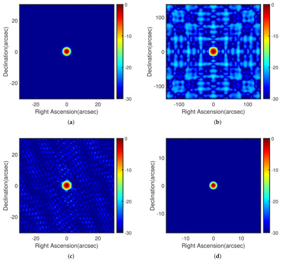
Figure 8. True 2D Gaussian source and retrieved images by different nested arrays. (a) True 2D Gaussian source for Y-shaped nested array with 27 antennas. (b) Linear nested array. (c) Y-shaped nested array. (d) 2D nested array.

Figure 8b,c,d show the source images retrieved from the uv sampling points plotted in Figure 4a, Figure 5a, and Figure 6a for the linear nested array, Y-shaped nested array, and 2D nested array, respectively. Since different arrays acquire various uv-coverages, which determine the performance of source image retrieval, we can obtain various retrieved images through different arrays. Comparing Figure 8b,c, we can find the performance of the Y-shaped nested array with 27 antennas exceeds that of the linear nested array, as the latter has a higher PSL as shown in Examples 1 and 2. Compared with the linear and Y-shaped nested arrays, we can clearly see that the 2D nested array provides superior image quality, owing to its complete uniform uv-coverage.

In Figure 9a,b, we depict source images retrieved by extended linear nested arrays. Compared with Figure 8b, it is clear that from extended linear arrays we can obtain better images, which indicates the structure we proposed has a good performance in image recovery.

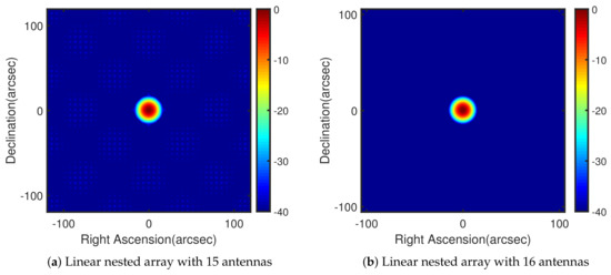
Figure 9. Retrieved images by extended linear nested arrays.

The source images retrieved by the extended Y-shaped arrays with 30 and 33 elements are shown in Figure 10a,b, respectively. Comparing Figure 8c and Figure 10a,b, because of the improvement in PSL and FR, we acquire a better uv-coverage and significant improvement in imaging performance of the Y-shaped nested arrays with increasing number of antennas, which shows the structure we proposed performs well in source image retrieval.

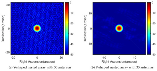
Figure 10. Retrieved images by extended Y-shaped nested arrays.

5. Conclusions

In this paper, based on nested arrays and the concept of coarray, which are applied in various fields, we designed nested interferometric array configurations, which have a good performance in extensibility using the concept of difference coarray for both supersynthesis and instantaneous modes. Nested configurations exhibit tangible advantages, including extensibility and regular lattice positions, which improves the flexibility and scalability of existing arrays. The simulation results show that the array configurations we proposed can acquire better PSL and higher FR with an increase in array elements. Furthermore, retrieved simulated celestial source images by extended arrays validated the effectiveness of the proposed array configurations. However, there are some limitations. First, we utilized $N_u=N_v=128$ grids to sample the uv-coverage, which may lead to the loss of some spatial frequencies; more grids can be used to improve this problem in later studies. Second, each grid of the uv-masks is represented as one or zero, corresponding to having uv-points fall into that grid or not. Then, the dense uv-coverage and sparse uv-coverage cannot be distinguished, and those may affect the synthesized dirty beam. Furthermore, different weighting functions also have an influence on the synthesized dirty beam.

References

- Wang, X.; Wang, P.; Chen, V.C. Simultaneous measurement of radial and transversal velocities using interferometric radar. IEEE Trans. Aerosp. Electron. Syst. 2019, 56, 3080–3098. [Google Scholar] [CrossRef]
- Xu, G.; Gao, Y.; Li, J.; Xing, M. InSAR phase denoising: A review of current technologies and future directions. IEEE Geosci. Remote Sens. Mag. 2020, 8, 64–82. [Google Scholar] [CrossRef]
- Josaitis, A.T.; Ewall-Wice, A.; Fagnoni, N.; De Lera Acedo, E. Array element coupling in radio interferometry I: A semi-analytic approach. Mon. Not. R. Astron. Soc. 2022, 514, 1804–1827. [Google Scholar] [CrossRef]
- Wang, X.; Li, W.; Chen, V.C. Hand Gesture Recognition Using Radial and Transversal Dual Micromotion Features. IEEE Trans. Aerosp. Electron. Syst. 2022, 58, 5963–5973. [Google Scholar] [CrossRef]
- Xu, G.; Zhang, B.; Yu, H.; Chen, J.; Xing, M.; Hong, W. Sparse synthetic aperture radar imaging from compressed sensing and machine learning: Theories, applications, and trends. IEEE Geosci. Remote Sens. Mag. 2022, 10, 32–69. [Google Scholar] [CrossRef]
- Viher, M.; Vuković, J.; Racetin, I. A Study of Tropospheric and Ionospheric Propagation Conditions during Differential Interferometric SAR Measurements Applied on Zagreb 22 March 2020 Earthquake. Remote Sens. 2023, 15, 701. [Google Scholar] [CrossRef]
- Su, Y.; Nan, R.; Peng, B.; Roddis, N.; Zhou, J. Optimization of interferometric array configurations by “sieving” u–v points. Astron. Astrophys. 2004, 414, 389–397. [Google Scholar] [CrossRef]
- Debary, H.; Mugnier, L.M.; Michau, V. Aperture configuration optimization for extended scene observation by an interferometric telescope. Opt. Lett. 2022, 47, 4056–4059. [Google Scholar] [CrossRef]
- Thompson, A.R.; Moran, J.M.; Swenson, G.W. Interferometry and Synthesis in Radio Astronomy; Springer: Berlin/Heidelberg, Germany, 2017. [Google Scholar]
- Cornwell, T. A novel principle for optimization of the instantaneous Fourier plane coverage of correlation arrays. IEEE Trans. Antennas Propag. 1988, 36, 1165–1167. [Google Scholar] [CrossRef]
- Kogan, L. Optimizing a large array configuration to minimize the sidelobes. IEEE Trans. Antennas Propag. 2000, 48, 1075–1078. [Google Scholar] [CrossRef]
- Mathur, N. A pseudodynamic programming technique for the design of correlator supersynthesis arrays. Radio Sci. 1969, 4, 235–244. [Google Scholar] [CrossRef]
- Jin, N.; Rahmat-Samii, Y. Analysis and particle swarm optimization of correlator antenna arrays for radio astronomy applications. IEEE Trans. Antennas Propag. 2008, 56, 1269–1279. [Google Scholar] [CrossRef]
- Oliveri, G.; Caramanica, F.; Massa, A. Hybrid ADS-based techniques for radio astronomy array design. IEEE Trans. Antennas Propag. 2011, 59, 1817–1827. [Google Scholar] [CrossRef]
- Moffet, A. Minimum-redundancy linear arrays. IEEE Trans. Antennas Propag. 1968, 16, 172–175. [Google Scholar] [CrossRef]
- Hoctor, R.T.; Kassam, S.A. Array redundancy for active line arrays. IEEE Trans. Image Process. 1996, 5, 1179–1183. [Google Scholar] [CrossRef]
- Bloom, G.S.; Golomb, S.W. Applications of numbered undirected graphs. Proc. IEEE 1977, 65, 562–570. [Google Scholar] [CrossRef]
- Vaidyanathan, P.P.; Pal, P. Sparse sensing with co-prime samplers and arrays. IEEE Trans. Signal Process. 2011, 59, 573–586. [Google Scholar] [CrossRef]
- Pal, P.; Vaidyanathan, P.P. Nested arrays: A novel approach to array processing with enhanced degrees of freedom. IEEE Trans. Signal Process. 2010, 58, 4167–4181. [Google Scholar] [CrossRef]
- Liu, J.; Zhang, Y.; Lu, Y.; Ren, S.; Cao, S. Augmented nested arrays with enhanced DOF and reduced mutual coupling. IEEE Trans. Signal Process. 2017, 65, 5549–5563. [Google Scholar] [CrossRef]
- Liu, S.; Mao, Z.; Zhang, Y.D.; Huang, Y. Rank minimization-based Toeplitz reconstruction for DoA estimation using coprime array. IEEE Commun. Lett. 2021, 25, 2265–2269. [Google Scholar] [CrossRef]
- Hoctor, R.T.; Kassam, S.A. The unifying role of the coarray in aperture synthesis for coherent and incoherent imaging. Proc. IEEE 1990, 78, 735–752. [Google Scholar] [CrossRef]
- Chow, Y. On designing a supersynthesis antenna array. IEEE Trans. Antennas Propag. 1972, 20, 30–35. [Google Scholar] [CrossRef]
- Van der Veen, A.J.; Leshem, A.; Boonstra, A.J. Signal processing for radio astronomical arrays. In Proceedings of the Processing Workshop Proceedings, 2004 Sensor Array and Multichannel Signal, Barcelona, Spain, 18–21 July 2004; IEEE: Piscataway, NJ, USA, 2004; pp. 1–10. [Google Scholar]
- Bracewell, R. Optimum spacings for radio telescopes with unfilled apertures. Natl. Acad. Sci. Natl. Res. Council. Publ. 1966, 1408, 243–244. [Google Scholar]
- Napier, P.J.; Thompson, A.R.; Ekers, R.D. The very large array: Design and performance of a modern synthesis radio telescope. Proc. IEEE 1983, 71, 1295–1320. [Google Scholar] [CrossRef]
- Pal, P.; Vaidyanathan, P.P. Nested arrays in two dimensions, Part I: Geometrical considerations. IEEE Trans. Signal Process. 2012, 60, 4694–4705. [Google Scholar] [CrossRef]
- Karastergiou, A.; Neri, R.; Gurwell, M.A. Adapting and expanding interferometric arrays. Strophys. J. Suppl. Ser. 2006, 164, 552–558. [Google Scholar] [CrossRef]
Disclaimer/Publisher’s Note: The statements, opinions and data contained in all publications are solely those of the individual author(s) and contributor(s) and not of MDPI and/or the editor(s). MDPI and/or the editor(s) disclaim responsibility for any injury to people or property resulting from any ideas, methods, instructions or products referred to in the content. |
© 2023 by the authors. Licensee MDPI, Basel, Switzerland. This article is an open access article distributed under the terms and conditions of the Creative Commons Attribution (CC BY) license (https://creativecommons.org/licenses/by/4.0/).