2D&3DHNet for 3D Object Classification in LiDAR Point Cloud

Abstract

Accurate semantic analysis of LiDAR point clouds enables the interaction between intelligent vehicles and the real environment. This paper proposes a hybrid 2D and 3D Hough Net by combining 3D global Hough features and 2D local Hough features with a classification deep learning network. Firstly, the 3D object point clouds are mapped into the 3D Hough space to extract the global Hough features. The generated global Hough features are input into the 3D convolutional neural network for training global features. Furthermore, a multi-scale critical point sampling method is designed to extract critical points in the 2D views projected from the point clouds to reduce the computation of redundant points. To extract local features, a grid-based dynamic nearest neighbors algorithm is designed by searching the neighbors of the critical points. Finally, the two networks are connected to the full connection layer, which is input into fully connected layers for object classification.

1. Introduction

Intelligent vehicles ensure safe driving through environmental perception and autonomous control technologies, which improve global and local navigation efficiency [1]. Light Detection and Ranging (LiDAR) sensors have the advantages of high scanning accuracy, long-distance measurement, high resolution, and high stability. LiDAR remote sensing technologies capture high-precision object structure and terrain elevation for environment perception tasks [2,3]. Currently, the semantic map generation technologies in LiDAR point clouds are widely used in unmanned vehicle perception systems such as Google, Baidu Apollo, Boss, Junior, etc., and become hotspots of unmanned driving [4].

LiDAR point clouds have the characteristics of unstructured distribution, uneven density, and sparse distribution. Additionally, LiDAR scans surface points from certain angles of a 3D object, so that the reverse side cannot be observed. Thus, 3D object classification of LiDAR point clouds becomes a challenging problem, which has been researched from traditional machine learning methods to deep network models. Machine learning research based on the geometric characteristics of 3D point clouds is suitable for the segmentation task in a limited scanning range. Because the close-range LiDAR point cloud is dense, and the distant point cloud is loose, the machine learning method has problems of insufficient adaptability and poor expansion ability [5]. Deep neural networks have achieved remarkable performance in object recognition for the 2D image and video streams. However, when applied to the unstructured and irregular LiDAR point clouds, the traditional neural networks have difficulty processing the point cloud directly. By mapping 3D point clouds to multiple views, the deep learning modules for processing 2D images can be reused. This methodology converts the high-precision LiDAR data to rasterized pixels, which causes original accuracy loss. To process the irregular point clouds directly, some researchers apply multi-layer perceptron (MLP) and a maximum pooling layer to extract the global features of the point cloud and combine the multi-scale local features [6].

In this paper, we propose a hybrid 2D and 3D Hough Net (2D&3DHNet) for 3D object classification, which combines global and local Hough features with a deep learning model. Firstly, each 3D point is mapped to a series of cells of 3D Hough space by a 3D Hough transform algorithm [7]. All the cells are accumulated with the value of the casting votes. Then, we utilize hybrid analysis mechanisms of 3D global features and 2D local features for accurate object classification. The global Hough features are generated from the Hough space and input into a 3D convolutional neural network (CNN) for training global features. To remove redundant points and retain the local spatial structure of the object, a multi-scale critical point sampling method is designed to extract critical points in the 2D views projected from the point clouds. In the local features extraction process, a grid-based dynamic nearest neighbors algorithm is designed to quickly search the neighboring points nearby the extracted critical points. The 2D Hough features are calculated based on the sampled neighboring points of each critical point, which are combined into a local Hough feature map. The local features are extracted by a 2D CNN implemented on the local Hough features. Finally, the two networks are connected and input into the fully connected layers for object classification. After several iterative training processes, the proposed method achieves high classification accuracy.

The main contributions of this paper are as follows:

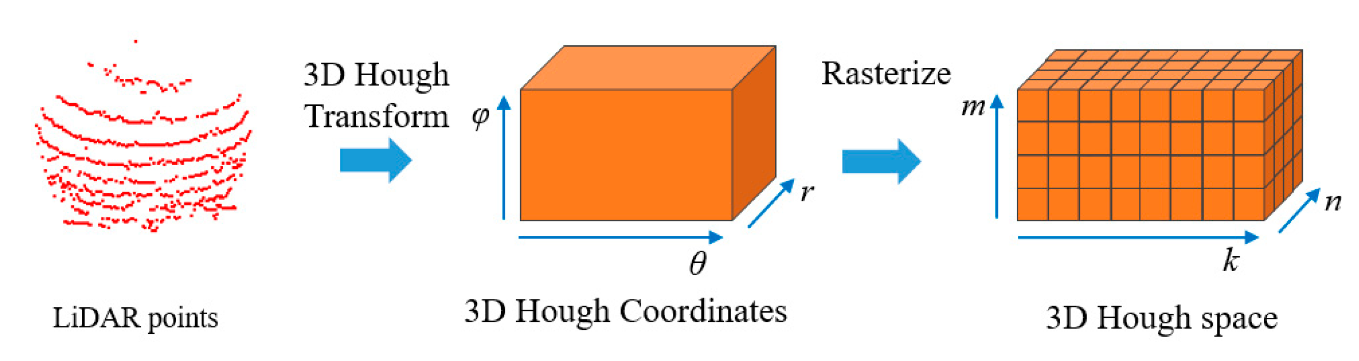
• Each cell in the 3D Hough space voted by the relevant numerous coplanar points represents the normal vector of their plane as a common feature. Thus, the Hough descriptors have a wide effective receptive field. The Hough features are voted by a set of unordered coplanar points, which satisfies the permutation invariant requirement of deep neural networks. Furthermore, the extracted planar features are stable against the point loss and non-uniform density of LiDAR point clouds.
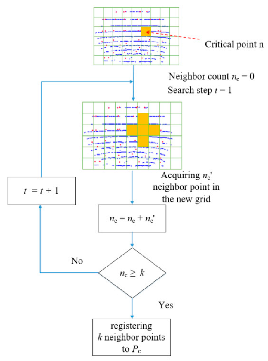
• The multi-scale critical point sampling method is developed to extract critical points for retaining the local spatial structure of the object. This way, the redundant points are removed to reduce the local features computation time cost.
• To preserve the local features, the grid-based dynamic nearest neighbors algorithm is developed to select a certain number of points nearby the critical points for discrimination of local features generation.
• The fusion of 3D global and 2D local Hough features enables discriminative structure retrieval and improves classification accuracy.

This paper is organized as follows: Section 2 investigates related works about LiDAR point cloud processing methods and object classification models. Section 3 describes the 3DHNet for 3D object classification. Section 4 describes our experimental platform and object classification results. Section 5 provides a summary of this paper.

2. Related Works

Currently, autonomous vehicles with environment perception and remote sensing technologies are widely researched for intelligent traffic. To explore the impact of autonomous driving technology on sustainable urbanization development, Acheampong et al. [8] applied a set of theory-grounded and behaviorally realistic models to understand public attitudes and preferences for autonomous vehicles. Dowling et al. [9] verified the shaping effect of autonomous driving technology on urban material, and political and economic structures through different experiments. In addition, the emerging technology of autonomous driving has promoted the development of smart cities and made urban governance more intelligent [10]. Petrović et al. [11] analyzed the communication efficiency between autonomous vehicles and drivers for reducing the incidence of traffic accidents. In the field of autonomous driving technology, LiDAR point clouds play an important role in unknown environment modeling and perception for behavior planning of autonomous driving.

The 3D object classification algorithms based on machine learning mechanisms, such as random forest, support vector machine, and AdaBoost, extract the global or local features of the point cloud object as discriminative information [12,13,14]. However, the distribution of LiDAR point clouds is dense in the near field and loose in the far field. The machine learning methods analyze the extracted features through prior knowledge, which causes poor generalization and expansion ability, especially for occlusion and overlap situations [15].

Deep neural networks have made remarkable achievements in the application of semantic segmentation and object recognition in the 2D image and video streams. Because a LiDAR point cloud dataset has the characteristics of an irregular distribution and unstructured data structure, it is difficult for the deep learning models to process the LiDAR point clouds directly.

Su et al. [16] proposed a multi-view CNN for 3D shape recognition by capturing 3D virtual objects from different viewports to obtain multiple 2D projection images as the input of the CNN classification model. Feng et al. [17] proposed an object shape recognition CNN model with a view–group–shape architecture. From multiple projection views of the 3D object, the view-level descriptors were extracted using a fully convolutional network and a CNN framework. In the process of view-level pooling, this method combines grouping information to represent shape features, which significantly improves classification performance. In the other multi-view classification networks, such as the multi-view coordinated bilinear network [18], LU-Net model [19], and 3D-MiniNet [20], the mapping process from 3D points to 2D view caused accuracy loss of high-precision original data and local features, which resulted in inaccurate classification. Additionally, a large number of hyperparameters need to be manually adjusted for feature extraction.

Maturana [21] proposed a VoxNet by registering point clouds into a structured 3D voxel model, which was input into a 3D CNN. This method satisfied the CNN input requirement of the unified data structure without losing much geometric spatial information. C. Wang et al. [22] proposed a NormalNet network integrating object voxel features and surface normal vector information. Compared with VoxNet, the object recognition performance of the NormalNet was greatly improved. However, the voxel-based deep neural networks caused high space and time complexity.

To reverse local features, Le et al. [23] proposed a PointGrid model, which used a point quantization strategy to extract the same count of points in each cell grid to easily extract local geometric features. Compared with the voxel models, PointGrid had better scalability and avoided information loss. However, the sparse feature of the LiDAR point clouds caused a large number of empty data in the allocated grid, resulting in unnecessary computation [24]. If the resolution was reduced, the classification accuracy decreased. The high resolution led to high computation. In addition, the maximum resolution of the voxel model was limited by the model training capability.

To process the unordered 3D points directly, point-based deep learning algorithms were proposed, such as PointNet and Pointwise-CNN [25]. These methods only considered global point features without local geometry information. Qi et al. [26] proposed PointNet++ as a follow-up work of PointNet, which grouped point clouds into several regions and computed the local features by implementing PointNet in each region. To extract local detail features with low computing costs, PointNet++ utilized the farthest point sampling method to extract critical points of point cloud objects. Wang et al. [27] proposed a spatial pooling deep neural network (DNNSP). For each point, an 18-dimensional feature vector was calculated through its K neighboring points. Each vector contained 6-dimensional eigenvalue features and 12-dimensional Spin Image features, with K being 30, 60, and 90 respectively, to obtain the 54-dimensional feature vector as the input of DNNSP. To ensure the constancy of the point cloud, the network learned the features of each point through the weighted shared MLP layer. However, the LiDAR characteristics of radial density variation caused high time complexity of neighboring points sampling and ineffective local feature learning for the sparse point distribution in far regions.

Hough transform was always used to detect lines and planes in computer vision and image processing [28]. To extract road information from highly complex urban scenes, Hu et al. [29] adopted an iterative Hough transform algorithm to detect candidate road fringes. To detect the 3D roof plane of buildings, Tarsha-Kurdi et al. [30] applied the 3D Hough transform algorithm to extract the optimal plane from the 3D building point clouds. Sampath et al. [31] analyzed the surface normals from LiDAR point clouds to segment and reconstruct the roof surfaces of the polyhedral building. In the field of remote sensing, Xue et al. [32] proposed a derivative-free optimization algorithm to detect architectural symmetry in 3D point clouds. To accurately retrieve individual trees and crown attributes, Leeuwen et al. [33] applied the Hough transform algorithm to establish a new canopy model by fitting simple geometric shapes. Widyaningrum et al. [34] proposed an ordered points-aided Hough transform (OHT) to extract building outlines from point clouds.

Some researchers have conducted semantic analysis from Hough space. K. Zhao et al. [35] proposed an end-to-end semantic line detection framework by combining the classical Hough transform with deep learning. The depth representation extracted by the neural network was transformed from feature space to parameter space by the Hough transform. By filtering the peak value in parameter space, the semantic lines were detected efficiently. To find the centroid of 3D objects of LiDAR point clouds, C. Qi et al. [36] proposed a VoteNet, an end-to-end 3D object detection network. Referring to Hough’s voting mechanism, the object centroid point was generated through Hough voting. To refer the Hough transforming method in the 3D object classification task, we proposed a 3D object classification method based on CNN and Hough space [37]. The point clouds were projected to the X–Z plane. The Hough features generated from the projected points were input into the CNN to train the object classification model. Due to the loss of spatial structure information of the point cloud by 2D projection, this paper applied the 3D Hough transform algorithm with the critical point sampling method to improve the accuracy and efficiency of object classification.

This paper applies Hough features generated from the LiDAR point clouds of the 3D objects as the input of a deep learning model for object classification, which can resist the interference of outliers and solve the problem of disequilibrium of point cloud density.

3. Object Recognition Method

Figure 1 presents the 2D&3DHNet framework for 3D object classification in LiDAR point clouds. The proposed 2D&3DHNet applies 3D CNN and 2D CNN to extract high-dimension global and local features, respectively, and fully connected layers to realize the fusion of global and local features.

Figure 1. The framework of 2D&3DHNet for object classification in LiDAR point clouds.

3.1. Global Hough Features Extraction

The 3D Hough transform algorithm is applied to convert the 3D point clouds to the 3D Hough space, based on the coordinate transformation principle between the 3D Cartesian coordinate system and polar coordinate system, formulated as (1) [7]. For each point p(x, y, z), a serial of vectors (θ, φ, r) are calculated as Hough coordinates, where variables θ ∈ [0, 2π] and φ ∈ [0, π] are sampled with a certain step.

$$r=x\sin \left(\theta \right)\cos \left(\phi \right)+y\sin \left(\theta \right)\sin \left(\phi \right)+z\cos \left(\theta \right)$$

(1)

As shown in Figure 2, a Hough space H is combined by I × J × K rasterized cells h(i, j, k). The variable h(i, j, k) is accumulatively voted by the mapped Hough coordinates in the cell (i, j, k). The high value of h(i, j, k) means that many coplanar points exist in the plane (θ(i), φ(j), r(k)). After all point clouds are converted and registered into the Hough space, the global Hough features of the 3D objects are extracted as the variables in the Hough space.

Figure 2. The 3D Hough space generation process.

3.2. Local Hough Feature Generation

To retain the local spatial structure of point clouds and topological geometry information, a multi-scale critical point sampling method is designed to extract critical points, and a dynamic nearest neighbor sampling method is developed to select neighboring points surrounding the critical points for local features generation.

LiDAR scanning datasets contain a large number of points that causes the high memory and time complexity for generating local features. To compute the discriminative geometric structure with a small number of points, a multi-scale critical point sampling method is developed to select critical points in all the valid grids of the 2D view projected from the point clouds. Figure 3 illustrates the process of searching n critical points from the object point cloud of uncertain counts and non-uniformed structure. Firstly, the point cloud is mapped to h × w grids. In each grid, the point closest to the center point of the grid is considered as the critical point. By traversing all the valid grids, m critical points are registered in the critical point list n’. If the point count in the critical point list is less than the target number n, m critical points are temporarily stored in the critical point list c. Then, the grid resolution is scaled by s. The critical point sampling process is iteratively implemented from the new scaling grid until the number of critical points list n’ is greater than or equal to the target number n. Finally, n critical points are sampled by combining the down-sampled critical point lists.

Figure 3. The process of multi-scale critical point sampling.

For extracting local features from LiDAR point clouds of uneven density, the grid-based dynamic nearest neighbor algorithm is developed to choose the nearest neighboring points surrounding the 2D critical points with low computing complexity. Figure 4 illustrates the process of searching k nearest neighboring points from the points in the local neighboring grids of a critical point. For each critical point n, the neighbor points are searched in its neighbor grids. If the sampled neighbor count n_c is smaller than k, the search grid range t is increased by 1 step. The neighboring grids propagate outward until the count of registered neighbors is equal to k.

Figure 4. The grid-based dynamic nearest neighbors algorithm.

Using the 2D Hough transform, the k neighboring points sampled for a critical point are mapped into a 2D local Hough space, which contains M × N elements. As shown in Figure 5, after n × k feature points are obtained, the Hough transform is performed on k nearest neighbor points around each key point n. Thus, n groups of Hough spaces are obtained and rasterized into n groups of M × N grids. Then the elements in each feature group are expanded into 1 dimension of M × N grids. Finally, a 2D feature map the size of n × (M × N) is obtained by merging n groups of tiled grids to obtain a 2D local feature map.

Figure 5. The 2D local feature generation process from the critical points’ neighbors.

3.3. 2D&3DHNet

The proposed 2D&3DHNet framework is shown in Figure 2. The generated 3D global Hough features of I × J × K dimensions are input into the 3D global feature extraction network. In the following 3D CNN, several different 3D convolution kernels are performed by sliding on the data spaces. The padding type is set to “SAME” to ensure that the input size is the same as the output size. The ReLU activation function max(0, x) is used to avoid the vanishing gradient problem. Between the convolutional layers, the 3D max-pooling is performed for spatial downsampling.

The generated 2D local Hough features of I’ × J’ dimensions are input into the 2D local feature extraction network. In the 2D CNN, several 1D convolution kernels are operated on the previous layer. Additionally, the padding is set to SAME, the ReLU activation function max(0, x) is used, and the 2D max-pooling is performed for spatial downsampling.

The global and local features extracted by the 2D CNN and 3D CNN are flattened to 1D spaces of I × J × K × 16 and I’ × J’ × 8, which combine as the input of the fully connected layers as the classification network. The neuron counts of the hidden layers are 1024, 512, 128, and 64, respectively. Using the softmax function, the outputs of the fully connected layers are transformed into values between 0 and 1. The node corresponding to the maximum value is the predicted label.

During the backpropagation process, the cross-entropy function is applied as the loss function. The gradient descent method is used to update the weight and deviation parameters of the deep neural networks. After the iterative training processes, the 2D&3DHNet model is optimized.

4. Experiments

4.1. Experimental Environment

Experiments in this section were conducted using an Intel^® Xeon^® CPU E5-2670 v3 @ 2.30 GHz × 2 dual processor (Intel, Santa Clara, CA USA), an NVIDIA Quadro K5200 graphics card (NVIDIA, Santa Clara, CA USA), and 16 GB RAM (Micron, Boise, ID, USA).

We developed a semi-automatic 3D object labeling tool to segment LiDAR point clouds into separate objects and generated a 3D object dataset in our previous work [37]. The objects of 6 types were collected in our dataset, including poles, pedestrians, trees, bush, buildings, and vehicles. We selected 1332 samples from our dataset and a part of samples from the Sydney Urban object dataset (NSW, AUS) [38] to combine into the training and evaluation datasets, detailed in Table 1.

Table 1. LiDAR point cloud object classification training and testing dataset.

Category	Sydney	Our	Training Dataset	Evaluation Dataset	Total
pole	0	236	160	76	236
pedestrian	69	83	92	60	152
tree	0	415	286	129	415
bush	0	223	141	82	223
building	0	385	252	133	385
vehicle	97	93	115	75	190
Total	166	1435	1046	555	1601

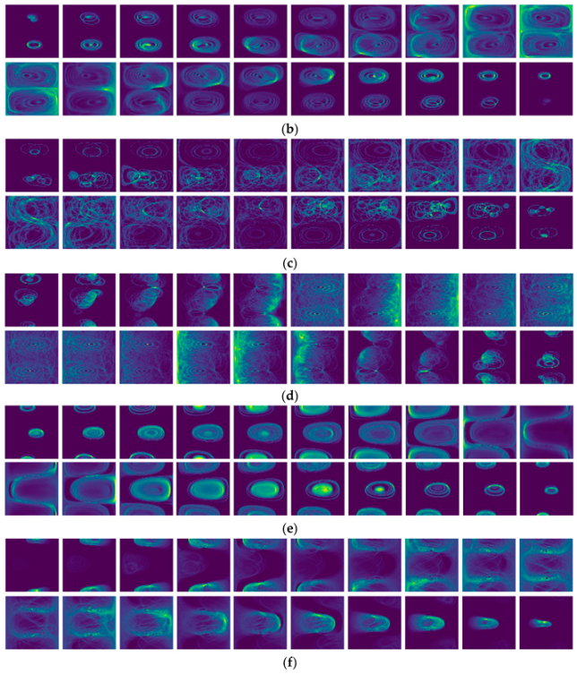
4.2. Global Hough Feature Analysis

Figure 6 visualizes some of the 2D slices (i, k) sampled from the 3D Hough spaces of 6 objects with I = J = K = 80. From left to right images, the j value increased by 4 steps. When the corresponding variable φ(j) increased to the median value, the Hough slices became discriminative between each other.

Figure 6. The 3D Hough spaces mapped from 6 samples of different objects: (a) pole, (b) pedestrian, (c) tree, (d) bush, (e) building, (f) vehicle.

Figure 6 illustrates that the 3D Hough spaces of pole and pedestrian were similar, because these objects had a cylinder shape distribution. However, the Hough space density of pedestrians was sparser on the side and higher in the middle compared with that of the pole. Figure 6d indicates the Hough space of the bush object, whose density was highest in the middle. Figure 6e shows the Hough spaces of the buildings, which were similar to the pole and pedestrian in the middle part, but discriminative on the side. The Hough spaces of bush and vehicle objects were easy to distinguish from other objects.

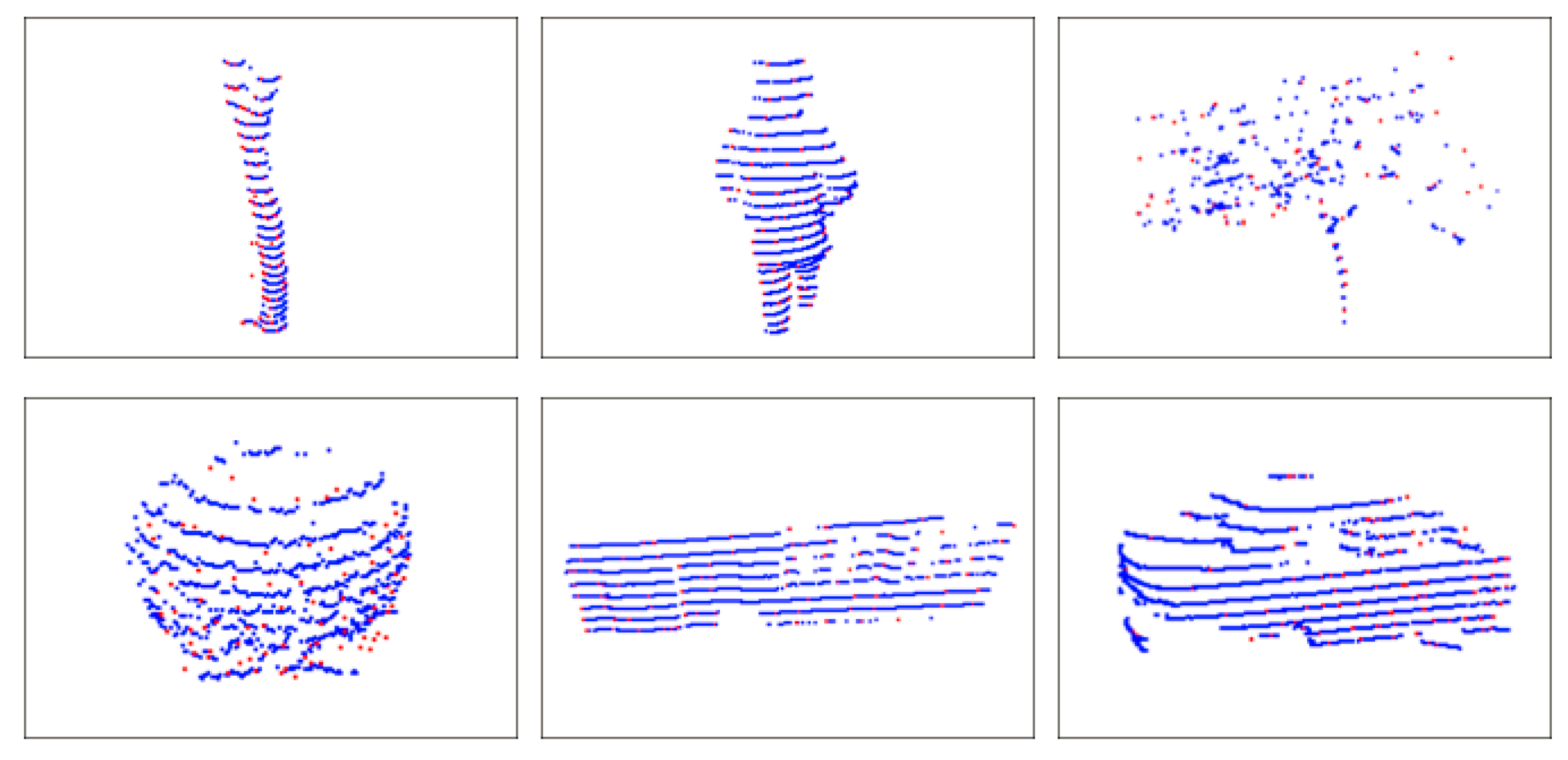
4.3. Local Hough Feature Analysis

Figure 7 shows some critical points selecting results using the multi-scale critical point sampling method, where the critical points were rendered in red. We initialized the sampling method with the grid parameter h = w = 10, the scale variable s = 0.8, and m = 100 critical points as the sampling target. After three looping operations, 100 critical points were sampled, which were distributed evenly inside the object surface and retained the object details within a few valuable data.

Figure 7. The critical point selection examples generated by the multi-scale critical point sampling method.

Figure 8a compares the average time consumption of the farthest point sampling (FPS) and our multi-scale critical point sampling methods implemented on the 6 kinds of objects. The critical points sampling time of our method was 1.455 s on average, around one-third of the FPS time consumption. Figure 8b compares the average time consumption of the K nearest neighbor point (KNN) sampling method and our grid-based dynamic nearest neighbors algorithm. The neighbor points sampling time of our method was 1.013 s on average, much less than that of the KNN method.

Figure 8. Time consumption comparison of critical points and neighbor points sampling: (a) critical points sampling, (b) nearest neighbors sampling.

Figure 9 visualizes the 2D local Hough spaces of 6 objects, which were initialized with m = 100 critical points and k = 10 neighbor points for each critical point. The local Hough spaces of pole and bush were evenly distributed, while the density of the pole was higher than that of the bush. The local Hough spaces of pedestrians, trees, and buildings formed like cylindrical spaces and were distinguished from each other. In addition, the local Hough features of vehicles concentrated on the upper, middle, and lower regions.

Figure 9. Examples of the 2D local Hough spaces generated from 6 object samples: (a) pole, (b) pedestrian, (c) tree, (d) bush, (e) building, (f) vehicle.

4.4. Classification Performance Using Global Hough Features

This section tested the classification performance only using global Hough features with different resolutions of 20 × 20 × 20, 25 × 25 × 25, 30 × 30 × 30, and 32 × 32 × 32. The 3D global feature extraction network was performed by three 3D convolution layers with 64 1 × 1 × 1 convolution kernels, four 2 × 2 × 2 max-pooling layers, and four FC layers with 512, 256, 128, and 64 neurons, as well as the output layer with 6 output values.

Table 2 indicates the object classification performances with different resolutions of Hough spaces. We counted the true positive (TP), false negative (FN), false positive (FP), and true negative (TN) samples of the classification results. To evaluate the classification performance, the precision (P), recall (R), F1 scores, and accuracy were calculated by using Equations (2)–(5), respectively. When the resolution was 25 × 25 × 25, the average F1 score and classification accuracy were 95.3% and 95.7%, respectively. Because of the diverse distribution and a few car samples, the F1 score of the vehicle category was 90.6%, not as high as the others.

$$P=\frac{TP}{TP+FP}$$

(2)

$$R=\frac{TP}{TP+FN}$$

(3)

$$F1=2\times \frac{P\times R}{P+R}$$

(4)

$$Accuracy=\frac{TP+TN}{TP+TN+FP+FN}$$

(5)

Table 2. Classification performance of the six objects with different resolutions of Hough spaces.

Type	20 × 20 × 20			25 × 25 × 25			30 × 30 × 30			32 × 32 × 32
	P	R	F1	P	R	F1	P	R	F1	P	R	F1
pole	94.9%	97.4%	96.1%	95%	100%	97.4%	100%	98.7%	99.3%	90.5%	100%	95%
pedestrian	100%	78.3%	86.8%	96.4%	90%	93.1%	94.2%	81.7%	87.5%	100%	76.7%	86.8%
tree	87.5%	98.4%	92.6%	94.7%	96.9%	95.8%	93.9%	96.9%	95.4%	93.2%	95.4%	94.3%
bush	95.2%	97.6%	96.4%	96.5%	100%	98.2%	91.9%	96.3%	94.%	90.1%	100%	94.8%
building	94.9%	98.5%	96.7%	94.3%	99.2%	96.7%	97%	98.5%	97.8%	95.6%	98.5%	97%
vehicle	96.8%	81.3%	88.4%	100%	82.7%	90.6%	89.2%	88%	88.6%	95.4%	82.7%	88.6%
Avg	94.8%	91.9%	92.8%	96.4%	94.8%	95.3%	94.3%	93.3%	93.7%	94.1%	92.2%	92.7%
Accuracy	93.5%			95.7%			94.6			93.7

Bold indicates that at the current resolution, this indicator is the best.

Figure 10 shows the confusion matrix of classification results. The pedestrian objects were easily recognized as trees at the resolutions of 20 × 20 × 20, 25 × 25 × 25, 30 × 30 × 30, and 32 × 32 × 32. Furthermore, the vehicles were recognized as trees and bush objects, because their global spatial distributions were similar to each other. Thus, the classification needed to be optimized based on the local information.

Figure 10. Classification confusion matrix for 6 kinds of object point clouds with different resolutions: (a) 20 × 20 × 20, (b) 25 × 25 × 25, (c) 30 × 30 × 30, (d) 32 × 32 × 32.

4.5. Classification Performance of 2D&3DHNet

To solve the misclassification problem of pedestrian and vehicle objects, the proposed 2D&3DHNet combined with the local Hough feature information was tested. Table 3 illustrates the processing speeds for different resolutions of 3DHough spaces. In 2D local Hough space, the average time for Hough transformation was less than 0.5 s. The training time and testing time of 2D&3DHNet increased with the resolution increment. We applied GPU programming technologies to speed up the calculation of the 3D Hough transform [7], which reduced the average time of the Hough space generation process from 3 s to 0.03 s. The classification performances are detailed in Table 4, where the parameters of the 3D global Hough spaces were specified as 20 × 20 × 20, 25 × 25 × 25, and 30 × 30 × 30, and the resolution of the 2D local Hough space was specified as 0.10, 0.15, 0.20, 0.25, and 0.30. From the experimental results, when the 3D Hough resolution was 25 × 25 × 25 and the unit size of 2D Hough space was 0.25, the classification accuracy achieved 97.6% as the best performance. The classification accuracy of pole and bush was kept at 100%. The accuracy of vehicle classification was 92.0%, which was 9.3% higher than the 82.7% obtained by only using global Hough features. The accuracy of pedestrian classification was also greatly improved and achieved 96.7%. In addition, when the parameters were specified as 20 × 20 × 20 and the resolution was 0.10 and 0.25, the average classification accuracy improved to 96.67% and 96.73% respectively. When the parameter was 30 × 30 × 30 and the resolution was 0.15, the average classification accuracy was 96.6%, and the classification accuracy of pedestrians achieved 98.3%, which was 16.6% higher than with using global Hough features only.

Table 3. Processing speeds for different Hough space resolutions.

Computational Load	20 × 20 × 20	25 × 25 × 25	30 × 30 × 30	32 × 32 × 32
3D Hough transformation	1.7 s	2.7 s	3.8 s	4.3 s
Average training time (s)	170 s	173 s	176 s	178 s
Average testing time (s)	5 s	8 s	11 s	13 s

Table 4. Classification performance of the 2D&3DHNet.

I × J × K	2D Res	Pole	Pedestrian	Tree	Bush	Building	Vehicle	Avg
20 × 20 × 20	0.10	97.4%	95.0%	96.9%	100%	100%	90.7%	96.67%
	0.15	96.1%	96.7%	97.7%	98.8%	97.7%	85.3%	95.38%
	0.20	98.7%	96.7%	98.4%	100%	99.2%	86.7%	96.62%
	0.25	98.7%	96.7%	100%	100%	97.0%	88.0%	96.73%
	0.30	100%	95.0%	98.4%	100%	100%	84.0%	96.23%
25 × 25 × 25	0.10	100%	95.0%	95.3%	100%	91.0%	89.3%	95.10%
	0.15	100%	100%	97.7%	100%	93.2%	86.7%	96.27%
	0.20	100%	95.0%	95.3%	100%	97.7%	86.7%	95.78%
	0.25	100%	96.7%	99.2%	100%	97.7%	92.0%	97.60%
	0.30	100%	93.3%	95.3%	98.8%	95.5%	89.3%	95.37%
30 × 30 × 30	0.10	100%	93.3%	94.6%	97.6%	91.0%	89.3%	94.30%
	0.15	100%	98.3%	96.9%	100%	97.7%	86.7%	96.60%
	0.20	100%	90.0%	89.1%	100%	97.7%	89.3%	94.35%
	0.25	97.3%	98.3%	94.6%	100%	97.0%	88.0%	95.87%
	0.30	97.4%	96.7%	96.1%	98.8%	99.2%	85.3%	95.58%

Figure 11 shows the classification confusion matrix of 2D&3DHNet, where the parameters of the 3D Hough spaces were specified as 20 × 20 × 20, 25 × 25 × 25, and 30 × 30 × 30, and the resolution of the 2D local Hough spaces was specified as 0.25. Compared with the classification results by only using global Hough features, the misclassification ratio of pedestrians and vehicles was greatly reduced. When the global Hough space was divided into 25 × 25 × 25 grids, the classification results of the proposed 2D&3DHNet achieved the best performance.

Figure 11. Classification confusion matrix for the experiments using 2D&3DHNet: (a) 20 × 20 × 20, (b) 25 × 25 × 25, (c) 30 × 30 × 30.

4.6. Algorithms Comparison

As shown in Table 5, we compared our proposed 2D&3DHNet with the classical deep neural network models, including VoxNet [21], MVCNN [16], 3DShapeNet [39], DGCNN [40], and PointCNN [41]. The “M” stands for millions. The voxel-based classification networks, such as the VoxNet model and 3DShapeNet model, rasterized the points into structured voxels that caused the precision loss of the original data. Their average classification accuracy was around 91.7% and 93.6%, respectively. The MVCNN model input multi-view features into the CNN, which improved the classification accuracy to 95.7%. The DGCNN model extracted the local and global features of the object point cloud as the input of the network, whose classification accuracy achieved 95.3%. The PointCNN model proposed the X-transform algorithm to solve the permutation invariant problem so that the accuracy was improved to 96.2%. Experimental results show that compared with these algorithms, the proposed algorithm combining global and local Hough features for point cloud object classification had better classification performance than these deep learning methods.

Table 5. Recognition performances of 2D&3DHNet compared with other deep learning models.

Method	Input	Average Training Time (s)	Average Testing Time (s)	Accuracy	Params
VoxNet [21]	Voxel	100 s	3.5 s	91.7%	11.18M
3DShapeNet [39]	Voxel	425 s	2 s	93.6%	15.9M
MVCNN [16]	Image	2150 s	45 s	95.7%	0.92M
DGCNN [40]	Graph	8400 s	25 s	95.3%	1.35M
PointCNN [41]	point	10,750 s	30 s	96.2%	0.3M
2D&3DHNet (ours, 25 × 25 × 25 voxel)	point	147 s	9 s	97.6%	7.97M

5. Conclusions

In this paper, we proposed a 2D&3DHNet model for object classification from LiDAR point clouds. The global Hough descriptors generated from all of the object points were stable against the non-uniform density of LiDAR point clouds and had a wide effective receptive field. The local Hough features were generated based on the neighbor points nearby the critical points, which were sampled by the multi-scale critical point sampling method and the grid-based dynamic nearest neighbors algorithm. Based on the Hough spaces, the 2D&3DHNet model introduced the 3D CNN and 2D CNN to extract high-dimension global and local features, respectively, and fully connected layers to realize the fusion of global and local features. We tested the proposed method on the hybrid datasets of the Sydney Urban object dataset and ours. The experiments show that the classification accuracy achieved 97.6% by allocating the 25 × 25 × 25 cells for the 3D Hough spaces and specifying 0.25 as the unit size of the local Hough spaces. The fusion of global and local Hough spaces provides discriminative and structural features for generating available deep neural network models, which enable effective environment perception tasks of robots and intelligent vehicles.

References

1. Yan, F.; Wang, J.; He, G.; Chang, H.; Zhuang, Y. Sparse semantic map building and relocalization for UGV using 3D point clouds in outdoor environments. Neurocomputing 2020, 400, 333–342. [Google Scholar] [CrossRef]
2. Eitel, J.U.; Höfle, B.; Vierling, L.A.; Abellán, A.; Asner, G.P.; Deems, J.S.; Glennie, C.L.; Joerg, P.C.; LeWinter, A.L.; Magney, T.S.; et al. Beyond 3-D: The new spectrum of lidar applications for earth and ecological sciences. Remote Sens. Environ. 2016, 186, 372–392. [Google Scholar] [CrossRef] [Green Version]
3. Eagleston, H.; Marion, J.L. Application of airborne LiDAR and GIS in modeling trail erosion along the Appalachian Trail in New Hampshire, USA. Landsc. Urban Plan. 2020, 198, 103765. [Google Scholar] [CrossRef]
4. Li, J.; Xu, Y.; Macrander, H.; Atkinson, L.; Thomas, T.; Lopez, M.A. GPU-based lightweight parallel processing toolset for LiDAR data for terrain analysis. Environ. Model. Softw. 2019, 117, 55–68. [Google Scholar] [CrossRef]
5. Weinmann, M.; Jutzi, B.; Hinz, S.; Mallet, C. Semantic point cloud interpretation based on optimal neighborhoods, relevant features and efficient classifiers. ISPRS J. Photogramm. Remote Sens. 2015, 105, 286–304. [Google Scholar] [CrossRef]
6. Charles, R.Q.; Su, H.; Kaichun, M.; Guibas, L.J. PointNet: Deep learning on point sets for 3D classification and segmentation. In Proceedings of the 2017 IEEE Conference on Computer Vision and Pattern Recognition (CVPR), Honolulu, HI, USA, 21–26 July 2017; pp. 77–85. [Google Scholar]
7. Tian, Y.; Song, W.; Chen, L.; Sung, Y.; Kwak, J.; Sun, S. Fast Planar Detection System Using a GPU-Based 3D Hough Transform for LiDAR Point Clouds. Appl. Sci. 2020, 10, 1744. [Google Scholar] [CrossRef] [Green Version]
8. Acheampong, R.A.; Cugurullo, F.; Gueriau, M.; Dusparic, I. Can autonomous vehicles enable sustainable mobility in future cities? Insights and policy challenges from user preferences over different urban transport options. Cities 2021, 112, 103134. [Google Scholar] [CrossRef]
9. Dowling, R.; McGuirk, P. Autonomous vehicle experiments and the city. Urban Geogr. 2022, 43, 409–426. [Google Scholar] [CrossRef]
10. Cugurullo, F. Urban artificial intelligence: From automation to autonomy in the smart city. Front. Sustain. Cities 2020, 2, 38. [Google Scholar] [CrossRef]
11. Petrović, Đ.; Mijailović, R.; Pešić, D. Traffic accidents with autonomous vehicles: Type of collisions, manoeuvres and errors of conventional vehicles’ drivers. Transp. Res. Procedia 2020, 45, 161–168. [Google Scholar] [CrossRef]
12. Wang, C.; Shu, Q.; Wang, X.; Guo, B.; Liu, P.; Li, Q. A random forest classifier based on pixel comparison features for urban LiDAR data. ISPRS J. Photogramm. Remote Sens. 2018 148, 75–86. [CrossRef]
13. Lehtomäki, M.; Jaakkola, A.; Hyyppä, J.; Lampinen, J.; Kaartinen, H.; Kukko, A.; Puttonen, E.; Hyyppä, H. Object Classification and Recognition from Mobile Laser Scanning Point Clouds in a Road Environment. IEEE Trans. Geosci. Remote Sens. 2015, 54, 1226–1239. [Google Scholar] [CrossRef] [Green Version]
14. Miao, X.; Heaton, J.S. A comparison of random forest and Adaboost tree in ecosystem classification in east Mojave Desert. In Proceedings of the 2010 18th International Conference on Geoinformatics, Beijing, China, 18–20 June 2010; pp. 1–6. [Google Scholar]
15. Li, W.; Wang, F.; Xia, G. A geometry-attentional network for ALS point cloud classification. ISPRS J. Photogramm. Remote Sens. 2020, 164, 26–40. [Google Scholar] [CrossRef]
16. Su, H.; Maji, S.; Kalogerakis, E.; Learned-Miller, E. Multi-view Convolutional Neural Networks for 3D Shape Recognition. In Proceedings of the 2015 IEEE International Conference on Computer Vision (ICCV), Santiago, Chile, 7–13 December 2015; pp. 945–953. [Google Scholar]
17. Feng, Y.; Zhang, Z.; Zhao, X.; Ji, R.; Gao, Y. GVCNN: Group-View Convolutional Neural Networks for 3D Shape Recognition. In Proceedings of the 2018 IEEE/CVF Conference on Computer Vision and Pattern Recognition, Salt Lake City, UT, USA, 18–23 June 2018; pp. 264–272. [Google Scholar]
18. Yu, T.; Meng, J.; Yuan, J. Multi-view Harmonized Bilinear Network for 3D Object Recognition. In Proceedings of the 2018 IEEE/CVF Conference on Computer Vision and Pattern Recognition, Salt Lake City, UT, USA, 18–23 June 2018; pp. 186–194. [Google Scholar]
19. Biasutti, P.; Lepetit, V.; Aujol, J.; Brédif, M.; Bugeau, A. LU-Net: An Efficient Network for 3D LiDAR Point Cloud Semantic Segmentation Based on End-to-End-Learned 3D Features and U-Net. In Proceedings of the 2019 IEEE/CVF International Conference on Computer Vision Workshop (ICCVW), Seoul, Korea, 27–28 October 2019; pp. 942–950. [Google Scholar]
20. Alonso, I.; Riazuelo, L.; Montesano, L.; Murillo, A.C. 3D-MiniNet: Learning a 2D Representation from Point Clouds for Fast and Efficient 3D LIDAR Semantic Segmentation. IEEE Robot. Autom. Lett. 2020, 5, 5432–5439. [Google Scholar] [CrossRef]
21. Maturana, D.; Scherer, S. VoxNet: A 3D Convolutional Neural Network for real-time object recognition. In Proceedings of the 2015 IEEE/RSJ International Conference on Intelligent Robots and Systems (IROS), Hamburg, Germany, 28 September–2 October 2015; pp. 922–928. [Google Scholar]
22. Wang, C.; Cheng, M.; Sohel, F.; Bennamoun, M.; Li, J. NormalNet: A voxel-based CNN for 3D object classification and retrieval. Neurocomputing 2019, 323, 139–147. [Google Scholar] [CrossRef]
23. Le, T.; Duan, Y. PointGrid: A Deep Network for 3D Shape Understanding. In Proceedings of the 2018 IEEE/CVF Conference on Computer Vision and Pattern Recognition (CVPR), Salt Lake City, UT, USA, 18–23 June 2018; pp. 9204–9214. [Google Scholar]
24. Wang, L.; Huang, Y.; Shan, J.; He, L. MSNet: Multi-Scale Convolutional Network for Point Cloud Classification. Remote Sens. 2018, 10, 612. [Google Scholar] [CrossRef] [Green Version]
25. Hua, B.; Tran, M.; Yeung, S. Pointwise convolutional neural networks. In Proceedings of the 2018 IEEE/CVF Conference on Computer Vision and Pattern Recognition, Salt Lake City, UT, USA, 18–23 June 2018; pp. 984–993. [Google Scholar]
26. Qi, C.R.; Yi, L.; Su, H.; Guibas, L.J. Pointnet++: Deep hierarchical feature learning on point sets in a metric space. In Proceedings of the NIPS’17: Proceedings of the 31st International Conference on Neural Information Processing Systems, Long Beach, CA, USA, 4-9 December 2017; Curran Associates Inc.: Red Hook, NY, USA, 2017; pp. 5105–5114. [Google Scholar]
27. Wang, Z.; Zhang, L.; Li, R.; Zheng, Y.; Zhu, Z. A Deep Neural Network With Spatial Pooling (DNNSP) for 3-D Point Cloud Classification. IEEE Trans. Geosci. Remote Sens. 2018, 56, 4594–4604. [Google Scholar] [CrossRef]
28. Duda, R.O.; Hart, P.E. Use of the Hough Transformation to Detect Lines and Curves in Pictures; Technical Report; Sri International, Artificial Intelligence Center: Menlo Park, CA, USA, 1971. [Google Scholar]
29. Hu, X.; Tao, C.V.; Hu, Y. Automatic road extraction from dense urban area by integrated processing of high resolution imagery and lidar data. International Archives of Photogrammetry. Remote Sens. Spat. Inf. Sci. 2004, 35 Pt B3, 288–292. [Google Scholar]
30. Tarsha-Kurdi, F.; Landes, T.; Grussenmeyer, P. Hough-transform and extended ransac algorithms for automatic detection of 3d building roof planes from lidar data. In Proceedings of the ISPRS Workshop on Laser Scanning 2007 and SilviLaser 2007, Espoo, Finland, 12–14 September 2007; Volume 36, pp. 407–412. [Google Scholar]
31. Sampath, A.; Shan, J. Segmentation and reconstruction of polyhedral building roofs from aerial lidar point clouds. IEEE Trans. Geosci. Remote Sens. 2009, 48, 1554–1567. [Google Scholar] [CrossRef]
32. Xue, F.; Lu, W.; Webster, C.J.; Chen, K. A derivative-free optimization-based approach for detecting architectural symmetries from 3D point clouds. ISPRS J. Photogramm. Remote Sens. 2019, 148, 32–40. [Google Scholar] [CrossRef]
33. Van Leeuwen, M.; Coops, N.C.; Wulder, M.A. Canopy surface reconstruction from a LiDAR point cloud using Hough transform. Remote Sens. Lett. 2010, 1, 125–132. [Google Scholar] [CrossRef]
34. Widyaningrum, E.; Gorte, B.; Lindenbergh, R. Automatic building outline extraction from ALS point clouds by ordered points aided hough transform. Remote Sens. 2019, 11, 1727. [Google Scholar] [CrossRef] [Green Version]
35. Zhao, K.; Han, Q.; Zhang, C.; Xu, J.; Cheng, M. Deep Hough Transform for Semantic Line Detection. Comput. Vis.-ECCV 2020 2020, 12354, 249–265. [Google Scholar] [CrossRef]
36. Qi, C.R.; Litany, O.; He, K.; Guibas, L. Deep hough voting for 3d object detection in point clouds. In Proceedings of the 2019 IEEE/CVF International Conference on Computer Vision (ICCV), Seoul, Korea, 27 October–2 November 2019; pp. 9276–9285. [Google Scholar]
37. Song, W.; Zhang, L.; Tian, Y.; Fong, S.; Liu, J.; Gozho, A. CNN-based 3D Object Classification Using Hough Space of LiDAR Point Clouds. Hum.-Cent. Comput. Inf. Sci. 2020, 10, 19. [Google Scholar] [CrossRef]
38. Deuge, M.; Quadros, A.; Hungl, C.; Douillard, B. Unsupervised Feature Learning for Classification of Outdoor 3D Scans. In Proceedings of the Australasian Conference on Robotics and Automation (ACRA), University of New South Wales, Sydney, Australia, 2–4 December 2013; University of New South Wales: Kensington, Australia, 2013. [Google Scholar]
39. Wu, Z.; Song, S.; Khosla, A.; Yu, F.; Zhang, L.; Tang, X.; Xiao, J. 3D ShapeNets: A Deep Representation for Volumetric Shapes. In Proceedings of the 2015 IEEE Conference on Computer Vision and Pattern Recognition (CVPR), Boston, MA, USA, 7–12 June 2015; pp. 1912–1920. [Google Scholar]
40. Wang, Y.; Sun, Y.; Liu, Z.; Sarma, S.E.; Bronstein, M.M.; Solomon, J.M. Dynamic Graph CNN for Learning on Point Clouds. ACM Trans. Graph. 2019, 38, 1–12. [Google Scholar] [CrossRef] [Green Version]
41. Li, Y.; Bu, R.; Sun, M.; Wu, W.; Di, X.; Chen, B. PointCNN: Convolution On X-Transformed Points. In NIPS’18: Proceedings of the 32nd International Conference on Neural Information Processing Systems, Montréal, Canada, 3–8 December 2018; Curran Associates Inc.: Red Hook, NY, USA, 2018; pp. 820–830. [Google Scholar]
Publisher’s Note: MDPI stays neutral with regard to jurisdictional claims in published maps and institutional affiliations.
Article Metrics
Citations
Article Access Statistics
Multiple requests from the same IP address are counted as one view.