Article

An Ultra-Resolution Features Extraction Suite for Community-Level Vegetation Differentiation and Mapping at a Sub-Meter Resolution

Department of Informatics, Tokyo University of Information Sciences, 4-1 Onaridai, Wakaba-ku, Chiba 265-8501, Japan
Remote Sens. 2022, 14(13), 3145; https://doi.org/10.3390/rs14133145
Submission received: 26 May 2022 / Revised: 23 June 2022 / Accepted: 28 June 2022 / Published: 30 June 2022

Abstract

:
This paper presents two categories of features extraction and mapping suite, a very high-resolution suite and an ultra-resolution suite at 2 m and 0.5 m resolutions, respectively, for the differentiation and mapping of land cover and community-level vegetation types. The features extraction flow of the ultra-resolution suite involves pan-sharpening of the multispectral image, color-transformation of the pan-sharpened image, and the generation of panchromatic textural features. The performance of the ultra-resolution features extraction suite was compared with the very high-resolution features extraction suite that involves the calculation of radiometric indices and color-transformation of the multi-spectral image. This research was implemented in three mountainous ecosystems located in a cool temperate region. Three machine learning classifiers, Random Forests, XGBoost, and SoftVoting, were employed with a 10-fold cross-validation method for quantitatively evaluating the performance of the two suites. The ultra-resolution suite provided 5.3% more accuracy than the very high-resolution suite using single-date autumn images. Addition of summer images gained 12.8% accuracy for the ultra-resolution suite and 13.2% accuracy for the very high-resolution suite across all sites, while the ultra-resolution suite showed 4.9% more accuracy than the very high-resolution suite. The features extraction and mapping suites presented in this research are expected to meet the growing need for differentiating land cover and community-level vegetation types at a large scale.

Graphical Abstract

1. Introduction

Earth Resources Technology Satellite (later renamed Landsat 1), launched on 23 July 1972 by the National Aeronautics and Space Administration (NASA), was the first earth-observing satellite explicitly designed for the study of planet Earth [1]. In 2008, the United States Geological Survey (USGS) offered the Landsat data, accessible via the internet for free [2]. Since then, the free and open data policy of the Landsat satellite missions has led to a rapid expansion of earth monitoring and operational applications [3,4], and driven the adoption of similar policies by other countries, including the European Space Agency’s Copernicus Program [5]. The Sentinel-2 mission satellites of the European Space Agency (ESA), after the launch of the first satellite on 23 June 2015, have expanded science and operational research by providing global acquisitions of high-resolution and high-revisit-frequency multi-spectral imagery [6,7]. These high-resolution satellites are capable of observing Earth’s land surface at spatial resolutions ranging from 10–60 m. Concurrently, many commercial Earth-imaging satellites have been developed and ultra-resolution images at sub-meter resolutions and very high-resolution images at sub-decameter resolutions are being offered by both the private and public sectors [8]. Well-known earth-observing satellites with the capability to acquire very high and ultra-resolution imagery include SPOT 6/7 (panchromatic 1.5 m, multispectral 6 m), Pléiades-1A/B (panchromatic 0.5 m, multispectral 2.8 m), WorldView-1/2/3/4 (panchromatic 0.3–0.5 m, multispectral 1.24–1.84 m), and the SkySats constellation (panchromatic 0.57–0.86 m, multispectral 0.75–1 m) as some examples.
The differentiation and mapping of land cover and vegetation types at a high-spatial resolution is important for better understanding of the earth systems, including climatic, biogeochemical, and hydrological processes [9,10]. Several researchers have reported significant effects of the spatial resolution of remote sensing images in a number of cases, such as identification of land cover classes [11], tree species and forest classification and mapping [12,13,14], and assessment of forest fragmentation and ecosystem characterization [15,16], as some examples. One of the major problems associated with very high-resolution satellites is that they operate in a narrow swath width and a trade-off exists between the spatial resolution of the acquired images and the revisit time (temporal resolution) of the satellite [17]. Plants exhibit seasonal characteristics such as onset of leaves, active growing period and leaf fall, etc. [18,19]. Thus, the temporal resolution of very high-resolution satellites may become a bottleneck to retrieve seasonal information. To cope with this problem, effectiveness of the features extraction techniques that can augment additional information from the limited number of very high-resolution images such as radiometric indices [20], color transformations [21], and textural properties [22,23] is expected. Researchers have reported better performance of the Hue–Saturation–Value (HSV) color space [24] over the Red–Green–Blue (RGB) color space for aerial or satellite imagery in land cover and vegetation-mapping applications including precise detection, classification, and mapping of crops and weeds [25,26,27], and detection and classification of urban vegetation and tree species [28,29]. In addition, Haralick’s textures [30], as a measure of the tonal variability between neighboring pixels, have provided significant improvements in a number of research areas such as discrimination of heterogeneous landscape vegetation types [31,32,33,34], wetland vegetation classification [35], and detection of species-specific differences and intra-class separability [36,37].
Irrespective of the high costs associated with ultra-resolution and very high-resolution satellite images, many researchers have utilized ultra-resolution and very high-resolution satellite images in a number of ecological applications, particularly at local scales, such as coastal or freshwater vegetation mapping [38,39,40], tree species detection and classification [41,42,43,44], and detection and mapping of invasive species such as bracken fern [45,46,47,48], to name some examples. As far as the methodology is concerned, both pixel and object-based approaches have been employed for the classfication of very high-resolution satellite images using machine learning classifiers [49,50,51,52,53].
The major objective of this research is to present an ultra-resolution features extraction and classification suite for the differentiation and mapping of land cover and community-level vegetation types at 0.5 m resolution with a limited number of temporal images. The features extraction flow of the ultra-resolution suite involves pan-sharpening of the multi-spectral image, color-transformation of the pan-sharpened image, and the generation of panchromatic textural features. The performance of the ultra-resolution features extraction suite is compared with a very high-resolution features extraction suite at 2 m resolution that involves the calculation of radiometric indices and color transformation of the multi-spectral image. Three machine learning classifiers, Random Forests, XGBoost, and SoftVoting were employed with a ten-fold cross-validation method for quantitatively evaluating the performance of the ultra-resolution suite against the very high-resolution suite for the differentiation and mapping of land cover and community-level vegetation types.

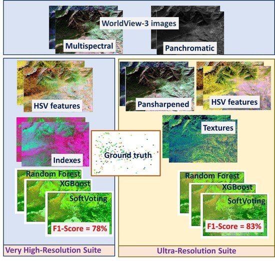
2. Materials and Methods
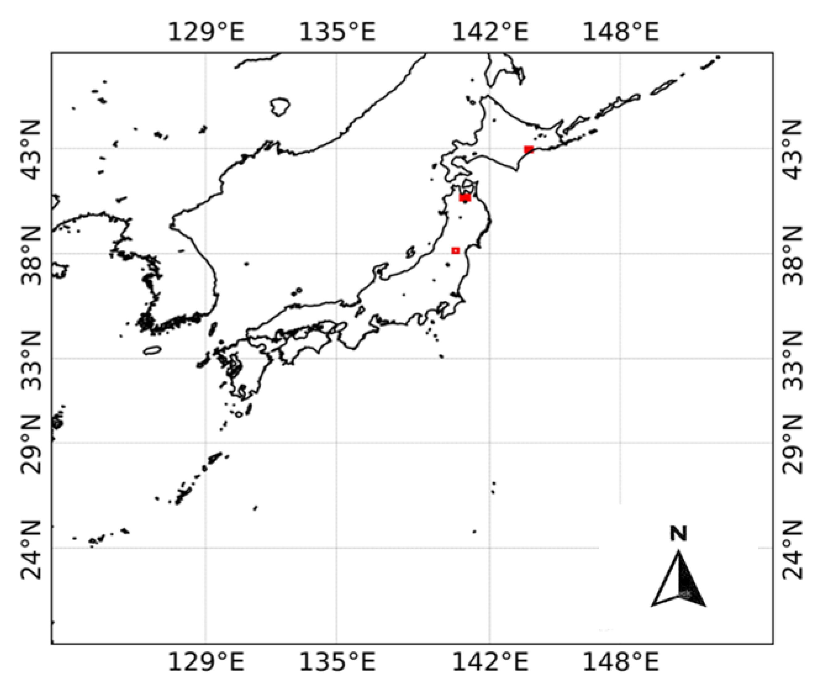
2.1. Study Area

This research was conducted at three study sites, Hakkoda, Zao, and Shiranuka, located in the Aomori, Miyagi, and Hokkaido prefectures in Japan, respectively. These sites represent mountainous cool temperate forest ecosystems. The location map of the study sites is shown in Figure 1.

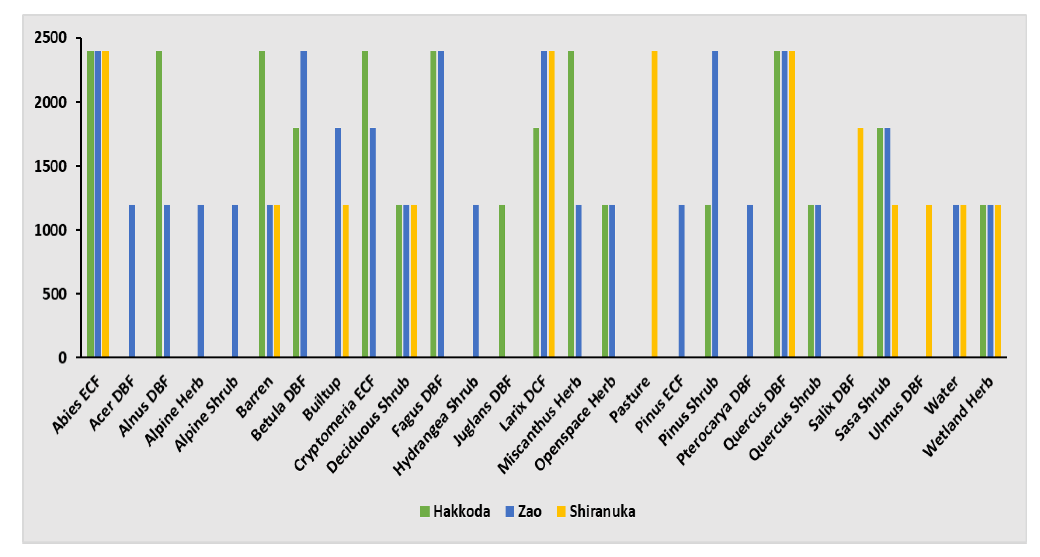
2.2. Collection of Ground Truth Data

This research utilized the ground truth data prepared in the previous study [54]. The ground truth data were prepared by field survey, accompanied with an existing vegetation survey map (1:25,000 scale), and visual interpretation of the time-lapse images available in Google Earth. The sample points (longitudes and latitudes) were prepared from homogenous areas belonging to each land cover and vegetation type concerned. In total, 1200–2400 sample points were prepared for each land cover and vegetation type for each site. The vegetation types were classified by adopting the genus–physiognomy–ecosystem system developed for satellite-based classification of plant communities in the previous study [55]. The ground truth data were prepared by considering unchanged areas between 2018–2020. However, since the study sites were usually devoid of human disturbances and landscape changes, the ground truth data could represent a few more nearby years. The distribution of the ground truth data size for each site is shown in Figure 2. The sample points were prepared by considering the proportional coverage of the land cover and vegetation types in each site. Therefore, vegetation types with large coverage, such as Abies ECF, Quercus DBF, and Fagus DBF, consisted of large sample sizes; whereas low-coverage vegetation types such as Acer DBF and Quercus Shrub received small sample sizes. This research dealt with the classification and mapping of 16 land cover and vegetation types in Hakkoda, 23 land cover and vegetation types in Zao, and 12 land cover and vegetation types in Shiranuka.

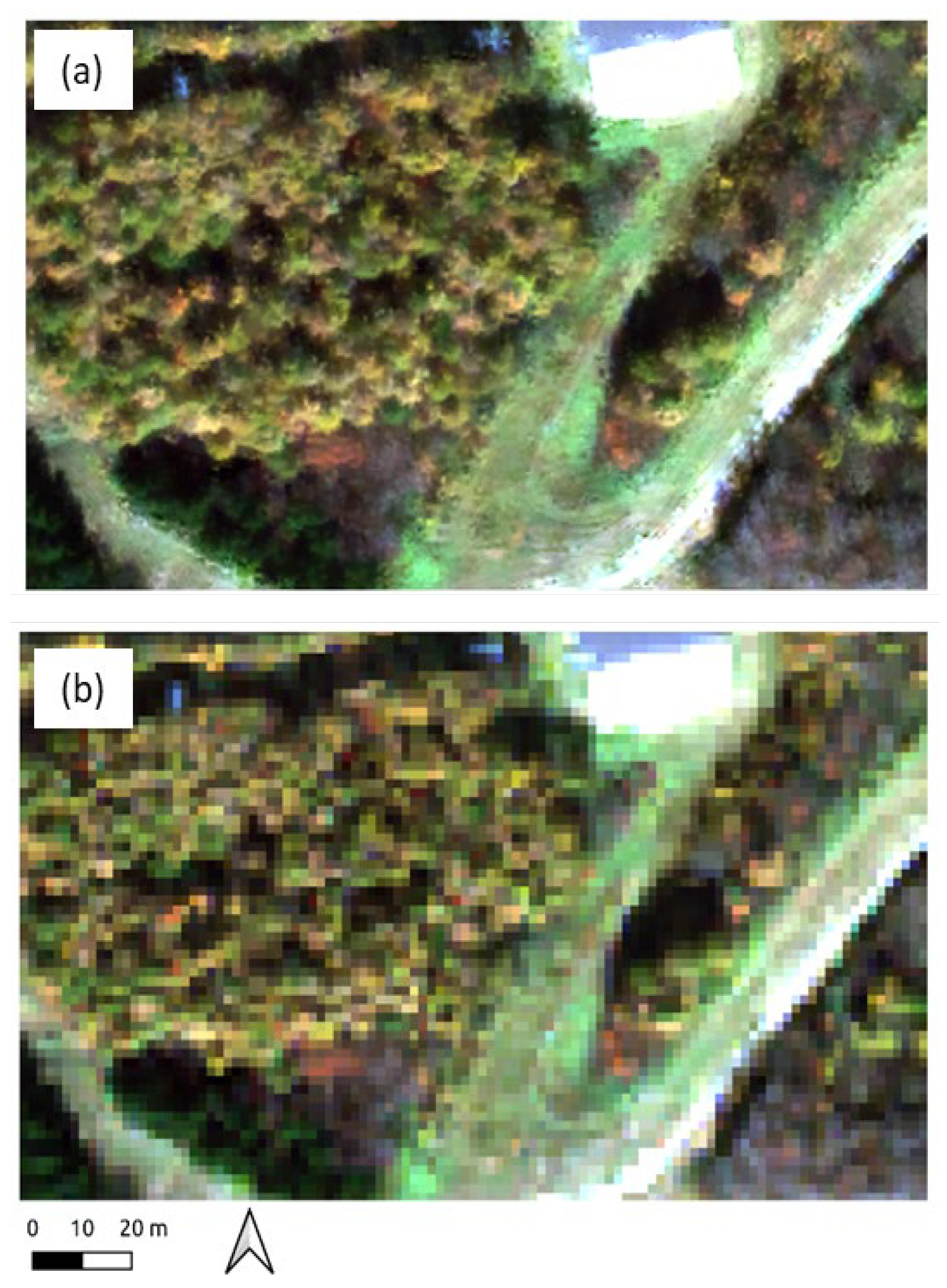
2.3. Processing of WorldView-3 Images

For each site, two cloud-free scenes taken by the WorldView-3 satellite were utilized in this research. The bi-seasonal WorldView-3 scenes acquired in the summer and autumn seasons for the Hakkoda (20 September 2019 and 10 June 2016), Zao (26 October 2017 and 8 September 2017), and Shiranuka (16 October 2020 and 1 June 2021) sites were utilized in the research. The summer and autumn seasons were chosen to capture phenological variations among the vegetation types because leaves are photosynthetically active during summer and deciduous shrubs and trees change color during autumn in the study sites located in cool temperate zones. Due to lack of cloud-free scenes available in the same year, the images were acquired from different years in two sites. However, the study sites were usually devoid of human disturbances and landscape changes and thus the acquired images were still appropriate.
WorldView-3 is a very high-resolution commercial imaging satellite which acquires 11-bit data in nine spectral bands (panchromatic, coastal, blue, green, yellow, red, red edge, near infrared 1, and near infrared 2), and additional 14-bit data in eight shortwave infrared bands. The nominal ground sample distances of the acquired images were 0.5 m for panchromatic and 2.0 m for multi-spectral images. Ortho-rectification of the WorldView-3 images was done using 30 m digital elevation model data [56] to remove geometric distortions [57,58] and topographic correction was done using a modified sun-canopy-sensor model [59,60]. The band-wise radiometric calibration factor and effective band width data were read from the metadata of the given WorldView-3 products and top-of-atmosphere radiance was calculated from the pixel-wise digital numbers. Then, the top-of-atmosphere reflectance was calculated accounting for the earth–sun distance, band-averaged solar spectral irradiance, and solar zenith angle [61].

2.4. Features Extraction

This research proposed two categories of feature extraction suite, a very high-resolution suite and an ultra-resolution suite for differentiation and mapping of land cover and vegetation types from a limited number of multi-spectral and panchromatic images. The features extraction flow of the ultra-resolution suite involves pan-sharpening of the multispectral image, color-transformation of the pan-sharpened image, and the generation of panchromatic textural features; whereas the very high-resolution features extraction suite involves the calculation of radiometric indices and color-transformation of the multi-spectral image.
For the very high-resolution suite, nine radiometric indices were calculated (Table 1) and combined with the multi-spectral image consisting of 8 bands (coastal, blue, green, yellow, red, red edge, near infrared 1, and near infrared 2), which yielded 17 spectral–radiometric features. In addition, the 8-band multispectral images were transformed into the Hue–Saturation–Value (HSV) color space. For this purpose, by taking 3 out of the 8 bands at a time, 120 permutations were calculated which yielded 336 sets of RGB images (1008 features). OpenCV (https://opencv.org, accessed on 15 April 2022)—Open Source Computer Vision Library—was used for the HSV transformations. It produced a large dimension of data in which some features exhibited multicollinearity. To cope with the complexity associated with the multicollinearity, 27 least-correlated features were extracted and combined with the 17 spectral–radiometric features prepared earlier.
For the ultra-resolution suite, pan-sharpening of the multi-spectral images (8 bands) was carried out with the panchromatic image using the local mean and variance matching method [71] to generate a pan-sharpened image (8 bands) at 0.5 m resolution. The 8-band pan-sharpened image was transformed into the Hue–Saturation–Value (HSV) color space and 27 least-correlated features were extracted from the pan-sharpened image in a manner similar to the HSV transformation of the very high-resolution suite. In addition, twenty-six Haralick’s textural images were generated from the panchromatic image using a sliding window of 3 × 3 pixels. To cope with the complexity associated with the multicollinearity, out of 18 textural features, 8 least-correlated features were extracted. Orfeo ToolBox (https://www.orfeo-toolbox.org, accessed on 15 April 2022)—an open-source C++ library for image processing—was used for pan-sharpening and the calculation of Haralick’s textures. A summary of the features extracted for the ultra-resolution and very high-resolution mapping suites is described in Table 2.

2.5. Machine Learning and Mapping

The pixel values corresponding to the ground truth data (geo-location points) were extracted from both the ultra-resolution and very high-resolution suites of images. Three machine learning classifiers, Random Forests (RF), eXtreme Gradient Boosting (XGBoost), and a predicted-probabilities-based fusion (SoftVoting) of the RF and XGBoost classifiers, were employed for the differentiation and mapping of land cover and vegetation types. Random Forests (RF) is an ensemble of decision trees, which are built by splitting the attributes of the data and averaging the output value of all trees [72]. The Gradient Boosting (GB) technique was designed to minimize the loss function of the model by adding weak learners [73]. XGBoost is one of the implementations of the Gradient Boosting technique designed for highly efficient and parallel machine learning capabilities [74]. The RF and XGboost classifiers have shown outstanding performance in classification of the satellite data [75,76,77,78,79,80]. Researchers have reported higher performance of the fusion of multiple classification results in land cover and vegetation mapping [81,82].
The ten-fold cross-validation method was utilized for quantitatively evaluating the performance of the ultra-resolution suite and the very high-resolution suite based on accuracy metrics, such as overall accuracy, kappa coefficient, F1-score, recall, and precision. After confirming the best-performed classifier and its parameters through the 10-fold cross-validation method, the best-performed model was built by training on 85% data for the prediction (mapping) of new data.

3. Results

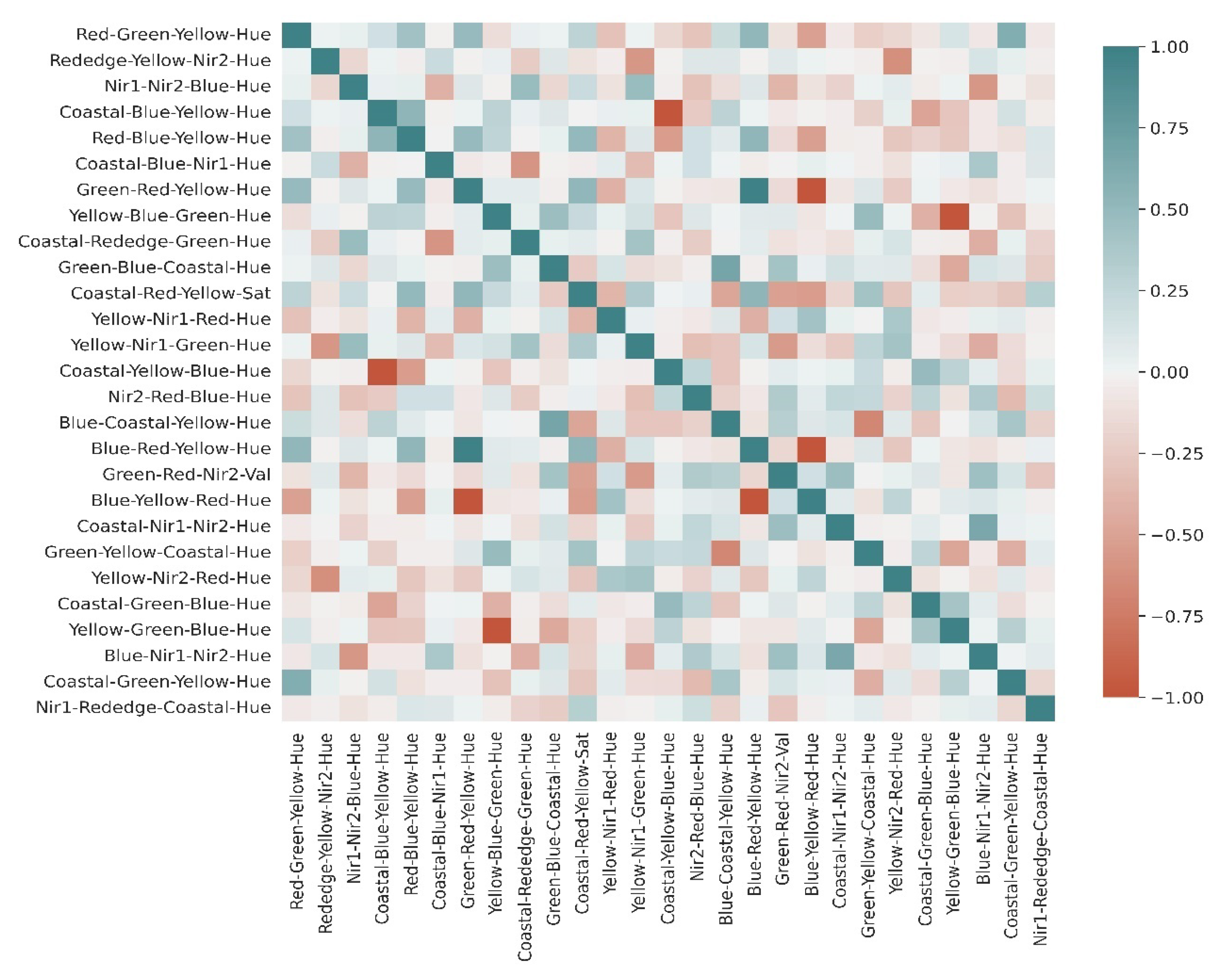
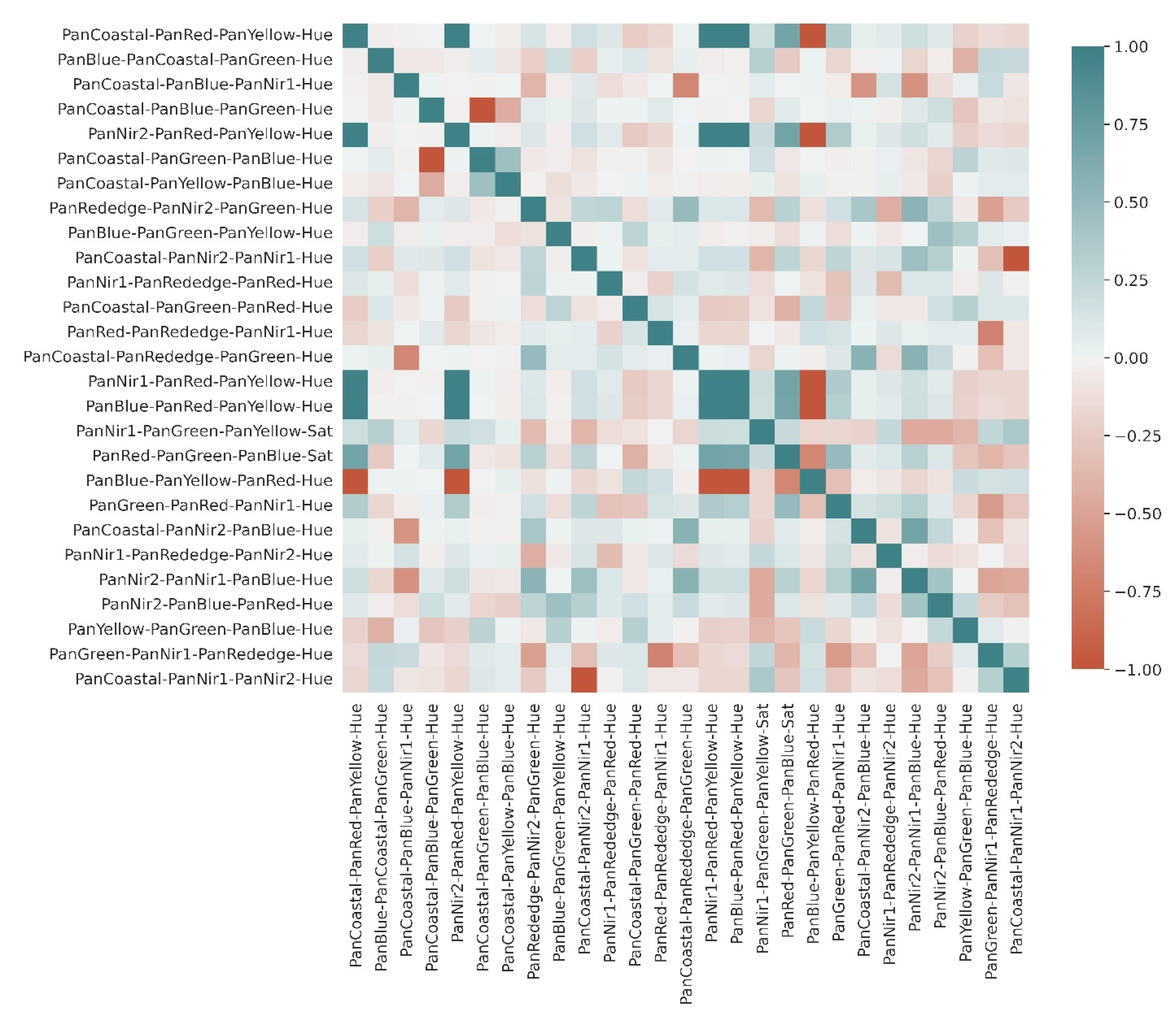
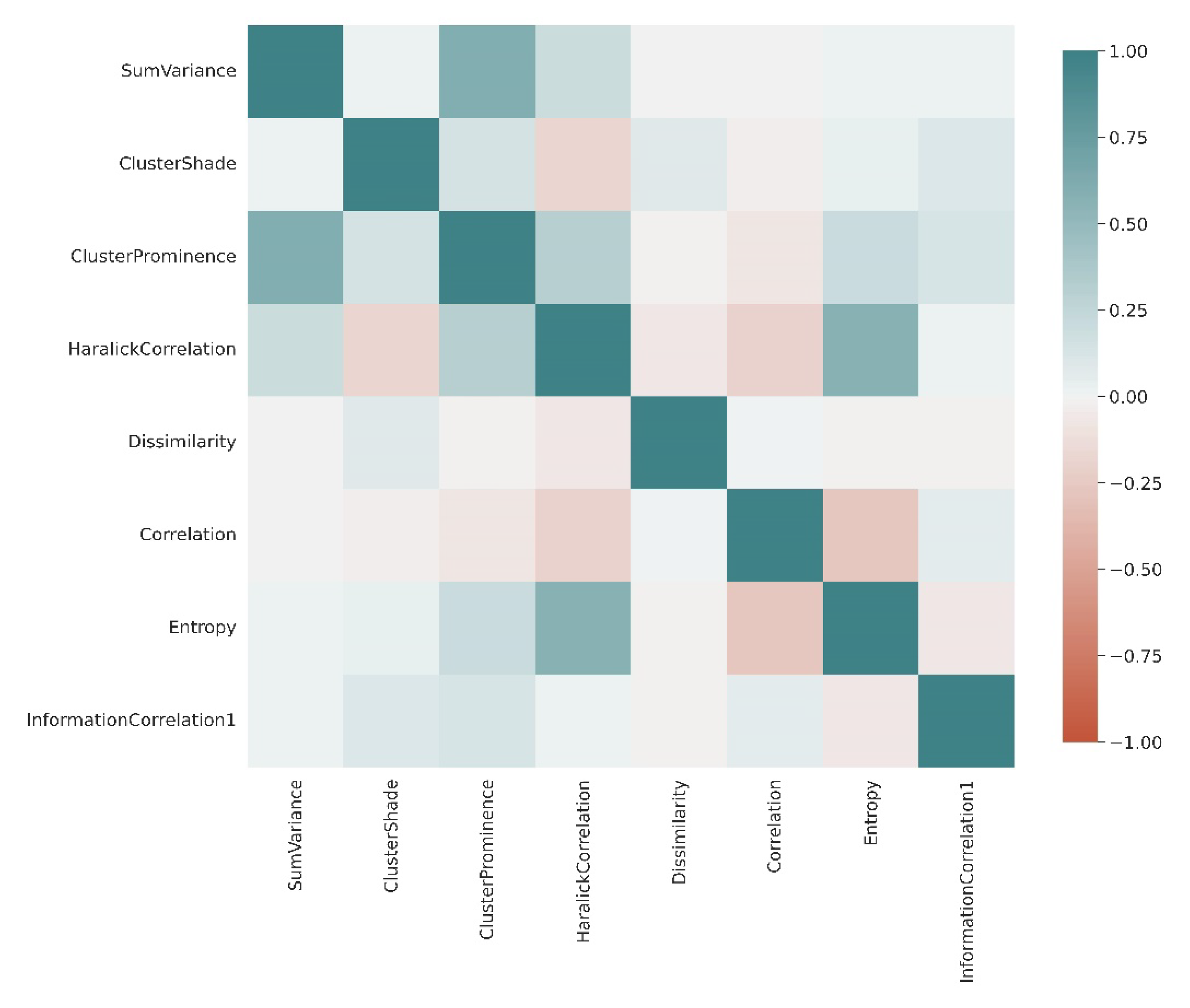
3.1. Extraction of Least-Correlated Features

The correlation matrix plot of the 27 least-correlated HSV features generated from the multispectral image is shown in Figure 3. None of the extracted features were correlated with more than a 0.7 Pearson correlation coefficient to each other. This is for the case of the single-date autumn images of the Shiranuka site. Likewise, for the pan-sharpened images, Figure 4 shows the 27 least-correlated HSV features generated in the case of the single-date autumn images of the Shiranuka site. In addition, the eight least-correlated textural features extracted based on the criteria of a Pearson correlation coefficient less than 0.7 is shown in Figure 5, in the case of the single-date autumn images of the Shiranuka site. The least-correlated features were extracted from the multispectral, pan-sharpened, and textural images for other seasons and other sites in a similar way.

3.2. Pan-Sharpened versus Multi-Spectral Images

An example demonstrating the superior capacity of a pan-sharpened image over a multispectral image for distinguishing the tree canopy is shown in Figure 6. In contrast to the multi-spectral image, the pan-sharpened image has captured the canopy details clearly and thus the pan-sharpened image is effective for distinguishing the plant communities.

3.3. Effect of Classifiers in the Case of Single-Date Autumn Images

The 10-fold cross-validation accuracies obtained from the two categories of features extraction suites (very high-resolution versus ultra-resolution) proposed in this research have been shown in Table 3 and Table 4. In all three sites (Hakkoda, Zao and Shiranuka) studied in this research, the SoftVoting classifier showed slightly better performance than the other two classifiers (XGBoost and Random Forests) without a substantial difference among the three classifiers (XGBoost, Random Forests, and SoftVoting).
The variation of the classification accuracy in terms of the F1-score with the classifier is summarized and shown in Figure 7. There was not a substantial difference among the three classifiers (XGBoost, Random Forests, and SoftVoting) employed for the classification of land cover and vegetation types using both categories of features extraction suite. In all sites, as described in Figure 7, the ultra-resolution suite showed superior performance over the very high-resolution suite using any machine learning classifier employed in the research. It should be noted that both suites utilized the same size of ground truth data.

3.4. Effect of Classifiers in the Case of Bi-Seasonal Images

The 10-fold cross-validation accuracies obtained from the two categories of features extraction suite (very high-resolution versus ultra-resolution) by using bi-seasonal images are shown in Table 5 and Table 6. Similar to the case of a single-date autumn image, the SoftVoting classifier showed slightly better performance than the other two classifiers (XGBoost and Random Forests) without substantial difference among the three classifiers in all sites.
The variation of the classification accuracy in terms of the F1-score with the classifier using bi-seasonal images is summarized and shown in Figure 8. Similar to the case of single-date autumn images, there was not a substantial difference among the three classifiers (XGBoost, Random Forests, and SoftVoting) employed for the classification of land cover and vegetation types using both categories of features extraction suite. However, in contrast to the case of single-date autumn images, performance of the RF was slightly lower than that of the XGBoost classifier. In all sites, as described in Figure 8, the ultra-resolution suite showed superior performance over the very high-resolution suite using any machine learning classifier employed in the research. It should be noted that both suites utilized the same size of ground truth data.

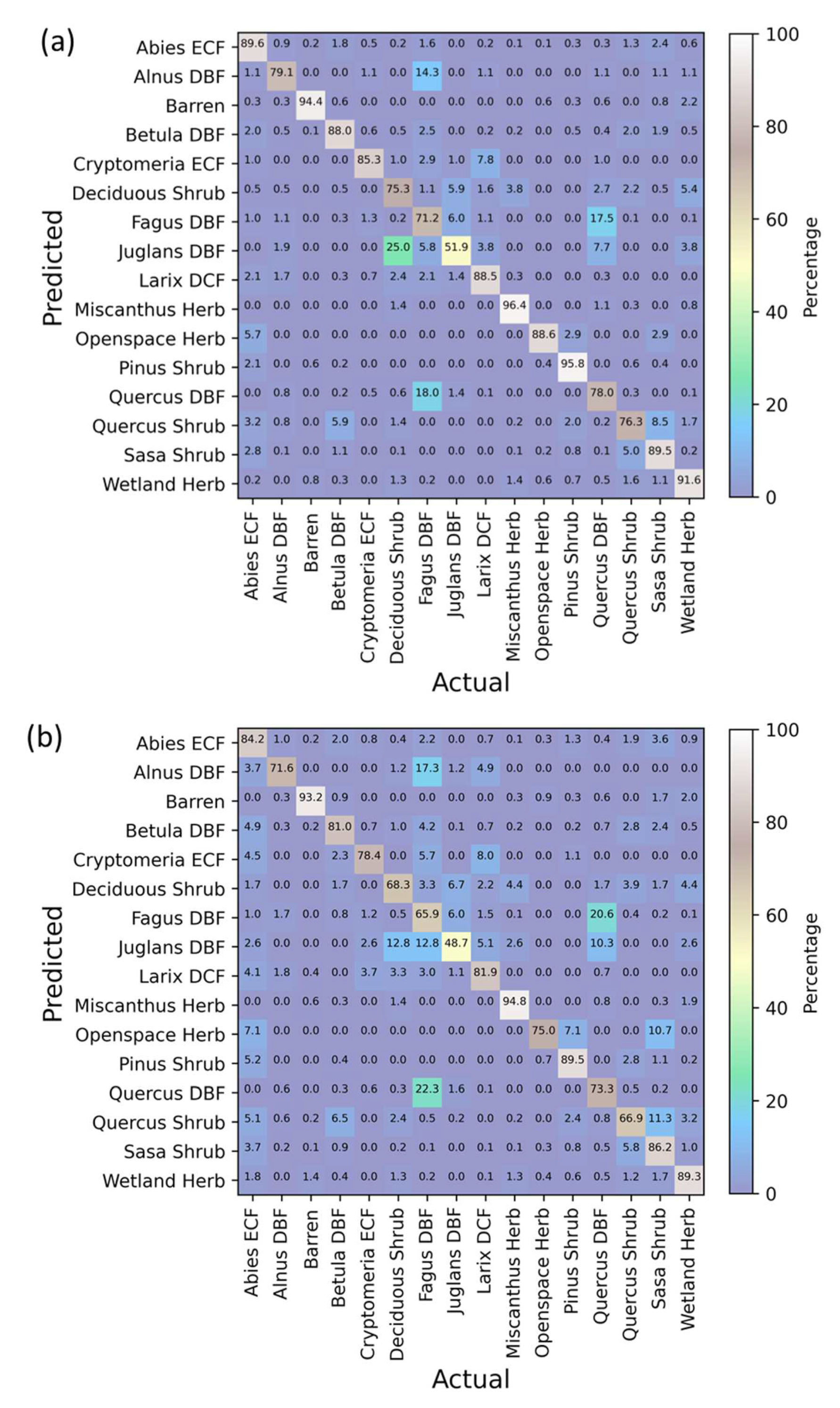
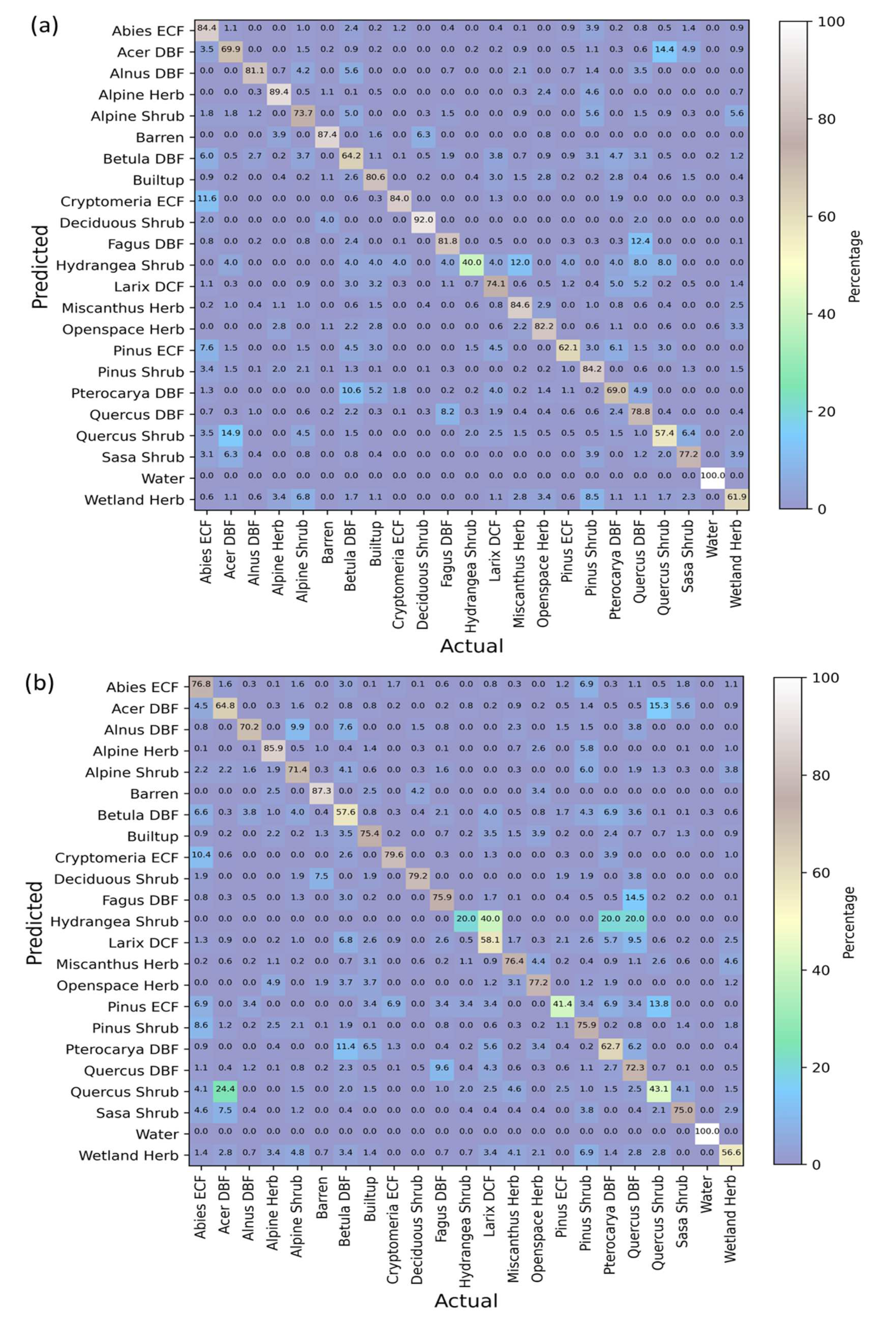
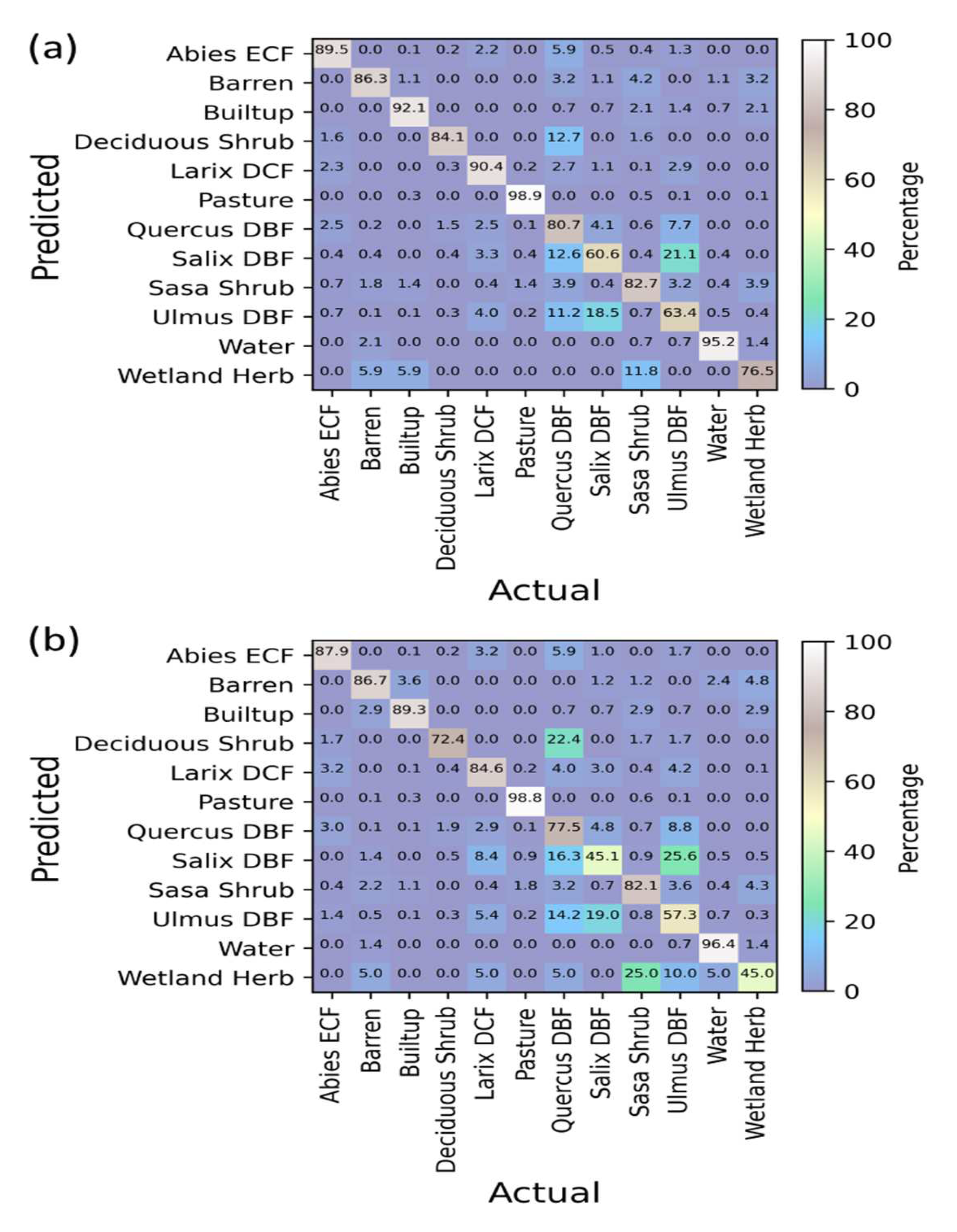
3.5. Confusion Matrices Using Bi-Seasonal Images

The confusion matrix figures calculated with the 10-fold cross-validation method using the SoftVoting classifier for the Hakkoda, Zao, and Shiranuka sites are shown in Figure 9, Figure 10 and Figure 11, respectively. Though most of the classes were discriminated satisfactorily, weak classification of some classes, for instance Juglans DBF, Fagus DBF, and Alnus DBF in site Hakkoda (Figure 9); Hydrangea Shrub and Pinus ECF in site Zao (Figure 10); and Salix DBF and Wetland Herb in site Shiranuka (Figure 11) was detected.

3.6. Class-Wise Changes

The changes in the class-wise accuracy by the addition of a summer image for each site are shown in Figure 12, Figure 13 and Figure 14 for the Hakkoda, Zao, and Shiranuka sites, respectively. The addition of summer images substantially increased the classification accuracy for most of the land cover and vegetation types in all sites studied. This improvement was substantial for both the ultra-resolution and very high-resolution mapping suites. The ultra-resolution suite using bi-seasonal images showed the highest performance in the differentiation of almost all land cover and vegetation types in all sites. This trend was followed by the very high-resolution suite using bi-seasonal images. The performance of both the ultra-resolution and very high-resolution suites using single-date autumn images was inferior to the performance gained by using bi-seasonal images with any feature extraction suite.

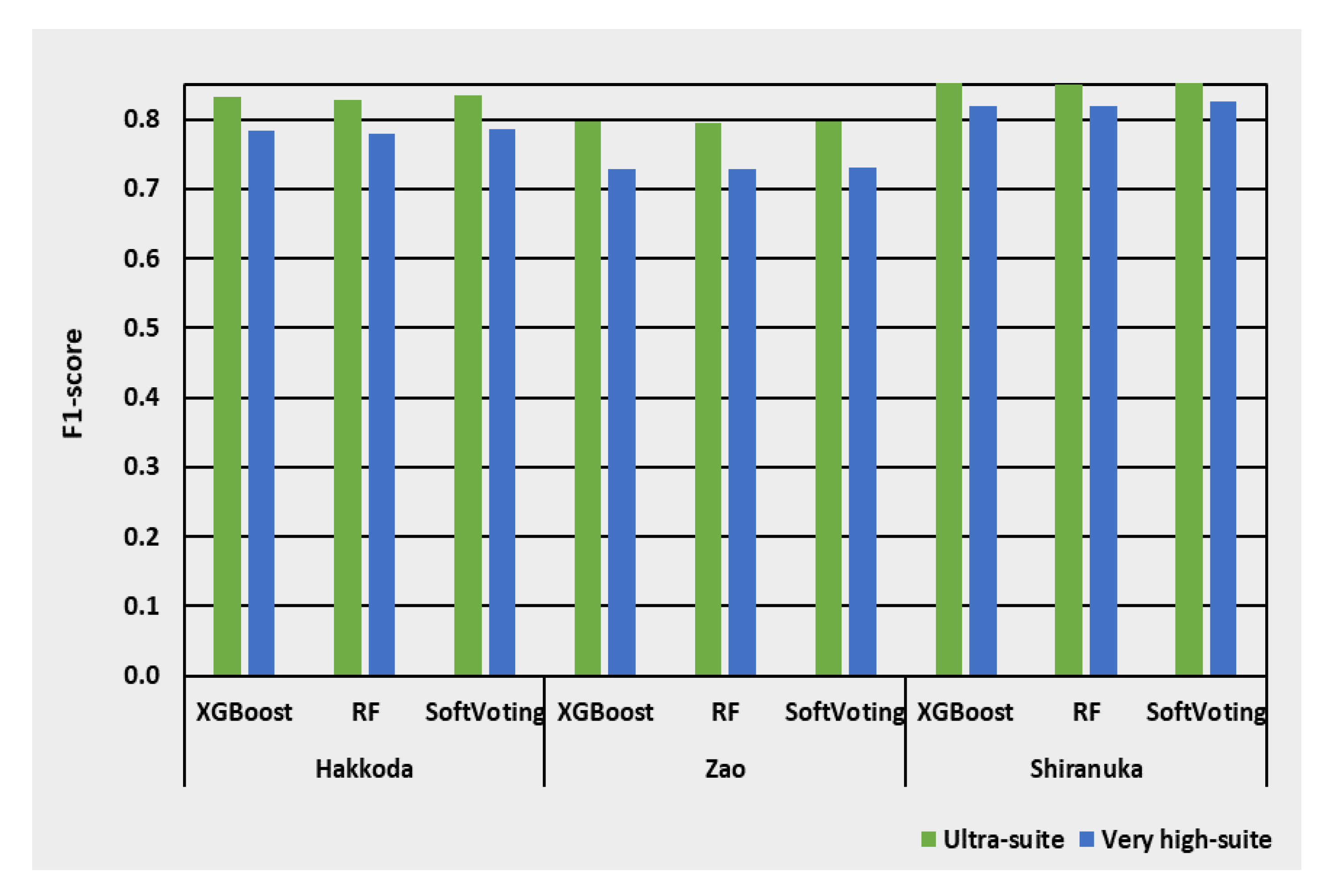
3.7. Performance Summary

The performance of the two categories of features extraction and mapping suites (ultra-resolution and very high-resolution suites) is summarized and shown in Figure 15. It is based on the 10-fold cross-validation accuracy (F1-score) using the SoftVoting classifier. For the case of single-date autumn images, the ultra-resolution suite provided 6.3% more accuracy (F1-score) than the very high-resolution suite in the Hakkoda site with 16 land cover and vegetation classes. In the Zao site with 23 classes, the ultra-resolution suite provided 6% more accuracy (F1-score) than the very high-resolution suite. For the classification of 12 classes in the Shiranuka site, the ultra-resolution suite provided 3.6% more accuracy (F1-score) than the very high-resolution suite. On average, the ultra-resolution suite provided 5.3% more accuracy (F1-score) than the very high-resolution suite across the three sites. A similar trend was obtained by using bi-seasonal images (summer and autumn). In the case of bi-seasonal images, the ultra-resolution suite provided 4.9% more accuracy in the Hakkoda site, 6.8% more accuracy in the Zao site, and 3% more accuracy in the Shiranuka site over the very high-resolution suite. On average, the ultra-resolution suite showed 4.9% higher performance than the very high-resolution suite using bi-seasonal images across three sites.
The addition of summer images with the previous autumn season images increased the classification accuracy substantially for both the ultra-resolution and very high-resolution suites in all sites. In the Hakkoda site, the gain by increasing the temporal images was 10.9% for the ultra-resolution suite and 12.3% for the very high-resolution suite. The Zao site gained 13.2% accuracy in the case of the ultra-resolution suite and 12.4% in the case of the very high-resolution suite. The gain by increasing the temporal images was 14.3% for the ultra-resolution suite and 14.9% for the very high-resolution suite in the Shiranuka site. On average, the ultra-resolution suite gained 12.8% accuracy; whereas 13.2% gain was achieved by the very high-resolution suite across the three sites. The very high-resolution suite gained slightly more accuracy than the ultra-resolution suite while increasing the temporal images.
However, it should be noted that the accuracy obtained from the ultra-resolution suite using single-date autumn images was not higher than the accuracy obtained from the very high-resolution suite using bi-seasonal images. Therefore, increasing the temporal images was found to be more crucial than the usage of ultra-resolution suites. Nevertheless, merely increasing the bi-temporal images was not found to be sufficient unless the ultra-resolution suite was applied.

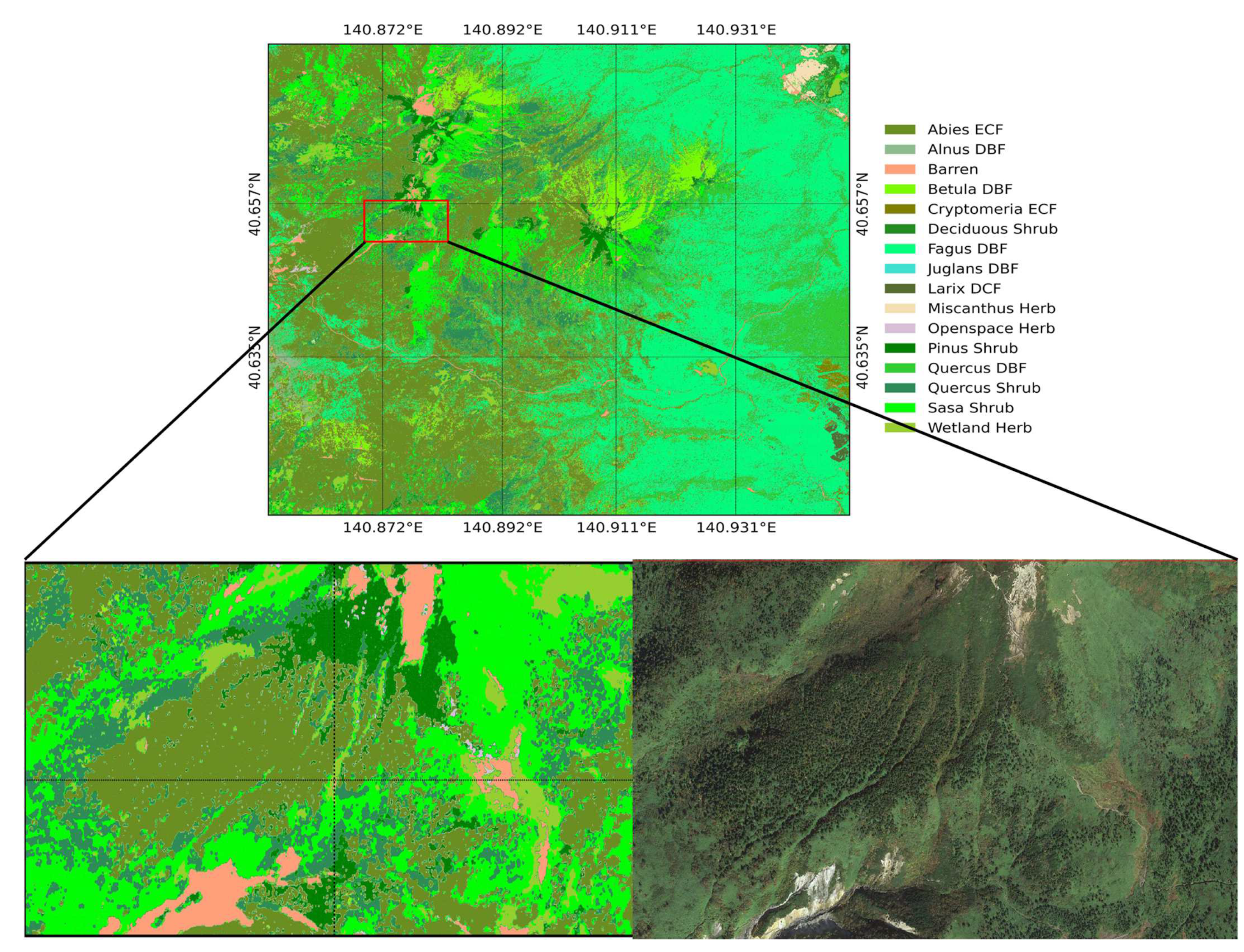
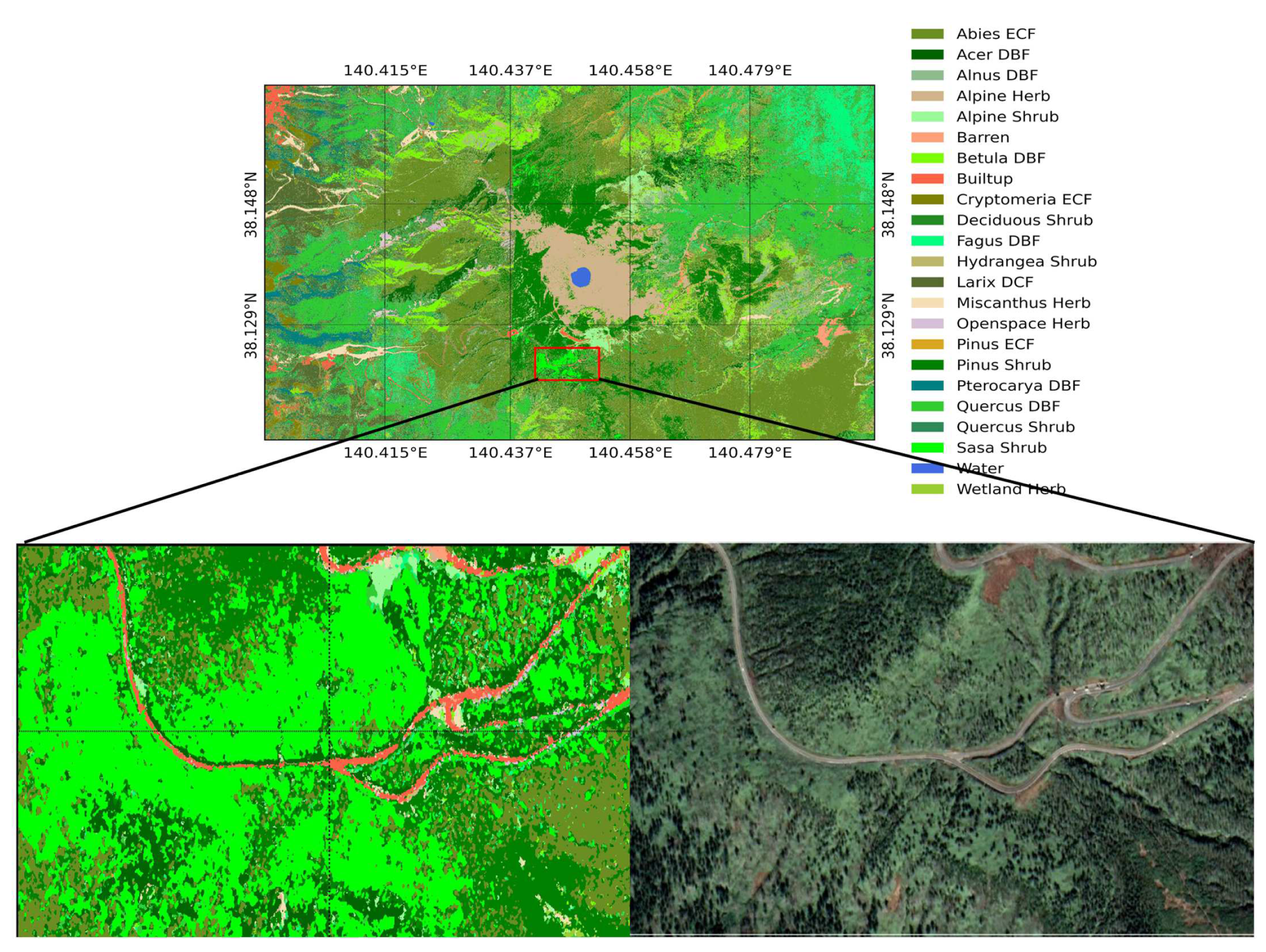
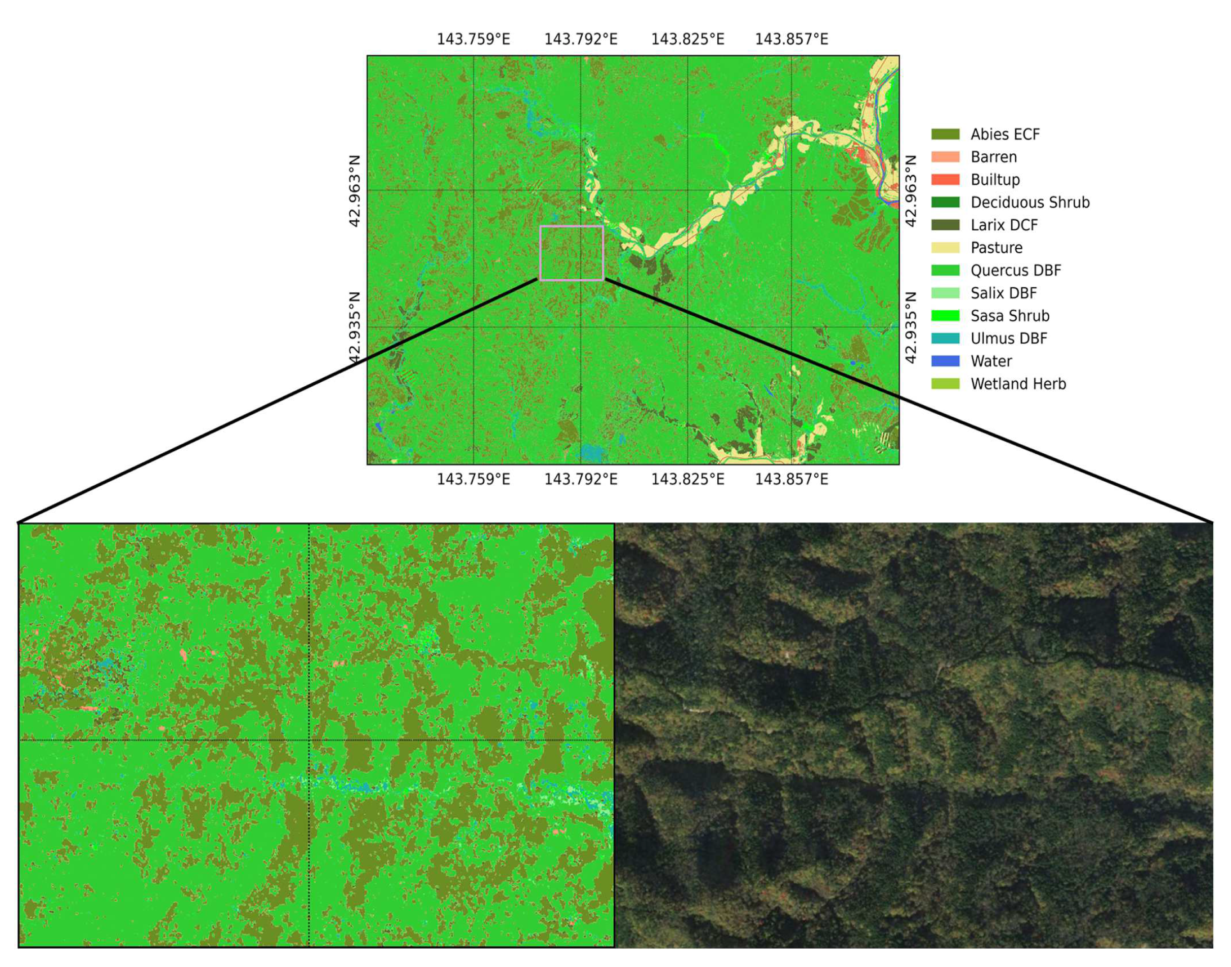
3.8. Ultra-Resolution Maps

Since the SoftVoting classifier showed slightly better performance than the Random Forests and XGBoost classifiers employed in the research, the SoftVoting classifier was chosen for the mapping of land cover and vegetation types. Furthermore, due to superior performance of the ultra-resolution suite over the very high-resolution suite using bi-seasonal images, the land cover and community-level vegetation maps were produced by utilizing the ultra-resolution suite using bi-temporal images. The ultra-resolution (0.5 m) land cover and community-level vegetation maps produced in this research are shown in Figure 16, Figure 17 and Figure 18 for the Hakkoda, Zao, and Shiranuka sites, respectively. These ultra-resolution maps show the detailed view and distribution of land cover and community-level vegetation types.
In Figure 16, the zoomed-in map (bottom left) shows the distribution of Abies ECF (olive color) among the Sasa Shrub (lime color) with some barren lands (pink red color). This distribution is well matched with the true-color composite image (bottom right). The dark green trees are Abies ECF in the true-color composite image whereas the light green areas are Sasa Shrub.
In Figure 17, the zoomed-in map (bottom left) shows the distribution of Abies ECF (olive color) and Pinus Shrub (dark green) among the Sasa Shrub (lime color) with built-up areas (red color). This distribution is well matched with the true-color composite image (bottom right). The dark green trees are Abies ECF and Pinus Shrub in the true-color composite image, whereas the light green shrubs are Sasa Shrub.
In Figure 18, the zoomed-in map (bottom left) shows the distribution of Abies ECF (olive color)) among the Quercus DBF (green color) with a few scattered barren pixels (pink red color). This distribution is well matched with the true-color composite image (bottom right). The dark green trees are Abies ECF in the true-color composite image, whereas the light green trees are Quercus DBF.

4. Discussion

In this research, we conducted ultra-resolution classification and mapping of land cover and vegetation types by employing machine learning techniques. Supervised classification of satellite images by employing machine learning classifiers such as Random Forests and XGBoost has been applied efficiently by previous studies for mapping of land cover and vegetation types [83,84]. The mapping suites presented in this research are built on the recent improvements of land cover and vegetation mapping through the utilization of machine learning and fusion of classification [85,86,87,88] and it indicates an enhanced performance by combining the probabilities of predictions from multiple classifiers. The ultra-resolution and very high-resolution suites proposed in this research should be effective and useful for land cover and vegetation mapping in other large regions of interest as well.
High-spatial-resolution images from earth-observing satellites have been effective for acquiring detailed information on land cover and vegetation types [89,90,91]. Previous studies have utilized high-spatial-resolution images for discriminating land cover and vegetation physiognomic types such as deciduous broad-leaved forests and evergreen broad-leaved forests [92,93,94,95,96]. Though some researchers have tried unsupervised segmentation and labeling methods such as k-means and hierarchical clustering techniques for land cover and vegetation classification and mapping [97,98], supervised classification of land cover and vegetation types by employing machine learning classifiers has been frequently utilized in recent studies [99,100].
Despite the free accessibility of high-resolution satellite images such as those from Sentinel-2 and Landsat 8, a number of ecological studies have utilized ultra-resolution and very high-resolution satellite images. Review of these studies indicates that ultra-resolution and very high-resolution satellite images have been adapted mainly for the detection and mapping of small patches of vegetation such as endangered plants and invasive species [101,102,103,104] or for the differentiation and mapping of mixed vegetation in a heterogeneous environment [105,106,107]. The vegetation mixedness is a matter of the spatial resolution of the imagery. The vegetation mixed in high-resolution imagery (e.g., 30 m resolution) can be unmixed in very high-resolution or ultra-resolution imagery. Therefore, very high-resolution or ultra-resolution imagery are very suitable for the mapping of mixed vegetation in a heterogeneous environment, as in this research.
The study led by Li et al. [108] for urban tree species mapping concluded that single-date WorldView-2 images did not produce satisfying classification results, with relatively low accuracy (44.7–82.5%), and found that usage of bi-temporal images could produce, on average, 10.7% higher accuracy. In a similar way, the addition of summer images to the previously used autumn-season images provided 12.8% higher accuracy for the ultra-resolution suite and 13.2% higher accuracy for the very high-resolution suite in this research across three cool temperate ecosystem sites. Wendelberger et al. [109] also explored bi-seasonal versus single-season WorldView-2 images to map three mangrove and four adjacent plant communities and found that bi-seasonal images were more effective than single-season to differentiate all communities of interest, in line with this research carried out in three mountainous ecosystems. Ferreira et al. [37] utilized WorldView-3 images acquired in the dry and wet seasons and emphasized the usage of seasonal images for tree species discrimination in semi-deciduous forests. The previous studies were also based on a limited number of temporal images, and thus improving the classification accuracy using limited temporal images, as carried out in this research, is an important contribution. The ultra-resolution suite involves pan-sharpening of the multispectral image, color-transformation of the pan-sharpened image, and the generation of panchromatic textural features. The advantages of pansharpened images and textural features have been reported by previous studies. Ibarrola-Ulzurrun et al. [110] described the effectiveness of pan-sharpening techniques to generate accurate vegetation maps in heterogenic and mixed ecosystems. Similarly, Castillejo-González [111] reported high performance of pansharpened QuickBird images for mapping of olive trees. Another study by Ferreira et al. [37] recommended the usage of texture features and pan-sharpening approaches for improved classification of tropical tree species from WorldView-3 satellite images. Therefore, the features extraction techniques implemented in this research are robust and trustworthy. In addition, the ultra-resolution suite expands these ideas by additional features retrieved from the color-transformation of the pan-sharpened images for distinguishing vegetation types at the community level such as Quercus DBF and Quercus Shrub.
On the other hand, the study led by Karlson et al. [112] compared wet season, dry season, and multi-seasonal WorldView-2 images for the classification of agroforestry tree species and found that the multi-seasonal dataset produced the most accurate classifications. Another study by Adamo et al. [113] has also focused on multi-seasonal images for the classification of grassland ecosystem types. Therefore, there is a possibility of increasing the accuracy further for the discrimination of complex vegetation types by the addition of more seasonal images in this research.

5. Conclusions

This research study proposed two categories of feature extraction suite, a very high-resolution suite and an ultra-resolution suite at 2 m and 0.5 m resolutions, respectively, and applied them for the differentiation and mapping of land cover and community-level vegetation types. In spite of a limited number of multi-spectral and panchromatic images available to the research, the ultra-resolution suite showed superior performance over the very high spatial resolution suite in all three sites studied. Achieving a 5.3% increase in the classification accuracy in terms of the F1-score using single-date images and a 4.9% increase in the classification accuracy using bi-seasonal images by the ultra-resolution suite are remarkable contributions. The ultra-resolution mapping suite based on pan-sharpened images and image textural properties has the capacity to capture plant communities cl to the individual canopy level. The image textural information incorporated by the ultra-resolution suite is not available for the very high-resolution suite. The ultra-resolution suite can be suitable for discovering small patches of rare and endangered species which would otherwise be difficult to detect solely from coarse-resolution images. The features extraction suites presented in this research can also be applied with more temporal images. Addition of more temporal images can be useful for retrieving detailed phenological information, and thus can increase the classification accuracy further. The ultra-resolution suite presented in this research is expected to meet the growing need for differentiating a wide variety of land cover and vegetation types, particularly at large regions of interest, irrespective of limited temporal images.

Funding

This research received no external funding.

Acknowledgments

The WorldView images utilized in this research were provided by JAXA-commissioned research in 2019–2021. Copyright of the WorldView data is inherited to Maxar (formally DigitalGlobe). Keitarou Hara is appreciated for logistic support to the research. The author is thankful to the anonymous reviewers and editors of the Journal.

Conflicts of Interest

The author declares no conflict of interest.

References

  1. Lauer, D.T.; Morain, S.A.; Salomonson, V.V. The Landsat Program: Its Origins, Evolution, and Impacts. Photogramm. Eng. Remote Sens. 1997, 63, 831–838. [Google Scholar]
  2. Woodcock, C.E.; Allen, R.; Anderson, M.; Belward, A.; Bindschadler, R.; Cohen, W.; Gao, F.; Goward, S.N.; Helder, D.; Helmer, E.; et al. Free Access to Landsat Imagery. Science 2008, 320, 1011. [Google Scholar] [CrossRef] [PubMed]
  3. Wulder, M.A.; Masek, J.G.; Cohen, W.B.; Loveland, T.R.; Woodcock, C.E. Opening the Archive: How Free Data Has Enabled the Science and Monitoring Promise of Landsat. Remote Sens. Environ. 2012, 122, 2–10. [Google Scholar] [CrossRef]
  4. Irons, J.R.; Dwyer, J.L.; Barsi, J.A. The next Landsat Satellite: The Landsat Data Continuity Mission. Remote Sens. Environ. 2012, 122, 11–21. [Google Scholar] [CrossRef] [Green Version]
  5. Zhu, Z.; Wulder, M.A.; Roy, D.P.; Woodcock, C.E.; Hansen, M.C.; Radeloff, V.C.; Healey, S.P.; Schaaf, C.; Hostert, P.; Strobl, P.; et al. Benefits of the Free and Open Landsat Data Policy. Remote Sens. Environ. 2019, 224, 382–385. [Google Scholar] [CrossRef]
  6. Drusch, M.; Del Bello, U.; Carlier, S.; Colin, O.; Fernandez, V.; Gascon, F.; Hoersch, B.; Isola, C.; Laberinti, P.; Martimort, P.; et al. Sentinel-2: ESA’s Optical High-Resolution Mission for GMES Operational Services. Remote Sens. Environ. 2012, 120, 25–36. [Google Scholar] [CrossRef]
  7. Li, J.; Roy, D. A Global Analysis of Sentinel-2A, Sentinel-2B and Landsat-8 Data Revisit Intervals and Implications for Terrestrial Monitoring. Remote Sens. 2017, 9, 902. [Google Scholar] [CrossRef] [Green Version]
  8. Anderson, N.T.; Marchisio, G.B. WorldView-2 and the Evolution of the DigitalGlobe Remote Sensing Satellite Constellation: Introductory Paper for the Special Session on WorldView-2. In Proceedings of the Algorithms and Technologies for Multispectral, Hyperspectral, and Ultraspectral Imagery XVIII, Baltimore, MD, USA, 23–27 April 2012; Shen, S.S., Lewis, P.E., Eds.; SPIE: Bellingham, WA, USA, 2012; pp. 166–180. [Google Scholar]
  9. Ustin, S.L.; Middleton, E.M. Current and Near-Term Advances in Earth Observation for Ecological Applications. Ecol. Process 2021, 10, 1. [Google Scholar] [CrossRef]
  10. Qin, R.; Liu, T. A Review of Landcover Classification with Very-High Resolution Remotely Sensed Optical Images—Analysis Unit, Model Scalability and Transferability. Remote Sens. 2022, 14, 646. [Google Scholar] [CrossRef]
  11. Ponzoni, F.J.; Galvão, L.S.; Epiphanio, J.C.N. Spatial Resolution Influence on the Identification of Land Cover Classes in the Amazon Environment. An. Acad. Bras. Ciênc. 2002, 74, 717–725. [Google Scholar] [CrossRef] [Green Version]
  12. Achard, F.; Eva, H.; Mayaux, P. Tropical Forest Mapping from Coarse Spatial Resolution Satellite Data: Production and Accuracy Assessment Issues. Int. J. Remote Sens. 2001, 22, 2741–2762. [Google Scholar] [CrossRef]
  13. Xu, K.; Zhang, Z.; Yu, W.; Zhao, P.; Yue, J.; Deng, Y.; Geng, J. How Spatial Resolution Affects Forest Phenology and Tree-Species Classification Based on Satellite and Up-Scaled Time-Series Images. Remote Sens. 2021, 13, 2716. [Google Scholar] [CrossRef]
  14. Liu, M.; Popescu, S.; Malambo, L. Effects of Spatial Resolution on Burned Forest Classification with ICESat-2 Photon Counting Data. Front. Remote Sens. 2021, 2, 666251. [Google Scholar] [CrossRef]
  15. Wulder, M.A.; Hall, R.J.; Coops, N.C.; Franklin, S.E. High Spatial Resolution Remotely Sensed Data for Ecosystem Characterization. BioScience 2004, 54, 511. [Google Scholar] [CrossRef] [Green Version]
  16. Wickham, J.; Riitters, K.H. Influence of High-Resolution Data on the Assessment of Forest Fragmentation. Landsc. Ecol. 2019, 34, 2169–2182. [Google Scholar] [CrossRef] [Green Version]
  17. Durgun, Y.Ö.; Gobin, A.; Duveiller, G.; Tychon, B. A Study on Trade-Offs between Spatial Resolution and Temporal Sampling Density for Wheat Yield Estimation Using Both Thermal and Calendar Time. Int. J. Appl. Earth Obs. Geoinf. 2020, 86, 101988. [Google Scholar] [CrossRef]
  18. Monasterio, M.; Sarmiento, G. Phenological Strategies of Plant Species in the Tropical Savanna and the Semi-Deciduous Forest of the Venezuelan Llanos. J. Biogeogr. 1976, 3, 325. [Google Scholar] [CrossRef] [Green Version]
  19. de L. Brooke, M.; Jones, P.J.; Vickery, J.A.; Waldren, S. Seasonal Patterns of Leaf Growth and Loss, Flowering and Fruiting on a Subtropical Central Pacific Island. Biotropica 1996, 28, 164. [Google Scholar] [CrossRef]
  20. Xue, J.; Su, B. Significant Remote Sensing Vegetation Indices: A Review of Developments and Applications. J. Sens. 2017, 2017, 1–17. [Google Scholar] [CrossRef] [Green Version]
  21. Lee, J.-H.; Chang, B.-H.; Kim, S.-D. Comparison of Colour Transformations for Image Segmentation. Electron. Lett. 1994, 30, 1660–1661. [Google Scholar] [CrossRef]
  22. Reed, T.R.; Dubuf, J.M.H. A Review of Recent Texture Segmentation and Feature Extraction Techniques. CVGIP Image Underst. 1993, 57, 359–372. [Google Scholar] [CrossRef]
  23. Humeau-Heurtier, A. Texture Feature Extraction Methods: A Survey. IEEE Access 2019, 7, 8975–9000. [Google Scholar] [CrossRef]
  24. Smith, A.R. Color Gamut Transform Pairs. In Proceedings of the 5th Annual Conference on Computer Graphics and Interactive techniques—SIGGRAPH ’78, Atlanta, GA, USA, 23–25 August 1978; ACM Press: New York, NY, USA, 1978; pp. 12–19. [Google Scholar]
  25. Hamuda, E.; Mc Ginley, B.; Glavin, M.; Jones, E. Automatic Crop Detection under Field Conditions Using the HSV Colour Space and Morphological Operations. Comput. Electron. Agric. 2017, 133, 97–107. [Google Scholar] [CrossRef]
  26. Chang, C.-L.; Lin, K.-M. Smart Agricultural Machine with a Computer Vision-Based Weeding and Variable-Rate Irrigation Scheme. Robotics 2018, 7, 38. [Google Scholar] [CrossRef] [Green Version]
  27. Wang, D.; Fang, S.; Yang, Z.; Wang, L.; Tang, W.; Li, Y.; Tong, C. A Regional Mapping Method for Oilseed Rape Based on HSV Transformation and Spectral Features. Int. J. Geo-Inf. 2018, 7, 224. [Google Scholar] [CrossRef] [Green Version]
  28. Iovan, C.; Boldo, D.; Cord, M. Detection, Characterization, and Modeling Vegetation in Urban Areas from High-Resolution Aerial Imagery. IEEE J. Sel. Top. Appl. Earth Obs. Remote Sens. 2008, 1, 206–213. [Google Scholar] [CrossRef]
  29. Liu, H.; An, H. Urban Greening Tree Species Classification Based on HSV Colour Space of WorldView-2. J. Indian Soc. Remote Sens. 2019, 47, 1959–1967. [Google Scholar] [CrossRef]
  30. Haralick, R.M.; Shanmugam, K.; Dinstein, I. Textural Features for Image Classification. IEEE Trans. Syst. Man Cybern. 1973, SMC-3, 610–621. [Google Scholar] [CrossRef] [Green Version]
  31. Mishra, V.N.; Prasad, R.; Rai, P.K.; Vishwakarma, A.K.; Arora, A. Performance Evaluation of Textural Features in Improving Land Use/Land Cover Classification Accuracy of Heterogeneous Landscape Using Multi-Sensor Remote Sensing Data. Earth Sci. Inform. 2019, 12, 71–86. [Google Scholar] [CrossRef]
  32. Farwell, L.S.; Gudex-Cross, D.; Anise, I.E.; Bosch, M.J.; Olah, A.M.; Radeloff, V.C.; Razenkova, E.; Rogova, N.; Silveira, E.M.O.; Smith, M.M.; et al. Satellite Image Texture Captures Vegetation Heterogeneity and Explains Patterns of Bird Richness. Remote Sens. Environ. 2021, 253, 112175. [Google Scholar] [CrossRef]
  33. Guo, W.; Rees, G.; Hofgaard, A. Delineation of the Forest-Tundra Ecotone Using Texture-Based Classification of Satellite Imagery. Int. J. Remote Sens. 2020, 41, 6384–6408. [Google Scholar] [CrossRef]
  34. Ireland, A.W.; Smith, F.G.F.; Jaffe, B.D.; Palandro, D.A.; Mercer, S.M.; Liu, L.; Renton, J. Field Experiment Demonstrates the Potential Utility of Satellite-Derived Reflectance Indices for Monitoring Regeneration of Boreal Forest Communities. Trees For. People 2021, 6, 100145. [Google Scholar] [CrossRef]
  35. Wang, M.; Fei, X.; Zhang, Y.; Chen, Z.; Wang, X.; Tsou, J.Y.; Liu, D.; Lu, X. Assessing Texture Features to Classify Coastal Wetland Vegetation from High Spatial Resolution Imagery Using Completed Local Binary Patterns (CLBP). Remote Sens. 2018, 10, 778. [Google Scholar] [CrossRef] [Green Version]
  36. Zhang, X.; Cui, J.; Wang, W.; Lin, C. A Study for Texture Feature Extraction of High-Resolution Satellite Images Based on a Direction Measure and Gray Level Co-Occurrence Matrix Fusion Algorithm. Sensors 2017, 17, 1474. [Google Scholar] [CrossRef] [Green Version]
  37. Ferreira, M.P.; Wagner, F.H.; Aragão, L.E.O.C.; Shimabukuro, Y.E.; de Souza Filho, C.R. Tree Species Classification in Tropical Forests Using Visible to Shortwave Infrared WorldView-3 Images and Texture Analysis. ISPRS J. Photogramm. Remote Sens. 2019, 149, 119–131. [Google Scholar] [CrossRef]
  38. Tamondong, A.M.; Blanco, A.C.; Fortes, M.D.; Nadaoka, K. Mapping of Seagrass and Other Benthic Habitats in Bolinao, Pangasinan Using Worldview-2 Satellite Image. In Proceedings of the 2013 IEEE International Geoscience and Remote Sensing Symposium—IGARSS, Melbourne, Australia, 21–26 July 2013; IEEE: Piscataway, NJ, USA, 2013; pp. 1579–1582. [Google Scholar]
  39. Carle, M.V.; Wang, L.; Sasser, C.E. Mapping Freshwater Marsh Species Distributions Using WorldView-2 High-Resolution Multispectral Satellite Imagery. Int. J. Remote Sens. 2014, 35, 4698–4716. [Google Scholar] [CrossRef]
  40. Collin, A.; Lambert, N.; Etienne, S. Satellite-Based Salt Marsh Elevation, Vegetation Height, and Species Composition Mapping Using the Superspectral WorldView-3 Imagery. Int. J. Remote Sens. 2018, 39, 5619–5637. [Google Scholar] [CrossRef]
  41. Immitzer, M.; Atzberger, C.; Koukal, T. Tree Species Classification with Random Forest Using Very High Spatial Resolution 8-Band WorldView-2 Satellite Data. Remote Sens. 2012, 4, 2661–2693. [Google Scholar] [CrossRef] [Green Version]
  42. Pu, R.; Landry, S. A Comparative Analysis of High Spatial Resolution IKONOS and WorldView-2 Imagery for Mapping Urban Tree Species. Remote Sens. Environ. 2012, 124, 516–533. [Google Scholar] [CrossRef]
  43. Waser, L.; Küchler, M.; Jütte, K.; Stampfer, T. Evaluating the Potential of WorldView-2 Data to Classify Tree Species and Different Levels of Ash Mortality. Remote Sens. 2014, 6, 4515–4545. [Google Scholar] [CrossRef] [Green Version]
  44. Jombo, S.; Adam, E.; Odindi, J. Classification of Tree Species in a Heterogeneous Urban Environment Using Object-Based Ensemble Analysis and World View-2 Satellite Imagery. Appl. Geomat. 2021, 13, 373–387. [Google Scholar] [CrossRef]
  45. Ngubane, Z.; Odindi, J.; Mutanga, O.; Slotow, R. Assessment of the Contribution of WorldView-2 Strategically Positioned Bands in Bracken Fern (Pteridium aquilinum (L.) Kuhn) Mapping. S. Afr. J. Geomat. 2014, 3, 210. [Google Scholar] [CrossRef] [Green Version]
  46. Adam, E.; Mureriwa, N.; Newete, S. Mapping Prosopis Glandulosa (Mesquite) in the Semi-Arid Environment of South Africa Using High-Resolution WorldView-2 Imagery and Machine Learning Classifiers. J. Arid Environ. 2017, 145, 43–51. [Google Scholar] [CrossRef]
  47. Mureriwa, N.F.; Adam, E.; Adelabu, S. Cost Effective Approach for Mapping Prosopis Invasion in Arid South Africa Using SPOT-6 Imagery and Two Machine Learning Classifiers. In Proceedings of the IGARSS 2019—2019 IEEE International Geoscience and Remote Sensing Symposium, Yokohama, Japan, 28 July–2 August 2019; IEEE: Piscataway, NJ, USA, 2019; pp. 3724–3727. [Google Scholar]
  48. Schulze-Brüninghoff, D.; Wachendorf, M.; Astor, T. Potentials and Limitations of WorldView-3 Data for the Detection of Invasive Lupinus Polyphyllus Lindl. in Semi-Natural Grasslands. Remote Sens. 2021, 13, 4333. [Google Scholar] [CrossRef]
  49. Novack, T.; Esch, T.; Kux, H.; Stilla, U. Machine Learning Comparison between WorldView-2 and QuickBird-2-Simulated Imagery Regarding Object-Based Urban Land Cover Classification. Remote Sens. 2011, 3, 2263–2282. [Google Scholar] [CrossRef] [Green Version]
  50. Heumann, B.W. An Object-Based Classification of Mangroves Using a Hybrid Decision Tree—Support Vector Machine Approach. Remote Sens. 2011, 3, 2440–2460. [Google Scholar] [CrossRef] [Green Version]
  51. Kavzoglu, T.; Colkesen, I.; Yomralioglu, T. Object-Based Classification with Rotation Forest Ensemble Learning Algorithm Using Very-High-Resolution WorldView-2 Image. Remote Sens. Lett. 2015, 6, 834–843. [Google Scholar] [CrossRef]
  52. Chuang, Y.-C.; Shiu, Y.-S. A Comparative Analysis of Machine Learning with WorldView-2 Pan-Sharpened Imagery for Tea Crop Mapping. Sensors 2016, 16, 594. [Google Scholar] [CrossRef] [Green Version]
  53. Jackson, C.M.; Adam, E. Machine Learning Classification of Endangered Tree Species in a Tropical Submontane Forest Using WorldView-2 Multispectral Satellite Imagery and Imbalanced Dataset. Remote Sens. 2021, 13, 4970. [Google Scholar] [CrossRef]
  54. Sharma, R.C.; Hirayama, H.; Yasuda, M.; Asai, M.; Hara, K. Classification and Mapping of Plant Communities Using Multi-Temporal and Multi-Spectral Satellite Images. J. Geogr. Geol. 2022, 14, 43. [Google Scholar] [CrossRef]
  55. Sharma, R.C. Genus-Physiognomy-Ecosystem (GPE) System for Satellite-Based Classification of Plant Communities. Ecologies 2021, 2, 203–213. [Google Scholar] [CrossRef]
  56. Farr, T.G.; Rosen, P.A.; Caro, E.; Crippen, R.; Duren, R.; Hensley, S.; Kobrick, M.; Paller, M.; Rodriguez, E.; Roth, L.; et al. The Shuttle Radar Topography Mission. Rev. Geophys. 2007, 45, RG2004. [Google Scholar] [CrossRef] [Green Version]
  57. Aguilar, M.A.; del Saldaña, M.M.; Aguilar, F.J. Assessing Geometric Accuracy of the Orthorectification Process from GeoEye-1 and WorldView-2 Panchromatic Images. Int. J. Appl. Earth Obs. Geoinf. 2013, 21, 427–435. [Google Scholar] [CrossRef]
  58. Belfiore, O.; Parente, C. Comparison of Different Algorithms to Orthorectify WorldView-2 Satellite Imagery. Algorithms 2016, 9, 67. [Google Scholar] [CrossRef]
  59. Soenen, S.A.; Peddle, D.R.; Coburn, C.A. SCS+C: A Modified Sun-Canopy-Sensor Topographic Correction in Forested Terrain. IEEE Trans. Geosci. Remote Sens. 2005, 43, 2148–2159. [Google Scholar] [CrossRef]
  60. Richter, R.; Kellenberger, T.; Kaufmann, H. Comparison of Topographic Correction Methods. Remote Sens. 2009, 1, 184–196. [Google Scholar] [CrossRef] [Green Version]
  61. Updike, T.; Comp, C. Radiometric Use of WorldView-2 Imagery; Technical Note; DigitalGlobe: Longmont, CO, USA, 2010; pp. 1–17. [Google Scholar]
  62. Rouse, J.W.; Haas, R.H.; Schell, J.A.; Deering, D.W. Monitoring Vegetation Systems in the Great Plains with ERTS. NASA Spec. Publ. 1974, 351, 309. [Google Scholar]
  63. Falkowski, M.J.; Gessler, P.E.; Morgan, P.; Hudak, A.T.; Smith, A.M.S. Characterizing and Mapping Forest Fire Fuels Using ASTER Imagery and Gradient Modeling. For. Ecol. Manag. 2005, 217, 129–146. [Google Scholar] [CrossRef] [Green Version]
  64. Huete, A.R. A Soil-Adjusted Vegetation Index (SAVI). Remote Sens. Environ. 1988, 25, 295–309. [Google Scholar] [CrossRef]
  65. Qi, J.; Chehbouni, A.; Huete, A.R.; Kerr, Y.H.; Sorooshian, S. A Modified Soil Adjusted Vegetation Index. Remote Sens. Environ. 1994, 48, 119–126. [Google Scholar] [CrossRef]
  66. Kaufman, Y.J.; Tanre, D. Atmospherically Resistant Vegetation Index (ARVI) for EOS-MODIS. IEEE Trans. Geosci. Remote Sens. 1992, 30, 261–270. [Google Scholar] [CrossRef]
  67. Daughtry, C. Estimating Corn Leaf Chlorophyll Concentration from Leaf and Canopy Reflectance. Remote Sens. Environ. 2000, 74, 229–239. [Google Scholar] [CrossRef]
  68. Wolf, A.F. Using WorldView-2 Vis-NIR Multispectral Imagery to Support Land Mapping and Feature Extraction Using Normalized Difference Index Ratios. In Proceedings of the Algorithms and Technologies for Multispectral, Hyperspectral, and Ultraspectral Imagery XVIII, Baltimore, MD, USA, 23–27 April 2012; Shen, S.S., Lewis, P.E., Eds.; SPIE: Bellingham, WA, USA, 2012; pp. 188–195. [Google Scholar]
  69. Penuelas, J.; Frederic, B.; Filella, I. Semi-Empirical Indices to Assess Carotenoids/Chlorophyll-a Ratio from Leaf Spectral Reflectance. Photosynthetica 1995, 31, 221–230. [Google Scholar]
  70. Huete, A.; Didan, K.; Miura, T.; Rodriguez, E.P.; Gao, X.; Ferreira, L.G. Overview of the Radiometric and Biophysical Performance of the MODIS Vegetation Indices. Remote Sens. Environ. 2002, 83, 195–213. [Google Scholar] [CrossRef]
  71. Mhangara, P.; Mapurisa, W.; Mudau, N. Comparison of Image Fusion Techniques Using Satellite Pour l’Observation de La Terre (SPOT) 6 Satellite Imagery. Appl. Sci. 2020, 10, 1881. [Google Scholar] [CrossRef] [Green Version]
  72. Breiman, L. Random Forests. Mach. Learn. 2001, 45, 5–32. [Google Scholar] [CrossRef] [Green Version]
  73. Friedman, J.H. Greedy Function Approximation: A Gradient Boosting Machine. Ann. Stat. 2001, 29, 1189–1232. [Google Scholar] [CrossRef]
  74. Chen, T.; Guestrin, C. XGBoost: A Scalable Tree Boosting System. In Proceedings of the 22nd ACM SIGKDD International Conference on Knowledge Discovery and Data Mining, San Francisco, CA, USA, 13–17 August 2016; ACM: New York, NY, USA, 2016; pp. 785–794. [Google Scholar]
  75. Mitchell, R.; Frank, E. Accelerating the XGBoost Algorithm Using GPU Computing. PeerJ Comput. Sci. 2017, 3, e127. [Google Scholar] [CrossRef]
  76. Bhagwat, R.U.; Uma Shankar, B. A Novel Multilabel Classification of Remote Sensing Images Using XGBoost. In Proceedings of the 2019 IEEE 5th International Conference for Convergence in Technology (I2CT), Bombay, India, 29–31 March 2019; IEEE: Bombay, India, 2019; pp. 1–5. [Google Scholar]
  77. Zhang, H.; Eziz, A.; Xiao, J.; Tao, S.; Wang, S.; Tang, Z.; Zhu, J.; Fang, J. High-Resolution Vegetation Mapping Using EXtreme Gradient Boosting Based on Extensive Features. Remote Sens. 2019, 11, 1505. [Google Scholar] [CrossRef] [Green Version]
  78. Muthoka, J.M.; Salakpi, E.E.; Ouko, E.; Yi, Z.-F.; Antonarakis, A.S.; Rowhani, P. Mapping Opuntia Stricta in the Arid and Semi-Arid Environment of Kenya Using Sentinel-2 Imagery and Ensemble Machine Learning Classifiers. Remote Sens. 2021, 13, 1494. [Google Scholar] [CrossRef]
  79. Zhang, T.; Su, J.; Xu, Z.; Luo, Y.; Li, J. Sentinel-2 Satellite Imagery for Urban Land Cover Classification by Optimized Random Forest Classifier. Appl. Sci. 2021, 11, 543. [Google Scholar] [CrossRef]
  80. Huang, L.; Liu, Y.; Huang, W.; Dong, Y.; Ma, H.; Wu, K.; Guo, A. Combining Random Forest and XGBoost Methods in Detecting and Mid-Term Winter Wheat Stripe Rust Using Canopy Level Hyperspectral Measurements. Agriculture 2022, 12, 74. [Google Scholar] [CrossRef]
  81. Amani, M.; Salehi, B.; Mahdavi, S.; Brisco, B.; Shehata, M. A Multiple Classifier System to Improve Mapping Complex Land Covers: A Case Study of Wetland Classification Using SAR Data in Newfoundland, Canada. Int. J. Remote Sens. 2018, 39, 7370–7383. [Google Scholar] [CrossRef]
  82. Hanson, C.C.; Brabyn, L.; Gurung, S.B. Diversity-Accuracy Assessment of Multiple Classifier Systems for the Land Cover Classification of the Khumbu Region in the Himalayas. J. Mt. Sci. 2022, 19, 365–387. [Google Scholar] [CrossRef]
  83. Mugiraneza; Nascetti; Ban WorldView-2 Data for Hierarchical Object-Based Urban Land Cover Classification in Kigali: Integrating Rule-Based Approach with Urban Density and Greenness Indices. Remote Sens. 2019, 11, 2128. [CrossRef] [Green Version]
  84. Wilson, K.L.; Wong, M.C.; Devred, E. Comparing Sentinel-2 and WorldView-3 Imagery for Coastal Bottom Habitat Mapping in Atlantic Canada. Remote Sens. 2022, 14, 1254. [Google Scholar] [CrossRef]
  85. Du, P.; Xia, J.; Zhang, W.; Tan, K.; Liu, Y.; Liu, S. Multiple Classifier System for Remote Sensing Image Classification: A Review. Sensors 2012, 12, 4764–4792. [Google Scholar] [CrossRef]
  86. Shi, D.; Yang, X. Mapping Vegetation and Land Cover in a Large Urban Area Using a Multiple Classifier System. Int. J. Remote Sens. 2017, 38, 4700–4721. [Google Scholar] [CrossRef]
  87. Talukdar, S.; Singha, P.; Mahato, S.; Shahfahad; Pal, S.; Liou, Y.-A.; Rahman, A. Land-Use Land-Cover Classification by Machine Learning Classifiers for Satellite Observations—A Review. Remote Sens. 2020, 12, 1135. [Google Scholar] [CrossRef] [Green Version]
  88. Rommel, E.; Giese, L.; Fricke, K.; Kathöfer, F.; Heuner, M.; Mölter, T.; Deffert, P.; Asgari, M.; Näthe, P.; Dzunic, F.; et al. Very High-Resolution Imagery and Machine Learning for Detailed Mapping of Riparian Vegetation and Substrate Types. Remote Sens. 2022, 14, 954. [Google Scholar] [CrossRef]
  89. Coulter, L.; Stow, D.; Hope, A.; O’Leary, J.; Turner, D.; Longmire, P.; Peterson, S.; Kaiser, J. Comparison of High Spatial Resolution Imagery for Efficient Generation of GIS Vegetation Layers. Photogramm. Eng. Remote Sens. 2000, 66, 1329–1336. [Google Scholar]
  90. Belward, A.S.; Skøien, J.O. Who Launched What, When and Why; Trends in Global Land-Cover Observation Capacity from Civilian Earth Observation Satellites. ISPRS J. Photogramm. Remote Sens. 2015, 103, 115–128. [Google Scholar] [CrossRef]
  91. Fisher, J.R.B.; Acosta, E.A.; Dennedy-Frank, P.J.; Kroeger, T.; Boucher, T.M. Impact of Satellite Imagery Spatial Resolution on Land Use Classification Accuracy and Modeled Water Quality. Remote Sens. Ecol. Conserv. 2018, 4, 137–149. [Google Scholar] [CrossRef]
  92. Joshi, P.K.K.; Roy, P.S.; Singh, S.; Agrawal, S.; Yadav, D. Vegetation Cover Mapping in India Using Multi-Temporal IRS Wide Field Sensor (WiFS) Data. Remote Sens. Environ. 2006, 103, 190–202. [Google Scholar] [CrossRef]
  93. Jawak, S.D.; Luis, A.J. Improved Land Cover Mapping Using High Resolution Multiangle 8-Band WorldView-2 Satellite Remote Sensing Data. J. Appl. Remote Sens. 2013, 7, 073573. [Google Scholar] [CrossRef]
  94. Rapinel, S.; Clément, B.; Magnanon, S.; Sellin, V.; Hubert-Moy, L. Identification and Mapping of Natural Vegetation on a Coastal Site Using a Worldview-2 Satellite Image. J. Environ. Manag. 2014, 144, 236–246. [Google Scholar] [CrossRef] [Green Version]
  95. Odindi, J.; Adam, E.; Ngubane, Z.; Mutanga, O.; Slotow, R. Comparison between WorldView-2 and SPOT-5 Images in Mapping the Bracken Fern Using the Random Forest Algorithm. J. Appl. Remote Sens 2014, 8, 083527. [Google Scholar] [CrossRef]
  96. Lewis, K.; de V. Barros, F.; Cure, M.B.; Davies, C.A.; Furtado, M.N.; Hill, T.C.; Hirota, M.; Martins, D.L.; Mazzochini, G.G.; Mitchard, E.T.A.; et al. Mapping Native and Non-Native Vegetation in the Brazilian Cerrado Using Freely Available Satellite Products. Sci. Rep. 2022, 12, 1588. [Google Scholar] [CrossRef]
  97. Wuttke, S.; Middelmann, W.; Stilla, U. Improving the Efficiency of Land Cover Classification by Combining Segmentation, Hierarchical Clustering, and Active Learning. IEEE J. Sel. Top. Appl. Earth Obs. Remote Sens. 2018, 11, 4016–4031. [Google Scholar] [CrossRef]
  98. Lassiter, A.; Darbari, M. Assessing Alternative Methods for Unsupervised Segmentation of Urban Vegetation in Very High-Resolution Multispectral Aerial Imagery. PLoS ONE 2020, 15, e0230856. [Google Scholar] [CrossRef]
  99. Maxwell, A.E.; Warner, T.A.; Fang, F. Implementation of Machine-Learning Classification in Remote Sensing: An Applied Review. Int. J. Remote Sens. 2018, 39, 2784–2817. [Google Scholar] [CrossRef] [Green Version]
  100. Gašparović, M.; Dobrinić, D. Comparative Assessment of Machine Learning Methods for Urban Vegetation Mapping Using Multitemporal Sentinel-1 Imagery. Remote Sens. 2020, 12, 1952. [Google Scholar] [CrossRef]
  101. Omer, G.; Mutanga, O.; Abdel-Rahman, E.M.; Adam, E. Performance of Support Vector Machines and Artificial Neural Network for Mapping Endangered Tree Species Using WorldView-2 Data in Dukuduku Forest, South Africa. IEEE J. Sel. Top. Appl. Earth Obs. Remote Sens. 2015, 8, 4825–4840. [Google Scholar] [CrossRef]
  102. Tang, Y.; Jing, L.; Li, H.; Liu, Q.; Yan, Q.; Li, X. Bamboo Classification Using WorldView-2 Imagery of Giant Panda Habitat in a Large Shaded Area in Wolong, Sichuan Province, China. Sensors 2016, 16, 1957. [Google Scholar] [CrossRef] [PubMed]
  103. Saad, F.; Biswas, S.; Huang, Q.; Corte, A.P.D.; Coraiola, M.; Macey, S.; Carlucci, M.B.; Leimgruber, P. Detectability of the Critically Endangered Araucaria Angustifolia Tree Using Worldview-2 Images, Google Earth Engine and UAV-LiDAR. Land 2021, 10, 1316. [Google Scholar] [CrossRef]
  104. Bransky, N.; Sankey, T.; Sankey, B.J.; Johnson, M.; Jamison, L. Monitoring Tamarix Changes Using WorldView-2 Satellite Imagery in Grand Canyon National Park, Arizona. Remote Sens. 2021, 13, 958. [Google Scholar] [CrossRef]
  105. Ghosh, A.; Joshi, P.K. A Comparison of Selected Classification Algorithms for Mapping Bamboo Patches in Lower Gangetic Plains Using Very High Resolution WorldView 2 Imagery. Int. J. Appl. Earth Obs. Geoinf. 2014, 26, 298–311. [Google Scholar] [CrossRef]
  106. Abutaleb, K.; Newete, S.W.; Mangwanya, S.; Adam, E.; Byrne, M.J. Mapping Eucalypts Trees Using High Resolution Multispectral Images: A Study Comparing WorldView 2 vs. SPOT 7. Egypt. J. Remote Sens. Space Sci. 2021, 24, 333–342. [Google Scholar] [CrossRef]
  107. Deval, K.; Joshi, P.K. Vegetation Type and Land Cover Mapping in a Semi-Arid Heterogeneous Forested Wetland of India: Comparing Image Classification Algorithms. Environ. Dev. Sustain. 2022, 24, 3947–3966. [Google Scholar] [CrossRef]
  108. Li, D.; Ke, Y.; Gong, H.; Li, X. Object-Based Urban Tree Species Classification Using Bi-Temporal WorldView-2 and WorldView-3 Images. Remote Sens. 2015, 7, 16917–16937. [Google Scholar] [CrossRef] [Green Version]
  109. Wendelberger, K.; Gann, D.; Richards, J. Using Bi-Seasonal WorldView-2 Multi-Spectral Data and Supervised Random Forest Classification to Map Coastal Plant Communities in Everglades National Park. Sensors 2018, 18, 829. [Google Scholar] [CrossRef] [Green Version]
  110. Ibarrola-Ulzurrun, E.; Gonzalo-Martín, C.; Marcello, J. Influence of Pansharpening in Obtaining Accurate Vegetation Maps. Can. J. Remote Sens. 2017, 43, 528–544. [Google Scholar] [CrossRef] [Green Version]
  111. Castillejo-González, I. Mapping of Olive Trees Using Pansharpened QuickBird Images: An Evaluation of Pixel- and Object-Based Analyses. Agronomy 2018, 8, 288. [Google Scholar] [CrossRef] [Green Version]
  112. Karlson, M.; Ostwald, M.; Reese, H.; Bazié, H.R.; Tankoano, B. Assessing the Potential of Multi-Seasonal WorldView-2 Imagery for Mapping West African Agroforestry Tree Species. Int. J. Appl. Earth Obs. Geoinf. 2016, 50, 80–88. [Google Scholar] [CrossRef]
  113. Adamo, M.; Tomaselli, V.; Tarantino, C.; Vicario, S.; Veronico, G.; Lucas, R.; Blonda, P. Knowledge-Based Classification of Grassland Ecosystem Based on Multi-Temporal WorldView-2 Data and FAO-LCCS Taxonomy. Remote Sens. 2020, 12, 1447. [Google Scholar] [CrossRef]
Figure 1. Location map of the study sites: Hakkoda, Zao, and Shiranuka.
Remotesensing 14 03145 g001
Figure 2. Distribution of the ground truth data size for each site.
Remotesensing 14 03145 g002
Figure 3. Correlation matrix plot of the 27 least-correlated HSV features generated from the multispectral image.
Remotesensing 14 03145 g003
Figure 4. Correlation matrix plot of the 27 least-correlated HSV features generated from the pan-sharpened image.
Remotesensing 14 03145 g004
Figure 5. Correlation matrix plot of the 8 least-correlated textural features generated from the panchromatic image.
Remotesensing 14 03145 g005
Figure 6. True color composite (Red: Band 5, Green: Band 3, Blue: Band 2) of a pan-sharpened image (a) and a multi-spectral image (b).
Remotesensing 14 03145 g006
Figure 7. Accuracy variation with classifiers using single-date autumn images.
Remotesensing 14 03145 g007
Figure 8. Accuracy variation with classifiers using bi-seasonal images.
Remotesensing 14 03145 g008
Figure 9. Performance of the ultra-resolution suite (a) over the very high-resolution suite (b) for the differentiation of land cover and vegetation types in the Hakkoda site using bi-seasonal images.
Remotesensing 14 03145 g009
Figure 10. Performance of the ultra-resolution suite (a) over the very high-resolution suite (b) for the differentiation of land cover and vegetation types in the Zao site using bi-seasonal images.
Remotesensing 14 03145 g010
Figure 11. Performance of the ultra-resolution suite (a) over the very high-resolution suite (b) for the differentiation of land cover and vegetation types in the Shiranuka site using bi-seasonal images.
Remotesensing 14 03145 g011
Figure 12. Class-wise changes in accuracy (F1-score) by addition of summer images in the Hakkoda site.
Remotesensing 14 03145 g012
Figure 13. Class-wise changes in accuracy (F1-score) by addition of summer images in the Zao site.
Remotesensing 14 03145 g013
Figure 14. Class-wise changes in accuracy (F1-score) by addition of summer images in the Shiranuka site.
Remotesensing 14 03145 g014
Figure 15. Overall performance summary.
Remotesensing 14 03145 g015
Figure 16. Ultra-resolution map with 16 classes produced for the Hakkoda site (top). The red polygon area has been zoomed in to show finer details (bottom left) along with the true-color composite image (bottom right).
Remotesensing 14 03145 g016
Figure 17. Ultra-resolution map with 23 classes produced for the Zao site (top). The red polygon area has been zoomed in to show finer details (bottom left) along with the true-color composite image (bottom right).
Remotesensing 14 03145 g017
Figure 18. Ultra-resolution map with 12 classes produced for the Shiranuka site (top). The red polygon area has been zoomed in to show finer details (bottom left) along with the true-color composite image (bottom right).
Remotesensing 14 03145 g018
Table 1. Radiometric indices calculated and used in the research.
IndicesReferences
Normalized Difference Vegetation IndexRouse et al. [62]
Green–Red Vegetation IndexFalkowski et al. [63]
Soil-Adjusted Vegetation IndexHuete [64]
Modified Soil-Adjusted Vegetation IndexQi et al. [65]
Atmospherically Resistant Vegetation Index Kaufman and Tanre [66]
Modified Chlorophyll Absorption Ratio Index Daughtry et al. [67]
Non-Homogeneous Feature DifferenceWolf [68]
Structure-Insensitive Pigment IndexPenuelas et al. [69]
Enhanced Vegetation IndexHuete et al. [70]
Table 2. Description of the features extracted for very high-resolution and ultra-resolution mapping suites.
SuiteFeaturesTotal Features
Very high-resolution suite
(2 m)
Multi-spectral bands844
Multi-spectral indices 9
Color-transformation
(multi-spectral)
27
Ultra-resolution suite
(0.5 m)
Panchromatic band144
Pan-sharpened bands8
Textural features8
Color-transformation
(pan-sharpened)
27
Table 3. Performance of the very high-resolution suite using single-date autumn images.
SiteModelOverall AccuracyKappa CoefficientF1-ScoreRecallPrecision
HakkodaXGBoost0.6530.6220.6530.6530.653
RF0.6590.6290.6590.6590.659
SoftVoting0.6630.6340.6630.6630.663
ZaoXGBoost0.5900.5660.5900.5900.590
RF0.6010.5770.6010.6010.601
SoftVoting0.6060.5820.6060.6060.606
ShiranukaXGBoost0.6730.6270.6730.6730.673
RF0.6650.6190.6650.6650.665
SoftVoting0.6760.6310.6760.6760.676
Table 4. Performance of the ultra-resolution suite using single-date autumn images.
SiteModelOverall AccuracyKappa CoefficientF1-ScoreRecallPrecision
Hakkoda XGBoost0.7150.6900.7150.7150.715
RF0.7200.6960.7200.7200.720
SoftVoting0.7260.7030.7260.7260.726
ZaoXGBoost0.6520.6310.6520.6520.652
RF0.6590.6380.6590.6590.659
SoftVoting0.6660.6450.6660.6660.666
ShiranukaXGBoost0.7070.6660.7070.7070.707
RF0.7040.6620.7040.7040.704
SoftVoting0.7120.6720.7120.7120.712
Table 5. Performance of the very high-resolution suite using bi-seasonal images.
SiteModelOverall AccuracyKappa CoefficientF1-ScoreRecallPrecision
HakkodaXGBoost0.7830.7520.7830.7830.783
RF0.7790.7460.7790.7790.779
SoftVoting0.7860.7550.7860.7860.786
ZaoXGBoost0.7290.7000.7290.7290.729
RF0.7280.6990.7280.7280.728
SoftVoting0.7300.7010.7300.7300.730
ShiranukaXGBoost0.8180.7760.8180.8180.818
RF0.8180.7760.8180.8180.818
SoftVoting0.8250.7840.8250.8250.825
Table 6. Performance of the ultra-resolution suite using bi-seasonal images.
SiteModelOverall AccuracyKappa CoefficientF1-ScoreRecallPrecision
Hakkoda XGBoost0.8320.8070.8320.8320.832
RF0.8280.8030.8280.8280.828
SoftVoting0.8350.8110.8350.8350.835
ZaoXGBoost0.7970.7760.7970.7970.797
RF0.7940.7730.7940.7940.794
SoftVoting0.7980.7770.7980.7980.798
ShiranukaXGBoost0.8520.8180.8520.8520.852
RF0.8490.8150.8490.8490.849
SoftVoting0.8550.8220.8550.8550.855
Publisher’s Note: MDPI stays neutral with regard to jurisdictional claims in published maps and institutional affiliations.

