Abstract
This paper proposes two high-resolution, wide-swath synthetic aperture radar (SAR) acquisition modes for ship monitoring that tolerate ambiguities and do not require digital beamforming. Both modes, referred to as the low pulse repetition frequency (PRF) and the staggered (high PRF) ambiguous modes, make use of a wide elevation beam, which can be obtained by phase tapering. The first mode is a conventional stripmap mode with a PRF much lower than the nominal Doppler bandwidth, allowing for the imaging of a large swath, because the ships’ azimuth ambiguities can be recognized as they appear at known positions. The second mode exploits a continuous variation of the pulse repetition interval, with a mean PRF greater than the nominal Doppler bandwidth as the range ambiguities of the ships are smeared and are unlikely to determine false alarms. Both modes are thought to operate in open sea surveillance, monitoring Exclusive Economic Zones or international waters. Examples of implementation of both modes for TerraSAR-X show that ground swaths of 120 km or 240 km can be mapped with 2 m2 resolution, ensuring outstanding detection performance even for small ships. The importance of resolution over noise and ambiguity level was highlighted by a comparison with ScanSAR modes that image comparable swaths with better noise and ambiguity levels but coarser resolutions.
1. Introduction
Maritime surveillance is very important for security and safety applications, as well as because of the growing interest for a sustainable exploitation of the sea resources by controlling illegal fishing activities. Synthetic aperture radar (SAR) systems are well-suited for ship monitoring applications because they provide high-resolution, two-dimensional images that are independent of daylight, cloud coverage, and weather conditions [1]. A number of studies [2,3,4,5,6,7,8,9,10,11,12,13,14,15,16] have demonstrated the capability of traditional SAR systems to detect ships. Furthermore, some countries, such as New Zealand, are considering the use of dedicated spaceborne SAR systems for the surveillance of their Exclusive Economic Zone (EEZ) [17]. It is worth noting that combining SAR data with data from transponder-based systems such as automatic identification systems (AISs) ensures more effective ship monitoring by identifying illegal vessels that are not equipped with an AIS or vessels that do not broadcast AIS messages for technical reasons [4,18,19]. It is important to remember that having an AIS transponder on board is mandatory for all vessels larger than 300 gross tons and all passenger ships of any size [19]. The Maritime Security Lab at the Ground Station in Neusterlitz, Germany, part of DLR’s German Remote Sensing Data Center (DFD), has developed a possible approach for SAR–AIS data fusion for near real time applications for maritime situational awareness [18,19].
Maritime surveillance using SAR calls for both a wide swath and a high azimuth resolution; a wider swath ensures a shorter revisiting time, while a higher resolution allows for higher detection probabilities, especially for smaller ships that will occupy more than one resolution cell and present more favorable ship statistics, as discussed in [20]. However, the requirements for wide swath and high resolution for spaceborne SAR systems are incompatible, as the range and azimuth ambiguities resulting from sampling at a given pulse repetition frequency (PRF) drive the design of conventional SAR systems [21]. A high PRF leads to stronger range ambiguities and reduces the achievable unambiguous swath. A low PRF, on the other hand, leads to higher azimuth ambiguities, because Doppler frequencies greater than the PRF are folded into the azimuth spectrum. As a result, various SAR imaging modes with different tradeoffs between spatial coverage and azimuth resolution have been developed, such as ScanSAR [22] or TOPS-SAR [23], which map a wide swath but provide coarse resolution, and spotlight mode, which improves azimuth resolution at the expense of noncontiguous coverage along the satellite track.
To overcome this limitation, in recent years, digital beamforming techniques and multiple aperture recording [24,25,26] have been proposed to achieve high-resolution wide-swath (HRWS) imaging at the expense of higher system complexity and costs. These systems, however, require a very long antenna to map a wide swath. If a relatively short antenna with a single aperture in along-track is available, an attractive solution to map a wide swath is given by SAR systems that exploit a wide beam illuminator on transmit and digital beamforming (DBF) in elevation to form multiple receive beams, which follow the directions of arrival of the radar echoes of multiple transmitted pulses and can therefore simultaneously image multiple subswaths [27,28]. A drawback of these systems is the presence of “blind ranges” between the multiple imaged subswaths, as the radar cannot receive while it is transmitting. However, if such systems are operated in staggered SAR mode, i.e., if the pulse repetition interval (PRI) is continuously varied and data are sufficiently oversampled in azimuth, it is possible to get rid of blind ranges and map a wide continuous swath [29,30,31,32].
In [20,33], we proposed a low-cost HRWS “ambiguous” SAR system for ship detection that can be implemented on a small satellite and has low transmit power. The design of the system is application driven, i.e., the minimum requirements for noise equivalent sigma zero (NESZ), resolution and swath width are determined by the main application requirements, e.g., the minimum size of the ships of interest, the probability of false alarm (PFA), the probability of detection (PD), and the observation frequency. TerraSAR-X data with ships of different size were exploited to empirically characterize the statistical distribution of the intensity of the pixels occupied by ships at X-band. Furthermore, one peculiarity of the design was the use of a conventional stripmap mode with a PRF much smaller than the nominal Doppler bandwidth to image a wide swath. To achieve a high azimuth resolution, a Doppler bandwidth equal to the nominal Doppler bandwidth was processed, because the ship’s azimuth ambiguities can be tolerated. As a result, wide-swath imaging and high azimuth resolution were achieved at the same time. Several X-band design examples demonstrated the concept’s potential for small ship monitoring (i.e., ship length < 25 m) over swaths of 50–90 km using small antennas of 1–2.5 m length and very low average transmit powers ranging from 20 to 80 W.
In this paper, we propose two ambiguous SAR modes that can be implemented in existing, planned, and future conventional, high-power SAR systems to provide effective ship monitoring even for small ships over wide swaths by exploiting the high resolution. The two modes are referred to as the low PRF ambiguous mode and the staggered (high PRF) ambiguous mode, respectively. “Staggered” in the name of the latter mode is related to the use of a variable PRI. The low PRF ambiguous mode is an extension of the small satellite SAR concept proposed in [20] to a mode for high-power SAR systems. Differently from the case of small satellites, where small antennas are used, for systems with large planar antennas some tapering should be employed in elevation in order to have a wide beam and increase the swath width. The staggered (high PRF) ambiguous mode exploits the same principle of staggered SAR in [29,30,31,32] but without using digital beamforming techniques.
For both modes, the main SAR system parameters are derived following the application driven approach in conjunction with the statistical models of disturbance and ships described in [20].
A “maritime mode” that ensures a wide swath at the expense of azimuth ambiguities but based on the ScanSAR mode had been already proposed by NovaSAR [34,35,36,37]. This mode, however, is based on the ScanSAR acquisition mode with six sub-swaths, is characterized by a coarser resolution of 13.7 m × 6 m, and allows detecting medium ships with a false alarm rate of 10−7 [37].
The reminder of the paper is organized as follows. Section 2 illustrates the basic rationales for the two ambiguous modes. Section 3 addresses the main system design aspects. Section 4 provides TerraSAR-X design examples as well as achievable detection performances for cases of interest. Following that, a comparison of detection performance with the ScanSAR mode and NovaSAR’s maritime mode based on ScanSAR is provided in the same section. Section 5 concludes this paper with a brief summary and discussion.
2. Concepts for Ambiguous SAR Imaging
The low PRF ambiguous mode and the staggered (high PRF) ambiguous mode image a wide swath using a wide elevation beam, i.e., much wider than the one resulting from uniform illumination of the antenna aperture. This can be obtained through tapering. As a result of the increased beamwidth in elevation, the NESZ will be much higher than for conventional SAR modes (e.g., NESZ ≥ −10 dB), but still sufficient to guarantee detection of the ships with the desired performance. For both modes, the high azimuth resolution is obtained by processing the full Doppler bandwidth corresponding to the antenna size, as described in [20].
The low PRF ambiguous mode is a stripmap mode with a PRF that is K times smaller than the nominal Doppler bandwidth, .
The use of a PRF smaller than was also proposed in [38,39], but differently from our mode, a reduced processed Doppler bandwidth was chosen to ensure a reasonable level of azimuth ambiguity to signal ratio (AASR) at the expense of degraded azimuth resolution. The azimuth ambiguous signals are displaced in azimuth, since they are generated during the illumination intervals preceding and succeeding the illumination time of the main signal [40]. Because the positions of the ship ambiguities are known, even if a strong azimuth ambiguity exceeds the threshold in the detection scheme, it will be recognized as such and not considered a distinct ship. Due to the low PRF, the sea clutter will also backfold, and because the processed Doppler bandwidth is equal to , an dB is expected for [20]. Range ambiguities resulting from other ships could be dealt with by alternating the transmitted waveforms from pulse to pulse. For example, the alternation of up- and down-chirps [41,42], also in combination with a “Doppler-matched” azimuth phase code [43] will result in extremely smeared range ambiguities, namely over the entire synthetic aperture and twice the compression ratio along slant range [44]. As a result, range ambiguities of ships will appear as noise-like disturbances and are not expected to exceed the threshold within the detection scheme. The range ambiguities due to the sea clutter will be negligible compared to the azimuth ambiguities of the sea clutter itself.
The staggered (high PRF) ambiguous mode employs a sequence of M distinct PRIs with a linear trend, which then repeat periodically, as in staggered SAR systems [29,30,31,32].
where is the distance between two consecutive PRIs and is the number of PRIs of the sequence. Another option is the use of the more elaborated sequences proposed in [31,32]. The average PRI should be at least equal to those required to have proper sampling in azimuth, i.e., for the same system much smaller than that required for the low PRF ambiguous mode. This result in an average PRF much higher than for the low PRF ambiguous mode, hence the name staggered (high PRF) mode.
Because the PRI is continuously varied, the locations of the blind ranges will be different for each transmitted pulse, as they are related to the time distances to the preceding transmitted pulses. By designing the PRI sequence so that, for each slant range in the raw azimuth signal, two consecutive samples are never missed (i.e., two consecutive blind ranges are never present) jointly with an average oversampling in azimuth, the missing samples can be recovered using interpolation. An accurate interpolation of the nonuniformly sampled raw data on a uniform grid will allow them to be focused with a conventional SAR processor and will avoid high sidelobes in the azimuth impulse response due to missed samples in raw data [29,30]. Because of the azimuth oversampling, the mean PRF, defined as the reciprocal of the sequence’s mean PRI, is greater than the nominal Doppler bandwidth, , resulting in the absence of ship azimuth ambiguities within the swath. The AASR due to sea clutter backfolding cannot be straightforwardly evaluated for this mode using the azimuth antenna pattern as for the systems with constant PRI, but requires more complex analyses [32]. This effect can, however, be considered as negligible compared to the effect of range ambiguities. Instead, the range ambiguities of the ships will be located at different ranges for different range lines, as the time between pulses continuously varies. As a result, the ambiguous energy is incoherently integrated from the SAR processor and is spatially almost uniformly distributed over the whole synthetic aperture and over a range equal to the PRI span times half the speed of light [32]. Consequently, the range ambiguities of the ships will appear as a noise-like disturbance rather than as focused artifacts as in the case of systems with constant PRI, and are not expected to exceed the detection threshold. The RASR will be much higher than in the conventional stripmap mode, but the range ambiguous sea clutter will be very smeared and will behave as a noise-like disturbance. The same applies to nadir echoes, which result from the same phenomenon. In this case, the use of waveform diversity and postprocessing techniques to remove them can be avoided [41,42].
Both modes are thought to be used for open sea surveillance, i.e., monitoring marine areas far from land, such as in EEZs extending from the outer limit of the territorial sea (12 nautical miles from the coast) out to 200 nautical miles from the coast or international waters, where there are no azimuth ambiguities for the low PRF ambiguous mode or range ambiguities for the staggered (high PRF) ambiguous mode resulting from strong land scatterers that could interfere with ship detection. For coastal areas, a conventional stripmap SAR mode could be used. Table 1 summarizes and compares the two ambiguous modes to the TerraSAR-X stripmap mode, [45], which has the same azimuth resolution but a 4–8 times narrower swath, and to the ScanSAR and Wide ScanSAR modes, [45], which image roughly the same swath in ground, but with a 6–13 times lower azimuth resolution. The values of NESZ, RASR, and AASR for the TerraSAR-X stripmap and the ScanSAR/Wide ScanSAR modes are reported in [46]. Instead, for the ambiguous modes, the NESZ is calculated using (10) and the wide antenna pattern in elevation, as detailed in Section 4. The AASR for the low PRF ambiguous mode is computed as in [20] (see Equation (18)). The RASR and the AASR values for the staggered (high PRF) ambiguous mode are computed as in [31,32].

Table 1.
Comparison of the low PRF ambiguous mode and staggered (high PRF) ambiguous mode with the stripmap mode and ScanSAR/Wide ScanSAR mode of TerraSAR-X.
3. System Design Principles
Exploiting the application-driven design approach described in [20], we assume that we want to detect ships of a given minimum size within a given area of interest with a desired PD and PFA against a disturbance background. Concerning the disturbance background, which is the sum of the sea clutter component and the noise component, we showed in [20] that for values of NESZ ≥ −8 dB, the sea clutter can be neglected. As a result, we can assume the intensity of the disturbance has a negative exponential distribution. Therefore, we have to detect ships against noise. Regarding the ships, we assume that for high-resolution SAR images characterized by an area of the resolution cell
where is the azimuth resolution and is the ground-range resolution, the ship will occupy more than one resolution cell. If is the ship area, then
is the number of resolution cells occupied by the ship. We assume that their intensity after image calibration in a single-look SAR image follows a log-normal distribution, which is a two-parameter distribution, as shown in [20], where different types of ships (i.e., small ships with m, medium ships with m, and large ships with m with being the ship length) were extracted from single-look TerraSAR-X images and their intensity distribution was empirically characterized. The log-normal distribution is defined by two parameters, and , which are the mean and variance of ln (I), where ln(∙) is the natural logarithm and is the pixel intensity. Different values of and are obtained depending on ship size and resolution; for a given resolution, larger ships present greater values of and than small ships, and for a given ship size at high resolution, greater values of and are obtained than at low resolution, resulting in better detection performances, as discussed in [20].
Under these hypotheses in [20], we derived the following closed-form expressions for the probability of false alarm,, and probability of detection, , as functions of the NESZ and area of the resolution cell for a given ship area
where is the erf function and is the detection threshold. Defining the average signal to-noise ratio (SNR) as
where
is the target power and is the variance of the noise, the expression of the probability of detection in (5) can be rewritten as a function of SNR exploiting [47]:
where is the mean-to-median ratio of the log-normal distribution. It is expected that in (5) and (8) for a given ship size and varies inside the swath due to the NESZ variation within the swath. According to the previous discussion, higher resolution leads to a more favorable statistical distribution, and also because ships will occupy more resolution cells, the worse NESZ at far range is partially compensated in terms of PD by the better ground range resolution. The number of false alarms is related to the probability of a false alarm by the following expression [20]:
where is the size of the surveillance area.
Once the image requirements in terms of NESZ and resolution have been determined to ensure the detection of ships of a given minimum size with a desired PD and PFA using the equations in (5), and the swath width has been determined based on the desired observation frequency, the other SAR system parameters must be selected. In this section, we will go over the specific design criteria for the two ambiguous modes, which differ from those used for conventional modes, as well as the trade-off for selecting the various SAR parameters.
We recall then the well-known expression of the NESZ of a SAR for a distributed target (the ship is considered as a distributed target, as we assume that it occupies several resolution cells):
where is the slant range, is the chirp bandwidth, is the incidence angle, is the satellite velocity, is the Boltzmann constant, is the receiver temperature, F is the noise figure, denotes the system losses, denotes the atmospheric losses, denotes the azimuth losses, is the peak transmit power, is the transmit-receive antenna gain, is the wavelength, is the duty cycle, and is the speed of light.
3.1. Wide Beam in Elevation
A wide transmit elevation beam can be achieved using phase-only tapering with a quadratic function [48] and for an N-element uniformly spaced array is given by
where W is the antenna height, is the desired beamwidth, and x, |x| < 1, is the normalized position of the n-th element of an array with N elements. The desired 3 dB beamwidth in the elevation plane is roughly defined by the difference between the look angles at far and near range, and is approximately related to the desired swath width in ground,, by the following expression:
Numerical optimization techniques are typically used to obtain phase tapers that approximate a desired beam. The obtained phase tapers can then be used as an initial guess for numerical optimization techniques. Because of the wider beam, the antenna gain will be lower than in the conventional stripmap, implying a worse NESZ.
3.2. PRF and Pulse Width
For the low PRF ambiguous mode the maximum selectable value of PRF is driven by the ground swath, , to be imaged:
However, the PRF cannot be arbitrarily smaller than because a higher duty cycle for a given swath in ground implies the use of a long pulse width, which could be technology-limited. The highest possible duty cycle value is desired because it implies a better NESZ (see (10)) and thus better detection performances. The exact PRF value will be determined using the timing diagram in order to avoid blind ranges caused by the radar’s inability to receive while transmitting, as well as returns from nadir [21]. To relax even more the constraints on the selection of the PRF, we can get rid of the nadir echo return by exploiting the waveform-encoded SAR concept, i.e., alternating, e.g., up- and down-chirps on transmit and removing the nadir echo within a postprocessing step [41,42].
Instead, in the staggered (high PRF) ambiguous mode, the mean PRF of the sequence is greater than the nominal Doppler bandwidth, , avoiding the transmission of long pulses to achieve a higher duty cycle. It has to be kept in mind that the average PRF determines an increased data volume.
3.3. Chirp Bandwidth
The chirp bandwidth influences both the resolution cell and the NESZ. In [20], we showed that the mean value of small ships (i.e., m) is twice as high in single-look spotlight TerraSAR-X images with a nominal resolution of 1 m × 2 m than in single-look stripmap TerraSAR-X images with a nominal resolution of 3 m × 3 m. As a result, the and parameter of the log-normal distribution are greater, resulting in a high SNR (see (6)) and in a log-normal distribution with a tail that goes down slowly, as opposed to the disturbance distribution, which has an exponential tail and thus improves ship discrimination from the disturbance background. For example, assuming an X-band system with = 100 MHz, NESZ = −7 dB, and a resolution cell = 7 m2, the PD of a small ship of 21 m × 6 m size is for (i.e., ). The value of PD is computed from (5) by considering and = 1.490, which are the parameters of small ships in stripmap mode (see Table I of [20]). Instead, for the same system parameters, = 300 MHz results in a 4.7 dB worse NESZ and a resolution cell that is three times smaller than = 100 MHz, resulting in a of the same small ship where the and = 3.796 parameters of small ships in spotlight mode are used.
Therefore, it is preferable to use the highest selectable chirp bandwidth (e.g., = 300 MHz for an X-band system). The large chirp bandwidth, on the other hand, increases the amount of data that must be stored and downlinked. As a result, the chirp bandwidth selection will be affected by the specific SAR architecture, such as the echo buffer length and the downlink constraint.
3.4. Widening the Azimuth Beam
Because a higher resolution leads to better detection performance, azimuth resolution could be further improved by using azimuth phase tapering.
For the low PRF ambiguous mode, however, this will result in a worse NESZ, which will not always be compensated enough to reach a satisfactory detection performance. While in conventional SAR, in fact, the NESZ does not depend on the azimuth resolution because the loss due to a shorter antenna is compensated by a high PRF (due to the greater Doppler bandwidth), the PRF for the low PRF ambiguous mode does not depend on antenna length but on the swath width that we want to image (see (13)); hence, for a fixed PRF, a broader azimuth pattern would result in a worse NESZ. For example, if we take the same X-band system with NESZ = −7 dB, resolution cell = 7 m2, and chirp bandwidth = 100 MHz and apply azimuth phase tapering to get a resolution cell three times smaller, we get a NESZ loss of 9.5 dB. The probability of detecting the same small ship of 21 m × 6 m size with the same PFA () using the and V parameters of small ships in spotlight mode is = 0.3, which is higher than without the azimuth phase tapering for = 100 MHz (i.e., = 0.1) but still low. Furthermore, the PD is worse than when = 300 MHz is used to improve resolution by a factor of three (i.e., Pd = 0.75) because the NESZ loss is 4.8 dB lower in this case than when azimuth phase tapering is used to improve resolution by the same amount. As a result, rather than using azimuth phase tapering, it is recommended to use a higher bandwidth for the low PRF ambiguous mode to ensure a high resolution if possible. Once the SAR system has a high resolution, using azimuth phase tapering to further improve the resolution will not result in improved detection performance because the resolution improvement is not compensated for by the loss in NESZ for the low PRF ambiguous mode.
Differently, in the staggered (high PRF) ambiguous mode, if we choose a PRI sequence with a greater than the wider Doppler bandwidth, the NESZ losses caused by the wider beam in azimuth will be compensated with a high PRF. As a result of the improved resolution, better detection performance is expected at the expense of increased data volume. If the is smaller than the new Doppler bandwidth, we will still benefit from a higher resolution, even though there will be ship azimuth ambiguities within the swath, but they will be much more smeared than in the conventional stripmap mode [32] and thus will not exceed the detection threshold. The disadvantage is the increased level of AASR caused by sea clutter backfolding, which results in a higher ambiguous sea clutter level proportional to RASR +AASR, with an already higher RASR (RASR −3 dB, see Table 1). As a result, the overall level of background disturbance will rise and might result in the worst detection performance if the clutter becomes comparable to the NESZ. Hence, for the staggered (high PRF) ambiguous mode, a phase tapering in azimuth is an option to be evaluated for each system.
3.5. Polarization
To find the best polarization for the proposed ambiguous modes, we investigated two different datasets of dual-polarized single-look spotlight TerraSAR-X images with ships, namely the VV-HV dataset and the HH-HV dataset, for different incidence angles. We found that the sea clutter signature is stronger in VV polarization, with a mean power that is 25 dB–15 dB higher than in HV polarization for incidence angles ranging from 18° to 35°. From the second dataset, we found that the sea clutter return in HH polarization is 9.5 dB–2 dB higher than in HV polarization for incidence angles ranging from 25° to 46°.
In VV polarization, the sea clutter return is stronger, which is consistent with the literature [49,50], and depending on the sea state condition, sea clutter may become the dominant disturbance component, resulting in poor detection performance.
Regarding the ships, we have extracted thirty large ships with m (only large ships were found on the dataset) from the second dataset (i.e., HH-HV dataset) to empirically characterize their intensity distribution. We found that the log-normal distribution provides the best fit for the HH polarization, with and , and for the HV polarization, with and . The extracted ships’ mean backscatter level is 10.75 dB lower in HV polarization than in HH polarization. As a result, the HH polarization is the best polarization that provides better detection performances as the sea clutter return is lower than the noise.
To improve detection performance even further, the proposed concept could use both channels, HH and HV [51,52,53,54]. However, the improved performance comes at the cost of doubling the data volume to be downlinked, which is already high due to the high resolution and wide imaged swath.
3.6. On-Board Processing
Very-low latencies are especially important for maritime situation awareness, and the traditional imaging chain, which includes five main steps (data acquisition, satellite flight time to the nearest ground station, data downlink, ground centralized image generation and processing, and transfer to the user), can be slow. On-board processing appears to be a promising solution for reducing the time between data acquisition and product delivery to end users. The H2020 EU project EO-ALERT [55] addresses this issue by developing a next-generation Earth Observation (EO) data processing chain that supports both optical and SAR measurements and moves key data processing elements that were previously performed on the ground segment to on-board the satellite, with the goal of delivering EO products to the end user with very low latency below 5 min [56,57,58]. The on-board SAR chain includes the sequential steps SAR level 1 (L1) and level 2 (L2) processing. L1 processing consists of generating a focused SAR image from raw data, and L2 processing consists of generating ship detection products [57].
Both the low PRF ambiguous mode and the staggered (high PRF) ambiguous mode may be suitable for on-board processing. The latter mode would particularly benefit from this option due to the high required data downlink, but it also requires some more elaborated processing (alignment of raw data, interpolation along azimuth). Because the sea clutter characteristics are unknown a priori, and to account for sea clutter variation within the image, the ship detection algorithm in [57] includes the implementation of a constant false alarm rate (CFAR) detector at the L2 processing step, which has a high computational complexity. According to the previous discussion, because of the worse NESZ, we detect the ships against the noise in the proposed ambiguous modes, and the CFAR detector can be replaced by a simple detector that compares the intensity of the focused SAR image with a threshold defined as in (5), which varies with range to account for variations in the NESZ and resolution cell inside the swath. As a result, the computational complexity of the ship detection algorithm is significantly reduced, further reducing the processing time of the L2 processing step.
4. Design Examples
An example of implementation of the two ambiguous modes for the TerraSAR-X satellite is shown in the following. TerraSAR-X can access a 240 km ground swath and usually covers it using several narrow beams that map ground swaths of about 30 km each. For the implementation of the ambiguous modes, we consider the case that the full 240 km ground swath is covered by two 120 km beams or a single 240 km beam. It has to be remarked that some system parameters (e.g., the pulse width) are selected independently of the technical limitations of the system. Table 2 details the main TerraSAR-X system parameters, whereas Table 3 details the selected system parameters as well as the main performance parameters for each scenario. We use the maximum chirp bandwidth of 300 MHz and a duty cycle of 20% for all considered case studies. A near range incidence angle of 30° is considered for the near range beam of a 120 km ground swath scenario and the 240 km ground swath scenario, whereas a near range incidence angle of 40.16° is considered for the far range beam of a 120 km ground swath scenario. We do not perform tapering of the antenna in the azimuth direction to improve azimuth resolution. Within the 240 km ground swath, the resolution cell area ranges from 2.2 m2 at near range to 1.5 m2 at far range, with no amplitude weighting considered in the processing, and it is in the same order of magnitude as the TerraSAR-X spotlight mode.
Table 2.
TerraSAR-X system parameters.
Table 3.
System and main performance parameters of the ambiguous mode scenarios.
As described in Section 3.1, we define the phase tapers in elevation that will result in a wide beam with a 3 dB beamwidth in elevation of 9.08° and 7.06° for the near and far range beams of two 120 km ground swaths scenario, and 16.13° for the 240 km ground swath scenario, respectively. Figure 1a,b show the phase tapers required for TerraSAR-X, which has a 0.7 m antenna height and 32 elements in elevation, to map the two 120 km ground swaths and the 240 km ground swath, respectively. The phase tapers are quantized with 6 bits, but this has negligible effects on the resulting pattern. Figure 2a shows the near range and far range beams that cover a 120 km ground swath each, and Figure 2b shows the beam that covers a 240 km ground swath obtained using the phase tapers of Figure 1.
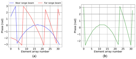
Figure 1.
Phase tapers (in radians) of the array elements (a) for the near range beam of 120 km ground swath (blue curve) scenario and the far range beam of 120 km ground swath scenario (red curve) and (b) for 240 km ground swath scenario.

Figure 2.
Achieved sector beams in elevation: (a) two beams, which cover 120 km ground swath each, and (b) one beam, which covers 240 km ground swath as function of look angle. The look angle span between near and far range is highlighted for each beam. The positions of the range ambiguities of the scatterer at near range (circle marker) and of the scatterer at far range (x marker) are shown.
Once the antenna beam in elevation is defined, the PRF for the low PRF ambiguous mode and the PRI sequence for the staggered (high PRF) ambiguous mode, along with the pulse width, should be defined to ensure the desired duty cycle. For the low PRF ambiguous mode, the exact value of the PRF is selected from the timing diagram as shown in Figure 3. The selected PRF for the near range beam of a 120 km ground swath is 865 Hz (blue line in Figure 3), which is 3.2 times smaller than the Doppler bandwidth (i.e., ), and the corresponding pulse width is 231 µs to ensure the 20% duty cycle. We chose a = 565 Hz (red line in Figure 3) for the far range beam of a 120 km ground swath, which is 5 times smaller than the Doppler bandwidth, and a pulse width of 354 µs to ensure a 20% duty cycle. Alternatively, we can select a higher PRF for this case, = 767 Hz, which is 3.6 times smaller than the Doppler bandwidth, and eliminate the nadir echo return by exploiting the waveform-encoded SAR concept, i.e., alternating, e.g., up- and down-chirps on transmit and removing the nadir echo within a postprocessing step [41,42]. In this case, we can transmit a shorter pulse with 261 µs to maintain the 20% duty cycle. Finally, we can select a = 363 Hz to image a 240 km swath width in the ground, which needs the transmission of a much longer pulse with 551 µs to achieve a duty cycle of 20%. The lower the PRF value, the higher the AASR. Specifically, an = 1.62 dB is obtained for the near range beam of a 120 km ground swath, an = 4.38 dB and an = 2.46 dB are obtained for the far range beam of a 120 km ground swath with 565 Hz and = 767 Hz, respectively, and an = 6.83 dB is obtained for the 240 km ground swath scenario.

Figure 3.
Timing diagram for a duty cycle of 20% The orange and black zones represent transmit and nadir interferences, respectively. The blue line represents the near range ground swath of 120 km, the red line represents the far range ground swath of 120 km, and the green line represents the 240 km ground swath.
Now that the PRF has been selected, we can exploit the azimuth displacement expression of the azimuth ambiguities to determine whether the azimuth ambiguities of the ground scatterers will cause false alarms within the swath while monitoring EEZs. At a given azimuth distance, , the smallest azimuth ambiguity order due to land scatterers observable within the swath is [40]
where is the ambiguity order and is the floor function, i.e., the largest integer not greater than the argument of the function. We obtain () for = 22 km, which is the outer limit of the territorial sea, i.e., the beginning of the EEZs, and a = (or = 363 Hz for the 240 km ground swath scenario, which is 8 times smaller than ). As a result, false alarms due to azimuth ambiguities of ground scatterers with ambiguity order are not expected. We can even operate our mode 12 km from the coast in the azimuth direction, avoiding ambiguities up to the third order when = (i.e., the 24th ambiguity order when = 363 Hz).
For the staggered (high PRF) ambiguous mode, three different sequences are designed for the two 120 km beams and the 240 km beam, so that the sequence’s mean duty cycle is equal to 20% and two consecutive samples are never missed in the raw azimuth signal for each slant range [31]. A sequence of 29 PRIs is designed with = 3740 Hz, which is greater than the Doppler bandwidth and a pulse width 56 µs is selected to ensure a mean duty cycle of 20% for the near range beam of a 120 km ground swath. For the far range beam of a 120 km ground swath, a sequence of 33 PRIs with nearly the same as the near range beam, = 3713 Hz, is designed and the same pulse width of 56 µs is selected. A PRI sequence of 30 PRIs at = 3689 Hz is designed for the 240 km ground swath, with a pulse width of 57 µs chosen to ensure a mean duty cycle of 20%. We achieve the same duty cycle for the staggered (high PRF) ambiguous mode, ensuring the same detection performance as the low PRF ambiguous mode while transmitting a pulse that is 4–10 times shorter, according to the discussions in Section 3.2.
Now that the PRF and pulse width have been determined, the NESZ is calculated using (10) and the antenna pattern in elevation depicted in Figure 2. Figure 4a,b show the NESZ as a function of ground range for the two beams that image a 120 km ground swath each and for the beam that images a 240 km ground swath, respectively. We observe that NESZ ranges from −9.3 dB to 3.2 dB, implying that the clutter contribution is negligible in comparison to thermal noise in accordance with [20].
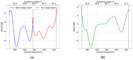
Figure 4.
NESZ as function of ground range (incidence angle) for system parameters shown in Table 2 and Table 3 and a duty cycle of 20% (a) for the near range beam (blue curve) and far range beam (red curve) that image 120 km ground swath each and (b) the beam that covers a 240 km ground swath. The 120 km ground swaths and the 240 km ground swath are highlighted.
Using (5), we calculate the PD of a small ship of 21 m × 6 m size as a function of ground range, as shown in Figure 5, for the beams of Figure 2, based on the NESZ values shown in Figure 4. In all cases, we assume that the number of false alarms per million km2 is 103 (i.e., ), which corresponds to a × 10−7 according to (9). We note that the varies due to the NESZ variation within the swath. Furthermore, we observe that the mean value of the PD for the two sector beams of 120 km is in the range = 0.97–0.99, and the worst PD is achieved at the near range of the first beam due to the antenna pattern. The mean value of for the 240 km sector beam is = 0.8, and the worst probability of detection is obtained at near and far ranges due to the antenna pattern and is in the order of = 0.43. Better detection performances are obtained for ships larger than 21 m × 6 m size, even though they are not reported here for brevity. Specifically, for a medium ship of 40 m × 8 m size we have a probability of detection of approximately 1 over the whole swath even for the 240 km ground swath scenario for the same × 10−7.
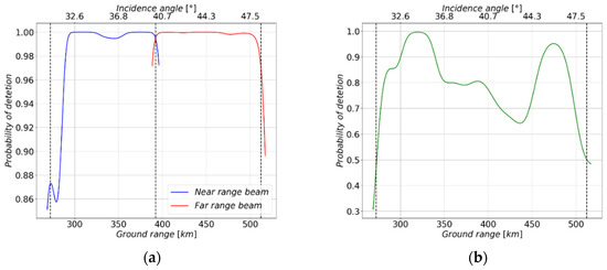
Figure 5.
Probability of detection of a small ship of 21 m × 6 m size (a) for the near range beam (blue curve) and far range beam (red curve), which cover a 120 km ground swath each, and (b) for the beam, which covers a 240 km ground swath. The 120 km ground swaths and the 240 km ground swath are highlighted.
In order to give the reader an idea of how the SAR images for the presented ambiguous modes look, we provide a simulated image based on a spotlight TerraSAR-X image with resolution cell of 2 m2 and NESZ < −20 dB acquired over South Indonesia (Figure 6a). A simulated SAR image, as if acquired with one of the ambiguous modes, can be generated by artificially adding noise to the data and would look like the image in Figure 6b, where some details of the ship structure, particularly for small ships, are no longer visible. The simulated SAR image takes into account the worse NESZ, i.e., NESZ = 2 dB, as a result of the wide beam in elevation and the increased sea clutter level as a result of higher ambiguities (see Table 1). The intensity of the simulated SAR image is compared with the threshold T selected in accordance with (5) to guarantee the detection of a small ship of 21 m × 6 m size with a × 10−7. Figure 6c shows the detection map of pixels that have exceeded the threshold, with the superimposed extracted region of interest represented by red squares after pixel clustering. We notice that all nine ships have been detected. Please keep in mind that azimuth ambiguities of ships which might appear in the low PRF ambiguous mode are not taken into account here.

Figure 6.
(a) Reference TerraSAR-X image in spotlight mode, (b) simulated image as if acquired with one of the two ambiguous modes that considers the worse NESZ and the increased sea clutter level due to the higher ambiguity level, and (c) the detection map with the regions of interest indicated by the red boxes.
Another important aspect to consider for the low PRF ambiguous mode is the presence of range ambiguities from other large ships within and out of the swath due to the wide antenna pattern in elevation and its relatively high sidelobes. Based on the PRF values chosen (see Figure 3), we compute the position of the range ambiguities for the three beams. We use (8) to calculate the probability that the range ambiguity of a large ship will exceed a given threshold chosen to ensure the desired PFA and PD, but with a larger resolution cell because the ships’ range ambiguities are smeared:
where is the number of smearing cells along azimuth of the pth order range ambiguity due to range cell migration and assuming that the number of smearing cells in range is [40,44]. The average signal to noise ratio of the range ambiguities used for the computation of the PD in (8) is defined as
where the and the parameters of a large ship in stripmap mode (see Table I of [20]), and = 5.40, are used for the computation of the in (7) and of the parameter, and Equation (10) is used for the computation of the with the corresponding slant ranges and incidence angles of the range ambiguities. The obtained probability of detection could then be compared to the desired probability of false alarm, taking into account that the number of false alarms resulting from range ambiguities also depends on the actual number of large ships in and around the observed scene. If the PD of the range ambiguities is higher than the PFA, the waveform and azimuth phase codes concepts discussed in Section 2 could be employed to further smear the range ambiguities even more in order to avoid possible additional false alarms. Because of the smearing (i.e.,), smaller values of and are expected when compared to the used values, which refer to a nominal resolution of 3 m × 3 m (i.e., stripmap mode), resulting in a lower and smaller . As a result, the obtained PD is optimistic when compared to the effective value, resulting in a more conservative decision to employ the waveform-encoded concepts. The probability of detection of the range ambiguity of a medium or small ship is lower than that of the range ambiguity of a large ship, which is why a large ship is considered in the following analysis. For the considered scenarios, no range ambiguities due to the previous transmitted pulse are expected, but only range ambiguities due to the succeeding transmitted pulse, as shown by the markers in Figure 2. In accordance with the above discussion, we compute the PD of the first- and second-order range ambiguities of a large ship of 300 m × 20 m size for a threshold that guarantees the detection of a small ship (i.e., 21 m × 6 m) with a within the swath and PD as shown in Figure 5. The smearing of the first-order range ambiguities ranges from cells for = 865 Hz (i.e., near range beam of a 120 km ground swath) to cells for = 363 Hz (i.e., 240 km ground swath beam), and the smearing of the second-order range ambiguities ranges from cells for = 865 Hz to cells for = 363 Hz. Table 4 reports the obtained PD using (8). We note that the highest PD is in the order 10−3 for the near range beam of a 120 km ground swath, which is much higher than the desired . To avoid range ambiguities exceeding the detection threshold, it is recommended that the waveform-encoded and azimuth phase code concepts discussed in Section 2 be used for this scenario. Now, the smearing in range of the first-order range ambiguities will be in the order of cells because of the alternation of the up- and down-chirps and in azimuth will be in the order of cells because of the “Doppler-matched” azimuth phase code [43,44]. For the far range beam of a 120 km ground swath and for the 240 km ground swath the highest PD is in the order of 10−7 comparable to the desired . Using waveform-encoded concepts for these scenarios is probably not required, because the computed PD is more optimistic than the effective PD. In all cases, the PD of the second-order range ambiguities of a large ship is smaller than the desired PFA, and thus no impact on detection performance is expected.
Table 4.
Probability of detection of the first- and second-order range ambiguities of a large ship of 300 m × 20 m size for the different beams.
It is worth noting that exploiting waveform-encoded and azimuth phase code concepts will also avoid false alarms caused by potential range ambiguities of far land scatterers.
Comparison with the ScanSAR
For comparison, we compute the rough detection performance of TerraSAR-X for a small ship in ScanSAR mode (i.e., 100 km swath), which has a nominal NESZ −19 dB and a resolution cell of 18.5 m × 5 m [46]. Because of the better NESZ compared to the ambiguous modes, for the ScanSAR mode it is expected that the sea clutter contribution will be the dominant component of the disturbance, i.e., it will be well above the noise level. We therefore assume that the sea clutter follows a K distribution with scale parameter and shape parameter [59,60]; thus, the clutter to noise ratio is
The shape parameter defines the spikiness of the sea clutter and it varies from 0.1, corresponding to very spiky data, to greater than 20, corresponding to approximately Rayleigh distributed data. In the absence of a statistical characterization of ships from the X-band system in ScanSAR mode, we conservatively assume that they follow a log-normal distribution with the same parameters as in the stripmap mode with nominal resolution 3 m × 3 m (see Table I of [20]). The statistical proprieties of the ship, as discussed in previous sections, vary with resolution. As a result, it is unlikely that a small ship of 21 m × 6 m size, which occupies 14 resolution cells in stripmap mode, will have the same SNR = 13.6 dB in ScanSAR mode, where the small ship occupies 1 resolution cell. Thus, the computed PD will be significantly higher than the effective value. For the computation of the SNR, Equation (6) along with and = 1.490 (from Table I of [20]) are used. To calculate the detection performance, we set a global threshold that ensures the desired PFA and then declare any pixel intensities above this threshold as targets of interest. Ref. [60] gives the closed-form expression of the PFA as a function of the detection threshold T, scale, and shape parameter for a K-distributed background:
where is the modified Bessel function of order . For the probability of detection, we use the same closed-form expression in (8) with , NESZ = −19 dB, and SNR = 13.6 dB. We assume here that the scale and shape parameters of the sea clutter are known a priori, which is not in general the case. As a result, it is far more common to employ a CFAR detector that estimates the parameter distribution, resulting in a PD lower than the computed one. Figure 7 shows the PD of the same small ship (i.e., 21 m × 6 m size) as a function of the CNR and shape parameter for × 10−7. We note that for all case studies the PD is below 0.3, even for a CNR = 0 dB (i.e., dB) and shape parameter . The achieved PD is therefore much lower than the PD obtained with the ambiguous modes, which was equal to 0.97 and 0.8 for the 120 km and 240 km ground swath cases, respectively.

Figure 7.
Probability of detection of small ship of 21 m × 6 m size in ScanSAR mode as a function of the CNR and shape parameter for a × 10−7.
The Wide ScanSAR mode of TerraSAR-X is characterized by a NESZ −15 dB and a resolution cell of 40 m × 7 m size [46]. A small ship of 21 m × 6 m size will occupy a portion of the resolution cell and therefore it will be much harder to detect it.
The “maritime mode” of NovaSAR, which is also based on the ScanSAR mode, has a resolution cell of 13.7 m × 6 m, which is 37 times lower than the proposed ambiguous modes for TerraSAR-X (i.e., the resolution cell ranges from 2.2 m2 to 1.5 m2) and allows for the detection of medium ships with a false alarm rate of 10−7 [37].
5. Conclusions
Two HRWS modes are presented that can be adapted to existing, planned, and future SAR systems to provide additional modes for efficient ship detection across ultra-wide swaths. The two modes image a wide swath employing a wide elevation beam obtained through phase-only tapering and achieve high azimuth resolution. The low PRF ambiguous mode is a stripmap mode with a PRF smaller than the nominal Doppler bandwidth because the azimuth ambiguities of the ship can be tolerated. The staggered (high PRF) ambiguous mode employs a sequence of M distinct PRIs that then repeat periodically because the range ambiguities of the ships are smeared and do not impact the detection performances. Both modes are thought to operate in open sea surveillance where there are no azimuth ambiguities for the low PRF ambiguous mode or range ambiguities for the staggered (high PRF) ambiguous mode from strong ground scatterers that could interfere with ship detection, whereas for coastal areas a conventional SAR, such as a stripmap mode, could be used. The low PRF ambiguous mode requires the use of long pulses in order to achieve a higher duty cycle and, as a result, a better detection performance. Instead, because the mean PRF of the sequence is greater than the nominal Doppler bandwidth, the staggered (high PRF) ambiguous mode does not require the transmission of long pulses to achieve a higher duty cycle. In the examples in this paper, the same detection performance is achieved with the staggered (high PRF) ambiguous mode while transmitting a pulse that is 4–10 times shorter than in the low PRF ambiguous mode. However, the data volume in the staggered (high PRF) ambiguous mode is significantly higher than in the low PRF ambiguous mode, which is why this mode would benefit most from on-board processing. When compared to the low PRF ambiguous mode, the L1 processing step for the staggered (high PRF) ambiguous mode requires some more elaborated processing, such as raw data alignment and interpolation along azimuth.
Knowing the specific SAR architecture and limitations, such as the system’s minimum and maximum selectable pulse width, maximum allowable duty cycle, echo buffer length, minimum and maximum selectable PRF, the system’s ability to change the PRI, and the possibility of on-board processing, will allow us to determine which of the two ambiguous modes is more suitable for ship monitoring.
From the examples in this paper, it is shown that using the ambiguous modes, it is possible to detect small ships (i.e., 21 m × 6 m) by imaging a wide swath of 120 km and 240 km and having a resolution cell of 2 m2, similar to the spotlight mode, with a very low false alarm rate and a detection probability of 0.97 and 0.85, respectively. The comparison of detection performances with the ScanSAR mode, which images a wide swath but has a coarse resolution cell (i.e., 46 times lower than the ambiguous modes) and a better NESZ (i.e., 10 dB higher), demonstrated the significance of resolution for ship detection applications. The probability of detection in the ScanSAR mode of the same ship with the same PFA as for the ambiguous mode is less than 0.3, which is the PD for the optimistic case.
As for the specific application, ship ambiguities can be tolerated, and the system design does not need to follow conventional design principles, which are driven by range and azimuth ambiguities, ensuring wide swath and high resolution at the same time.
In the near future, a TerraSAR-X experimental acquisition is planned to demonstrate the effectiveness of the proposed ambiguous mode. For the experimental acquisition, we must consider the technical constraints (e.g., allowed selectable PRF value, longest selectable pulse width, echo buffer length). As a result, we must adopt some parameters to meet the constraints, which will affect the performance in terms of swath width or detection performance. For TerraSAR-X, the staggered (high PRF) ambiguous mode is preferable to the low PRF ambiguous mode due to the constraints of the echo buffer length and duty cycle.
Other applications that might exploit these modes, such as deformation monitoring using permanent scatterers interferometry, are currently under investigation.
Author Contributions
Conceptualization and methodology, N.U. and M.V.; writing—original draft preparation, N.U.; writing—review and editing, N.U. and M.V. All authors have read and agreed to the published version of the manuscript.
Funding
This research received no external funding.
Informed Consent Statement
Not applicable.
Data Availability Statement
Data sharing is not applicable to this article.
Acknowledgments
The authors would like to acknowledge their colleagues Gerhard Krieger, Ulrich Steinbrecher, and Thomas Kraus for many constructive discussions.
Conflicts of Interest
The authors declare no conflict of interest.
References
- Moreira, A.; Prats-Iraola, P.; Younis, M.; Krieger, G.; Hajnsek, I.; Papathanassiou, K.P. A tutorial on synthetic sperture radar. IEEE Geosci. Remote Sens. Mag. 2013, 1, 6–43. [Google Scholar] [CrossRef] [Green Version]
- Eldhuset, K. An automatic ship and ship wake detection system for spaceborne SAR images in coastal regions. IEEE Trans. Geosci. Remote Sens. 1996, 34, 1010–1019. [Google Scholar] [CrossRef]
- Vachon, P.W.; Campbell, J.; Bjerkelund, C.; Dobson, F.; Rey, M. Ship detection by the RADARSAT SAR: Validation of detection model predictions. Can. J. Remote Sens. 1997, 23, 48–59. [Google Scholar] [CrossRef]
- Brusch, S.; Lehner, S.; Fritz, T.; Soccorsi, M.; Soloviev, A.; van Schie, B. Ship surveillance with TerraSAR-X. IEEE Trans. Geosci. Remote Sens. 2001, 49, 1092–1103. [Google Scholar] [CrossRef]
- Crisp, D.J. The State-of-the-Art in Ship Detection in Synthetic Aperture Radar Imagery; Defence Science and Technology Organisation Salisbury (Australia) Info Sciences Lab.: Edinburgh, Australia, 2004.
- Lombardo, P.; Sciotti, M. Segmentation-based technique for ship detection in SAR images. IEE Proc. Radar Sonar Navig. 2001, 148, 147–159. [Google Scholar] [CrossRef]
- Pastina, D.; Fico, F.; Lombardo, P. Detection of ship targets in COSMO-SkyMed SAR images. In Proceedings of the 2011 IEEE RadarCon (RADAR), Kansas City, MO, USA, 23–27 May 2011; pp. 928–933. [Google Scholar]
- Martorella, M.; Berizzi, F.; Pastina, D.; Lombardo, P. Exploitation of Cosmo SkyMed SAR images for maritime traffic surveillance. In Proceedings of the 2011 IEEE RadarCon (RADAR), Kansas City, MO, USA, 23–27 May 2011; pp. 113–117. [Google Scholar]
- Greidanus, H.; Alvarez, M.; Santamaria, C.; Thoorens, F.-X.; Kourti, N.; Argentieri, P. The SUMO ship setector slgorithm for satellite sadar images. Remote Sens. 2017, 9, 246. [Google Scholar] [CrossRef] [Green Version]
- Jiang, Q.; Wang, S.; Ziou, D.; El Zaart, A.; Rey, M.T.; Benie, G.B.; Henschel, M. Ship detection in RADARSAT SAR imagery. In Proceedings of the SMC’98 Conference Proceedings. 1998 IEEE International Conference on Systems, Man, and Cybernetics (Cat. No.98CH36218), San Diego, CA, USA, 14 October 1998; Volume 5, pp. 4562–4566. [Google Scholar]
- Iervolino, P.; Guida, R. A novel ship detector based on the generalized-likelihood ratio test for SAR imagery. IEEE J. Sel. Top. Appl. Earth Obs. Remote Sens. 2017, 10, 3616–3630. [Google Scholar] [CrossRef] [Green Version]
- Liao, M.; Wang, C.; Wang, Y.; Jiang, L. Using SAR images to detect ships from sea clutter. IEEE Geosci. Remote Sens. Lett. 2008, 5, 194–198. [Google Scholar] [CrossRef]
- Bentes, C.; Velotto, D.; Lehner, S. Analysis of ship size detectability over different TerraSAR-X modes. In Proceedings of the 2014 IEEE Geoscience and Remote Sensing Symposium, Quebec City, QC, Canada, 13–18 July 2014; pp. 5137–5140. [Google Scholar]
- Vachon, P.W.; Wolfe, J.; Greidanus, H. Analysis of Sentinel-1 marine applications potential. In Proceedings of the 2012 IEEE International Geoscience and Remote Sensing Symposium, Munich, Germany, 22–27 July 2012; pp. 1734–1737. [Google Scholar]
- Greidanus, H.; Clayton, P.; Indregard, M.; Staples, G.; Suzuki, N.; Vachoir, P.; Wackerman, C.; Tennvassas, T.; Mallorqui, J.; Kourti, N.; et al. Benchmarking operational SAR ship detection. In Proceedings of the IGARSS 2004. 2004 IEEE International Geoscience and Remote Sensing Symposium, Anchorage, AK, USA, 20–24 September 2004; Volume 6, pp. 4215–4218. [Google Scholar]
- Gierull, C.H.; Sikaneta, I. A compound-plus-noise model for improved vessel detection in non-gaussian SAR imagery. IEEE Trans. Geosci. Remote Sens. 2018, 56, 1444–1453. [Google Scholar] [CrossRef]
- Krecke, J.; Villano, M.; Ustalli, N.; Austin, A.C.M.; Cater, J.E.; Krieger, G. Detecting ships in the New Zealand Exclusive Economic Zone: Requirements for a dedicated amallSat SAR mission. IEEE J. Sel. Top. Appl. Earth Obs. Remote Sens. 2021, 14, 3162–3169. [Google Scholar] [CrossRef]
- Schwarz, E.; Krause, D.; Voinov, S.; Daedelow, H.; Lehner, S. Near real time applications for maritime situational awareness. In Proceedings of the Fourth International Conference on Remote Sensing and Geoinformation of Environment (RSCY2016), Paphos, Cyprus, 4–8 April 2016. [Google Scholar]
- Voinov, S.; Schwarz, E.; Krause, D.; Berg, M. Identification of SAR detected targets on sea in near real time applications for maritime surveillance. Free. Open Source Softw. Geospat. (FOSS4G) Conf. Proc. 2016, 16, 1. [Google Scholar] [CrossRef]
- Ustalli, N.; Krieger, G.; Villano, M. A low-power, ambiguous synthetic aperture radar concept for continuous ship monitoring. IEEE J. Sel. Top. Appl. Earth Obs. Remote Sens. 2022, 15, 1244–1255. [Google Scholar] [CrossRef]
- Curlander, J.C.; McDonough, R.N. Synthetic Aperture Radar Systems and Signal Processing; Wiley: Hoboken, NJ, USA, 1991. [Google Scholar]
- Tomiyasu, K. Conceptual performance of a satellite borne, wide swath synthetic aperture radar. IEEE Trans. Geosci. Remote Sens. 1981, GE-19, 108–116. [Google Scholar] [CrossRef]
- De Zan, F.; Monti Guarnieri, A. TOPSAR: Terrain observation by progressive scans. IEEE Trans. Geosci. Remote Sens. 2006, 44, 2352–2360. [Google Scholar] [CrossRef]
- Goodman, N.; Rajakrishna, D.; Stiles, J. Wide swath, high resolution SAR using multiple receive apertures. In Proceedings of the IEEE 1999 International Geoscience and Remote Sensing Symposium. IGARSS’99 (Cat. No. 99CH36293), Hamburg, Germany, 28 June–2 July 1999; Volume 3, pp. 1767–1769. [Google Scholar]
- Gebert, N.; Krieger, G.; Moreira, A. Digital beamforming for HRWS-SAR imaging: System design, performance and optimization strategies. In Proceedings of the 2006 IEEE International Symposium on Geoscience and Remote Sensing, Denver, CO, USA, 31 July–4 August 2006; pp. 1836–1839. [Google Scholar]
- Krieger, G.; Gebert, N.; Moreira, A. Unambiguous SAR signal reconstruction from nonuniform displaced phase center sampling. IEEE Geosci. Remote Sens. Lett. 2004, 1, 260–264. [Google Scholar] [CrossRef] [Green Version]
- Krieger, G.; Gebert, N.; Younis, M.; Bordoni, F.; Patyuchenko, A.; Moreira, A. Advanced concepts for ultra-wide-swath SAR imaging. In Proceedings of the EUSAR, Friedrichshafen, Germany, 2–5 June 2008. [Google Scholar]
- Freeman, A.; Krieger, G.; Rosen, P.; Younis, M.; Johnson, W.T.K.; Huber, S.; Jordan, R.; Moreira, A. SweepSAR: Beam-forming on receive using a reflector-phased array feed combination for spaceborne SAR. In Proceedings of the IEEE Radar Conference, Pasadena, CA, USA, 4–8 May 2009. [Google Scholar]
- Villano, M.; Krieger, G.; Moreira, A. Staggered SAR: High-resolution wide-swath imaging by continuous PRI variation. IEEE Trans. Geosci. Remote Sens. 2014, 52, 4462–4479. [Google Scholar] [CrossRef]
- Villano, M.; Krieger, G.; Moreira, A. A novel processing strategy for staggered SAR. IEEE Geosci. Remote Sens. Lett. 2014, 11, 1891–1895. [Google Scholar] [CrossRef]
- Villano, M. Staggered Synthetic Sperture Radar. Ph.D. Thesis, Karlsruhe Institute of Technology, Wessling, Germany, 2016. [Google Scholar]
- Villano, M.; Krieger, G.; Jäger, M.; Moreira, A. Staggered SAR: Performance analysis and experiments with real Data. IEEE Trans. Geosci. Remote Sens. 2017, 55, 6617–6638. [Google Scholar] [CrossRef]
- Ustalli, N.; Villano, M.; Krieger, G. Design of a low-cost synthetic aperture radar for continuous ship monitoring. In Proceedings of the 2021 IEEE International Geoscience and Remote Sensing Symposium IGARSS, Brussels, Belgium, 11–16 July 2021; pp. 7872–7875. [Google Scholar]
- Iervolino, P.; Cohen, M.; Guida, R.; Whittaker, P. Ship-detection in SAR imagery using low pulse repetition frequency radar. In Proceedings of the EUSAR 2014; 10th European Conference on Synthetic Aperture Radar, Berlin, Germany, 3–5 June 2014; pp. 1–4. [Google Scholar]
- Whittaker, P.; Doodyb, S.; Cohenb, M.; Schwarza, B.; Burbidgeb, G.; Birda, R. NovaSAR-1—Early mission achievements. In Proceedings of the EUSAR 2021, 13th European Conference on Synthetic Aperture Radar, online, 29 March–1 April 2021; pp. 1–4. [Google Scholar]
- Márquez-Martínez, J.; Cohen, M.; Doody, S.; Lau-Semedo, P.; Larkins, A. Next generation low cost SAR payloads: Novasar-S and beyond. In Proceedings of the 2017 IEEE International Geoscience and Remote Sensing Symposium (IGARSS), Fort Worth, TX, USA, 23–28 July 2017; pp. 3848–3851. [Google Scholar]
- Cohen, M.; Larkins, A.; Semedo, P.L.; Burbidge, G. NovaSAR-S low cost spaceborne SAR payload design, development and deployment of a new benchmark in spaceborne radar. In Proceedings of the 2017 IEEE Radar Conference (RadarConf), Seattle, WA, USA, 8–12 May 2017; pp. 0903–0907. [Google Scholar]
- Freeman, A.; Johnson, W.T.K.; Huneycutt, B.; Jordan, R.; Hensley, S.; Siqueira, P.; Curlander, J. The “Myth” of the minimum SAR antenna area constraint. IEEE Trans. Geosci. Remote Sens. 2000, 38, 20–324. [Google Scholar] [CrossRef] [Green Version]
- Freeman, A. Design principles for smallsat SARs. In Proceedings of the 32nd Annual AIAA/USU Conference on Small Satellites, Logan, UT, USA, 3–8 August 2018. [Google Scholar]
- Li, F.K.; Johnson, W.T.K. Ambiguities in spaceborne synthetic aperture radar systems. IEEE Trans. Aerosp. Electron. Syst. 1983, 19, 389–397. [Google Scholar] [CrossRef]
- Villano, M.; Krieger, G.; Moreira, A. Nadir echo removal in synthetic aperture radar via waveform diversity and dual-focus post-processing. IEEE Geosci. Remote Sens. Lett. 2018, 15, 719–723. [Google Scholar] [CrossRef]
- Jeon, S.-Y.; Villano, M.; Kraus, T.; Steinbrecher, U.; Krieger, G. Experimental demonstration of nadir echo removal in SAR using waveform diversity and dual-focus postprocessing. IEEE Geosci. Remote Sens. Lett. 2021, 19, 4015605. [Google Scholar] [CrossRef]
- Villano, M.; Peixoto, M.N.; Dell’Amore, L.; Jeon, S.-Y.; Ustalli, N.; Krecke, J.; Mittermayer, J.; Krieger, G.; Moreira, A. NewSpace SAR: Disruptive concepts for cost-effective SAR system design. In Proceedings of the EUSAR 2021; 13th European Conference on Synthetic Aperture Radar, online, 29 March–1 April 2021; pp. 1–6. [Google Scholar]
- Ustalli, N.; Villano, M. Impact of ambiguity statistics on information retrieval for conventional and novel SAR modes. In Proceedings of the 2020 IEEE Radar Conference (RadarConf20), Florence, Italy, 21–25 September 2020; pp. 1–6. [Google Scholar]
- Roth, A.; Marschalk, U.; Winkler, K.; Schättler, B.; Huber, M.; Georg, I.; Künzer, C.; Dech, S. Ten years of experience with scientific TerraSAR-X data utilization. Remote Sens. 2018, 10, 1170. [Google Scholar] [CrossRef] [Green Version]
- TerraSAR-X. Available online: https://sss.terrasar-x.dlr.de/docs/TX-GS-DD-3302.pdf (accessed on 20 April 2022).
- Shnidman, D.A. Calculation of probability of detection for log-normal target fluctuations. IEEE Trans. Aerosp. Electron. Syst. 1991, 27, 172–174. [Google Scholar] [CrossRef]
- Villano, M.; Krieger, G.; Moreira, A. Advanced spaceborne SAR systems with planar antenna. In Proceedings of the 2017 IEEE Radar Conference (RadarConf), Seattle, WA, USA, 8–12 May 2017; pp. 152–156. [Google Scholar]
- Touzi, R.; Charbonneau, F.J.; Hawkins, R.K.; Vachon, P.W. Ship detection and characterization using polarimetric SAR. Can. J. Remote Sens. 2004, 30, 552–559. [Google Scholar] [CrossRef]
- Yeremy, M.; Campbell, J.W.M.; Mattar, K.; Potter, T. Ocean surveillance with polarimetric SAR. Can. J. Remote Sens. 2001, 27, 328–344. [Google Scholar] [CrossRef]
- Sciotti, M.; Pastina, D.; Lombardo, P. Exploiting the polarimetric information for the detection of ship targets in non-homogeneous SAR images. In Proceedings of the IEEE 2002 International Geoscience and Remote Sensing Symposium (IGARSS’02), Toronto, ON, Canada, 24–28 June 2002; Volume 3, pp. 1911–1913. [Google Scholar]
- Han, Z.; Chong, J. A review of ship detection algorithms in polarimetric SAR images. In Proceedings of the 7th International Conference on Signal Processing, 2004. Proceedings. ICSP’04. 2004, Beijing, China, 31 August–4 September 2004; Volume 3, pp. 2155–2158. [Google Scholar]
- Velotto, D.; Nunziata, F.; Migliaccio, M.; Lehner, S. Dual-polarimetric TerraSAR-X SAR data for target at sea observation. IEEE Geosci. Remote Sens. Lett. 2013, 10, 1114–1118. [Google Scholar] [CrossRef]
- Crisp, D.J. A ship detection system for RADARSAT-2 dual-pol multi-look imagery implemented in the ADSS. In Proceedings of the 2013 International Conference on Radar, Adelaide, SA, Australia, 9–12 September 2013; pp. 318–323. [Google Scholar]
- EO-ALERT-Next generation satellite processing chain for rapid civil alert. Available online: http://eo-alert-h2020.eu/ (accessed on 25 April 2022).
- Kerr, M.; Tonetti, S.; Carnara, S.; Bravo, J.I.; Hinz, R.; Latorre, A.; Membibre, F.; Ramos, A.; Wiehle, S.; Koudelka, O.; et al. EO-Alert: A satellite architecture for detection and monitoring of extreme events in real time. In Proceedings of the 2021 IEEE International Geoscience and Remote Sensing Symposium IGARSS, Brussels, Belgium, 11–16 July 2021; pp. 168–171. [Google Scholar]
- Wiehle, S.; Günzel, D.; Tings, B. SAR satellite on-board ship, wind, and sea state detection. In Proceedings of the 2021 IEEE International Geoscience and Remote Sensing Symposium IGARSS, Brussels, Belgium, 11–16 July 2021; pp. 8289–8292. [Google Scholar]
- Breit, H.; Mandapati, S.; Balss, U. An FPGA/MPSoC based low latency onboard SAR processor. In Proceedings of the 2021 IEEE International Geoscience and Remote Sensing Symposium IGARSS, Brussels, Belgium, 11–16 July 2021; pp. 5159–5162. [Google Scholar]
- Watts, S. Radar detection prediction in sea clutter using the compound K-distribution model. IEE Proc. 1985, 132, 613–620. [Google Scholar] [CrossRef]
- Watts, S. Radar detection prediction in K-distributed sea clutter and thermal noise. IEEE Trans. Aerosp. Electron. Syst. 1987, AES-23, 40–45. [Google Scholar] [CrossRef]
Publisher’s Note: MDPI stays neutral with regard to jurisdictional claims in published maps and institutional affiliations. |
© 2022 by the authors. Licensee MDPI, Basel, Switzerland. This article is an open access article distributed under the terms and conditions of the Creative Commons Attribution (CC BY) license (https://creativecommons.org/licenses/by/4.0/).