Abstract
Persistent scatterer interferometry (PSI) is a group of advanced interferometric synthetic aperture radar (SAR) techniques used to measure and monitor terrain deformation. Sentinel-1 has improved the data acquisition throughout and, compared to previous sensors, increased considerably the differential interferometric SAR (DInSAR) and PSI deformation monitoring potential. The low density of persistent scatterer (PS) in non-urban areas is a critical issue in DInSAR and has inspired the development of alternative approaches and refinement of the PS chains. This paper proposes two different and complementary data-driven procedures to obtain terrain deformation maps. These approaches aim to exploit Sentinel-1 highly coherent interferograms and their short revisit time. The first approach, called direct integration (DI), aims at providing a very fast and straightforward approach to screen-wide areas and easily detects active areas. This approach fully exploits the coherent interferograms from consecutive images provided by Sentinel-1, resulting in a very high sampling density. However, it lacks robustness and its usability lays on the operator experience. The second method, called persistent scatterer interferometry geomatics (PSIG) short temporal baseline, provides a constrained application of the PSIG chain, the CTTC approach to the PSI. It uses short temporal baseline interferograms and does not assume any deformation model for point selection. It is also quite a straightforward approach, which improves the performances of the standard PSIG approach, increasing the PS density and providing robust measurements. The effectiveness of the approaches is illustrated through analyses performed on different test sites.
1. Introduction
Synthetic aperture radar (SAR) is an extensive tool able to measure different aspects of the illuminated surface such as topography [1], changes over time [2], soil moisture [3] and surface displacements [4]. In the last 25 years, the differential SAR interferometry technique (DInSAR) has been widely used as a tool to map and measure ground displacements. Over these years, the development of processing tools and the increasing availability of data have turned the DInSAR techniques into an operative and reliable tool for mapping and monitoring geohazards [5], such as earthquakes [6,7], landslides [8], mining activities [9] or subsidences [10]. In particular, the advanced DInSAR techniques (A-DInSAR), a set of techniques that make use of stacks of SAR images, might be exploited to obtain very high-precision (mm order) displacement measurements, while covering extensive areas of terrain [11]. These unique capabilities have motivated the setup of several monitoring programs at regional [12,13], national [14], and even European level [15], and an intensive research effort to improve their reliability and provide key inputs for geohazard risk managers [16,17,18]. However, despite these efforts, there is still a significant bias between the amount of useful information provided by single interferograms and the results provided by these advanced methods.
The main outputs of A-DInSAR techniques are twofold: (i) the deformation velocity maps providing yearly rates of movement for each measure point and (ii) time series of ground deformation containing information on the temporal evolution of deformation of such points. These two outputs, together with the high density of measures that A-DInSAR usually provides, are the key inputs for understanding the behavior of the studied phenomena [19]. However, as a remote geodetic technique, A-DInSAR is affected by different interfering signals such as noise, atmospheric disturbances, signals not related with the target of the analysis and outliers that must be properly treated and removed [20,21]. One of the most critical aspects is the ambiguous nature of the interferometric phase [22]. The interferometric phase contains information about the changes on the two-way travel distance of the signal (antenna–object–antenna) between two acquisitions. However, the phase is compressed or wrapped in the interval [–π, π] [22], thus the information is kept at wavelength level, i.e., it only provides information about changes at wavelength level rather than the information about the full path. Consequently, one of the main sources of error of the A-DInSAR techniques is the process of recovering the absolute values of the phase. This process is known as phase unwrapping, and it is an ill-posed problem. Many papers dealing with this topic can be found in the literature, e.g., see [22,23,24,25]. However, none of the methods is robust enough. Most of the A-DInSAR approaches address this problem by trying to minimize or remove the error sources before the phase unwrapping step by working only with points with a low level of noise [26], removing the main atmospheric signals [27], estimating and removing the topographic component [28], or by modelling part of the displacement component from the interferograms [21]. See [11] for a comprehensive review of these methods.
The new C-band sensor on-board the Sentinel-1 (S-1) A and B satellites, launched in 2014 and 2016, respectively, is a significant improvement in SAR interferometry. S-1 has improved the data acquisition throughout and, compared to previous sensors, considerably increased the DInSAR and A-DInSAR deformation monitoring potential [29]. Firstly, they provide higher resolution data compared to previous C-band sensors. Secondly, the high temporal acquisition frequency (6–12 days in a major part of the world), the continuous acquisition policy, and the free of charge image availability has allowed the S-1 satellites to become an operative tool for displacement mapping and monitoring [29]. This is confirmed by the high number of papers produced in the first four years of the whole constellation addressing different monitoring applications such as landslides [5,18,30,31], volcanoes [32,33], subsidence [34,35], or mining [36,37]. Moreover, the large proportion of available data has resulted in the development of advanced products aiming at early warning support [18] or risk management [16]. From the processing point of view, a significant improvement is the availability of 6-day C-band interferograms that provide high coherent signal in places where it was not possible with the previous sensors, e.g., low vegetation fields, dry but non-solid areas, areas with relatively fast displacements, etc. This has improved the A-DInSAR performances in general, mitigating the effects of the phase unwrapping error in many cases, allowing the improvement of the monitoring capabilities in non-urban areas, and promoting a better understanding of the measured phenomena. However, S-1 has also brought in challenging issues such as the management of a huge volume of data [38], the processing of these data [38], and the analysis of the results [39]. These challenging issues have in turn brought in strong efforts in research. A part of the research has been devoted to the development of tools at the processing level addressing two main issues: data ingestion and automation [40,41]. There has also been significant effort at the post-processing level with the development of tools and procedures to provide semi-automatic data analysis and to transform standard A-DInSAR results into more understandable products for end-users [18,39]. Moreover, the capability of monitoring areas once inaccessible with previous sensors has brought in new signal components. It can be observed that S-1 interferograms also unfold a systematic signal in highly coherent points, especially in short temporal baseline interferograms, which cannot be explained by the topographic or atmospheric phase contributions and can significantly affect the deformation measurements. The understanding of the source of this signal and its modelling is also a current research topic [42]. Finally, although the strong potentials of the high coherent interferograms provided by Sentinel-1 constellation, there has not been a strong development on the automatic exploitation of them.
In this paper, we describe two different and complementary A-DInSAR approaches for exploiting S-1 data for deformation measurement and monitoring purposes: the direct integration, which provides a very straightforward, semi-automated approach to detect active deformation areas, and a short temporal baseline approach based on the PSIG chain. These approaches provide easy and fast procedures to fully exploit the temporal revisit time of the S-1 constellation and to provide different levels of robustness for a wide number of applications. The first one is a powerful tool to point the areas to be analyzed by the second one. Following the introduction, the paper starts with the description of the two proposed approaches, and then, it shows results obtained on three different sites for different applications. The main pros and cons of each approach are discussed, comparing some of the results with those obtained by means of a standard A-DInSAR approach. Finally, in the wake of the analyses performed, some conclusions are provided.
2. The Sentinel-1 A-DInSAR Procedures
This section describes the two A-DInSAR procedures used to derive the displacement velocity and time series of deformation. The proposed procedures can be applied to data acquired by any satellite SAR sensor, over any scale. However, optimal performance is achieved with S-1 data.
The phase difference between two different SAR acquisitions, named interferometric phase, can be written as:
where is the actual phase difference due to change in position of the point of interest, is the phase difference due to the change in the atmospheric column between the first and second acquisition, is the phase difference due to topography, and is the phase difference mainly caused by the change of the physical properties of the measured pixel. Finally, k is the wrapping constant that is estimated in the unwrapping step. When a digital elevation model (DEM) is available, the can be simulated and almost removed from the original interferometric phase. The result of these steps is a new interferogram, the differential interferogram, where ideally the displacement signal is usually significant compared to the other components. The proposed approaches address the estimation of the displacement component through different methods. Two data-driven procedures are proposed: the direct integration (DI) and the PSIG short temporal baseline subset method (PSIG-STB). In this work, we are trying to identify which approach works best for different areas, which in turn, depends on many factors such as topography, humidity, vegetation, etc. The low PS density in non-urban areas encouraged the development of complementary techniques to PSI.
2.1. Direct Integration Approach
The DI procedure is a fast and unsupervised approach to map and monitor active areas in remote and natural environments. This approach provides a rapid and simple solution to screen-wide areas and to map and analyze the evolution of relatively fast and local movements. Compared to standard A-DInSAR approaches, it provides a very high sampling density also in areas where it is not common to have measures. The idea of the DI approach is taking advantage of the high coherence from the short temporal baseline interferograms provided by S-1. The DI approach, illustrated in Figure 1, uses a stack of interferograms with a temporal baseline of the shortest period available, ideally 6 days, to easily retrieve a terrain deformation map over a set of PSs containing the information of the estimated annual velocity and the displacement time series. The interferogram generation involves the standard steps for the estimation of the differential interferogram and associated coherences. Thus, the input data consist of a set of N images and the corresponding N-1 interferograms calculated by using consecutive images. The DI approach has four main steps:
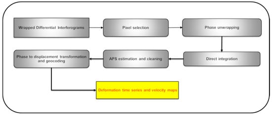
Figure 1.
Direct integration (DI) approach.
- (i)
- Pixel selection and phase unwrapping: We select the points that have average coherence above a given threshold. The average coherence is the average of the coherences of the whole set of interferograms. Those points with coherence smaller than the selected threshold are removed before phase unwrapping. We usually select a low threshold to include the maximum number of points. Then, these selected pixels of all the N-1 interferograms undergo phase unwrapping, which is performed using the minimum cost flow (MCF) method described in [22].
- (ii)
- Direct integration of the phases: the accumulated phase over time is estimated for each point as follows:where is the accumulated phase at the acquisition time i, and is the interferometric phase between the images i and i − 1.
- (iii)
- Atmospheric phase screen (APS) filtering: In this step, the Butterworth filter (a low-pass filter) is used to remove the atmospheric contribution to the phases (very low spatial phase variation). A temporal filter is then applied to separate the APS signal from the temporally correlated components, usually associated with terrain deformations.
- (iv)
- Phase to displacement transformation and geocoding: The accumulated phase of each measured point is transformed into displacement as follows:where is the wavelength. The final step is the geocoding where the corresponding ground coordinates for each pixel are found. This approach is not supervised and does not provide quality estimators. As explained later in this document, this method is not robust against the so-called fading effects [42]. However, it provides quantitative measurements that can be helpful to decide to apply more reliable approaches.
2.2. PSIG Short Temporal Baseline Approach
The main objective of the PSIG chain is to extend the interferometric analysis to wider areas using a unique, redundant, and connected network of points. The main goal is to propose a method with the same reliability of the standard A-DInSAR approaches but significantly improving the sampling density and reducing the phase unwrapping error sources [26].
Here, we propose a slightly different PSIG approach by constraining the temporal baselines to a given threshold, the PSIG-STB approach. The inputs include a stack of N co-registered SAR images, the dispersion of amplitude or coherence images, and M wrapped interferograms, with M >> N. For each image, all the possible interferograms below a temporal baseline threshold are generated. The goal of the network is to ensure a good temporal sampling, while preserving a high interferometric coherence. For instance, in the cases discussed in this paper, we have used interferograms with temporal baselines lower than 30 days. The procedure is illustrated in Figure 2. The main steps are described here below:
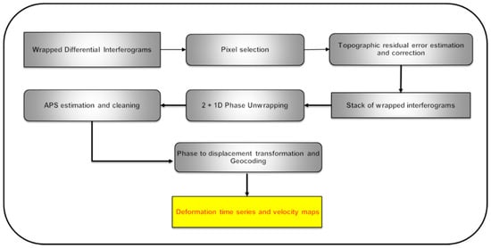
Figure 2.
Persistent scatterer interferometry geomatics short temporal baseline (PSIG-STB) approach.
- (i)
- Pixel selection: The first step is the pre-pixel selection. It is based on the dispersion of amplitude index [26]. The threshold might vary for different sites and the final value seeks a trade-off between sampling density and noise.
- (ii)
- Topographic error estimation and correction: In this step, the topographic error of the DEM used in the interferogram generation is estimated. The assumption is that the phase component related to the residual topographic error, the thermal phase component, and the phase noise are spatially uncorrelated. Given this assumption, the atmospheric component is the only phase component spatially correlated over stables areas. The approach used is described in [26] and is based in the maximization of the function:where is the gamma value, also called temporal coherence, N is the number of images, and N − 1 are the interferograms generated using consecutive images. S-1 means interferograms with temporal baselines of 6–12 days. This network allows for hypothesizing that the phase component caused by movement is almost negligible in most of the interferograms. is the i-th interferogram of our network, and is the function that estimates the corresponding phase in an interferogram with the same perpendicular baseline of and with a topographic error etop. The algorithm is based on brute force.
A range of potential topographic errors is tested, and the one that reaches the maximum γ is selected. The γ ranges between 0 and 1. The higher the value, the better the agreement between the topographic model and observations. Only those points with a γ higher than a given threshold are selected for the subsequent steps. The use of high coherent interferograms allows us to have a very dense network of points with relatively high γ. The estimated topographic error is removed from each interferogram for each selected point.
- (iii)
- 2 + 1D phase unwrapping: this step exploits a two-step phase unwrapping described in [26]. The first step consists in a spatial phase unwrapping. The algorithm used is based in the minimum cost flow method [22] and is performed for each interferogram of the network and only using the points selected in the previous step. The second step is carried out point wise and performs a temporal consistency check of the unwrapped interferograms. The approach consists of solving the following system for each point:
The system is solved by means of an iterative LS with outlier rejection. The key variable are the residuals ▁φ_Res, and the network redundancy and the number of interferograms that are directly tied to each image, i.e., the number of interferograms where a given image appears either as master or slave. The iterative process steps are:
- First LS estimation and computation of the residuals.
- Temporal removal of the highest absolute residual from the network (outlier candidate).
- New LS estimation.
- To check the outlier candidate new residual. If it becomes a multiple of 2π ± ε, the observation is corrected and reaccepted to the network. Otherwise, it is reaccepted only if the new residual is below a given threshold.
The process from (2) to (4) is repeated until there is not residual above a given threshold. The mean feature of the outlier rejection efficiency is given by the redundancy matrix R. It is well known that LS method is not robust. A given error might be spread out through the network according to the characteristics of the design (A) and the weight (P) matrix. To properly detect outliers (2π multiples in our case), it is necessary to analyze how the errors are distributed in the network. This information is contained in the redundancy matrix R [43]:
As it is observed, R is only related to A and P, i.e., it is independent of the observation vector. This matrix is used to correct the LS residuals using the redundancy of the corresponding observations:
where is the corrected i-th residual, and is the i-th diagonal element of R, which is called the local redundancy. Step 4 of the procedure is performed on the corrected residuals. With a proper network redundancy, the unwrapping errors are properly identified. However, it is worth noting that there is an intrinsic assumption that the majority of the interferograms connected to a given image are correctly unwrapped. The local redundancy is checked at each iteration: the algorithm checks the available local redundancy at each iteration. If the redundancy of a given outlier candidate is too low, it is not modified. That means that the algorithm only works over the redundant parts of the analyzed network. The weaker parts of the network must be checked off-line after the automatic analysis has concluded.
The particular aspect of this procedure is the network used using S-1 imagery. The high temporal sampling allows redundant networks to be produced with more than five interferograms per image with maximum temporal baselines of 30–60 days. Under these conditions, i.e., dense networks of points without topographic component and with low noise, the spatial phase unwrapping use to have reliable behavior, and the temporal consistency check provides its best performances. The final output of this step is, for each point, the temporal evolution of the phase, i.e., the time series.
After the 2 + 1D phase unwrapping, we perform the APS filtering in the same way as in the DI procedure, and we conclude with the estimation of the deformation velocity by using a robust linear regression for each displacement time series. In the present scenario, the PSIG-STB approach was developed as a different validation approach, when the DI approach revealed a peculiar systematic signal [42] in multi-looked 6-day interferograms, especially in large, high-humidity areas. If unattended, this particular signal can bias the deformation estimates of PS. The PSIG-STB approach proved itself a competent alternative in areas where the DI approach exhibited fading signals.
3. Results
In this section, we describe three case studies over the areas shown in Figure 3, where the proposed methodologies are applied for the semi-automatic identification and pre-screening of the deformation processes. Firstly, we propose a successful case of application of the DI: a region located in the north of Chile, entailing two open pit mines. Secondly, we propose a less favorable case of DI but successful for PSIG-STB, the Hierro Island test site. Finally, we propose an example of Barcelona metropolitan area where the results of PSIG-STB have been used operatively to monitor different infrastructures.
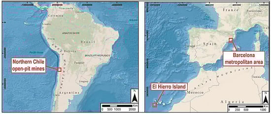
Figure 3.
Study areas.
3.1. North Chile Region
The underground mining of mineral and ore deposits is widespread across the world. One of the side effects of mineral extraction is the occurrence of ground movements. These movements might be caused by changes in the distribution of load on the hard ground beneath or by water extraction from the aquifers.
The monitoring of ground displacements is currently most often carried out with the use of traditional surveying methods, mainly precise levelling. Due to limitations such as spatial restrictions and high costs posed by classical measurement methods, DInSAR has become a very effective solution for the observation of ground movements in mining areas.
This first test site is a positive case of application of the DI approach. It is an illustrative example to show how we can obtain fast and unsupervised accumulated displacement maps over wide regions to map potential active areas in remote and natural environments. It is applied along a river basin, located in the central north of Chile (longitude −77.33° and latitude −27.35°). Figure 4 shows the accumulated deformation along the period ranging from October 2014 to March 2019, in ascending orbit. The number of processed images and interferograms is 81 and 80, respectively.
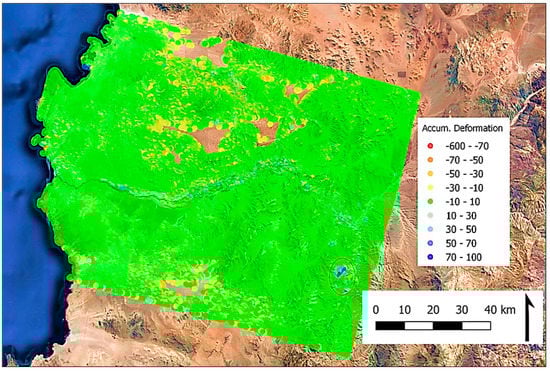
Figure 4.
Accumulated deformation at the Chile river basin during the period 2015–2020. The red ellipse bounds the area shown in Figure 5.
The total number of points is 2,374,445. The time of processing is around 370 min with an Intel Core I5-6600 CPU @ 3.30 GHz and 32 GB of RAM. The processing is performed pixel-wise without parallelization. Thus, the time could be reduced drastically. At a first glance, it is easy to observe the high coverage of the obtained results. The accumulated deformation map resulted in a standard deviation (σ) of 5 mm. We have used two times the σ value as a stability threshold (at 10 mm). With this threshold, 7% of the points are considered moving points.
Figure 5 shows an interesting area affected by displacements, with the corresponding deformation time series (Figure 6) of four selected points: one stable (P3) and three unstable (P1, P2, and P4). Movements towards the satellite are shown in blue (positive values), while movements away from the satellite are shown in red (negative values). In this case, the detected movements are caused by different mining activities. The displacements shown by P2 and P4 are related to slope instability areas along the open-pit slopes very common in open-pit mines [37]. A significant contribution of the topographic errors are discarded because there in these areas is not observed a correlation between perpendicular baselines series and time series. The maximum measured displacements are around −60 mm/year (P2 area) and −30 mm/year (P4 area). Although these numbers must be considered a very rough estimation, a proper analysis can provide an idea of the movement magnitudes. Another interesting movement is the upheaval of the tailing dam (P1 area), where by-products of the mining operations are stored and accumulated (Figure 5). Again, we discard topographic errors comparing time series evolution and perpendicular time series. The accumulated displacement raises in an average of 55 mm. All the time series displayed in Figure 6 show almost regular trends despite having a discontinuity in the time series (bounded by a rectangle, indicating the period where images were not available). However, because of this gap, the values of displacement can be underestimated due to phase unwrapping errors. The DI method does not have any quality estimator. It is worth noting that, despite these potential errors, the target of the analysis is fulfilled, since it provides enough information to detect active areas.
Figure 5.
Copper mining pits displaying deformation—example 1. The accumulated displacement time series of the points P1, P2, P3, P4, and P5 are shown in Figure 6.
Figure 6.
Deformation time series of north Chile open-pit mine—example 1 of points P1, P2, P3, P4, and P5 shown in Figure 5.
Figure 7 show another example of a different copper mine out of the same river basin shown in Figure 4. In this case, we used the DI approach to data acquired during a year (August 2018–July 2019), also in the ascending orbit. The area under study shows very high deformations, which is demonstrated with the time series of points P1, P2 (slopes) and P3, P4 (stacks) in Figure 8. The displacements ranging from −60 cm/year to 20 cm/year are mainly due to settlements of mining wastes in the stacks and slope instabilities of the mining pits, similar to the previous example. Most of the deformation points showed liner or bilinear trends in the time series. These points also displayed brief periods of stability. The results, in this case, show the ability of the proposed approach to properly detect active areas. Moreover, the approach can be used as a tool for supporting in situ measurement by providing information about the area of influence of the phenomena.
Figure 7.
Copper mining pits displaying deformation—example 2. The accumulated displacement time series of the points P1, P2, P3, and P4 are shown in Figure 8.
Figure 8.
Deformation time series of north Chile open-pit mine—example 2 of points P1, P2, P3, and P4 shown in Figure 7.
3.2. The Hierro Island
El Hierro is the south-westernmost island of the Canarias archipelago (Spain), located in the Atlantic Ocean off the coast of Africa. El Hierro Island is volcanic and sharply mountainous, hence it is a highly prone area to landslides and slope failures. Hence, the goal was to rapidly and semi-automatically generate a product to be easily exploited in the geohazard management by the Civil Protections Authorities and the Geological Surveys. The accumulated deformation map of El Hierro obtained with 2 × 10 multi-looked images using the DI approach is shown in Figure 9.
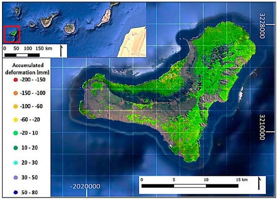
Figure 9.
Satellite image showing the location of El Hierro in the Canaryian archipelago (Spain) and accumulated deformation map estimated for El Hierro island using the DI approach. The sampling density achieved (approximately 400 PS/km2) can be inferred from this image.
The land cover is mainly volcanic rock fall, with sparse vegetation, thus assuring high coherent radar response. The area of the island is approximately 260 km2. The interferograms have good coherence, and the occasional loss of coherence mainly affected the vegetated areas in the center of the island. A stack of 74 S-1 images acquired in ascending orbit and 73 6-day interferograms were processed. The period of observations covers from 26 May 2017 to 2 July 2018. The points with mean coherence higher than 0.25 were used for the DI approach. The sampling density achieved in first instance was not deemed enough, and as a measure to improve the density of points, a spatial averaging within homogeneous coherent pixels of single look images were performed to form multi-looked observations. Most of the S-1 A-DInSAR processing approaches makes use of multi-looked images to reduce noise, but this averaging seems to be introducing a variant systematic signal, which shows no characteristics of stochastic noise, among the multi-looked interferograms, mimicking deformation signal patterns (Figure 10). This signal, which in this case is present in highly coherent points, is not filtered out during pixel selection and can be wrongly interpreted as deformation patterns, especially when prior knowledge about the area under observation is unavailable. The complex geophysical characteristics of the island, such as the coasts and the presence of high cliffs, has significant influence in the signals. This signal is named “fading signals” because of the reason that the signal perishes with the increment in temporal baseline [42].
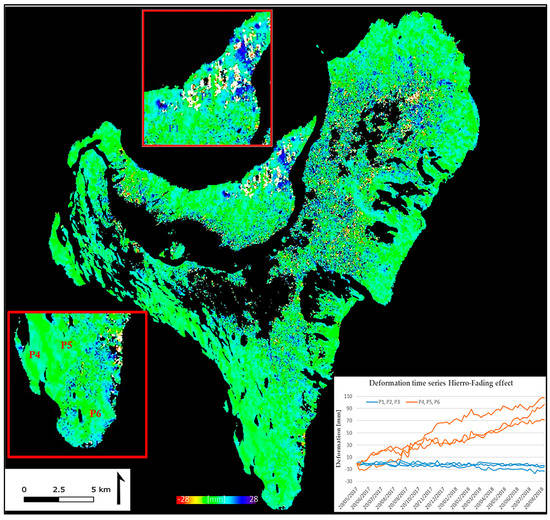
Figure 10.
Accumulated displacement map of El Hierro island and examples of time series obtained with the DI approach. The time series of two sets of points P1, P2, P3 and P4, P5, P6 located in the seemingly unstable and stable areas of the island, respectively, are shown to demonstrate fading effects.
Figure 10 shows the same result of Figure 9 but in SAR geometry. The goal of this figure is to emphasize some peculiar deformation areas and to better show the level of noise of the results. The figure displays the time series of two points in two different parts of the island. The first point is located in the north of the island. Even though it does not display a huge linear trend as point 2, it still shows a slight shift away from the satellite that can be wrongly interpreted as deformation. The second point displays a linear systematic trend towards the satellite starting from 0 to 16 mm in a period of one year, which can be characterized as upheaval under usual deformation analysis.
Since ground validation of these deformations were difficult to undertake, and the area is of highly complex physical phenomena, it was practically easier to adopt a new method, which can omit this kind of points showing such deformation patterns, where in fact, we do not know if these deformations are actually happening.
Figure 11 shows the results obtained with (A) the DI, (B) the PSIG-STB, and (C) the PSIG approaches, respectively. Many of such highly coherent “problematic” points are filtered out in the PSIG-STB method. Almost all fading effects were filtered or not selected as good points. It can be seen that most of the points in (B) are showing an absolute deformation velocity below 1 mm/yr. The corresponding time series should ideally contain only a negligible deformation. Figure 12 shows one such point in the southern part of the island (P1 in Figure 11), which had shown fading effects, while using only the multi-looked 6-day interferograms in the DI approach. This unaccountable behavior has been corrected using the PSIG-STB approach. This approach also has the same advantages of DI, i.e., easy to implement, but also provides robust results. However, the point density is sensibly lower. The accumulated deformation map resulted in a standard deviation (σ) of 0.95 mm, proving that most parts of the island displayed stable behavior in the PSIG-STB approach. Only the time series corresponding to 8657 points out of 57,821 points included in the dataset (i.e., the 15% of the points) have a total standard deviation higher than 1.9 mm. These statistics were considered satisfactory in the considered deformation monitoring.
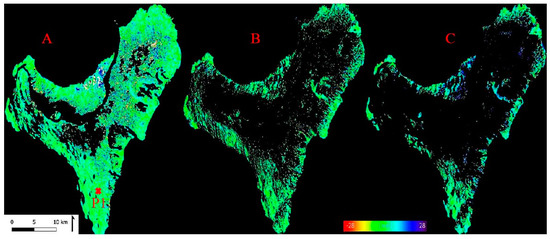
Figure 11.
Accumulated deformation map of El Hierro island (Spain) estimated with multi-looked interferograms for a period of one year using (A) the DI approach, (B) the PSIG-STB approach, and (C) the standard PSIG approach.
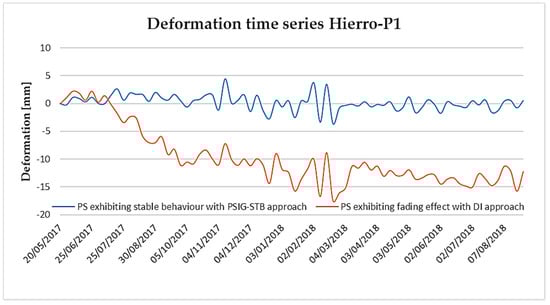
Figure 12.
Example of fading effect exhibited by point P1 in Figure 11 estimated using the DI approach in comparison with the same point exhibiting stable behavior estimated using the PSIG-STB approach.
To assess the performance of PSIG-STB approach, we also processed the standard PSIG chain described in [26]. The comparison between the accumulated deformation estimated using the standard PSIG approach and the PSIG-STB approach is also provided in Figure 11. The main advantages of the PSIG-STB approach over the standard PSIG approach is the reduction in phase unwrapping errors and jumps and an increase of 6% of the point density, i.e., 57,821 points using the PSIG-STB and 54,545 using the standard PSIG. This is not a minor increase considering that the area is almost natural. The PSIG-STB approach is faster than the standard PSIG approach, which efficiently and effectively filters out all the problematic points, showing fading effects. Especially, in this case where pixel selection with high coherence or dispersion of amplitude (DA) did not eliminate the points with strange trends, because the island has a high radar response. Finally, it is worth noting that the PSIG approach shows an uplift area in the north east of the island. To the authors’ knowledge, there should not be this type of activity during the monitored period [44]. Thus, we interpret that it could be related to phase unwrapping errors due to atmosphere. It is clearly seen that these artifacts are not present in the PSIG-STB results.
3.3. Barcelona Metropolitan Area
The PSIG-STB procedure has been applied to the metropolitan area of Barcelona, Catalonia, Spain. Different types of geohazards such as urban settlement, mining subsidence, and landslides have been identified in this study area. The inherently short-lived but physically present “fading signals” were attributed as an outcome of multi-looked SAR images in [40]. However, in the study area of Catalonia, these signals were again present under the DI approach. Note that the two conventional product estimates of DInSAR, the surface displacement time series and displacement velocity are both compromised in the presence of these fading signals. Hence, we considered this study area was suitable to perform an additional, complementary deformation monitoring analysis using PSIG-STB. In this case study, we limit our analysis to the efficiency in detection of PS and displacement time series, as it is usually done in urban applications, using PSIG-STB.
The study area lies in the region of Catalonia, which is covered by a single S-1 frame. The analyzed dataset includes 245 SLC S-1 images, which cover the period from 6 March 2015 to 26 May 2020. The interferograms were generated at full resolution using all possible image combinations, with a limit of 60 days. Even though the decorrelation was mainly due to vegetation coverage and topography, a good compromise had to be made between the noisy phase and the spatial coverage of PSs. Points with dispersion of amplitude lower than 0.4 were selected for the processing.
Figure 13 shows the estimated accumulated displacement map for the processed area (A) and for a zone of the Barcelona harbor (B). In Figure 13A, we observe several displacement areas that correspond to different movement phenomena such as mining activities, intense water extraction, or urban construction as well as heavy surface loads or landslides. Figure 13B shows a magnified portion with the Barcelona port and El Prat airport. Port dikes show values of more than 10 cm of accumulated displacement from January 2017 to January 2019.
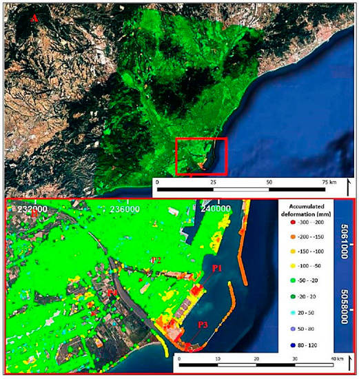
Figure 13.
Accumulated deformation map of Barcelona metropolitan area (A) with a zoom of the Barcelona port dikes with more than 10 cm of accumulated displacement from January 2017 to January 2019 (B). The displacement time series of the points P1, P2, P3, P4 are shown in Figure 14.
Figure 14 shows four examples of time series of point P1, P2, P3, and P4 indicated in Figure 13, where different types of behaviors can be identified. In a relatively small area, there are deformations corresponding to an uplift (P4), probably related to underground water recovery. Some of the uplift detected in areas along the shores of the Llobregat River is mainly caused by sedimentation. The displacement in the whole frame ranged from −300 mm/year to 150 mm/year. Then, there are PSs that are moving away from the satellite revealing a significant amount of sinking or subsidence, such as the points in the port and some structures in the urban area (P1 and P3): settlements in the dyke (P3) or in the harbor (P1). Then, there are stable points where all the observations are consistent, with less or no outlier candidates (e.g., P2), which helps us to assess the quality of the deformation time series.
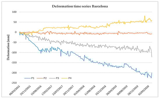
Figure 14.
Accumulated deformation time series for a period of 5 years of points P1, P2, P3, and P4 in Figure 13 using the PSIG-STB approach with full-resolution SLC images.
4. Discussion
With the implementation of the fully automatic approaches in three different areas, characterized by substantially different physical, geographical, and meteorological conditions, it can be inferred that an unsupervised identification and pre-screening of the deformational processes is possible. The results of copper mines (Chile study case) demonstrate the capability of the DI approach to discern active areas and to deliver high-quality deformation maps to aid in situ monitoring. In this area of dry physiography, the DI approach revealed very high deformations. So even with phase unwrapping errors, it gave enough information to end-users to conclude whether a comprehensive analysis of the active areas is necessary. Future investigations should test methods to better understand the nature and mitigate the effects of the fading effect in multi-looked interferograms (as shown for El Hierro) and to find ways to detect points potentially affected by unwrapping errors.
In a general context, the DI approach can be considered non-robust and very sensible to phase unwrapping sources. However, its performances with Sentinel-1 data are good enough to make it a useful tool for pre-screening. The Sentinel-1 tube assures perpendicular baselines lower than 300 m. This means that in the worst situation, two times the height accuracy of the SRTM (20 m) would correspond approximately with the 30% of the phase cycle, i.e., far from a phase ambiguity. This combined with multi-looking, which usually smooths topographic errors, mitigates the topographic.
Errors influence the phase unwrapping. A good example of this is provided by the open pit mine area shown in the previous section. In these areas, the topographic errors are an important source of error. The spatial correlation of the active areas and the decorrelation with the perpendicular baselines help to discard the influence of topography in such areas.
Once an area is mapped as a potential displacement area, a more robust analysis is required in order to understand its spatial and temporal behavior. The PSIG-STB approach provides this robustness, keeping an acceptable high spatial sampling. This approach has been demonstrated to be a method able to be used in both urban and natural environments, showing robust results. However, compared to the DI, it shows a significant decrease in the sampling density, which can result in the loss of key information. Thus, a systematic approach to deal with wide areas can be to use the DI to rapidly detect those areas potentially affected by displacement and then apply the STB-PSIG on the detected moving areas.
Some of the characteristic spikes and dips in the deformation time series correspond to phase unwrapping errors when the jump between two consecutive dates is equal to 2π or multiples of 2π. These errors are very common in A-DInSAR analysis and tolerable, since many times, they can be identified and rectified with point-by-point analysis. Although an overall improvement was visible with phase unwrapping, in the PSIG-STB approach, the main advantage of both the methods as mentioned before has to be the promptitude, which is quite essential when it comes to having a pilot study of the area of interest, with a self-driven flow chain. If we consider the processing time, the standard PSIG chain remains the reference technique. After all, it has to be noted that the time series of the PSs depicted in the paper is the result of two automated approaches; it can definitely be improved with careful and skilled interpretation and rectification.
While dealing with the fading effects in further studies, it is debatable whether it is possible to insert a form of “intelligent filter” in the downstream of the processing chain that can distinguish the reliable time series from the artificially created ones. Unfortunately, this work supports the inference that this distinction is not feasible. Because our results show that the artificially created fading effects also exhibit linear or bilinear trends similar to a deformation time series. Thus, a pixel selector upstream of the processing chain that helps to identify the good points offers the advantage of not interpreting artificial trends as real ones.
Finally, it is worth mentioning that the forthcoming constellations such as Capella Space or Ice Eye will be able to provide shorter revisit times. Therefore, with such a short revisit time, arises a need for near real-time processing, to fully exploit the data available soon. In such a scenario, the proposed approaches will be really useful as automated tools to perform a preliminary study.
5. Conclusions
Two complementary approaches to process wide areas with Sentinel-1 data have been presented in this document: the DI and the PSIG-STB approaches. Both approaches provide fast and straightforward solutions to analyze deformations affecting large areas.
The main characteristics and performances of the proposed procedures have been illustrated in the results obtained from three different cases of study. The main advantages and drawbacks have been pointed out and discussed. The DI approach provides a light way for fast analysis of large areas, assuring good point density but has a strong dependence on the operator data analysis skills. The PSIG–STB approach provides a robust method able to assess the reliability of the active areas detected by the DI but also very useful to be used instead of standard A-DInSAR approaches. It provides very nice performances compared to a classical PS chain such as the PSIG approach by improving both the point density and the robustness against phase unwrapping errors. For further filtering of points, the generation of a quality index for each image of a given deformation time series can be carried out [11].
In this paper, we also pointed out the presence of a peculiar systematic signal in InSAR. The results show that the appearance of such fading signals that can lead to wrong interpretation of false ground movements. The analysis of such fading signals serves as an example to show that, for an effective calibration, we need to perform comprehensive research on various possible physical sources of inconsistencies and design case-specific models to explain the interferometric phase of each source. Another solution is to derive a technique to validate or discard the fading signals. Generally, the PSI validation activities are based on the comparison of deformation velocities and time series with independent estimations of the same quantities acquired by sources of better quality, e.g., levelling or GPS measurements. In any case, for the fading effects, further studies on various test sites are inevitable.
As mentioned before, the main advantages of the proposed methods are the promptness, convenience, and the possibility of an automatic generation of deformation maps and time series to reveal displacement phenomena for wide areas and to fully exploit the detection ability of InSAR based on S-1 datasets [13]. In addition, improvements in the time series as well as in the density of points are observed for all the datasets using the DI and PSIG-STB methods in comparison to the traditional PSIG chain.
Author Contributions
V.K. and O.M. conceptualized and consolidated the draft; O.M., V.K., and Z.Q. developed and implemented the methodology; R.P., B.C., and A.B. developed the software; M.C.-G. and Q.G. processed and validated the PS data; J.L.-V. and C.R.-C. analyzed and reviewed the results. J.A.G. supervised the project. All the authors contributed to performing the experiments; all the authors contributed to writing the paper. All authors have read and agreed to the published version of the manuscript.
Funding
This work has been partially funded by AGAUR, Generalitat de Catalunya, through a grant for the recruitment of early-stage research staff (Ref: FI_B 00741) and through the Consolidated Research Group RSE, “Remote Sensing” (Ref: 2017-SGR-00729). It has been also partially funded by the Spanish Ministry of Economy and Competitiveness through the DEMOS project “Deformation monitoring using Sentinel-1 data” (Ref: CGL2017-83704-P) and by AGAUR.
Institutional Review Board Statement
Not applicable.
Informed Consent Statement
Not applicable.
Data Availability Statement
Data are available at CTTC.
Acknowledgments
QGIS.org, 2020. QGIS Geographic Information System. QGIS Association. http://www.qgis.org accessed on 1 February 2021.
Conflicts of Interest
The authors declare no conflict of interest.
References
- Zebker, H.A.; Rosen, P.A.; Hensley, S. Atmospheric effects in interferometric synthetic aperture radar surface deformation and topographic maps. J. Geophys. Res. Space Phys. 1997, 102, 7547–7563. [Google Scholar] [CrossRef]
- Amelung, F.; Galloway, D.L.; Bell, J.W.; Zebker, H.A.; Laczniak, R.J. Sensing the ups and downs of Las Vegas: InSAR reveals structural control of land subsidence and aquifer-system deformation. Geology 1999, 27, 483–486. [Google Scholar] [CrossRef]
- Gao, Q.; Zribi, M.; Escorihuela, M.J.; Baghdadi, N. Synergetic use of Sentinel-1 and Sentinel-2 data for soil moisture mapping at 100 m resolution. Sensors 2017, 17, 1966. [Google Scholar] [CrossRef]
- Madsen, S.; Zebker, H.; Martin, J. Topographic mapping using radar interferometry: Processing techniques. IEEE Trans. Geosci. Remote Sens. 1993, 31, 246–256. [Google Scholar] [CrossRef]
- Raspini, F.; Bianchini, S.; Ciampalini, A.; Del Soldato, M.; Montalti, R.; Solari, L.; Tofani, V.; Casagli, N. Persistent scatterers continuous streaming for landslide monitoring and mapping: The case of the Tuscany region (Italy). Landslides 2019, 16, 2033–2044. [Google Scholar] [CrossRef]
- Delouis, B.; Nocquet, J.-M.; Vallée, M. Slip distribution of the February 27, 2010 Mw = 8.8 Maule Earthquake, central Chile, from static and high-rate GPS, InSAR, and broadband teleseismic data. Geophys. Res. Lett. 2010, 37. [Google Scholar] [CrossRef]
- Béjar-Pizarro, M.; Álvarez Gómez, J.A.; Staller, A.; Luna, M.P.; Pérez-López, R.; Monserrat, O.; Khunga, K.; Lima, A.; Galve, J.P.; Martinez Diaz, J.J.; et al. InSAR-based mapping to support decision-making after an earthquake. Remote Sens. 2018, 10, 899. [Google Scholar] [CrossRef]
- Solari, L.; Del Soldato, M.; Raspini, F.; Barra, A.; Bianchini, S.; Confuorto, P.; Casagli, N.; Crosetto, M. Review of satellite interferometry for landslide detection in Italy. Remote Sens. 2020, 12, 1351. [Google Scholar] [CrossRef]
- Wegmüller, U.; Walter, D.; Spreckels, V.; Werner, C.L. Nonuniform ground motion monitoring with TerraSAR-X persistent scatterer interferometry. IEEE Trans. Geosci. Remote Sens. 2009, 48, 895–904. [Google Scholar] [CrossRef]
- Yu, B.; Liu, G.; Li, Z.; Zhang, R.; Jia, H.; Wang, X.; Cai, G. Subsidence detection by TerraSAR-X interferometry on a network of natural persistent scatterers and artificial corner reflectors. Comput. Geosci. 2013, 58, 126–136. [Google Scholar] [CrossRef]
- Crosetto, M.; Monserrat, O.; Cuevas-González, M.; Devanthéry, N.; Crippa, B. Persistent scatterer interferometry: A review. ISPRS J. Photogramm. Remote Sens. 2016, 115, 78–89. [Google Scholar] [CrossRef]
- Aslan, G.; Foumelis, M.; Raucoules, D.; De Michele, M.; Bernardie, S.; Cakir, Z. Landslide mapping and monitoring using Persistent Scatterer Interferometry (PSI) technique in the French Alps. Remote Sens. 2020, 12, 1305. [Google Scholar] [CrossRef]
- Reyes-Carmona, C.; Barra, A.; Galve, J.P.; Monserrat, O.; Pérez-Peña, J.V.; Mateos, R.M.; Notti, D.; Ruano, P.; Millares, A.; López-Vinielles, J.; et al. Sentinel-1 DInSAR for monitoring active landslides in critical infrastructures: The case of the Rules Reservoir (Southern Spain). Remote Sens. 2020, 12, 809. [Google Scholar] [CrossRef]
- Costantini, M.; Ferretti, A.; Minati, F.; Falco, S.; Trillo, F.; Colombo, D.; Novali, F.; Malvarosa, F.; Mammone, C.; Vecchioli, F.; et al. Analysis of surface deformations over the whole Italian territory by interferometric processing of ERS, Envisat and COSMO-SkyMed radar data. Remote Sens. Environ. 2017, 202, 250–275. [Google Scholar] [CrossRef]
- Solari, L.; Crosetto, M.; Balasis-Levinsen, J.; Casagli, N.; Frei, M.; Moldestad, D.A.; Oyen, A. The European Ground Motion Service: A continental scale map of ground deformation. In Proceedings of the EGU General Assembly Conference Abstracts, Online, 4–8 May 2020; p. 3148. [Google Scholar]
- Solari, L.; Bianchini, S.; Franceschini, R.; Barra, A.; Monserrat, O.; Thuegaz, P.; Bertolo, D.; Crossetto, M.; Catani, F. Satellite interferometric data for landslide intensity evaluation in mountainous regions. Int. J. Appl. Earth Obs. Geoinf. 2020, 87, 102028. [Google Scholar] [CrossRef]
- Frattini, P.; Crosta, G.B.; Rossini, M.; Allievi, J. Activity and kinematic behaviour of deep-seated landslides from PS-InSAR displacement rate measurements. Landslides 2018, 15, 1053–1070. [Google Scholar] [CrossRef]
- Barra, A.; Solari, L.; Béjar-Pizarro, M.; Monserrat, O.; Bianchini, S.; Herrera, G.; Crosetto, M.; Sarro, R.; González-Alonso, E.; Mateos, R.M.; et al. A methodology to detect and update active deformation areas based on Sentinel-1 SAR images. Remote Sens. 2017, 9, 1002. [Google Scholar] [CrossRef]
- Intrieri, E.; Raspini, F.; Fumagalli, A.; Lu, P.; Del Conte, S.; Farina, P.; Allievi, J.; Ferretti, A.; Casagli, N. The Maoxian landslide as seen from space: Detecting precursors of failure with Sentinel-1 data. Landslides 2018, 15, 123–133. [Google Scholar] [CrossRef]
- Hanssen, R.F. Radar Interferometry: Data Interpretation and Error Analysis; Springer Science and Business Media LLC: Amsterdam, The Netherlands, 2001; Volume 2. [Google Scholar]
- Monserrat, O.; Crosetto, M.; Cuevas, M.; Crippa, B. The thermal expansion component of persistent scatterer interferometry observations. IEEE Geosci. Remote Sens. Lett. 2011, 8, 864–868. [Google Scholar] [CrossRef]
- Costantini, M. A novel phase unwrapping method based on network programming. IEEE Trans. Geosci. Remote Sens. 1998, 36, 813–821. [Google Scholar] [CrossRef]
- Pepe, A.; Euillades, L.D.; Manunta, M.; Lanari, R. New advances of the extended minimum cost flow phase unwrapping algorithm for SBAS-DInSAR analysis at full spatial resolution. IEEE Trans. Geosci. Remote Sens. 2011, 49, 4062–4079. [Google Scholar] [CrossRef]
- Yang, Y.; Pepe, A.; Manzo, M.; Casu, F.; Lanari, R. A region-growing technique to improve multi-temporal DInSAR interferogram phase unwrapping performance. Remote Sens. Lett. 2013, 4, 988–997. [Google Scholar] [CrossRef]
- Yu, H.; Lee, H.; Yuan, T.; Cao, N. A novel method for deformation estimation based on multibaseline InSAR phase unwrapping. IEEE Trans. Geosci. Remote Sens. 2018, 56, 5231–5243. [Google Scholar] [CrossRef]
- Devanthéry, N.; Crosetto, M.; Monserrat, O.; Cuevas-González, M.; Crippa, B. An approach to persistent scatterer interferometry. Remote Sens. 2014, 6, 6662–6679. [Google Scholar] [CrossRef]
- Shamshiri, R.; Motagh, M.; Nahavandchi, H.; Haghighi, M.H.; Hoseini, M. Improving tropospheric corrections on large-scale Sentinel-1 interferograms using a machine learning approach for integration with GNSS-derived zenith total delay (ZTD). Remote Sens. Environ. 2020, 239, 111608. [Google Scholar] [CrossRef]
- Huang, Q.; Crosetto, M.; Monserrat, O.; Crippa, B. Displacement monitoring and modelling of a high-speed railway bridge using C-band Sentinel-1 data. ISPRS J. Photogramm. Remote Sens. 2017, 128, 204–211. [Google Scholar] [CrossRef]
- Crosetto, M.; Solari, L.; Mróz, M.; Balasis-Levinsen, J.; Casagli, N.; Frei, M.; Oyen, A.; Moldestad, D.A.; Bateson, L.; Guerrieri, L.; et al. The evolution of wide-area DInSAR: From regional and national services to the European Ground Motion Service. Remote Sens. 2020, 12, 2043. [Google Scholar] [CrossRef]
- Barra, A.; Monserrat, O.; Mazzanti, P.; Esposito, C.; Crosetto, M.; Mugnozza, G.S. First insights on the potential of Sentinel-1 for landslides detection. Geomat. Nat. Hazards Risk 2016, 7, 1874–1883. [Google Scholar] [CrossRef]
- Bru, G.; González, P.J.; Mateos, R.M.; Roldán, F.J.; Herrera, G.; Béjar-Pizarro, M.; Fernández, J. A-DInSAR monitoring of landslide and subsidence activity: A case of urban damage in Arcos de la Frontera, Spain. Remote Sens. 2017, 9, 787. [Google Scholar] [CrossRef]
- González, P.J.; Bagnardi, M.; Hooper, A.J.; Larsen, Y.; Marinkovic, P.; Samsonov, S.V.; Wright, T.J. The 2014-2015 eruption of Fogo volcano: Geodetic modeling of Sentinel-1 TOPS interferometry. Geophys. Res. Lett. 2015, 42, 9239–9246. [Google Scholar] [CrossRef]
- Albino, F.; Biggs, J.; Yu, C.; Li, Z. Automated methods for detecting volcanic deformation using Sentinel-1 InSAR time series illustrated by the 2017–2018 unrest at Agung, Indonesia. J. Geophys. Res. Solid Earth 2020, 125, e2019JB017908. [Google Scholar] [CrossRef]
- Sowter, A.; Amat, M.B.C.; Cigna, F.; Marsh, S.; Athab, A.; Alshammari, L. Mexico City land subsidence in 2014–2015 with Sentinel-1 IW TOPS: Results using the Intermittent SBAS (ISBAS) technique. Int. J. Appl. Earth Obs. Geoinf. 2016, 52, 230–242. [Google Scholar] [CrossRef]
- Delgado Blasco, J.M.; Foumelis, M.; Stewart, C.; Hooper, A. Measuring urban subsidence in the Rome metropolitan area (Italy) with Sentinel-1 snap-stamps persistent scatterer interferometry. Remote Sens. 2019, 11, 129. [Google Scholar] [CrossRef]
- Bakon, M.; Czikhardt, R.; Papco, J.; Barlak, J.; Rovnak, M.; Adamisin, P.; Perissin, D. remotIO: A Sentinel-1 multi-temporal InSAR infrastructure monitoring service with automatic updates and data mining capabilities. Remote Sens. 2020, 12, 1892. [Google Scholar] [CrossRef]
- López-Vinielles, J.; Ezquerro, P.; Fernández-Merodo, J.A.; Béjar-Pizarro, M.; Monserrat, O.; Barra, A.; Blanco, P.; García-Robles, J.; Filatov, A.; García-Davalillo, J.C.; et al. Remote analysis of an open-pit slope failure: Las Cruces case study, Spain. Landslides 2020, 17, 2173–2188. [Google Scholar] [CrossRef]
- Zinno, I.; Bonano, M.; Buonanno, S.; Casu, F.; De Luca, C.; Manunta, M.; Manzo, M.; Lanari, R. National scale surface deformation time series generation through advanced DInSAR processing of Sentinel-1 data within a cloud computing environment. IEEE Trans. Big Data 2018, 6, 558–571. [Google Scholar] [CrossRef]
- Tomás, R.; Pagán, J.I.; Navarro, J.A.; Cano, M.; Pastor, J.L.; Riquelme, A.; Cuevas-González, M.; Crosetto, M.; Barra, A.; Monserrat, O.; et al. Semi-automatic identification and pre-screening of geological–geotechnical deformational processes using persistent scatterer interferometry datasets. Remote Sens. 2019, 11, 1675. [Google Scholar] [CrossRef]
- Lanari, R.; Bonano, M.; Casu, F.; De Luca, C.; Manunta, M.; Manzo, M.; Onorato, G.; Zinno, I. Automatic generation of Sentinel-1 continental scale DInSAR deformation time series through an extended P-SBAS processing pipeline in a cloud computing environment. Remote Sens. 2020, 12, 2961. [Google Scholar] [CrossRef]
- Galve, J.P.; Pérez-Peña, J.V.; Azañón, J.M.; Closson, D.; Calò, F.; Reyes-Carmona, C.; Jabaloy, A.; Ruano, P.; Mateos, R.M.; Notti, D.; et al. Evaluation of the SBAS InSAR service of the European Space Agency’s Geohazard Exploitation Platform (GEP). Remote Sens. 2017, 9, 1291. [Google Scholar] [CrossRef]
- Ansari, H.; De Zan, F.; Parizzi, A. Study of systematic bias in measuring surface deformation with SAR interferometry. IEEE Trans. Geosci. Remote Sens. 2021, 59, 1285–1301. [Google Scholar] [CrossRef]
- Förstner, W. Reliability, gross error detection and self-calibration. Int. Arch. Photogramm. Remote Sens. 1986, 26, 1–34. [Google Scholar]
- Béjar-Pizarro, M.; Herrera, G.; Sarro, R.; Mateos, R.M.; Barra, A.; González-Alonso, E.; Fernández, A.; Ligüerzana, S.; Garcia-Cañada, L.; Navarro, J. U-Geohaz D3.8 Deliverable-VEW Validation Report. Project U-Geohaz, Grant Agreement No. 783169. 2019. Available online: https://u-geohaz.cttc.es/download/deliverables (accessed on 1 February 2021).


Publisher’s Note: MDPI stays neutral with regard to jurisdictional claims in published maps and institutional affiliations. |
© 2021 by the authors. Licensee MDPI, Basel, Switzerland. This article is an open access article distributed under the terms and conditions of the Creative Commons Attribution (CC BY) license (http://creativecommons.org/licenses/by/4.0/).