A ROTI-Aided Equatorial Plasma Bubbles Detection Method

Abstract

In this study, we present a Rate of Total Electron Content Index (ROTI)-aided equatorial plasma bubbles (EPBs) detection method based on a Global Navigation Satellite System (GNSS) ionospheric Total Electron Content (TEC). This technique seeks the EPBs occurrence time according to the ROTI values and then extracts the detrended ionospheric TEC series, which include EPBs signals using a low-order, partial polynomial fitting strategy. The EPBs over the Hong Kong area during the year of 2014 were detected using this technique. The results show that the temporal distribution and occurrence of EPBs over the Hong Kong area are consistent with that of previous reports, and most of the TEC depletion error is smaller than 1.5 TECU (average is 0.63 TECU), suggesting that the detection method is feasible and highly accurate. Furthermore, this technique can extract the TEC depletion series more effectively, especially for those with a long duration, compared to previous method.

1. Introduction

Equatorial plasma bubbles (EPBs) are very frequent ionospheric events associated with the depletion in plasma density, which are widely believed to be generated by the Rayleigh–Taylor (R-T) instability in the F-layer [1,2]. The EPBs can cause the scintillations and huge ionospheric gradients of radio signals, leading to severe effects on navigation and communication systems [3]. As a result, the study on climatology and the forecasting of EPBs has remained an open question among the scientific community during the last two decades [4,5,6,7,8,9,10,11,12,13,14,15,16]. Many measurements, such as in situ satellite data [4,5], ionosonde [6], and airglow imaging [9,16] are applied to investigate the EPBs characteristics. In recent years, the Global Navigation Satellite System (GNSS) ionospheric Total Electron Content (TEC) has been an important tool for the study of EPBs due to its high spatial-temporal resolution [10,11,12,13,14,15].

To study the EPBs using GNSS TEC data, the first step is to extract the EPBs signals in the TEC series. One common method is using a polynomial fitting with a specific window length to fit the TEC series; then the detrended TEC series that might include EPBs signals are obtained by subtracting the fitted TEC series from the observed TEC series [11,12,13,14,15]. However, the detrended TEC series achieved by this method not only contain depletion but also enhancement, which is similar to the feature of the Medium-Scale Travelling Ionospheric Disturbances (MSTIDs). This exerts an adverse effect on distinguishing EPBs and MSTIDs. Magdaleno et al. [17] presented an Ionospheric Bubble Seeker (IBS) method to detect the EPBs. The IBS method applies the TEC variation and its variance to acquire the initial and end times of the EPBs; then, a linear fitting strategy is used to calculate the background TEC values during the period of EPBs. This method can obtain a good profile of the EPBs compared to the common method. However, the assumption that the profile of the background TEC is a straight line during the period of EPBs is inaccurate, especially for a long duration.

High-precision EPBs signals can help to understand the fine characteristics of EPBs and evaluate their effect on GNSS positioning accurately. To further improve the accuracy of the extracted EPBs signals, in this study, we attempted to employ the so-called Rate of TEC Index (ROTI) to seek the occurrence times of the EPBs and then use the low-order, polynomial fitting to calculate the background TEC values during the period of EPBs. In the following sections, we present the ROTI-aided EPBs detection method in detail and test it using GNSS data in Hong Kong.

2. Materials and Methods

2.1. Data

GNSS observations are the main data employed in this study. We downloaded the 30s-sampling GNSS observation files of station HKKT (receiver type is LEICA GRX1200+GNSS) in 2014 from the public website of Hong Kong’s satellite reference network [18].

2.2. Methods

The previous IBS method applied the variance of TEC variation to acquire the initial and end times of the EPBs [17]. According to the definition, the ROTI could be seen as the square root of the variance of TEC variation [19]. However, ROTI values are more widely used in monitoring ionospheric irregularities [11,20,21]. So, the “by-product” of the method in this study, namely the ROTI, is also meaningful.

The definition of ROTI is the standard deviation of the Rate of TEC (ROT) [19]. ROT at epoch $t_i$ can be computed using the following equation:

$$ROT\left(i\right)=\frac{1}{M{\left({\theta }_i\right)}^2}\frac{TEC\left(i\right)-TEC\left(i-1\right)}{t_i-t_{i-1}}$$

(1)

where $M\left(\theta \right)$ is the slant factor depending on satellite elevation ($\theta$) suggested by Sanz et al. [22]. Ionospheric TEC time series can be computed using the GNSS dual-frequency, geometry-free, combined carrier phase observations for each pair of satellite and receiver [23]. The ROTI over 5 min intervals of ROT data can be calculated as follows:

$$ROTI=\sqrt{\langle {ROT}^2\rangle -{\langle ROT\rangle }^2}$$

(2)

where the notation $\langle ·\rangle$ is the averaging operation. The unit of ROT and ROTI is TECU per min, where TECU is the unit of TEC (1 TECU = 10¹⁶/m²).

The ROTI series are then employed to seek the occurrence time of EPBs. Two thresholds, namely “up threshold” and “down threshold”, are adopted. For a period of TEC series $\left(T_1, T_2\right)$, if the ROTI values are larger than the down threshold and the maximum values are larger than the up threshold, then this period could have an EPB event. Then, we use the low-order polynomial (third order in this case) to fit the TEC data during $\left(T_1-7.5 \min , T_1\right)$ and $\left(T_2, T_2+7.5 \min \right)$. That is to say, the TEC data during the event $\left(T_1, T_2\right)$ are not used (see Figure 1). We call this strategy the partial fitting, as opposed to the general fitting method. Lastly, the detrended ionospheric TEC series, including possible EPB signals, are extracted by subtracting the fitted TEC series from the observed TEC series. If the TEC depletion maximum (called “depth”) and duration of the EPB candidate meet the defined thresholds then it can be confirmed as an EPB event or vice versa.

Table 1. Parameters of the ROTI-aided EPBs detection method.

Parameter	Value
Up ROTI	0.2 TECU/min
Down ROTI	0.04 TECU/min
Minimum depth	4 TECU
Minimum duration	10 min

lists the corresponding parameters of the EPBs detection method in this study. The minimums of depth and duration are set to 4 TECU and 10 min, respectively. According to the experimental results, the value of up ROTI could be set to 0.1–0.3 TECU/min (0.2 TECU/min here). The value of down ROTI is very important as it is related to the duration. Figure 2 presents the percent distribution of the ROTI values calculated for station HKKT during 2014. Considering that EPB generally occurs at night, only ROTI values from 6:00–18:00 LT are counted. As shown in Figure 2, the vast majority of the ROTI values are smaller than 0.04 TECU/min. Here, the value of down ROTI is set to 0.04 TECU/min. Furthermore, to distinguish from other events which lead not only to TEC depletion but also TEC enhancement (such as MSTIDs), the maximum of detrended TEC should be less than one-third of the depth.

3. Results

Figure 3 presents an example of the EPBs detection method in this study using station HKKT and satellite R04 on 28 February 2014. The blue line in panel (a) is the observed TEC series. The black line in panel (b) is the corresponding ROTI series calculated using Equations (1) and (2). The blue dotted line and red dotted line mark the thresholds of the up ROTI (0.2 TECU/min) and down ROTI (0.04 TECU/min), respectively. As shown in Figure 3b, the ROTI series during the period of $\left(T_1, T_2\right)$ meet the condition of the up and down thresholds (the maximum is 0.49 TECU/min). So, ionospheric irregularity during this period can be marked as an EPB candidate. The partially fitted TEC series, using a third-order polynomial, are also presented in panel (a) for comparison (green line). The red line in panel (c) is the detrended TEC series obtained by subtracting the fitted from the observed TEC series. As shown in Figure 3c, the depths (5.5 TECU) and duration (24 min) of the EPB candidates meet the defined thresholds. So, it can be confirmed that there is an EPB event in the ionosphere during the period of $\left(T_1, T_2\right)$.

Figure 4 presents the temporal distribution of the EPBs (top panel) and the percent distribution of EPBs occurrence (bottom panel) detected by the station HKKT, during 2014. As shown in Figure 4a, EPBs generally occur after 20:00 local time and are observed throughout the nighttime. As shown in Figure 4b, the occurrence of EPBs during the spring and autumn equinoxes is significantly greater than their occurrence during the summer and winter solstices. The observed temporal distribution and occurrence of EPBs over the Hong Kong area are also reported in previous studies [12,13], suggesting that the detection method is feasible. As shown in Figure 4a, part of the values of the depletion series is positive. Theoretically, the values of the depletion series should be negative. So, the maximum positive value (MPV) of each depletion series can serve as a reference index to assess the accuracy of the detection result. Figure 5 presents the percent distribution of the MPV by the station HKKT during 2014. As shown in Figure 5, most of the MPVs are smaller than 1.5 TECU. The mean value of the MPV is 0.63 TECU.

As indicated in the introduction, an important difference between the EPBs detection method in this study and that of the IBS method is the strategy to derive the detrended TEC series. Compared to the IBS method, the third-order polynomial fitting but not linear fitting (namely first-order polynomial) is employed in this study. Figure 6 presents the detrended TEC series using first-order and third-order partial polynomial fittings for the same example in Figure 3. The green lines and red lines represent the first-order and third-order fitting results, respectively. The duration of this EPB event is about 24 min, which can serve as a short-duration case. As shown in Figure 6, the TEC depth difference is insignificant between the different fitting orders. Figure 7 presents a case of a long-duration EPB as observed by station HKKT and satellite G09. As shown in Figure 7, the duration of this EPB event is about 2 h. The fitted TEC series by the third-order polynomial are smoother and more fitting than those by the first-order polynomial (seen Figure 6a). The depth difference is obvious with a magnitude of about 7 TECU between the first-order polynomial (depth 30 TECU) and the third-order polynomial (depth 37 TECU).

4. Discussion

In order to adequately extract the TEC depletion by EPBs, the key is to adequately fit the background TEC data during the period of the plasma bubble event. Compared to the IBS method, the ROTI-aided method in this study can more adequately fit the background TEC data during the period of the plasma bubble event. For the IBS method, a partial linear fitting is employed to fit the background TEC during the period of EPB event [17]. In this method, the TEC data during the period of EPB event are not used in the fitting process. Therefore, the effect of EPB on the fitting is removed. However, it is well-known that the variation of the background TEC is not linear. For a short duration, the linear fitting error is small (see Figure 6); the linear fitting error increases with duration (see Figure 7). Therefore, the low-order polynomial fitting is a more suitable fit for the background TEC data. Then, the TEC depletion by the EPB can be adequately extracted (see Figure 7).

It is worth noting that the magnitude of the polynomial order for the ROTI-aided method should not be too high, as in the case of the sixth order. For the EPB with a long duration, the partially fitted TEC may be unreliable with a high-order polynomial. Figure 8 presents the above two cases with a third-order and a sixth-order partial polynomial fitting strategy, respectively. As shown in the figure, for short-duration EPB, both third-order and sixth-order partial polynomial fitting results are suitable. However, for a long-duration EPB, the sixth-order partial polynomial fitting result is not reliable.

As shown in Equation (1), the effect of satellite elevation is calibrated when computing the ROTI value as suggested by Sanz et al. [22]. So, the magnitude of the ROTI values is less than that without the satellite elevation correction [19]. However, it will not affect the extraction of EPB signals because we only used the ROTI values to seek the EPB occurrence time. Certainly, the parameters of the ROTI-aided EPBs detection method should be adjusted when using ROTI values without satellite elevation correction. In addition, the ROTI values were different for various sampling rates [24]. The effect on the detection method was similar to that of the satellite elevation correction.

5. Conclusions and Perspectives

In this study, we present a ROTI-aided method to detect the EPBs based on the GNSS TEC data. This method develops the previous IBS method using a low-order polynomial fitting instead of a linear fitting to extract the detrended ionospheric TEC during the period of EPB. The EPBs over the Hong Kong area during 2014 were detected using this technique with a third-order polynomial fitting strategy. The main results and conclusions are listed as follows:

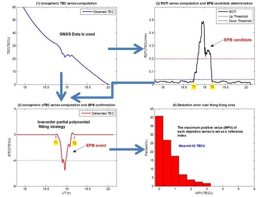
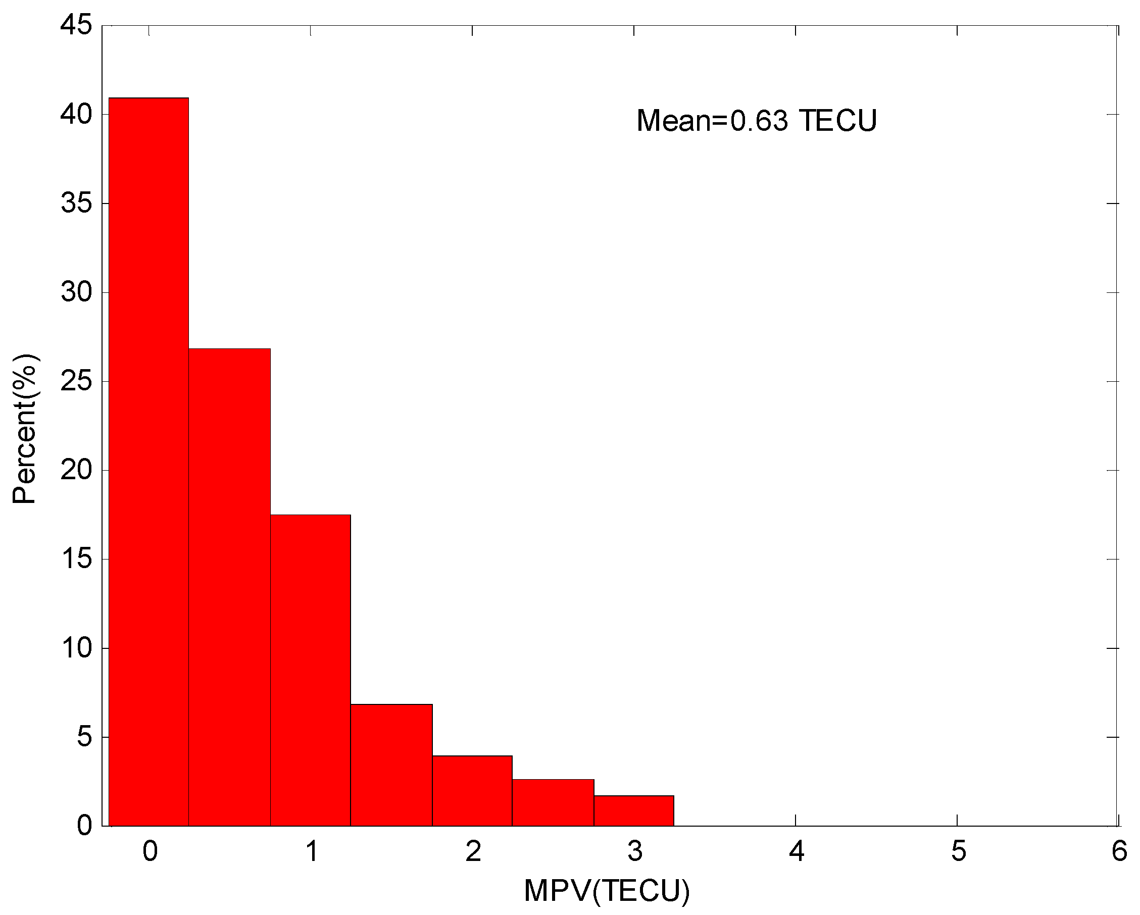
• EPBs generally occur after 20:00 local time and are observed throughout the nighttime and the occurrence during the spring and autumn equinoxes is significantly greater than during the summer and winter solstices, which is also reported in previous studies. In addition, most of the TEC depletion error is smaller than 1.5 TECU and the mean error is 0.63 TECU. These findings suggest that the detection method is feasible and highly accurate.
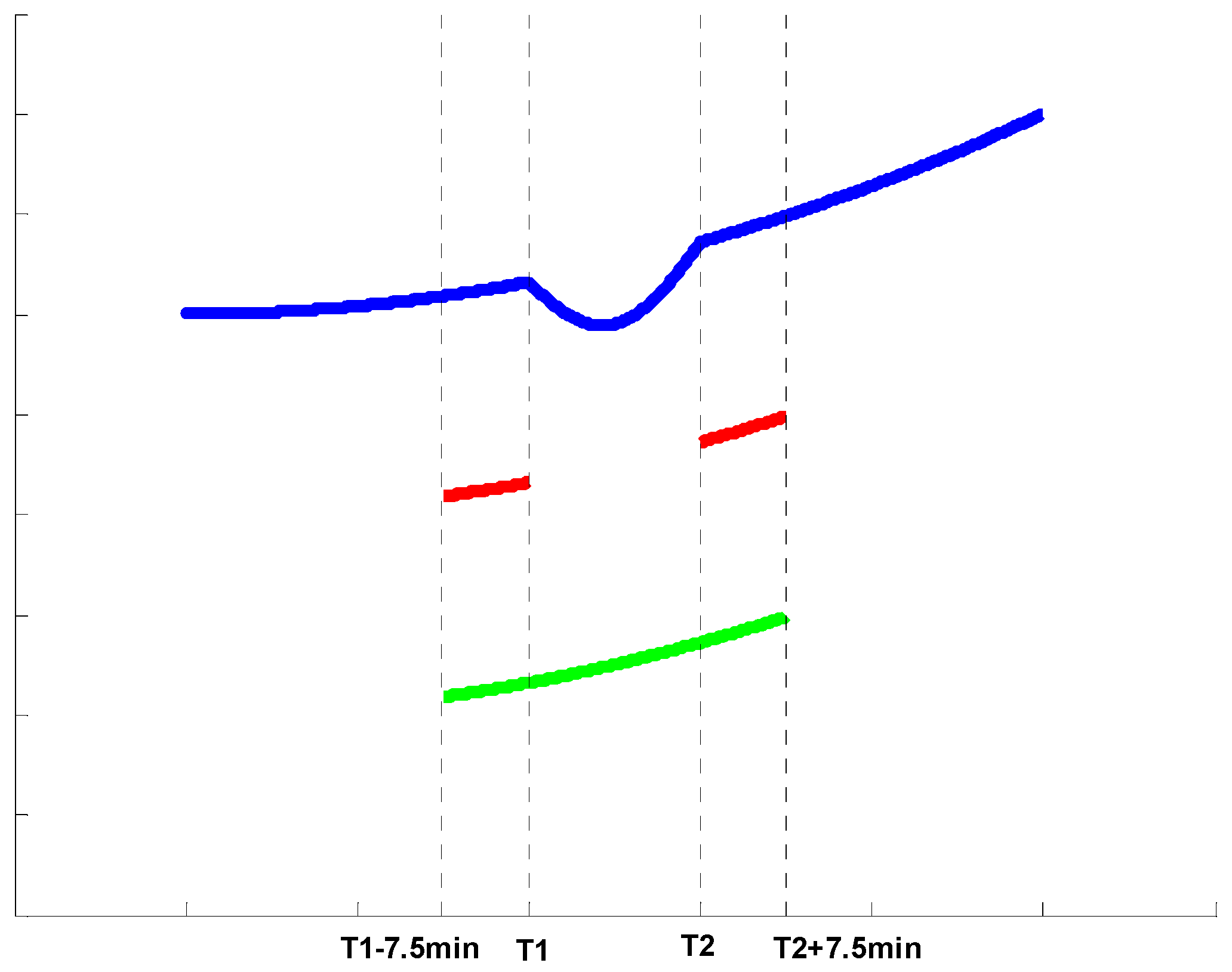
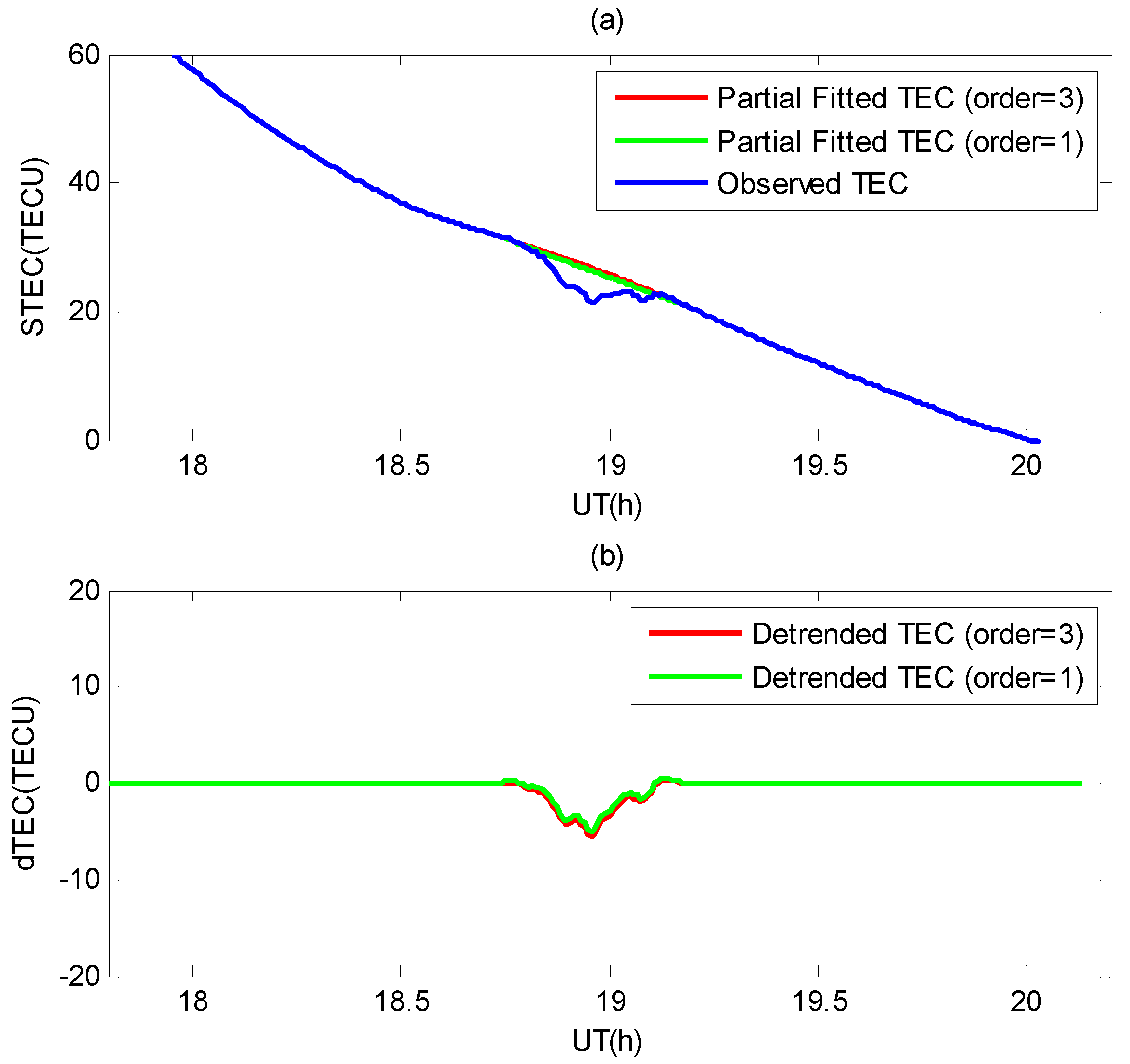
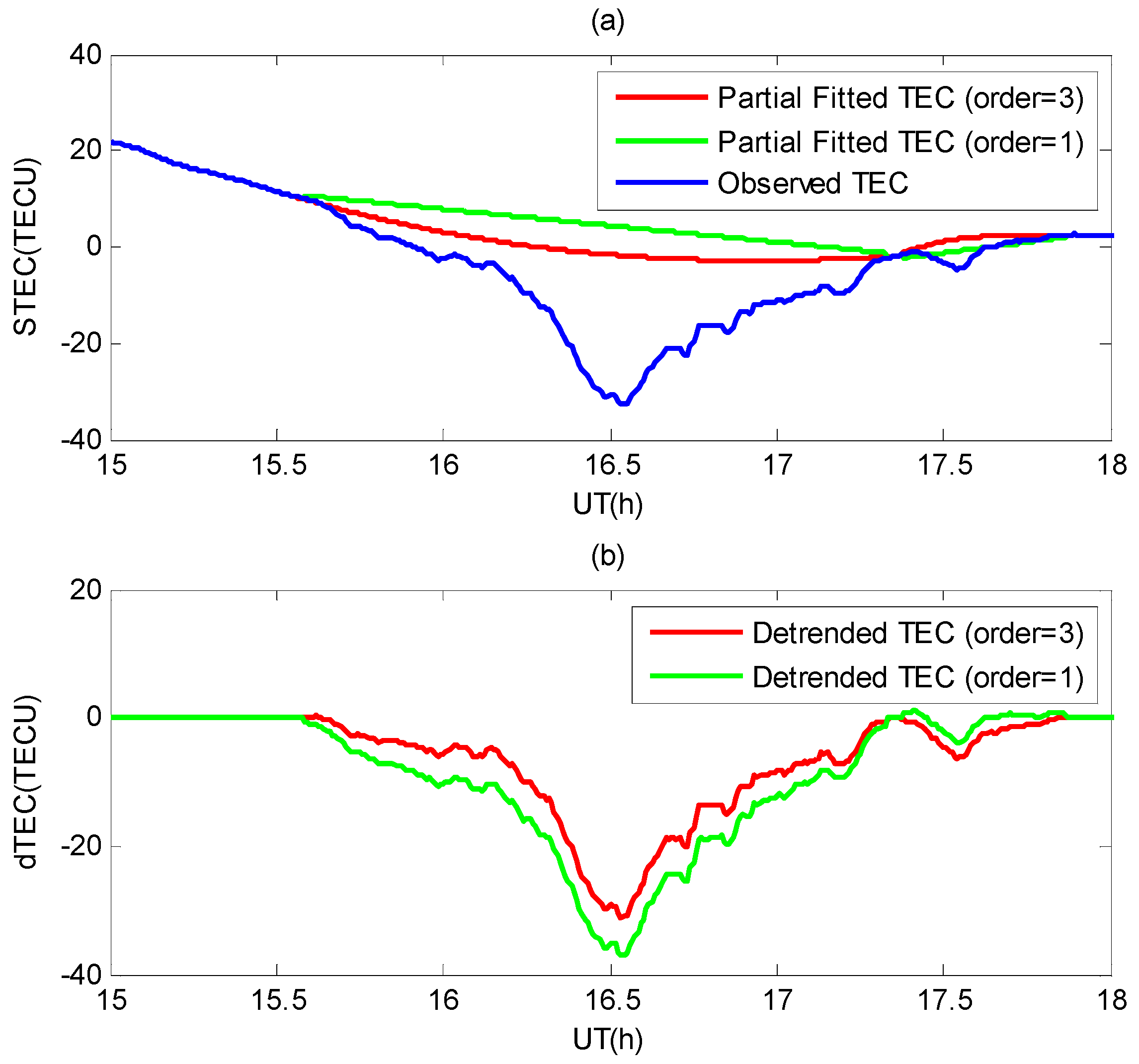
• For short-duration EPB, the fitted TEC series are similar between the third-order polynomial and linear fitting; for long-duration EPB, the fitted TEC series via the third-order polynomial are smoother and more fitting than those via a linear fitting. This suggests that the third-order polynomial fitting is more suitable to fit the background TEC data, and thus adequately extract the TEC depletion by the EPB.

Overall, this method can acquire high-precision EPBs signals which can help to understand the fine characteristics of EPBs and evaluate their effect on GNSS positioning accurately. Here, only the EPBs over the Hong Kong area are tested. In the future, more cases should be investigated to further check this method.

References

1. Sultan, P.J. Linear theory and modeling of the Rayleigh-Taylor instability leading to the occurrence of equatorial spread F. J. Geophys. Res. Space Phys. 1996, 101, 26875–26891. [Google Scholar] [CrossRef]
2. Kelley, M.C. The Earth’s Ionosphere: Plasma Physics and Electrodynamics; Academic Press: Cambridge, MA, USA, 2009. [Google Scholar]
3. Chen, W.; Gao, S.; Hu, C.; Chen, Y.; Ding, X. Effects of ionospheric disturbances on GPS observation in low latitude area. GPS Solut. 2008, 12, 33–41. [Google Scholar] [CrossRef]
4. Huang, C.Y.; Burke, W.J.; Machuzak, J.S.; Gentile, L.C.; Sultan, P.J. DMSP observations of equatorial plasma bubbles in the topside ionosphere near solar maximum. J. Geophys. Res. Space Phys. 2001, 106, 8131–8142. [Google Scholar] [CrossRef]
5. Sobral, J.; Abdu, M.A.; Takahashi, H.; Taylor, M.J.; De Paula, E.R.; Zamlutti, C.J.; De Aquino, M.G.; Borba, G.L. Ionospheric plasma bubble climatology over Brazil based on 22 years (1977–1998) of 630 nm airglow observations. J. Atmos. Sol.-Terr. Phys. 2002, 64, 1517–1524. [Google Scholar] [CrossRef]
6. Abdu, M.A.; Macdougall, J.W.; Batista, I.S.; Sobral, J.H.A.; Jayachandran, P.T. Equatorial evening prereversal electric field enhancement and sporadic E layer disruption: A manifestation of E and F region coupling. J. Geophys. Res. Space Phys. 2003, 108. [Google Scholar] [CrossRef] [Green Version]
7. Burke, W.J. Longitudinal variability of equatorial plasma bubbles observed by DMSP and ROCSAT-1. J. Geophys. Res. 2004, 109, A12301. [Google Scholar] [CrossRef]
8. Kil, H.; Demajistre, R.; Paxton, L.J. F-region plasma distribution seen from TIMED/GUVI and its relation to the equatorial spread F activity. Geophys. Res. Lett. 2004, 31, 179–211. [Google Scholar] [CrossRef]
9. Makela, J.J.; Ledvina, B.M.; Kelley, M.C.; Kintner, P.M. Analysis of the seasonal variations of equatorial plasma bubble occurrence observed from Haleakala, Hawaii. Ann. Geophys. 2004, 22, 3109–3121. [Google Scholar] [CrossRef] [Green Version]
10. Nishioka, M.; Saito, A.; Tsugawa, T. Occurrence characteristics of plasma bubble derived from global ground-based GPS receiver networks. J. Geophys. Res. Space Phys. 2008, 113. [Google Scholar] [CrossRef]
11. Portillo, A.; Herraiz, M.; Radicella, S.M.; Ciraolo, L. Equatorial plasma bubbles studied using African slant total electron content observations. J. Atmos. Sol.-Terr. Phys. 2008, 70, 907–917. [Google Scholar] [CrossRef]
12. Ji, S.; Chen, W.; Wang, Z.; Xu, Y.; Weng, D.; Wan, J.; Fan, Y.; Huang, B.; Fan, S.; Sun, G. A study of occurrence characteristics of plasma bubbles over Hong Kong area. Adv. Space Res. 2013, 52, 1949–1958. [Google Scholar] [CrossRef]
13. Kumar, S.; Chen, W.; Liu, Z.; Ji, S. Effects of solar and geomagnetic activity on the occurrence of equatorial plasma bubbles over Hong Kong. J. Geophys. Res. Space Phys. 2016, 121, 9164–9178. [Google Scholar] [CrossRef]
14. Buhari, S.M.; Abdullah, M.; Yokoyama, T.; Otsuka, Y.; Nishioka, M.; Hasbi, A.M.; Bahari, S.A.; Tsugawa, T. Climatology of successive equatorial plasma bubbles observed by GPS ROTI over Malaysia. J. Geophys. Res. Space Phys. 2017, 122, 2174–2184. [Google Scholar] [CrossRef]
15. Tang, L.; Chen, W.; Louis, O.P.; Chen, M. Study on Seasonal Variations of Plasma Bubble Occurrence over Hong Kong Area Using GNSS Observations. Remote Sens. 2020, 12, 2423. [Google Scholar] [CrossRef]
16. Vargas, F.; Brum, C.; Terra, P.; Gobbi, D. Mean Zonal Drift Velocities of Plasma Bubbles Estimated from Keograms of Nightglow All-Sky Images from the Brazilian Sector. Atmosphere 2020, 11, 69. [Google Scholar] [CrossRef] [Green Version]
17. Magdaleno, S.; Herraiz, M.; Radicella, S.M. Ionospheric Bubble Seeker: A Java Application to Detect and Characterize Ionospheric Plasma Depletion from GPS Data. IEEE Trans. Geosci. Remote Sens. 2012, 50, 1719–1727. [Google Scholar] [CrossRef]
18. Hong Kong Satellite Reference Network. Available online: ftp://ftp.geodetic.gov.hk (accessed on 22 September 2021).
19. Pi, X.; Mannucci, A.J.; Lindqwister, U.J.; Ho, C.M. Monitoring of global ionospheric irregularities using the worldwide GPS network. Geophys. Res. Lett. 1997, 24, 2283–2286. [Google Scholar] [CrossRef]
20. Pi, X.; Iijima, B.A.; Lu, W. Effects of Ionospheric Scintillation on GNSS-Based Positioning. Navig. J. Inst. Navig. 2017, 64, 3–22. [Google Scholar] [CrossRef]
21. Cherniak, I.; Krankowski, A.; Zakharenkova, I. ROTI Maps: A new IGS ionospheric product characterizing the ionospheric irregularities occurrence. GPS Solut. 2018, 22, 69. [Google Scholar] [CrossRef]
22. Sanz, J.; Juan, J.; Hernández-Pajares, M. GNSS Data Processing, Vol. I: Fundamentals and Algorithms; ESTEC TM-23/1; ESA Communications: Noordwijk, The Netherlands, 2013. [Google Scholar]
23. Tang, L.; Li, Z.; Zhou, B. Large-area tsunami signatures in ionosphere observed by GPS TEC after the 2011 Tohoku earthquake. GPS Solut. 2018, 22, 93. [Google Scholar] [CrossRef]
24. Jacobsen, K.S. The impact of different sampling rates and calculation time intervals on ROTI values. J. Space Weather Space Clim. 2014, 4, A33. [Google Scholar] [CrossRef] [Green Version]
Figure 1. Diagram for the partial fitting strategy. The blue line shows the synthesized TEC time series including EPB signals during the period of (T1, T2). The red line shows the data for fitting. The green line shows the fitted TEC time series.
Remotesensing 13 04356 g001
Figure 2. Percent distribution of the rate of TEC variation index (ROTI) calculated for the station HKKT during the year of 2014.
Remotesensing 13 04356 g002
Figure 3. Example of the EPBs detection method in this study using station HKKT and satellite R04 on 28 February 2014. (a) Observed total electron content (TEC, blue line) and partially fitted TEC using third-order polynomial (green line); (b) the rate of TEC variation index (ROTI, black line) and the up threshold (red dot line) and down threshold (blue dot line) for irregularity; (c) detrended TEC (red line). The annotations “T1” and “T2” indicate the initial and end time of EPB.
Remotesensing 13 04356 g003
Figure 4. Temporal distribution of EPBs (top panel) and percent distribution of EPBs occurrence (bottom panel) detected by station HKKT during 2014. “LT” represents local time in Hong Kong.
Remotesensing 13 04356 g004
Figure 5. Percent distribution of the maximum positive value (MPV) by the station HKKT during 2014.
Remotesensing 13 04356 g005
Figure 6. Same example in Figure 3 with first-order and third-order partial polynomial fitting. (a) Observed total electron content (TEC, blue line) and partially fitted TEC using first-order (green line) and third-order polynomial (red line); (b) detrended TEC by subtracting between the observed and partially fitted TEC (green line for first order and red line for third order).
Remotesensing 13 04356 g006
Figure 7. Case of long-duration EPB observed by station HKKT and satellite G09 with first-order and third-order partial polynomial fitting. (a) Observed total electron content (TEC, blue line) and partially fitted TEC using first-order (green line) and third-order polynomial (red line); (b) detrended TEC by subtracting the partially fitted TEC from the observed TEC (green line for first order and red line for third order).
Remotesensing 13 04356 g007
Figure 8. Above two cases with different polynomial orders. The blue line represents the observed TEC, the green and red lines present the partially fitted TEC using third-order and sixth-order polynomial, respectively.
Remotesensing 13 04356 g008