Evaluation of Ionospheric Delay Effects on Multi-GNSS Positioning Performance

Abstract

Ionospheric delay is a significant error source in multi-GNSS positioning. We present different processing strategies to fully exploit the ionospheric delay effects on multi-frequency and multi-GNSS positioning performance, including standard point positioning (SPP) and precise point positioning (PPP) scenarios. Datasets collected from 10 stations over thirty consecutive days provided by multi-GNSS experiment (MGEX) stations were used for single-frequency SPP/PPP and dual-frequency PPP tests with quad-constellation signals. The experimental results show that for single-frequency SPP, the Global Ionosphere Maps (GIMs) correction achieves the best accuracy, and the accuracy of the Neustrelitz TEC model (NTCM) solution is better than that of the broadcast ionospheric model (BIM) in the E and U components. Eliminating ionospheric parameters by observation combination is equivalent to estimating the parameters in PPP. Compared with the single-frequency uncombined (UC) approach, the average convergence time of PPP with the external ionospheric models is reduced. The improvement in BIM-, NTCM- and GIM-constrained quad-constellation L2 single-frequency PPP was 15.2%, 24.8% and 28.6%, respectively. The improvement in convergence time of dual-frequency PPP with ionospheric models was different for different constellations and the GLONASS-only solution showed the least improvement. The improvement in the convergence time of BIM-, NTCM- and GIM-constrained quad-constellation L1/L2 dual-frequency PPP was 5.2%, 6.2% and 8.5%, respectively, compared with the UC solution. The positioning accuracy of PPP is slightly better with the ionosphere constraint and the performance of the GIM-constrained PPP is the best. The combination of multi-GNSS can effectively improve the positioning performance.

1. Introduction

Ionospheric delay effect is one of the main errors in global navigation satellite system (GNSS) positioning, navigation and timing (PNT), and it is normally several or tens of meters although it can exceed 100 m under the severe ionospheric disturbances [1,2]. Nowadays, several ionospheric delay models can be used for real-time or post-processed applications. Among these ionospheric delay models, the Klobuchar model, which is driven by broadcast ephemeris, is widely used by GPS users [3]. The improved Klobuchar model is slightly different and has been specially adapted for Beidou satellites. Similarly, the NeQuick model has also been developed for Galileo users [4]. Additionally, the Neustrelitz TEC Model (NTCM) is a global 2D empirical ionospheric model that can be operated autonomously without external ionospheric measurement [5]. The only driving parameter of the NTCM is the solar radio flux index F10.7. Global Ionosphere Maps (GIMs) are routinely estimated by the International GNSS service (IGS) Analysis Centers (ACs) and have an accuracy of 2–8 TECU (total electron content unit).

With the rapid development of current navigation constellations and construction of more stations, GNSS represents a new era and has wide applications all over the world. In this new multi-frequency and multi-GNSS environment, observations from different signals and constellations are processed together, however, a consideration of the error sources is necessary and mandatory to ensure that the positioning model is consistent. Standard point positioning (SPP) and precise point positioning (PPP) are two types of positioning modes with a stand-alone GNSS receiver that have been used to fulfill different requirements. SPP has been widely used in many fields such as land surveying and vehicle navigation. In the case of the single-frequency SPP approach, the GNSS observations are corrected with existing ionospheric models to ensure a positioning accuracy of meters. The PPP technique has also proved to be an efficient technique due to its high accuracy, global coverage and cost-efficiency. The ionosphere-free (IF) combination is an effective and popular way to eliminate the first order of ionosphere delay in dual-frequency PPP [6]. Another approach is to use the undifferenced and uncombined (UC) observations in dual-frequency PPP processing to extract ionospheric delays and avoid noise amplification [7]. The ionospheric delay is estimated by employing a prior ionosphere model and has the potential to improve positioning performance for wider applications [8,9]. For instance, the experimental tests of [10] showed that the convergence time of dual-frequency PPP was reduced by 30% with the IGS GIM product constraint. Along with dual-frequency PPP, single-frequency PPP has also attracted increasing attention due to its low cast and high accuracy. Similarly, IF combination on a single frequency, known as the Group and Phase Ionospheric Correction (GRAPHIC) can be utilized to eliminate the ionospheric delay in single-frequency PPP [11]. The rank-deficient mathematical problem exists in the GRAPHIC approach, which utilizes the average of the carrier phase and pseudo-range observations. Ionospheric delays can also be estimated simultaneously along with other parameters when proper constraints are given by the ionospheric models. Several studies have been done to improve the convergence time of single-frequency PPP with the GIM [8,12,13]. The quality of ionospheric delay derived from the models will affect the positioning performances. Thus, ionospheric delay is a key issue to resolve in multi-GNSS combined positioning.

In this study, we first present the ionospheric processing strategies for current multi-GNSS single point positioning and summarize the positioning models. Multi-GNSS combined positioning models consist of single-frequency SPP/PPP and dual-frequency PPP. Thereafter, three types of ionospheric correction models, including the broadcast ionospheric model (BIM), NTCM and GIM are introduced for multi-GNSS positioning scenarios. Then, the data and processing strategy is given. A unified time, varying weight, ionospheric scheme for PPP is presented to adapt three ionospheric models. Finally, a comprehensive analysis of the impact of ionospheric delay correction on multi-GNSS performances is performed.

2. Materials and Methods

2.1. Multi-GNSS Positioning Models

The simplest positioning method, SPP is where pseudo-range observations made by a receiver are processed to acquire its position with the orbits of GNSS satellites and their clock offsets, as computed from the broadcast navigation message. Point positioning based on the pseudo-range and phase observations as well as precise orbit and clock products is known as PPP. The quad-constellation GNSS raw pseudo-range and carrier phase observation on the j frequency can be expressed as [14]:

$$p_{r,j}^s={\rho }_r^s+d{t}_r^{}-d{t}^s+T_r^s+I_{r,j}^s+d_{r,j}-d_j^s+{\epsilon }_p$$

(1)

$${\phi }_{r,j}^s={\rho }_r^s+d{t}_r^{}-d{t}^s+T_r^s-I_{r,j}^s+{\lambda }_j{w}_r^s+{\lambda }_j{N}_{r,j}^s+{\lambda }_j(b_{r,j}-b_j^s)+{\epsilon }_{\phi }$$

(2)

where the superscript s denotes a GNSS satellite; the subscript r denotes the receiver; $p_{r,j}^s$ denotes the observed pseudo-range; ${\phi }_{r,j}^s$ is the corresponding carrier phase; ${\rho }_r^s$ denotes the computed geometrical range; $d{t}_r^{}$ is the receiver clock offset; dt^s is the satellite clock offset; $T_r^s$ is the slant tropospheric delay; ${\lambda }_j$ is the wavelength of carrier phase; and $I_{r,j}^s$ is the slant ionospheric delay on jth frequency. It is possible to convert the first order ionospheric delays at different frequencies by $I_{r,j}^s=({\lambda }_j^2/{\lambda }_1^2)I_{r,1}^s$; $d_{r,j}$ and $d_j^s$ are the uncalibrated code delays (UCDs) of the receiver and the satellite on jth frequency; $w_r^s$ is the phase wind-up delay; $N_{r,j}^s$ is the integer ambiguity; $b_{r,j}$ and $b_j^s$ are the uncalibrated phase delays (UPDs) for the receiver and satellites, respectively. ${\epsilon }_p$ and ${\epsilon }_{\phi }$ are the pseudo-range and carrier phase observation noises including multipath, respectively.

For the following statement, we define the notations as:

$$\{\begin{array}{l}{\alpha }_{1,2}^s={(f_1^s)}^2/({(f_1^s)}^2-{(f_2^s)}^2),{\beta }_{1,2}^s=-{(f_2^s)}^2/({(f_1^s)}^2-{(f_2^s)}^2),\\ {\mathrm{DCB}}_{1,2}^s=d_1^s-d_2^s,{\mathrm{DCB}}_{r,1,2}^{}=d_{r,1}^{}-d_{r,2}^{},\\ d_{IF}^s={\alpha }_{1,2}^s\cdot d_1^s+{\beta }_{1,2}^s\cdot d_2^s,d_{r,IF}^{}={\alpha }_{1,2}^s\cdot d_{r,1}^{}+{\beta }_{1,2}^s\cdot d_{r,2}^{},\\ b_{IF}^s={\alpha }_{1,2}^s\cdot {\lambda }_1\cdot b_1^s+{\beta }_{1,2}^s\cdot {\lambda }_2\cdot b_2^s,b_{r,IF}^{}={\alpha }_{1,2}^s\cdot {\lambda }_1\cdot b_{r,1}^{}+{\beta }_{1,2}^s\cdot {\lambda }_2\cdot b_{r,2}^{},\end{array}$$

(3)

where $f_1^s$ and $f_2^s$ are the signal frequency; ${\alpha }_{1,2}^s$ and ${\beta }_{1,2}^s$ are the frequency-dependent factors; ${\mathrm{DCB}}_{1,2}^s$ and ${\mathrm{DCB}}_{r,1,2}^{}$ are the satellite and receiver differential code bias (DCB).

2.1.1. Single-Frequency SPP

It is possible to find a SPP solution based on at least 4 pseudo-range observations and by utilizing dual- or multi-frequency IF combinations, which eliminate the ionospheric delay. For a single-frequency SPP, ionospheric corrections are usually computed by an external model. In general, with m observed satellites and considering the satellite orbits and clocks, satellite timing group delay and atmosphere delays, the single-frequency SPP model can be given for a single epoch as [15]:

$$\left[\begin{array}{c}{p}_{r,1}^{s,1}-{\overline{\rho }}_r^s\\ ⋮\\ p_{r,1}^{s,m}-{\overline{\rho }}_r^s\end{array}\right]=\left[\begin{array}{cc}-{\mathit{u}}_r^s& \mathbf{1}\end{array}\right]\left[\begin{array}{c}\mathit{x}\\ d{\overline{t}}_r^{}\end{array}\right]+\left[{\epsilon }_p^{}\right],{\mathit{Q}}_{\mathit{L}}$$

(4)

$$d{\overline{t}}_r^{}=d{t}_r^{}+d_{r,1}$$

(5)

where ${\overline{\rho }}_r^s$ denotes the geometrical range including the measurement errors; ${\mathit{u}}_r^s$ is the unit vector of the component from the receiver to the satellite; $\mathbf{1}$ is a vector with corresponding rows and one column; x is the vector of the receiver position increments relative to the a priori position; ${\mathit{Q}}_{\mathit{L}}$ denotes the stochastic model of observed minus computed values of observations; The estimable receiver clock $d{\overline{t}}_r^{}$ is a combination of true clock offset plus the receiver hardware delay.

The redundancy of the SPP model is the number of observables minus the number of estimable parameters:$m_s-(3+1)=m_s-4$ (satellites), $m_s$ denotes the number of observables. Hence, the SPP model by least square (LS) is solvable for $m_s\ge 4$.

2.1.2. Single-Frequency PPP

One crucial problem in single-frequency PPP, is that the ionospheric delay cannot be mitigated by the combination of observations on different frequencies. In the GRAPHIC approach, the arithmetic mean of the pseudo-range and carrier phase is considered as the observation where the ionospheric delays are canceled out since the pseudo-range and carrier phase delays have the same values but opposite signs. Thus, the observations with m observed satellites can be expressed as

$$\left[\begin{array}{c}(p_{r,1}^{s,1}+{\lambda }_1{\phi }_{r,1}^{s,1})/2-{\overline{\rho }}_r^s\\ ⋮\\ (p_{r,1}^{s,m}+{\lambda }_1{\phi }_{r,1}^{s,m})/2-{\overline{\rho }}_r^s\end{array}\right]=[\begin{array}{cccc}-{\mathit{u}}_r^s& \mathbf{1}& {\mathit{M}}_{\mathit{W}}& {\mathit{R}}_1\end{array}]\left[\begin{array}{c}\mathit{x}\\ d{\overline{t}}_r^{}\\ Z_w\\ {\overline{N}}_{r,1}^s\end{array}\right]+\left[{\epsilon }_{p,\phi }^{}\right],{\mathit{Q}}_{\mathit{L}}$$

(6)

$$d{\overline{t}}_r^{}=d{t}_r^{}+d_{r,1}/2+{\lambda }_1\cdot b_{r,1}/2$$

(7)

$${\overline{N}}_{r,1}^s=({\lambda }_1(N_{r,1}^s-b_1^s)+d_{IF}^s)/{\lambda }_1/2$$

(8)

where ${\mathit{M}}_{\mathit{W}}$ is the wet mapping function of tropospheric delay; ${\mathit{R}}_1$ denotes the corresponding wavelength of carrier phase to the ambiguity parameters on the first frequency; $Z_w$ is the tropospheric zenith wet delay (ZWD); and ${\overline{N}}_{r,1}^s$ denotes the estimated float ambiguity values on the first frequency.

For the single-frequency UC PPP, the pseudo-range and carrier phase observations with m observed satellites for a single epoch can be written as

$$\left[\begin{array}{c}{p}_{r,1}^{s,1}-{\overline{\rho }}_r^s\\ {\phi }_{r,1}^{s,1}-{\overline{\rho }}_r^s\\ ⋮\\ p_{r,1}^{s,m}-{\overline{\rho }}_r^s\\ {\phi }_{r,1}^{s,m}-{\overline{\rho }}_r^s\end{array}\right]=[\begin{array}{ccccc}-{\mathit{u}}_r^s& \mathbf{1}& {\mathit{M}}_{\mathit{W}}& \mathit{K}& {\mathit{R}}_1\end{array}]\left[\begin{array}{c}\mathit{x}\\ d{\overline{t}}_r^{}\\ Z_w\\ I_{r,1}^s\\ {\overline{N}}_{r,1}^s\end{array}\right]+\left[\begin{array}{c}{\epsilon }_p^{}\\ {\epsilon }_{\phi }^{}\end{array}\right],{\mathit{Q}}_{\mathit{L}}$$

(9)

$$d{\overline{t}}_r^{}=d{t}_r^{}+d_{r,1}$$

(10)

$${\overline{N}}_{r,1}^s=N_{r,1}^s+b_{r,1}-b_1^s-d_{r,1}/{\lambda }_1+d_{IF}^s/{\lambda }_1$$

(11)

where the matrix $\mathit{K}$ denotes the corresponding coefficient of slant ionospheric delay, the element for pseudo-range observation is 1 while the element for carrier phase is −1.

Compared to single-frequency UC PPP, the ionosphere-constrained single-frequency PPP adds virtual ionospheric observations from the external model with their corresponding constraints, which can be expressed as

$$\left[\begin{array}{c}{p}_{r,1}^{s,1}-{\overline{\rho }}_r^s\\ {\phi }_{r,1}^{s,1}-{\overline{\rho }}_r^s\\ ⋮\\ p_{r,1}^{s,m}-{\overline{\rho }}_r^s\\ {\phi }_{r,1}^{s,m}-{\overline{\rho }}_r^s\\ {\tilde{I}}_{r,1}^{s,1}\\ ⋮\\ {\tilde{I}}_{r,1}^{s,m}\end{array}\right]=[\begin{array}{ccccc}-{\mathit{u}}_r^s& \mathbf{1}& {\mathit{M}}_{\mathit{W}}& \mathit{K}& {\mathit{R}}_1\\ \mathit{O}& \mathit{O}& \mathit{O}& \mathit{I}& \mathit{O}\end{array}]\left[\begin{array}{c}\mathit{x}\\ d{\overline{t}}_r^{}\\ Z_w\\ I_{r,1}^s\\ {\overline{N}}_{r,1}^s\end{array}\right]+\left[\begin{array}{c}{\epsilon }_p^{}\\ {\epsilon }_{\phi }^{}\\ {\epsilon }_{ion}^{}\end{array}\right],{\mathit{Q}}_{\mathit{L}},{\mathit{Q}}_{\mathit{I}}$$

(12)

where ${\tilde{I}}_{r,1}^s$ is the virtual ionospheric observation derived from external ionospheric models; $\mathit{O}$ denotes zero matrix; $\mathit{I}$ is the identity matrix; and ${\mathit{Q}}_{\mathit{I}}$ denotes the stochastic model of virtual ionospheric observations.

2.1.3. Dual-Frequency PPP

The IF combination is often utilized for dual-frequency PPP to remove the first order ionospheric delay, which can be expressed as

$$\left[\begin{array}{c}{\alpha }_{1,2}^s\cdot p_{r,1}^{s,1}+{\beta }_{1,2}^s\cdot p_{r,2}^{s,1}-{\overline{\rho }}_r^s\\ {\alpha }_{1,2}^s\cdot {\phi }_{r,1}^{s,1}+{\beta }_{1,2}^s\cdot {\phi }_{r,2}^{s,1}-{\overline{\rho }}_r^s\\ ⋮\\ {\alpha }_{1,2}^s\cdot p_{r,1}^{s,m}+{\beta }_{1,2}^s\cdot p_{r,2}^{s,m}-{\overline{\rho }}_r^s\\ {\alpha }_{1,2}^s\cdot {\phi }_{r,1}^{s,m}+{\beta }_{1,2}^s\cdot {\phi }_{r,2}^{s,m}-{\overline{\rho }}_r^s\end{array}\right]=[\begin{array}{cccc}-{\mathit{u}}_r^s& \mathbf{1}& {\mathit{M}}_{\mathit{W}}& {\mathit{R}}_1\end{array}]\left[\begin{array}{c}\mathit{x}\\ d{\overline{t}}_r^{}\\ Z_w\\ {\overline{N}}_{r,IF}^s\end{array}\right]+\left[\begin{array}{c}{\epsilon }_p^{}\\ {\epsilon }_{\phi }^{}\end{array}\right],{\mathit{Q}}_{\mathit{L}}$$

(13)

$$d{\overline{t}}_r^{}=d{t}_r^{}+d_{r,IF}$$

(14)

$${\overline{N}}_{r,IF}^s=({\alpha }_{1,2}^s\cdot {\lambda }_1\cdot N_{r,1}^s+{\beta }_{1,2}^s\cdot {\lambda }_2\cdot N_{r,2}^s+b_{r,IF}^{}-b_{IF}^s-d_{r,IF}^{}+d_{IF}^s)/{\lambda }_1$$

(15)

where ${\overline{N}}_{r,IF}^s$ denotes the estimated float ambiguity values.

For the dual-frequency UC PPP, the receiver UCD will be absorbed by the receiver clock offset and slant ionospheric delay and the model can be expressed as

$$\left[\begin{array}{c}{p}_{r,1}^{s,1}-{\overline{\rho }}_r^s\\ {\phi }_{r,1}^{s,1}-{\overline{\rho }}_r^s\\ ⋮\\ p_{r,2}^{s,m}-{\overline{\rho }}_r^s\\ {\phi }_{r,2}^{s,m}-{\overline{\rho }}_r^s\end{array}\right]=[\begin{array}{cccccc}-{\mathit{u}}_r^s& \mathbf{1}& {\mathit{M}}_{\mathit{W}}& \mathit{K}& {\mathit{R}}_1& {\mathit{R}}_2\end{array}]\left[\begin{array}{c}\mathit{x}\\ d{\overline{t}}_r^{}\\ Z_w\\ {\overline{I}}_{r,1}^s\\ {\overline{N}}_{r,1}^s\\ {\overline{N}}_{r,2}^s\end{array}\right]+\left[\begin{array}{c}{\epsilon }_p^{}\\ {\epsilon }_{\phi }^{}\end{array}\right],{\mathit{Q}}_{\mathit{L}}$$

(16)

$$\{\begin{array}{l}d{\overline{t}}_r^{}=d{t}_r^{}+d_{r,IF}^{}\\ {\overline{I}}_{r,1}^s={\beta }_{1,2}^s({\mathrm{DCB}}_{1,2}^s-{\mathrm{DCB}}_{r,1,2}^{})\\ {\lambda }_1{\overline{N}}_{r,1}^s={\lambda }_1(N_{r,1}^s+b_{r,1}-b_1^s)+d_{IF}^s-d_{r,IF}^{}+{\beta }_{1,2}^s({\mathrm{DCB}}_{1,2}^s-{\mathrm{DCB}}_{r,1,2}^{})\\ {\lambda }_2{\overline{N}}_{r,2}^s={\lambda }_2(N_{r,2}^s+b_{r,2}-b_2^s)+d_{IF}^s-d_{r,IF}^{}+{(f_1^s/f_2^s)}^2{\beta }_{1,2}^s({\mathrm{DCB}}_{1,2}^s-{\mathrm{DCB}}_{r,1,2}^{})\end{array}$$

(17)

For the ionosphere-constrained dual-frequency PPP, virtual ionospheric observations with their constraints are added and the model can be expressed as

$$\left[\begin{array}{c}{p}_{r,1}^{s,1}-{\overline{\rho }}_r^s\\ {\phi }_{r,1}^{s,1}-{\overline{\rho }}_r^s\\ ⋮\\ p_{r,2}^{s,m}-{\overline{\rho }}_r^s\\ {\phi }_{r,2}^{s,m}-{\overline{\rho }}_r^s\\ {\tilde{I}}_{r,1}^{s,1}\\ ⋮\\ {\tilde{I}}_{r,1}^{s,m}\end{array}\right]=\left[\begin{array}{ccccccc}-{\mathit{u}}_r^s& \mathbf{1}& \mathit{J}& {\mathit{M}}_{\mathit{W}}& \mathit{K}& {\mathit{R}}_1& {\mathit{R}}_2\\ \mathit{O}& \mathit{O}& \mathit{O}& \mathit{O}& \mathit{I}& \mathit{O}& \mathit{O}\end{array}\right]\left[\begin{array}{c}\mathit{x}\\ d{\overline{t}}_r^{}\\ {\mathrm{DCB}}_{r,1,2}^{}\\ Z_w\\ I_{r,1}^s\\ {\overline{N}}_{r,1}^s\\ {\overline{N}}_{r,2}^s\end{array}\right]+\left[\begin{array}{c}{\epsilon }_p^{}\\ {\epsilon }_{\phi }^{}\\ {\epsilon }_{ion}^{}\end{array}\right],{\mathit{Q}}_{\mathit{L}},{\mathit{Q}}_{\mathit{I}}$$

(18)

$$\{\begin{array}{l}{\lambda }_1{\overline{N}}_{r,1}^s={\lambda }_1(N_{r,1}^s+b_{r,1}-b_1^s)+d_{IF}^s-d_{r,IF}^{}\\ {\lambda }_2{\overline{N}}_{r,2}^s={\lambda }_2(N_{r,2}^s+b_{r,2}-b_2^s)+d_{IF}^s-d_{r,IF}^{}\end{array}$$

(19)

In matrix $\mathit{J}$, the element for $p_{r,1}^s-{\overline{\rho }}_r^s$ is set to ${\beta }_{1,2}^s$, and the element for $p_{r,2}^s-{\overline{\rho }}_r^s$ is set to $-{\alpha }_{1,2}^s$, to acquire the corresponding receiver DCB.

2.2. Ionospheric Correction Models

Ionospheric delay models are generally categorized as an empirical model or a mathematical functions model. The former is based on data observed in long-term records and represents the characteristic variation patterns while the latter is fitted by mathematical functions and utilize the actual measured ionospheric delay of a certain area for a period of time.

2.2.1. BIM

The Klobuchar model corrects the ionospheric delay by broadcast ephemeris, which has the advantages of convenient calculation and simple structure [3]. The model considers the periodic and amplitude variations of the ionosphere on a daily scale when setting the parameters, and reflects the characteristic variations of the ionosphere to ensure the reliability of large-scale ionospheric forecasts. The drawbacks of the model are that it is only suitable for the mid-latitude area and it has limited accuracy on the ionospheric delay correction. The input parameters of the Klobuchar model are the eight model coefficients, geodetic latitude and longitude of the GNSS antenna, GPS time, as well as the azimuth and the elevation of the observed satellite.

The improved Klobuchar model is slightly different from the GPS Klobuchar model as it is especially used for Beidou to adapt to the Chinese region. The broadcast parameters of the Beidou Klobuchar are derived based on the monitoring stations in China. The method of Beidou Klobuchar can be found in the Beidou navigation satellite system signal in space interface control document [16].

The NeQuick model is a time dependent ionospheric electron density and three-dimensional model and is applicable for real-time single-frequency correction for the Galileo satellite navigation system. It provides the electron concentration in the ionosphere and total electronic content (TEC) along the ground to satellite ray-path by means of numerical integration [17]. The input parameters of the NeQuick model include the geodetic position of the GNSS antenna, GPS observing time and effective ionospheric level factor AZ determined by three coefficients broadcasted by Galileo ephemeris. The description of the Galileo NeQuick model is available at https://www.gsc-europa.eu/system/files/galileo_documents/Galileo_Ionospheric_Model.pdf.

In the BIM of this study, the GPS and GLONASS satellite ionospheric delay is corrected by the Klobuchar model, the Beidou satellite ionospheric delay is corrected by the improved Klobuchar model, and the NeQuick model is used for Galileo ionospheric delay correction.

2.2.2. NTCM

The NTCM is a user-friendly TEC model that covers all levels and a global scale of solar activity [18]. This empirical approach describes the TEC/ionospheric delay dependencies on the geographic location, local time, and solar irradiance and activity. Considering the irradiation angle of the sun, the TEC variation with the local time is divided into diurnal, semi-diurnal and ter-diurnal harmonic components in the NTCM. The solar activity level is provided by the solar radio flux index F10.7. The 12 model coefficients, together with the covariance matrix in NTCM are fixed and determined by LS adjustment with observation data sets. The standard deviations for the coefficients are utilized to compute 95% confidence intervals. The input parameters of the NTCM are the F10.7 index, day of year, local time in hours, and the geographic and geomagnetic latitude in degrees [5].

2.2.3. GIM

The GIM assumes that the ionosphere is composed of a thin spherical layer at a height of 450 km above the earth’s surface [19]. The GIM provides vertical TEC (VTEC) at certain grid points over the globe. The GIM reconstructed from the predicted and actual measured datasets can be utilized for real-time and post-processed applications, respectively. The vertical electron content at the ionospheric pierce point (IPP) location is generally obtained by interpolation of VTEC values from four neighboring grid points. Hence, space and time interpolations are necessary to obtain the VTEC with high accuracy. The VTEC at an IPP needs to be firstly interpolated between two consecutive maps and then mapped to the slant ionospheric delay. The method for the interpolation and mapping of GIM is explained in detail in [20].

3. Data and Processing Strategy

To evaluate the ionospheric delay effects on multi-GNSS combined positioning performances, datasets from 10 stations of the MGEX network for 1–30 September 2018 (day of year (DOY), from 244 to 273) were selected and utilized for numerical analysis. Figure 1 shows the geographical distribution of the selected MGEX stations. Figure 2 provides the F10.7 values and geomagnetic Kp index for 1–30 September 2018. All of the stations receive quad-system observations from GPS, Beidou, GLONASS and Galileo constellations. The quad-constellation satellite orbits and clock offsets are corrected by the broadcast ephemris provided by MGEX, which is available at ftp://cddis.gsfc.nasa.gov/pub/gps/data/campaign/mgex/daily/rinex3/2018/brdm/, or the precise orbit and clock offset products provided by Deutsches GeoForschungsZentrum (GFZ). The sampling rate of orbit and clock products are 5 min and 30 s, respectively. The detailed data processing strategies for multi-GNSS positioning are shown in Table 1. When integrated multi-GNSS combined positioning is carried out, the additional system time difference is needed for each newly added GNSS system. To maintain the consistency of the pseudo-range and carrier phase observations of the quad constellation, we use b1 to denote observations on the first frequency, b2 to denote observations on the second frequency, and b3 to denote observations on the third frequency. The cut-off angle is set to 7° in this study. The stochastic models of the observations represented by a sinusoidal function and based on the elevation angle of the satellite are utilized to reduce the effect of these elevation angle related errors [21]. The GPS and GLONASS phase observation precision is set to 0.003 m and the GPS code observation precision is set to 0.3 m. To reduce the effect of the inter-frequency bias (IFB) in GLONASS, the GLONASS code observation precision is set to 0.9 m. The Beidou and Galileo code observation precision is set to 0.9 m and 0.4 m, respectively, and the phase observation precision is set to 0.004 m. The LS method is used for SPP data processing and the Kalman filter is utilized in the PPP process of parameter estimation. The tropospheric ZWD is estimated as a random walk process and the receiver clock is estimated as white noise. The time system difference parameters are estimated as constant. The ambiguities are estimated as constant for each epoch.

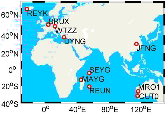
Figure 1. Geographical distribution of the selective MGEX stations.

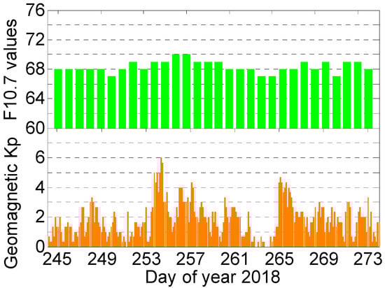
Figure 2. F10.7 values and geomagnetic Kp index on 1–30 September 2018.

Table 1. Data processing strategies for multi-GNSS combined positioning.

Items	Strategies
Data span	1–30 September 2018
Signal Selection	GPS: L1/L2/L5; BDS: B1/B2/B3; GLONASS: G1/G2; Galileo: E1/E5a/E5b
Estimator	SPP: LS PPP: Kalman filter [23]
Observation sampling rate	30 s
Elevation cutoff	7°
Satellite orbit and clock	SPP: broadcast ephemeris provided by MGEX PPP: Fixed by MGEX orbit and clock products
Satellite TGD	Correct using broadcast ephemeris for SPP
Satellite DCB	Correct using MGEX DCB products for PPP
Tropospheric delay	SPP: Modified Hopfield PPP: Modified Hopfield for dry part and estimated for wet part as random-walk process (10−9 m2/s) [24]
Ionospheric delay	Eliminated or estimated as white noise Strategies in Table 2
Relativistic effect	General relativistic models [25]
Sagnac effect	Corrected model [26]
Phase windup effect	Corrected model [27]
Satellite and receiver antenna	Corrected with the values from MGEX and IGS [26]
Tide displacement	Corrected, including solid Earth, pole and ocean tide [26]
Station reference coordinates	IGS SINEX solutions
Station coordinate	Estimated as constants
Receiver clock	Estimated as white noise process (1×105 m2)
Receiver IFB	Estimated as constants or absorbed by receiver clock biases
Phase ambiguities	Estimated as constants for float values

The determination of the weight of virtual ionospheric parameters will affect the ionosphere-constrained PPP performances. In this study, we define the variance of virtual ionospheric parameters as:

$${\sigma }^2=(1+0.2\Delta t)\cdot {\sigma }_{ion}^2\cdot mf{(z)}^2$$

(20)

$$mf(z)={\left[1-{\sin }^{2}z/{(1+H_{ion}/R)}^2\right]}^{-1/2}$$

(21)

where $\Delta t$ denotes the epoch number in the filter processing. ${\sigma }_{ion}^2$ is the mean VTEC spatial variance. H_ion is the height of the ionosphere single layer. R is the average radius of the Earth. Equation (20) indicates that the virtual ionospheric observations are weighed at a relatively larger weight at the beginning, and then the weight gradually decreases to get a better positioning accuracy after convergence [12]. The a priori variance of ionospheric delay is determined by the precision of the ionospheric models. Since the Klobuchar model in BIM can remove the ionospheric delay by more than 50%, the variance for BIM is uniformly set to the square of the corresponding BIM ionospheric correction value [3]. The variance of NTCM is set to 1.22 m² since the model has a root mean square (RMS) deviation of 7.5 TECU [5]. With regard to the GIM, a temporal and spatial correlation function is utilized, which can be expressed as in [22].

$${\sigma }_{ion}^2=\{\begin{array}{l}{\sigma }_{ion,0}^2,t<8ort>20orB>\pi /3\\ {\sigma }_{ion,0}^2+{\sigma }_{ion,1}^2\cos (B)\cos (\frac{t-14}{12}\pi ),other\end{array}$$

(22)

where t is the local time at IPP in hours, B denotes the satellite elevation angle. Since the GIM products have an accuracy of 2–8 TECU, the variance of the zenith ionospheric delay ${\sigma }_{ion,0}^2$ and the zenith ionospheric delay variation ${\sigma }_{ion,1}^2$ are set to 0.09 m² and 0.09 m², respectively.

To obtain the single-frequency SPP solution, three different schemes, ionosphere delay correction with BIM, NTCM and GIM were applied. The rapid GIM products for real-time ionospheric correction were provided by the Center for Orbit Determination in Europe (CODE). For single-frequency PPP, five different schemes including GRAPHIC approach, UC approach, BIM-, NTCM- and GIM-constrained approaches were utilized. For dual-frequency PPP, five schemes including the IF approach, UC approach, BIM-, NTCM- and GIM-constrained approaches, were also applied. The ionosphere processing strategy is summarized in Table 2.

Table 2. Summaries of the ionosphere processing strategy in multi-GNSS positioning.

Constellation	Mode	Schemes	Comment
G, C, R, E	Single-frequency SPP: b1, b2, b3	BIM-corr; NTCM-corr; GIM-corr;	In the BIM, different ionospheric delay models are utilized for their corresponding systems. Klobuchar model (G/R); improved Klobuchar model(C); NeQuick model(E)
G/C
G/R	Single-frequency PPP: b1, b2, b3	GRAPHIC; UC; BIM-cons; NTCM-cons; GIM-cons;
G/E
G/C/R	Dual-frequency PPP: b1-b2;b1-b3	IF; UC; BIM-cons; NTCM-cons; GIM-cons;
G/C/R/E

The abbreviation G, C, R and E represent GPS, Beidou, GLONASS and Galileo, respectively. The abbreviation “corr” and “cons” represent “correction” and “constrained”, respectively.

4. Results and Discussion

4.1. Performance of Single-Frequency SPP

Figure 3 depicts the positioning errors of the CUT0 station on 1 September 2018 for the north (N), east (E) and up (U) component of the b1 and b2 based nine different constellation combinations SPP. It can be seen that the SPP results with b1 and b2 code observations behave similarly. The horizonal error of single-frequency SPP with broadcast ephemeris can reach meter-level, while the vertical error is relatively larger. It is obvious that the accuracy of single-frequency SPP can be improved with multi-GNSS combination. The single-frequency SPP with GIM based ionospheric correction shows the best accuracy, especially in the U direction.

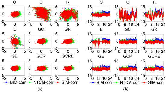
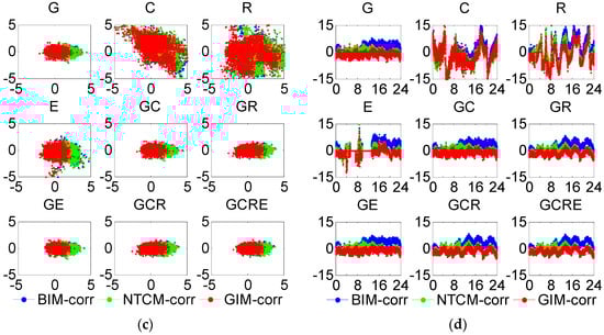
Figure 3. Positioning error scatters of b1 or b2 SPP with different schemes in nine different constellation combinations at station CUT0 (DOY 244/2018, Kp ≈ 0.92) (a) Horizontal error of b1 SPP (b) Vertical error of b1 SPP (c) Horizontal error of b2 SPP (d) Vertical error of b2 SPP. Horizontal error: the horizontal and vertical axes represent the error of the N and E component, respectively (unit: m). Vertical error: the horizontal and vertical axes represent the universal time (unit: hour) and the error of the U component (unit: m), respectively.

The RMS of different single-frequency SPP solutions were calculated, and the mean values of all the tests are summarized in Table 3. As shown in Table 3, the positioning accuracy of multi-GNSS single-frequency SPP with GIM correction performs the best because the GIM is based on the interpolation of the TEC data observed on the selected day and has the highest model accuracy. The solutions from NTCM correction performed better than the BIM correction in the E and U components. Only Beidou, Galileo, GPS/Beidou, and GPS/Galileo b3 SPP solutions were tested, considering that part of the GPS satellites and GLONASS have no triple-frequency signal. For all the single-system single-frequency SPP solutions, Beidou SPP performed the worst, mainly because the satellite orbit and clock offset of the Beidou Geostationary Earth Orbit (GEO) have a relatively lower accuracy. The GPS/Beidou single-frequency SPP achieved slightly better positioning accuracy than the GPS SPP because the Beidou pseudo range observations were assigned less weight than the GPS observations. For the GPS/Galileo b3-based SPP solution, the performance was mainly influenced by the Galileo satellites because few GPS satellites have the b3 signal. For GPS/Beidou/GLONASS/Galileo b1-based SPP, the positioning accuracy was improved by 17.6%, 6.3% and 12.6%, respectively, in the N, E and U components, after the GIM ionospheric correction and compared with the BIM correction. For GPS/Beidou/GLONASS/Galileo b2-based SPP, the positioning accuracy was improved by 28.0%, 12.3% and 31.0%, respectively, in the N, E and U components. For GPS/Galileo b3-based SPP, the positioning accuracy was improved by 30.9%, 21.3% and 16.2%, respectively, in the N, E and U components. For all frequency cases, the multi-GNSS single-frequency SPP performances are improved for more satellites and constellations and the subsequently improved satellite geometry.

Table 3. RMS of single-frequency SPP with BIM, NTCM and GIM based ionospheric correction (unit: m).

Type	Schemes	b1			b2			b3
		N	E	U	N	E	U	N	E	U
G	BIM	2.084	1.680	4.092	2.491	1.806	5.338	-	-	-
G	NTCM	2.152	1.634	3.673	2.634	1.750	4.135	-	-	-
G	GIM	1.704	1.570	3.589	1.768	1.574	3.649	-	-	-
C	BIM	4.455	6.516	8.195	4.685	6.166	8.226	4.096	6.203	7.364
C	NTCM	4.348	6.112	7.621	4.683	5.819	7.423	4.219	5.810	7.055
C	GIM	4.052	6.093	7.717	4.037	4.801	7.475	3.681	5.721	6.990
R	BIM	2.410	2.168	5.422	2.607	2.274	6.382	-	-	-
R	NTCM	2.356	2.061	5.040	2.618	2.156	5.593	-	-	-
R	GIM	2.169	2.022	4.980	2.204	2.080	5.401	-	-	-
E	BIM	3.117	2.802	5.149	3.466	2.935	6.332	3.506	3.033	6.112
E	NTCM	3.190	2.769	4.754	3.804	3.026	5.598	3.767	3.041	5.443
E	GIM	2.773	2.704	4.604	2.936	2.910	5.166	3.025	3.011	2.113
GC	BIM	2.073	1.667	4.077	2.480	1.793	5.324	2.718	3.291	6.770
GC	NTCM	2.141	1.625	3.660	2.624	1.739	4.122	2.823	3.103	5.857
GC	GIM	1.690	1.559	3.578	1.758	1.562	3.636	2.136	2.997	5.413
GR	BIM	1.749	1.396	3.419	2.067	1.495	4.428	-	-	-
GR	NTCM	1.803	1.362	3.108	2.183	1.457	3.498	-	-	-
GR	GIM	1.453	1.312	3.006	1.507	1.318	3.092	-	-	-
GE	BIM	1.697	1.361	3.357	2.052	1.473	4.338	3.081	2.433	5.706
GE	NTCM	1.758	1.326	2.992	2.174	1.429	3.405	2.902	2.187	5.579
GE	GIM	1.368	1.270	2.912	1.433	1.277	2.987	2.129	1.915	4.781
GCR	BIM	1.748	1.394	3.414	2.066	1.493	4.425	-	-	-
GCR	NTCM	1.802	1.361	3.106	2.183	1.455	3.497	-	-	-
GCR	GIM	1.451	1.310	3.005	1.506	1.317	3.091	-	-	-
GCRE	BIM	1.728	1.376	3.381	2.062	1.483	4.429	-	-	-
GCRE	NTCM	1.786	1.344	3.061	2.181	1.445	3.472	-	-	-
GCRE	GIM	1.423	1.290	2.956	1.484	1.301	3.055	-	-	-

“-” means no corresponding combination of results, the same below.

4.2. Performance of Single-Frequency PPP

Table 4 shows the parameter estimation method in single-frequency quad-constellation PPP models, where m, n, p and q denote the satellite number of the GPS, Beidou, GLONASS and Galileo, respectively. The method of eliminating ionospheric parameters is actually equivalent to estimating the parameters [28]. The variance-covariance matrix and the solution vector are identical though they may apply different algorithms [29]. Hence, the GRAPHIC and UC approach are equivalent provided the variance-covariance matrix is transformed according to the law of covariance propagation. The ionosphere-constrained approaches will produce different results for the priori ionospheric information provided by different models.

Table 4. Parameter estimation method in single-frequency quad-constellation PPP schemes.

	GRAPHIC	UC	Ionosphere Constraint
Observed quantity	m+n+p+q	2m+2n+2p+2q	3m+3n+3p+3q
Parameter number	m+n+p+q+8	2m+2n+2p+2q+8	2m+2n+2p+2q+8
Redundancy	−8	−8	m+n+p+q−8
Type of the parameters	Position, receiver clock, ZWD, ambiguity	Position, receiver clock, ZWD, slant ionospheric delay, ambiguity	Position, receiver clock, ZWD, slant ionospheric delay, ambiguity

Figure 4 shows the comparison of b2 single-frequency PPP with different schemes for GPS, GLONASS and GPS/Beidou/GLONASS/Galileo solutions at station MR01 on 2 September 2018. The value errors of respective solutions are shifted by 1 m in order to avoid overlapping. For the single-frequency PPP approach, the positioning filter is considered to have converged when the horizontal components of the error reach 0.3 m and keep within 0.3 m. Because the vertical positioning errors are larger than the horizontal components, the criterion is enlarged to 0.5 m in the vertical direction. The convergence time for N, E and U components are also given and marked in Figure 4. It is obvious that the GRAPHIC and UC approaches have the same convergence time for GPS-only, GLONASS-only and quad-constellation PPP. Besides, the convergence time of ionosphere-constrained PPP solutions is less than the UC solutions at MRO1 for three schemes. The convergence time of the GIM-constrained solutions is the least for its highest model accuracy. The convergence time of quad-constellation single-frequency is reduced for the improvement of spatial geometry with more GNSS satellite compared with the GPS-only solution.

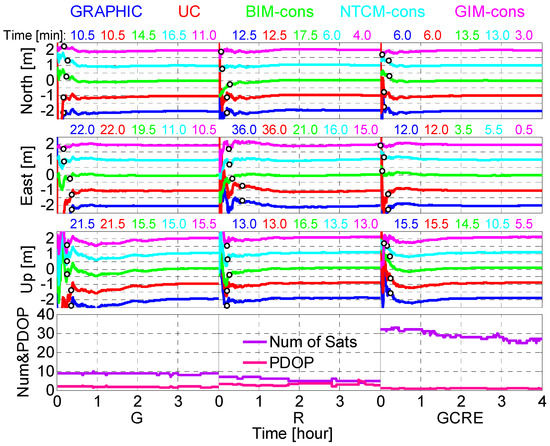
Figure 4. Comparison of positioning error of b2 single-frequency PPP with different schemes for GPS, GLONASS and GPS/Beidou/GLONASS/Galileo solutions at station MRO1 (DOY 245/2018, Kp ≈ 1.17). The corresponding satellite numbers and PDOP values are also shown.

Figure 5 shows the average convergence time of b1, b2 and b3 single-frequency PPP with different schemes on all days over all the test stations. Table 5 summarizes the RMS errors of the single-frequency PPP in multi-constellation combinations, which is calculated from the convergence epoch to the end epoch of a day. The GLONASS-only and Beidou-only solutions clearly perform worse than other solutions, which is caused by the strong correlation between IFBs and slant ionospheric delays in GLONASS and the current distribution and orbit determination accuracy of the Beidou constellation [14]. The results also indicate that the integration of the multi-GNSS can improve the single-frequency PPP performance in terms of convergence time and positioning accuracy. As it is shown in Figure 5 and Table 5, the GRAPHIC and UC approaches have much the same performance for the equivalence of two solutions. By introducing external ionosphere information, the average convergence time of PPP solutions is reduced. For instance, the improvement in convergence time of BIM-, NTCM- and GIM-constrained quad-constellation b2 single-frequency PPP is 15.2%, 24.8% and 28.6%, respectively, compared with the UC solution. The positioning accuracy of the quad-constellation single-frequency PPP can reach 1–3 cm horizontally and 8–9 cm vertically. The improvement in the positioning accuracy of the ionosphere-constrained PPP, for giving higher weighting after convergence, was not significant. The positioning accuracy of the GIM-constrained PPP solutions is the best and NTCM-constrained PPP solutions perform better than the BIM-constrained solutions in the E and U components.

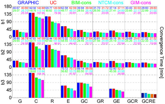
Figure 5. Average convergence time for GPS-only, Beidou-only, GLONASS-only, Galileo-only, GPS/Beidou, GPS/GLONASS, GPS/Galileo, GPS/Beidou/GLONASS and GPS/Beidou/GLONASS/Galileo single-frequency PPP collected at ten stations over thirty days.

Table 5. RMS of single-frequency PPP with IF approach, UC approach, BIM-, NTCM- and GIM-constrained approaches (unit: cm).

Type	Schemes	b1			b2			b3
		N	E	U	N	E	U	N	E	U
G	GRAPHIC	1.664	3.419	9.267	1.818	3.468	6.899	-	-	-
G	UC	1.664	3.419	9.266	1.818	3.468	6.900	-	-	-
G	BIM-cons	1.633	3.990	9.272	1.775	3.924	6.906	-	-	-
G	NTCM-cons	1.667	3.166	9.290	1.826	3.255	6.867	-	-	-
G	GIM-cons	1.642	2.895	9.286	1.824	3.196	6.825	-	-	-
C	GRAPHIC	7.844	10.153	26.782	7.223	9.826	25.374	7.037	9.877	24.515
C	UC	7.859	10.164	26.755	7.217	9.826	25.351	7.040	9.887	24.494
C	BIM-cons	6.318	8.635	25.645	5.672	7.271	24.606	6.540	8.036	23.508
C	NTCM-cons	6.989	8.045	24.288	6.065	6.700	24.302	6.799	7.801	22.575
C	GIM-cons	6.904	7.743	22.011	5.962	6.469	22.314	6.644	7.658	21.717
R	GRAPHIC	4.404	8.003	20.440	4.391	8.582	17.139	-	-	-
R	UC	4.403	8.003	20.503	4.384	8.559	17.142	-	-	-
R	BIM-cons	4.347	8.095	19.267	4.268	8.442	16.998	-	-	-
R	NTCM-cons	4.356	8.090	18.713	4.279	8.449	16.873	-	-	-
R	GIM-cons	4.248	7.941	18.313	3.998	8.373	16.668	-	-	-
E	GRAPHIC	2.717	3.751	7.863	2.486	3.901	8.048	2.939	4.805	8.760
E	UC	2.717	3.753	7.862	2.488	3.901	8.053	2.939	4.805	8.759
E	BIM-cons	2.658	3.777	7.832	2.369	3.932	7.872	2.832	4.592	8.681
E	NTCM-cons	2.758	3.668	7.786	2.530	3.742	7.004	2.917	4.496	8.190
E	GIM-cons	2.521	3.532	7.750	2.315	3.236	6.906	2.666	4.424	7.906
GC	GRAPHIC	1.652	3.387	9.168	1.808	3.430	6.785	3.699	8.942	13.284
GC	UC	1.652	3.387	9.165	1.808	3.429	6.787	3.699	8.941	13.282
GC	BIM-cons	1.628	3.908	9.242	1.746	3.907	6.839	3.304	7.860	12.912
GC	NTCM-cons	1.659	3.162	9.245	1.796	3.166	6.759	3.584	7.430	12.257
GC	GIM-cons	1.632	3.066	9.208	1.793	3.141	6.740	3.106	6.681	12.244
GR	GRAPHIC	1.662	3.418	9.260	1.810	3.461	6.890	-	-	-
GR	UC	1.662	3.417	9.259	1.810	3.461	6.890	-	-	-
GR	BIM-cons	1.618	3.982	9.246	1.765	3.919	6.853	-	-	-
GR	NTCM-cons	1.662	3.159	9.268	1.819	3.172	6.795	-	-	-
GR	GIM-cons	1.631	2.876	9.216	1.821	3.169	6.779	-	-	-
GE	GRAPHIC	1.568	2.905	8.657	1.606	3.123	6.879	2.903	4.489	8.089
GE	UC	1.568	2.905	8.656	1.606	3.122	6.880	2.903	4.489	8.089
GE	BIM-cons	1.542	3.242	8.655	1.568	3.675	6.890	2.806	4.390	8.074
GE	NTCM-cons	1.585	3.007	8.634	1.620	2.899	6.832	2.864	4.164	7.837
GE	GIM-cons	1.543	2.480	8.620	1.618	2.861	6.819	2.829	3.235	7.715
GCR	GRAPHIC	1.651	3.385	9.161	1.711	3.342	6.775	-	-	-
GCR	UC	1.651	3.385	9.159	1.710	3.341	6.777	-	-	-
GCR	BIM-cons	1.550	3.098	9.013	1.664	3.840	6.762	-	-	-
GCR	NTCM-cons	1.591	2.253	8.932	1.734	3.145	6.688	-	-	-
GCR	GIM-cons	1.550	2.047	8.844	1.699	3.129	6.597	-	-	-
GCRE	GRAPHIC	1.557	2.885	8.579	1.599	3.095	6.670	-	-	-
GCRE	UC	1.557	2.885	8.576	1.599	3.094	6.673	-	-	-
GCRE	BIM-cons	1.538	3.035	8.488	1.562	3.507	6.669	-	-	-
GCRE	NTCM-cons	1.578	2.240	8.408	1.610	2.802	6.575	-	-	-
GCRE	GIM-cons	1.541	1.962	8.316	1.599	2.753	6.517	-	-	-

4.3. Performance of Dual-Frequency PPP

Table 6 shows the parameter estimation method in dual-frequency quad-constellation PPP models. The first order of the ionospheric effect has been eliminated in the IF model by the observation combination. However, the combined ambiguities are not integers any more, and the combined observations have higher standard deviations. Similarly, the IF and UC approaches are equivalent as the variance-covariance matrix follows the law of covariance propagation and the ionosphere constrained approaches also leads to different results.

Table 6. Parameter estimation method in dual-frequency quad-constellation PPP schemes.

	IF	UC	Ionosphere Constraint
Observed quantity	2m+2n+2p+2q	4m+4n+4p+4q	5m+5n+5p+5q
Parameter number	m+n+p+q+8	3m+3n+3p+3q+8	3m+3n+3p+3q+12
Redundancy	m+n+p+q−8	m+n+p+q−8	2m+2n+2p+2q−12
Type of the parameters	Position, receiver clock, ZWD, ambiguity	Position, receiver clock, ZWD, slant ionospheric delay, ambiguity	Position, receiver clock, ZWD, DCB, slant ionospheric delay, ambiguity

Figure 6 provides an intuitive comparison of b1/b2 dual-frequency PPP with different schemes for GPS, GLONASS and GPS/Beidou/GLONASS/Galileo solutions at station SEYG on 3 September 2018. The value errors of the respective solutions were shifted by 0.4 m in order to avoid overlapping. The convergence criterion is defined when the component of the error is less than 0.1 m and stays within 0.1 m in the subsequent epochs. During the period 00:00 to 02:00 UTC, approximately 8–10 and 6–8 satellites can be seen at SEYG in each epoch for GPS-only and GLONASS-only PPP and the corresponding variation position dilution of precision (PDOP) is 1.5–2.6 and 1.7–3.0, respectively. The observed satellite number of quad-constellation PPP are between 27 and 32 and the PDOP values are below 1.0 and very stable. It is clear that the IF and UC approaches have almost the same performance at SEYG. The convergence time of ionosphere constraint GPS-only PPP is less than the UC approach thanks to the external ionospheric information at SEYG. The convergence time of ionosphere constrained GLONASS-only PPP is little longer compared with the UC solution, which is mainly caused by the existing IFBs in GLONASS though the pseudo-range observations are assigned a relatively lower weighting. Similarly, the IFBs of GLONASS can also explain why the convergence time of quad-constellation PPP in E and U components is not effectively reduced with the external ionospheric information at SEYG.

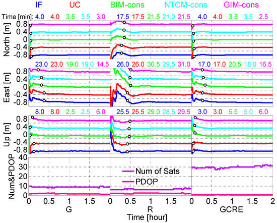
Figure 6. Comparison of positioning error of b1/b2 dual-frequency PPP with different schemes for GPS, GLONASS and GPS/Beidou/GLONASS/Galileo solutions at station SEYG (DOY 246/2018, Kp ≈ 1.92). The corresponding satellite numbers and PDOP values are also shown.

The receiver DCB is estimated as an unknown parameter in the ionosphere-constrained approaches. Figure 7 shows the time series of the estimated GPS, Beidou, GLONASS and Galileo receiver DCB at SEYG. It should be noted that the b1/b3 DCB of GLONASS is not given because the GLONASS has no triple-frequency signal. The multi-GNSS MGEX DCB provided by the Chinese Academy of Sciences (CAS) (available at: ftp://igs.ign.fr/pub/igs/products/mgex/dcb/) is also shown in Figure 7 for reference and comparison, together with the standard deviation (STD) and RMS of corresponding DCB (see top of each panel). It can be seen that the estimated DCB of GIM-constrained approach is much swifter than the other two schemes. Owing to growing weighting for virtual ionospheric observation in the filter process, the existing errors of the ionospheric models have little influence on the positioning accuracy after convergence and are absorbed in the estimable receiver DCB [30]. Hence, as it is shown in Figure 7, this also reflects that the GIM model has the highest accuracy in three models at SEYG.

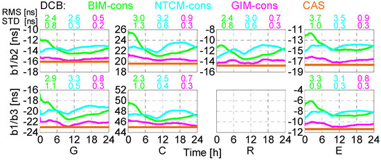
Figure 7. Time series of the estimated receiver DCB at station SEYG (DOY 246/2018).

Figure 8 shows the average convergence time of b1/b2 and b1/b3 dual-frequency PPP with different schemes. Table 7 summarizes the RMS errors of dual-frequency PPP in multi-constellation combinations, the average values of all PPP tests after convergence are calculated. It can be seen that the b1/b2 based PPP performs better than the b1/b3 solutions. The performance of b1/b2 GPS/Beidou and GPS/Galileo PPP differs greatly from the b1/b3 solutions in that only GPS BLOCK-IIF can transmit signals on three frequencies. The positioning accuracy reaches approximately 0.5–2.5 cm in the horizontal and 2–5 cm in the vertical for dual-frequency PPP. Similar to single-frequency PPP, the combination of multi-GNSS speeds up the convergence process and improves the positioning accuracy. For instance, the convergence of quad-constellation b1/b2 GIM-constrained PPP is obviously improved by 40.6% from 13.88 to 8.21 min, compared with the GPS-only solution. The performance of the IF and UC PPP approaches are generally consistent for the equivalence of two models. Introducing different ionospheric models as constraints will reduce the convergence time of PPP schemes in different levels. We can see that the improving average convergence performance for GLONASS-only PPP with ionosphere constraints is the lowest compared with other solutions, where the performances of part stations like the results of Figure 6 may even deteriorate, which is primarily attributed to the existing GLONASS pseudo-range IFBs. The results for dual-frequency ionosphere-constrained GLONASS PPP achieved by [13] is slightly different, which is mainly attributed to different GLONASS code observation precision. In three ionosphere-constrained approaches, the GIM-constrained PPP has the best convergence performance and NTCM-constrained PPP performs better than the BIM-constrained solution. For quad-constellation b1/b2 PPP schemes, the improvement in the convergence time of BIM-, NTCM- and GIM-constrained is 5.2%, 6.2% and 8.5%, respectively, compared with the UC solution. A small but not obvious improvement can be seen in the positioning accuracy with the ionosphere constraint, mainly due to the relatively higher weighting after convergence. The GIM-constrained PPP has the best positioning accuracy in the different schemes.

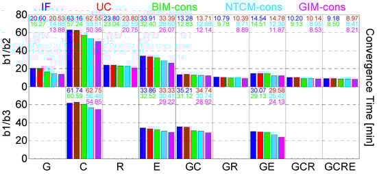
Figure 8. Average convergence time for GPS-only, Beidou-only, GLONASS-only, Galileo-only, GPS/Beidou, GPS/GLONASS, GPS/Galileo, GPS/Beidou/GLONASS and GPS/Beidou/GLONASS/Galileo dual-frequency PPP collected at ten stations over thirty days.

Table 7. RMS of dual-frequency PPP with IF approach, UC approach, and BIM-, NTCM- and GIM-constrained approaches (unit: cm).

Type	Schemes	b1/b2			b1/b3
		N	E	U	N	E	U
G	IF	0.905	1.613	3.147	-	-	-
G	UC	0.907	1.609	3.135	-	-	-
G	BIM-cons	0.878	1.595	3.162	-	-	-
G	NTCM-cons	0.905	1.587	3.159	-	-	-
G	GIM-cons	0.898	1.597	3.148	-	-	-
C	IF	1.435	2.490	5.679	1.560	2.954	5.886
C	UC	1.440	2.526	5.726	1.572	2.956	5.968
C	BIM-cons	1.360	2.374	5.535	1.390	2.464	5.828
C	NTCM-cons	1.387	2.309	5.488	1.398	2.444	5.692
C	GIM-cons	1.377	2.269	5.466	1.340	2.438	5.507
R	IF	0.917	1.873	3.303	-	-	-
R	UC	0.917	1.873	3.302	-	-	-
R	BIM-cons	0.944	1.875	3.472	-	-	-
R	NTCM-cons	0.944	1.889	3.434	-	-	-
R	GIM-cons	0.924	1.878	3.428	-	-	-
E	IF	1.028	1.809	3.566	1.109	2.099	3.364
E	UC	1.025	1.813	3.560	1.080	2.089	3.357
E	BIM-cons	1.040	1.805	3.486	1.066	1.918	3.306
E	NTCM-cons	1.030	1.771	3.404	1.097	1.847	3.318
E	GIM-cons	1.039	1.742	3.111	1.038	1.799	3.308
GC	IF	0.886	1.710	3.066	1.427	2.789	5.405
GC	UC	0.892	1.708	3.056	1.425	2.774	5.393
GC	BIM-cons	0.870	1.581	2.946	1.330	2.367	5.426
GC	NTCM-cons	0.889	1.563	2.957	1.355	2.353	5.238
GC	GIM-cons	0.827	1.529	2.922	1.293	2.307	5.007
GR	IF	0.811	1.525	2.903	-	-	-
GR	UC	0.807	1.523	2.907	-	-	-
GR	BIM-cons	0.790	1.496	2.874	-	-	-
GR	NTCM-cons	0.817	1.487	2.757	-	-	-
GR	GIM-cons	0.771	1.372	2.718	-	-	-
GE	IF	0.871	1.776	3.107	1.053	2.030	3.362
GE	UC	0.864	1.778	3.092	1.054	1.997	3.355
GE	BIM-cons	0.853	1.607	2.920	1.071	1.914	3.445
GE	NTCM-cons	0.854	1.604	2.884	1.077	1.826	3.275
GE	GIM-cons	0.834	1.587	2.868	0.994	1.771	3.247
GCR	IF	0.794	1.513	2.886	-	-	-
GCR	UC	0.787	1.511	2.884	-	-	-
GCR	BIM-cons	0.782	1.428	2.818	-	-	-
GCR	NTCM-cons	0.795	1.408	2.742	-	-	-
GCR	GIM-cons	0.755	1.305	2.701	-	-	-
GCRE	IF	0.777	1.426	2.702	-	-	-
GCRE	UC	0.760	1.393	2.695	-	-	-
GCRE	BIM-cons	0.774	1.345	2.476	-	-	-
GCRE	NTCM-cons	0.778	1.324	2.366	-	-	-
GCRE	GIM-cons	0.676	1.286	2.347	-	-	-

5. Conclusions

To fully evaluate the ionospheric delay effects on multi-GNSS positioning performances, multi-GNSS positioning models for single (b1, b2 and b3) and dual-frequency (b1/b2 and b1/b3) GNSS signals were assessed by different ionosphere processing schemes. The positioning models were extended to SPP or PPP processing with observations from single-, dual-, triple- and quad-constellations. Static datasets collected at ten stations over thirty consecutive days were utilized to evaluate the impact on positioning performance with ionospheric delay models.

Comparative analysis showed that the positioning accuracy of single-frequency SPP with the external ionospheric model correction can obtain meter-level accuracy, and the vertical error is relatively larger than the horizontal components. For single-frequency SPP, the GIM correction solution achieves the best accuracy and the accuracy of SPP with NTCM correction is better than the solution with the BIM correction in the E and U components. The multi-GNSS single-frequency PPP results indicate that the GRAPHIC and UC approaches have the same performance levels. The average convergence time of single-frequency PPP with external ionosphere correction is reduced. Compared with the quad-constellation b2 single-frequency UC approach, the improvement in the convergence time of BIM-, NTCM- and GIM-constrained solutions is 15.2%, 24.8% and 28.6%, respectively. The improvement in positioning accuracy of the ionosphere-constrained PPP is not obvious for the given higher weighting after convergence. The positioning accuracy of the GIM-constrained PPP is the best and NTCM-constrained PPP solutions perform better than the BIM-constrained solutions in the E and U components. For multi-GNSS dual-frequency PPP, the performance of IF and UC solutions are the same. The improvement in convergence time of dual-frequency PPP varies for different constellations. The existing GLONASS pseudo-range IFBs cause the improvement in the GLONASS-only solutions to be the lowest of all schemes. Compared with the quad-constellation b1/b2 UC approach, the improvement in convergence time of the BIM-, NTCM- and GIM-constrained solution is 5.2%, 6.2% and 8.5%, respectively. The positioning accuracy of the GIM-constrained PPP is the best in all positioning schemes. Also, the combination of multi-GNSS can improve the positioning performance for all three positioning schemes.

References

- Jin, S.G.; Jin, R.; Kutoglu, H. Positive and negative ionospheric responses to the March 2015 geomagnetic storm from BDS observations. J. Geod. 2017, 91, 613–626. [Google Scholar] [CrossRef]
- Chen, L.; Yi, W.; Song, W.; Shi, C.; Lou, Y.; Cao, C. Evaluation of three ionospheric delay computation methods for ground-based GNSS receivers. GPS Solut. 2018, 22, 125. [Google Scholar] [CrossRef]
- Klobuchar, J.A. Ionospheric time-delay algorithm for single-frequency GPS users. IEEE Trans. Aerosp. Electron. Syst. 1987, AES-23, 325–331. [Google Scholar] [CrossRef]
- Radicella, S.M. The NeQuick model genesis, uses and evolution. Ann. Geophys. 2009, 52, 417–422. [Google Scholar]
- Jakowski, N.; Hoque, M.M.; Mayer, C. A new global TEC model for estimating transionospheric radio wave propagation errors. J. Geod. 2011, 85, 965–974. [Google Scholar] [CrossRef]
- Odijk, D. Ionosphere-free phase combinations for modernized GPS. J. Surv. Eng. 2003, 129, 165–173. [Google Scholar] [CrossRef]
- Pengfei, C.; Wei, L.; Jinzhong, B.; Hanjiang, W.; Yanhui, C.; Hua, W. Performance of precise point positioning (PPP) based on uncombined dual-frequency GPS observables. Survey Rev. 2011, 43, 343–350. [Google Scholar] [CrossRef]
- Lou, Y.; Zheng, F.; Gu, S.; Wang, C.; Guo, H.; Feng, Y. Multi-GNSS precise point positioning with raw single-frequency and dual-frequency measurement models. GPS Solut. 2016, 20, 849–862. [Google Scholar] [CrossRef]
- Gu, S.; Shi, C.; Lou, Y.; Liu, J. Ionospheric effects in uncalibrated phase delay estimation and ambiguity-fixed PPP based on raw observable model. J. Geod. 2015, 89, 447–457. [Google Scholar] [CrossRef]
- Zhang, H.; Gao, Z.; Ge, M.; Niu, X.; Huang, L.; Tu, R.; Li, X. On the convergence of ionospheric constrained precise point positioning (IC-PPP) based on undifferential uncombined raw GNSS observations. Sensors 2013, 13, 15708–15725. [Google Scholar] [CrossRef]
- Cai, C.; Liu, Z.; Luo, X. Single-frequency ionosphere-free precise point positioning using combined GPS and GLONASS observations. J. Navig. 2013, 66, 417–434. [Google Scholar] [CrossRef]
- Cai, C.; Gong, Y.; Gao, Y.; Kuang, C. An Approach to Speed up Single-Frequency PPP Convergence with Quad-Constellation GNSS and GIM. Sensors 2017, 17, 1302. [Google Scholar] [CrossRef] [PubMed]
- Zhou, F.; Dong, D.; Li, W.; Jiang, X.; Wickert, J.; Schuh, H. GAMP: An open-source software of multi-GNSS precise point positioning using undifferenced and uncombined observations. GPS Solut. 2018, 22, 33. [Google Scholar] [CrossRef]
- Schönemann, E.S.; Becker, M.; Springer, T. A new approach for GNSS analysis in a multi-GNSS and multi-signal environment. J. Geod. Sci. 2011, 1, 204–214. [Google Scholar] [CrossRef]
- Wang, N.; Yuan, Y.; Li, Z.; Huo, X. Improvement of Klobuchar model for GNSS single-frequency ionospheric delay corrections. Adv. Space Res. 2016, 57, 1555–1569. [Google Scholar] [CrossRef]
- CSNO. BeiDou Navigation Satellite System Signal in Space Interface Control Document—Open Service Signal B3I. Version 1.0; China Satellite Navigation Office: Beijing, China, 2018. [Google Scholar]
- Nava, B.; Coisson, P.; Radicella, S.M. A new version of the NeQuick ionosphere electron density model. J. Atmos. Sol. Terrest. Phys. 2008, 70, 1856–1862. [Google Scholar] [CrossRef]
- Hoque, M.M.; Jakowski, N.; Berdermann, J. Ionospheric Correction using NTCM driven by GPS Klobuchar coefficients for GNSS applications. GPS Solut. 2017, 21, 1563–1572. [Google Scholar] [CrossRef]
- Otsuka, Y.; Ogawa, T.; Saito, A.; Tsugawa, T.; Fukao, S.; Miyazaki, S. A new technique for mapping of total electron content using GPS network in Japan. Earth Planets Space 2002, 54, 63–70. [Google Scholar] [CrossRef]
- Schaer, S.; Gartner, W.; Feltens, J. IONEX: The IONosphere Map Exchange Format Version 1. In Proceedings of the IGS AC Workshop, Darmstadt, Germany, 9–11 February 1998. [Google Scholar]
- Witchayangkoon, B. Elements of GPS Precise Point Positioning. Ph.D. Dissertation, Department of Spatial Information Science and Engineering, University of Maine, Orono, ME, USA, 2000. [Google Scholar]
- Gao, Z.; Ge, M.; Shen, W.; Zhang, H.; Niu, X. Ionospheric and receiver DCB-constrained multi-GNSS single-frequency PPP integrated with MEMS inertial measurements. J. Geod. 2017, 91, 1351–1366. [Google Scholar] [CrossRef]
- Kalman, R. A new approach to linear filtering and prediction problems. J. Basic Eng. 1960, 82, 35–45. [Google Scholar] [CrossRef]
- Su, K.; Jin, S. Improvement of Multi-GNSS Precise Point Positioning Performances with Real Meteorological Data. J. Navig. 2018, 71, 1363–1380. [Google Scholar] [CrossRef]
- Kouba, J. A Guide to Using International GNSS Service (IGS) Products; IGS Central Bureau, Jet Propulsion Laboratory: Pasadena, CA, USA, 2009; p. 34. [Google Scholar]
- Gérard, P.; Luzum, B. IERS Conventions; No. IERS-TN-36; Bureau International des Poids et Mesures: Sevres, France, 2010. [Google Scholar]
- Wu, J.T.; Wu, S.C.; Hajj, G.A.; Bertiger, W.I.; Lichten, S.M. Effects of antenna orientation on GPS carrier phase. Astrodynamics 1992, 18, 1647–1660. [Google Scholar]
- Schaffrin, B.; Grafarend, E. Generating classes of equivalent linear models by nuisance parameter. Manuscr. Geod. 1986, 11, 262–271. [Google Scholar]
- Xu, G.; Xu, Y. GPS: Theory, Algorithms and Applications, 3nd ed.; Springer: Berlin, Germany, 2016. [Google Scholar]
- Jin, S.G.; Jin, R.; Li, D. Assessment of BeiDou differential code bias variations from multi-GNSS network observations. Ann. Geophys. 2016, 34, 259–269. [Google Scholar] [CrossRef]
© 2019 by the authors. Licensee MDPI, Basel, Switzerland. This article is an open access article distributed under the terms and conditions of the Creative Commons Attribution (CC BY) license (http://creativecommons.org/licenses/by/4.0/).