Abstract
The wavenumber-frequency spectra of many radar measurements of the sea surface contain a linear feature at frequencies lower than the first order dispersion relationship commonly referred to as the “group line”. Plant and Farquharson, showed numerically that the group line is at least partially caused by wave interference-induced breaking of steep short gravity waves. This paper uses two wave retrieval techniques, proper orthogonal decomposition (POD) and FFT-based dispersion curve filtering, to examine two X-band radar datasets, and compare wave orbital velocity reconstructions to ground truth wave buoy measurements within the field of view of the radar. POD allows group line energy to be retained in the reconstruction, while dispersion curve filtering removes all energy not associated with the first order dispersion relationship. Results show that when group line energy is higher or comparable to dispersion curve energy, the inclusion of this group line energy in phase-resolved orbital velocity reconstructions increases the accuracy of the reconstruction. This increased accuracy is demonstrated by higher correlations between POD reconstructed time series with buoy ground truth measurements than dispersion curve filtered reconstructions. When energy lying on the dispersion relationship is much higher than the group line energy, the FFT and POD reconstruction methods perform comparably.
1. Introduction
In the last several decades, sea clutter has transitioned from a nuisance of operating radar systems in marine environments to a useful tool for quantitative measurements of ocean surface waves. This transition began with the seminal paper by Young et al. in 1985 [1], establishing the Fourier-based dispersion curve filtering method. In the years since this paper was published, techniques derived from Young et al. [1] for calculation of wave statistics have become well established [2,3,4,5]. However, methods and validation for production of phased-resolved wave fields remains an open area of research [6,7,8,9].
Most wavenumber – frequency (k-ω) spectra of radar images of the sea surface exhibit a “group line” feature: a low frequency feature below the first order dispersion relationship that passes through the origin. Numerous explanations exist for the origin of this feature that are wave-related and non-wave related, such as: shadowing, non-linear wave-wave interactions, contamination (e.g., hard targets in the images), turbulence advected by winds, interference-induced wave breaking, and non-linear scattering effects [10,11,12,13,14,15,16]. Recently, in their 2012 study, Plant and Farquharson provide numerical evidence that interference induced wave breaking from the interaction of linear wave fields are a primary source of the group line feature [10]. They demonstrate that the superposition of wind waves and swell can generate steep short gravity waves that break near the local maxima of surface slope, resulting in Doppler measurements of the phase speed of these steep short gravity waves. Such effects as noted by Plant and Farquharson as well as non-linear second order wave-wave interactions may be features that should be accounted for in the generation of instantaneous (phase-resolved) sea surface elevation maps produced by radar [9,13]. However, it is difficult to separate these wave contributions to the group line feature to validate whether they are important to the reconstruction of sea surface elevation maps because other non-wave related effects may also occupy the same frequency-wavenumber space (e.g., shadowing).
In this study, we use a non-Fourier based method, proper orthogonal decomposition (POD), to reconstruct ocean surface orbital velocities from X-band Doppler measurements of the sea surface [17]. This method permits the inclusion of some of the spectral energy in the group line feature in the reconstruction of instantaneous orbital velocities. The inclusion of the group line energy is based on how much it contributes to the overall variance of the measured spatial series [17]. In order to evaluate the importance of group line associated energy to accurate phase-resolved reconstructions of ocean surface wave orbital velocities, the POD results are compared to orbital velocity maps produced using the conventional Fourier-based method (FFT), which filters the k-ω spectra on the linear dispersion relationship for surface gravity waves, and therefore removes all group line features.
We show that inclusion of some portion of the energy in the group line does improve correlation with GPS wave buoy ground truth orbital velocity time series measurements, although this energy does not greatly impact wave statistics (e.g., significant wave height) when computed over approximately 20 min time periods [17]. The results show higher correlation with buoy time series when including group line energy, provided that group line energy is comparable or higher than the energy on the dispersion relationship. These results are demonstrated with experimental data of bimodal seas. The results of this study support the numerical findings of Plant and Farquharson [10] with experimental data, and show that at least a portion of the group line energy is wave field related and contributes to accurate instantaneous phase-resolved sea surface orbital velocities. Presumably by inference, the interference pattern referred to by Plant and Farquharson [10] impacts the wave phasing, and should be included for accurate instantaneous sea surface wave retrievals.
2. Experimental Data
Experimental data for this study was collected during the R/V Melville experiment, which took place from 14 September to 17 September 2013. Details of this experiment are described in Kammerer and Hackett [17]; only relevant details are provided here. The data used in this study was collected using a ship-mounted rotating radar system with a center frequency of 9.41 GHz. It was vertically (VV) polarized, coherent-on-receive [18], and rotated at 24 RPM. Doppler velocity is calculated using the pulse-pair processing method [19]. For noise reduction, the mean of 12 pulse-pairs are taken, generating a Doppler velocity range distribution every 0.86° of rotation (or every 0.006 s). The resulting Doppler velocity distributions are a function of range (r), time (t), and azimuth (φ) (D(r,t,φ)), and cover a range of 960 m at a resolution of 3.75 m with a blanking range of 100 m around the vessel. One “frame” of Doppler data is produced with every full revolution of the radar system.
GPS mini wave buoys developed by the Coastal Observing and Research and Development Center at the Scripps Institution of Oceanography [20] were deployed during the R/V Melville experiment to record ground truth wave data for comparison and validation of radar reconstructions. These buoys were free drifting in and around the area of operation. Only wave buoys in the field of view (FOV) of the radar are used for this study. Figure 1 shows an example of buoy tracks during collection of a radar dataset. The GPS wave buoys have a sample rate of 1 Hz. Prior to time series processing, the buoy data are high pass filtered with a cut off frequency of 0.05 Hz (period of 20 seconds) and de-trended to eliminate non-wave low frequency signals mostly related to the transitioning of GPS satellites. To facilitate comparisons with the radar data, the buoy time series are then low pass filtered and down-sampled to match the temporal resolution of the radar data. Measurement uncertainty and other information about the GPS wave buoys can be found in Drazen [20].
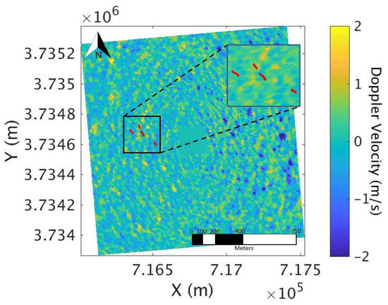
Figure 1.
Tracks from the four GPS wave buoys in the radar field of view during collection of radar dataset 1 are shown in red, overlaid on an example frame of Doppler velocity data. The black box shows a zoom-in of that area.
Two radar datasets from this experiment are used for this study. Datasets were selected based on availability of wave buoys in the field of view of the radar (Table 1) (and for their unique group line features). Dataset 2 was taken approximately 25 min after dataset 1 and during this time winds were decreasing in magnitude (decaying seas). Both datasets were collected under bimodal seas with wind-waves and swell present. Dataset 1 was collected in higher wind speed (15 m/s), and dataset 2 was collected while wind speed was declining (7 m/s). Figure 2 (panels (a) and (b)) shows the k-ω spectrum for each dataset. Dataset 1 has a strong group line feature with a high magnitude of group line energy relative to dispersion curve associated energy, while dataset 2 shows a weaker group line feature relative to dispersion curve associated energy. The primary difference between dataset 1 and 2 is the amount of group line energy relative to dispersion curve associated energy because they were obtained in such close proximity in time to each other. Table 1 shows general environmental statistics for both datasets.

Table 1.
Environmental statistics for both radar datasets used in this study. Shown in the table is the date and time the dataset was collected, as well as the significant wave height (Hs) as measured by the wave buoys, wind speed (Uw) as measured by a shipboard anemometer, root mean squared surface velocity (Vrms) as measured by the wave buoys (averaged over all buoys in the radar FOV), angle between the two wave systems (∆Θ) during dataset collection based on radar derived directional wave spectra, and the number of buoys in the radar FOV.
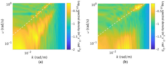
Figure 2.
(a) k-ω Doppler velocity spectrum for dataset 1; (b) k-ω Doppler velocity spectrum for dataset 2. The white dashed line in both panels shows the linear dispersion relationship (adjusted for currents and ship forward speed).
3. Phased Resolved Orbital Velocity Maps
Ocean surface wave orbital velocity maps are produced for all possible frames of radar data using both the POD and dispersion curve filtering methods. The time series of these maps are used to generate time series of orbital velocity by extracting the orbital velocities from each frame at the location where a wave buoy was present. Buoy measured wave orbital velocity time series are compared to orbital velocity time series derived from these radar-based wave orbital velocity maps. Correlation (c) and root mean squared error (Erms) are calculated between the buoy velocity time series and the velocity map derived time series for each method for all available buoys in the FOV of the radar, and these statistics are then averaged across all buoys (see Table 1).
3.1. Pre-Processing
Prior to the POD or FFT wave orbital velocity retrieval methods being performed, pre-processing steps were applied to the radar data. Both datasets were de-trended along range, converted to a Cartesian grid (D(r,t,ϕ) to D(x,y,t)), and georeferenced. Geo-referencing relative to the ship GPS position is performed for each cell of the Cartesian grid so that an accurate cell location of the wave buoys can be identified. Due to sensitivity of the POD method to wave direction [17], the data is rotated such that the dominant wave system is propagating along the direction of the x-axis.
3.2. POD Based Wave Field Extraction
The POD method is applied as described in Kammerer, and Kammerer and Hackett [17,21], which was adapted from Hackett et al. [22]. Only relevant details are repeated here for the reader’s convenience. This method takes one frame of Doppler velocity radar data, D(x,y), and decomposes the signal into a series of orthonormal basis functions (or modes) and spatial coefficients. Mode functions are determined by the best fit to the variance of the data as opposed to being assumed a priori, as in Fourier analysis. As mode number (n) increases, the amount of signal variance accounted for in that mode decreases. The summation of the product of all the mode functions and spatial coefficients results in reconstruction of the original signal.
Because the variance of the Doppler velocity is dominated by the ocean surface wave orbital velocities, a summation of the product of the leading mode functions and spatial coefficients results in a reconstruction of the ocean wave field orbital velocities. This reconstruction method allows energy associated with the group line as well as the dispersion curve to be maintained depending on how much they contribute to the overall variance of the map. POD is performed on frames 16 to N-16, where N is the total number of radar frames in the dataset. This set is selected to maintain the same time series length as the FFT-method, which is described subsequently.
3.3. Conventional FFT Based Wave Field Extraction
The FFT based wave field extraction method is applied as described in Kammerer [21], which was based on the method outlined by Young et al. [1]. After the pre-processing is complete the Doppler radar data is in the form D(x,y,t) with 141 samples in the x and y directions (i.e., a matrix of size 141 × 141 × N). The first 32 frames of radar data are extracted and the x and y dimensions are zero-padded such that the size of D is 256 × 256 × 32. A 3-dimensional FFT is then applied to D. The subsequent Fourier coefficients are then multiplied by a binary dispersion relationship filter (dk(kx,ky,ω)):
where ω is radian frequency, kx is radian wave number in the x-direction, ky is radian wave number in the y-direction, Δω is the radian frequency resolution (0.07 rad/s), W is discrete filter width (W = 1 is used for this study), and σ is the linear deep-water dispersion relationship including current ():
where, is the current, is radian wavenumber, and is gravitational acceleration.
An inverse Fourier transform (IFFT) returns the filtered Fourier coefficients from the spectral domain back to the spatial domain (V(x,y,t)). Only the middle frame of the 3D data stack is extracted and saved as the phase-resolved wave orbital velocity map for the center time of the stack. The 3D stack is then shifted forward by one frame in time for the next set of 32 frames and the process repeats until the last frame in the stack is frame N. The resulting FFT dispersion-filtered time series of phase-resolved wave orbital velocity maps consists of frames 16 to N-16.
4. Time Series Extraction for Buoy Comparisons
For each frame in the time series of wave orbital velocity maps, the spatial coordinates of each buoy in the radar field of view are identified. In order to account for uncertainty in the GPS measurements of the buoy and ship, the velocity of the identified range cell as well as all eight adjacent cells are compared to the buoy wave orbital velocity, and the value closest to the buoy orbital velocity is extracted as the velocity for the radar time series. This process is repeated for each buoy in the field of view of the radar, and for each frame of the radar time series for both the FFT and POD derived ocean surface orbital velocity maps. Figure 1 (Section 2) shows an example of buoy tracks overlaid on one frame of radar data for dataset 1.
Finally, Pearson’s correlation coefficient (c) between each buoy and radar-based time series is computed. Additionally, the root mean squared error (Erms) between the buoy velocity time series, and the POD and FFT reconstructed time series are computed. Both statistics are evaluated for each available wave buoy.
5. Results and Discussion
Figure 3 shows the time series comparisons between the wave buoy, POD, and FFT reconstructions for dataset 1, and Figure 4 shows the time series comparisons for dataset 2. Note, dataset 1 has four buoys in the radar field of view, and dataset 2 has three buoys in the radar FOV (see Table 1, Section 2), with one of the three buoys only being in the field of view for part of the dataset. The number of leading POD modes used for the example reconstructions shown in Figure 3 and Figure 4 was selected to be representative of peak correlation (see Figure 5 and Table 2). Dataset 1 is shown using an n = 32 mode reconstruction and dataset 2 is shown using an n = 6 mode reconstruction. It can be seen in Figure 3 and Figure 4 that the POD reconstructed orbital velocity time series is generally in-phase, and of comparable magnitude to the wave buoy measured velocities for both dataset 1 and 2. The dispersion filtered time series for dataset 1 seems to be of lower magnitude than the wave buoy measured velocities, and out of phase with the buoy measurements at times. However, for dataset 2, the dispersion filtered time series seems to perform in a visually similar way to the POD time series.
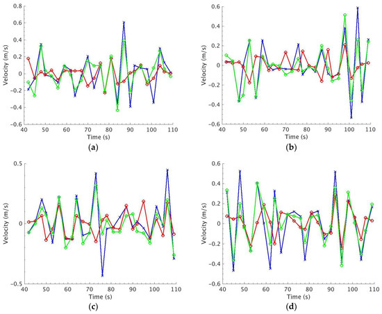
Figure 3.
Time series comparisons between the GPS wave buoys (blue lines), POD reconstructions using the leading 32 modes (n = 32) (green lines), and dispersion filtered reconstructions (red line) for dataset 1. (a) are the time series for wave buoy 279; (b) are the time series for wave buoy 283; (c) are the time series for buoy 286; and (d) are the time series for buoy 289.
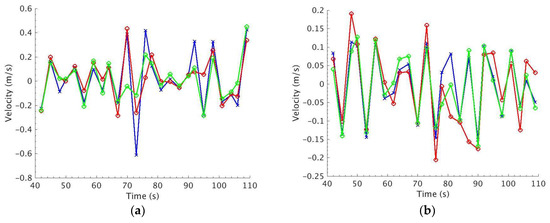

Figure 4.
Time series comparisons between the GPS wave buoys (blue lines), POD reconstructions using the leading 6 modes (n = 6) (green lines), and dispersion filtered reconstructions (red line) for dataset 2. (a) are the time series for wave buoy 279; (b) are the time series for wave buoy 280; and (c) are the time series for buoy 286.
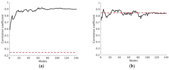
Figure 5.
Average correlation coefficient (c) between POD reconstructed orbital velocity time series and wave buoy orbital velocity time series for each (1 to n) mode reconstruction (black line) and average correlation coefficient between FFT-based dispersion curve orbital velocity time series and wave buoy time series (red dashed line). Correlation coefficients are averaged over all available buoys. (a) shows dataset 1 and (b) shows dataset 2.
Table 2.
Correlation coefficient (c) and Erms for both wave retrieval methods: proper orthogonal decomposition (POD) and dispersion filtering (FFT) for each dataset. For POD, the peak c and minimum Erms are provided with the mode selection (modes 1-n) shown parenthetically.
Figure 5 shows the averaged correlation coefficient between the GPS wave buoy orbital velocity time series and POD reconstructed velocity time series for POD reconstructions using various numbers of modes (1 to n) as well as for the FFT–based reconstructed time series for dataset 1 (a) and dataset 2 (b). Note that correlation coefficients are calculated separately for each available buoy time series and averaged over all buoys. For both dataset 1 and dataset 2, POD reconstructed time series attain above 0.8 correlation coefficient with buoy time series within the leading 10 modes, and peak in correlation at ~0.9. For dataset 1, when the group line energy is stronger relative to dataset 2, POD reconstructions achieve a significantly higher correlation with ground truth wave buoy measurements then the FFT method regardless of the number of modes used in the POD reconstruction. In contrast, for dataset 2, in which dispersion curve energy is higher relative to group line energy, the FFT and POD methods result in similar correlation coefficients regardless of the number of modes used for the POD reconstruction. Furthermore, when spectral energy is limited to primarily dispersion curve associated energy (as in dataset 2), the POD method reaches a correlation “plateau” in fewer modes than when the energy spectra is more complex (i.e., containing group line energy in addition to dispersion curve energy). In summary, POD reconstructed orbital velocity time series correlate highly with buoy-measured wave orbital velocity time series for both datasets, regardless of the group line to dispersion curve energy ratio; when the ratio of group line energy relative to dispersion curve energy is high, the POD method attains significantly higher correlations with buoy measurements than the conventional dispersion curve filtering method. This difference in the correlation coefficients is attributed to the inclusion of group line energy in the POD reconstructions. Nevertheless, the selection of the optimal number of leading modes is non-trivial, but any mode selection achieved higher correlations than dispersion-filtered time series.
The averaged Erms between the reconstructed time series and the ground truth wave buoy time series for both reconstruction methods and datasets is show in Figure 6. Recall, Erms is computed as the root-mean-square of the difference in orbital velocity between the time series. The POD method clearly attains lower Erms than the dispersion curve filtering method for dataset 1 regardless of the number of modes used. In contrast, for dataset 2, Erms is comparable between the methods. The Erms results are consistent with the correlation results shown in Figure 5. When significant group line energy is present, the POD method attains lowers Erms and higher c than the dispersion filtering method (for all mode reconstructions), and when group line energy is low relative to dispersion curve energy, both wave retrieval methods perform comparably. A summary of results for both the correlation and Erms metrics are presented in Table 2.
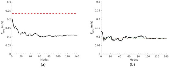
Figure 6.
Averaged root mean squared error (Erms) between POD reconstructed wave orbital velocity time series and ground truth wave buoy measured orbital velocity time series for each (1 to n) mode reconstruction (black line), and between FFT-based dispersion curve filtered time series and wave buoy ground truth (red dashed line) for dataset 1 (a) and dataset 2 (b).
Because the primary difference in the methods is the inclusion of group line energy, and the difference between the datasets is primarily associated with the relative strength of group line energy, we conjecture that the group line energy mostly influences the phasing of the ocean surface wave field and its inclusion in the wave retrieval improves the comparisons with time series buoy data. Figure 7 shows the k-ω Doppler velocity spectrum of the POD reconstructions for datasets 1 and 2 (n = 32 and n = 6 respectively) as well as the k-ω spectra of the dispersion curve filtered reconstructions. The k-ω spectra of the POD reconstructions for both datasets contain energy both associated with the linear dispersion curve and with the group line feature. Note that dataset 1 (a) has high group line energy relative to dataset 2 (b), and the dispersion-filtered reconstructions do not contain any group line energy (c and d). Because the POD reconstructed time series correlate more highly with ground truth buoy time series than the dispersion curve filtered time series for dataset 1 and show smaller Erms, and because the k-ω POD reconstruction spectrum contains significant energy associated with the group line, we surmise that the group line contains energy from the wave field, whose inclusion in wave retrieval contributes to more accurate phase-resolved wave orbital velocity reconstructions.
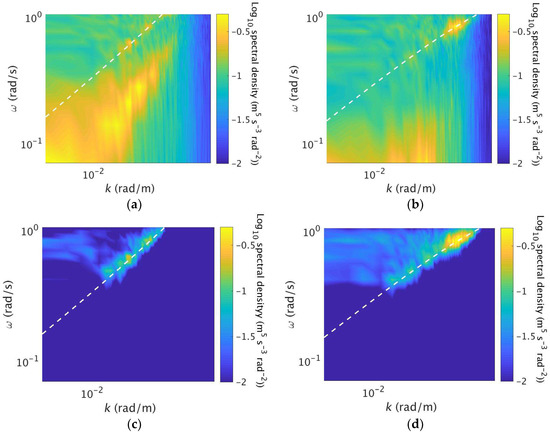
Figure 7.
(a) an example k-ω POD reconstruction spectrum for dataset 1 using 32 modes (n = 32); (b) k-ω POD reconstruction spectrum for dataset 2 using 6 modes (n = 6); (c) k-ω spectrum for the dispersion curve filtered result for dataset 1 and (d) k-ω spectrum for the dispersion curve filtered result for dataset 2. Energy that appears above and to the left of the dispersion curve in (c) and (d) is an artifact of the 3D dispersion cone filtering integrated into 2D for presentation of the figure.
6. Summary and Conclusions
This study has shown that when group line energy is high relative to dispersion curve energy, POD orbital velocity time series attain higher correlation with ground truth wave buoy velocity measurements (and lower Erms) than conventional FFT-based dispersion curve filtering derived wave retrieval. In contrast, when the dispersion curve energy is higher than group line energy, FFT-based dispersion curve filtering attained similar correlation with ground truth measurements than POD; similar Erms is also observed for this dataset. Furthermore, peak correlation between POD-based time series and buoy time series is attained in fewer modes in this case (dataset 2). It is demonstrated that accurate phase-resolved reconstructions of ocean surface wave orbital velocities can be produced from X-band Doppler measurements of the ocean surface using POD and buoy data. More research on automating mode selection is needed in order to use the POD method without optimizing it to buoy data.
The combination of group line energy contained in the POD reconstructed k-ω spectra and the improvement in correlation with ground truth buoy measurements over the conventional dispersion curve filtering method (for dataset 1, with high group line to dispersion curve energy ratio) shows experimental evidence that some portion of the energy associated with the group line feature contains contributions from ocean surface waves. The inclusion of this portion of group line energy increases phase accuracy when the ratio of group line to dispersion curve energy is high. When the ratio of group line energy to dispersion curve energy was lower (dataset 2) performance of the FFT-method to produce phase-resolved maps was more comparable to the POD-based reconstruction method. Thus, the POD method can accurately reconstruct phase-resolved ocean surface velocity maps regardless of the ratio of group line to dispersion curve energy, whereas the conventional FFT-filtering method performs sub-optimally when group line energy is high.
The experimental evidence in this paper supports the numerical results of Plant and Farquharson [10], showing that at least a portion of the group line energy is associated with wave field features, and inclusion of these features contributes to more accurate phase-resolved reconstructions of the ocean surface wave field. The wave field statistics (e.g., those derived from 1D wave spectra) do not appear to be significantly impacted by neglect of the group line energy as shown in Kammerer [21], but the phase-resolved wave field does appear to be impacted as shown in this manuscript. This result implies that the group line mostly influences the phase-resolved wave field, which supports the findings of Plant and Farquharson [10] that attribute the group line feature to wave interference effects that would presumably also affect wave phasing due to the influence of superposition. Further research should examine the significance of the group line energy in phase-resolved wave retrieval for a wider range of conditions.
Author Contributions
Conceptualization, E.E.H.; Methodology, E.E.H. and A.J.K.; Formal Analysis, A.J.K.; Investigation, E.E.H. and A.J.K.; Writing-Original Draft Preparation, A.J.K.; Writing-Review & Editing, E.E.H. and A.J.K.; Supervision, E.E.H.; Project Administration, E.E.H.; Funding Acquisition, E.E.H.
Funding
This research was funded by the Office of Naval Research, grant number [N00014-15-1-2044].
Acknowledgments
The authors would like to thank Joel Johnson and Shanka Wijesundara from The Ohio State University for providing the radar experimental data, and Eric Terrill and Tony DePaulo from the Coastal Observing Research and Development Center at the Scripps Institute of Oceanography for providing the wave data from GPS mini-buoys.
Conflicts of Interest
The authors declare no conflict of interest.
References
- Young, I.R.; Rosenthal, W.; Ziemer, F. A three-dimensional analysis of marine radar images for the determination of ocean wave directionality and surface currents. J. Geophys. Res. Oceans 1985, 90, 1049–1059. [Google Scholar] [CrossRef]
- Nieto Borge, J.C.; Reichert, K.; Dittmer, J. Use of nautical radar as a wave monitoring instrument. Coast. Eng. 1999, 37, 331–342. [Google Scholar] [CrossRef]
- Nieto Borge, J.C.; Rodriguez, G.R.; Hessner, K.; González, P.I. Inversion of marine radar images for surface wave analysis. J. Atmos. Ocean. Technol. 2004, 21, 1291–1300. [Google Scholar] [CrossRef]
- Carrasco, R.; Streßer, M.; Horstmann, J. A simple method for retrieving significant wave height from Dopplerized X-band radar. Ocean. Sci. 2017, 13, 95–103. [Google Scholar] [CrossRef]
- Al-Habashneh, A.; Moloney, C.; Gill, E.W.; Huang, W. An adaptive method of wave spectrum estimation using X-band nautical radar. Remote Sens. 2015, 7, 16537–16554. [Google Scholar] [CrossRef]
- Lyzenga, D. Polar Fourier transform processing of marine radar signals. J. Atmos. Ocean. Technol. 2017, 34, 347–354. [Google Scholar] [CrossRef]
- Lyzenga, D.; Nwogu, O.; Beck, R.; O’Brien, A.; Johnson, J.; de Paolo, A.; Terrill, E. Real-time estimation of ocean wave fields from marine radar data. In Proceedings of the IEEE International Geoscience and Remote Sensing Symposium, Milan, Italy, 31 July 2015; pp. 3622–3625. [Google Scholar]
- Lyzenga, D.; Nwogu, O.; Trizna, D.; Hathaway, K. Ocean wave field measurements using X-band Doppler radars at low grazing angles. In Proceedings of the IEEE International Geoscience and Remote Sensing Symposium, Honolulu, HI, USA, 25–30 July 2010; pp. 4725–4728. [Google Scholar]
- Nwogu, O.; Lyzenga, D. Surface-wavefield estimation from coherent marine radars. IEEE Geosci. Remote Sens. Lett. 2010, 7, 631–635. [Google Scholar] [CrossRef]
- Plant, W.J.; Farquharson, G. Origins of features in wave number-frequency spectra of space-time images of the ocean. J. Geophys. Res. Oceans 2012, 117, C6. [Google Scholar] [CrossRef]
- Dugan, J.P.; Fetzer, G.J.; Bowden, J.; Farruggia, G.J.; Williams, J.Z.; Piotrowski, C.C.; Vierra, K.; Campion, D.; Sitter, D.N. Airborn optical system for remote sensing of ocean waves. J. Atmos. Ocean. Technol. 2001, 18, 1267–1276. [Google Scholar] [CrossRef]
- Dugan, J.P.; Piotrowski, C.C. Surface current measurements using airborne visible image time series. Remote Sens. Environ. 2003, 83, 309–319. [Google Scholar] [CrossRef]
- Dugan, J.P.; Piotrowski, C.C. Measuring currents in a coastal inlet by advection of turbulent eddies in airborn optical imagery. J. Geophys. Res. 2012, 117, 1–15. [Google Scholar] [CrossRef]
- Frasier, S.J.; McIntosh, R.E. Observed wavenumber-frequency properties of microwave backscatter from the ocean surface at near-grazing angles. J. Geophys. Res. 1996, 101, 18391–18407. [Google Scholar] [CrossRef]
- Stevens, C.L.; Poulter, E.M.; Smith, M.J.; McGregor, J.A. Nonlinear features in wave-resolving microwave radar observations of ocean waves. IEEE J. Ocean. Eng. 1999, 24, 470–480. [Google Scholar] [CrossRef]
- Rino, C.L.; Eckert, E.; Siegel, A.; Webster, T.; Ochadlick, A.; Rankin, M.; Davis, J. X-band low-grazing-angle ocean backscatter obtained during LOGAN 1993. IEEE J. Ocean. Eng. 1997, 22, 18–26. [Google Scholar] [CrossRef]
- Kammerer, A.J.; Hackett, E. Use of proper orthogonal decomposition for extraction of ocean surface wave fields from X-band radar measurements of the sea surface. Remote Sens. 2017, 9, 881. [Google Scholar] [CrossRef]
- Smith, G.E.; O’Brien, A.; Pozderac, J.; Baker, C.J.; Johnson, J.T.; Lyzenga, D.R.; Nwogu, O.; Trizna, D.B.; Rudolf, D.; Schueller, G. High power coherent-on-receive radar for marine surveillance. In Proceedings of the 2013 International Conference on Radar, Adelaide, Australia, 16 August 2013; pp. 434–439. [Google Scholar]
- Miller, K.; Rochwarger, M. A covariance approach to spectral moment estimation. IEEE Trans. Inf. Theory. 1972, 18, 588–596. [Google Scholar] [CrossRef]
- Drazen, D.; Merrill, C.; Gregory, S.; Fullerton, A. Interpretation of in-situ ocean environmental measurements. In Proceedings of the 31st Symposium on Naval Hydrodynamics, Monterey, CA, USA, 11–16 September 2016; p. 8. [Google Scholar]
- Kammerer, A.J. The Application of Proper Orthogonal Decomposition to Numerically Modeled and Measured Ocean Surface Wave Fields Remotely Sensed by Radar. Master’s Thesis, Coastal Carolina University, Conway, SC, USA, June 2017. [Google Scholar]
- Hackett, E.E.; Merrill, C.F.; Geiser, J. The application of proper orthogonal decomposition to complex wave fields. In Proceedings of the 30th Symposium on Naval Hydrodynamics, Hobart, Australia, 2–7 November 2014; p. 9. [Google Scholar]


© 2019 by the authors. Licensee MDPI, Basel, Switzerland. This article is an open access article distributed under the terms and conditions of the Creative Commons Attribution (CC BY) license (http://creativecommons.org/licenses/by/4.0/).