Automatic Shadow Detection in Urban Very-High-Resolution Images Using Existing 3D Models for Free Training

Abstract

Up-to-date 3D city models are needed for many applications. Very-high-resolution (VHR) images with rich geometric and spectral information and a high update rate are increasingly applied for the purpose of updating 3D models. Shadow detection is the primary step for image interpretation, as shadow causes radiometric distortions. In addition, shadow itself is valuable geometric information. However, shadows are often complicated and environment-dependent. Supervised learning is considered to perform well in detecting shadows when training samples selected from these images are available. Unfortunately, manual labeling of images is expensive. Existing 3D models have been used to reconstruct shadows to provide free, computer-generated training samples, i.e., samples free from intensive manual labeling. However, accurate shadow reconstruction for large 3D models consisting of millions of triangles is either difficult or time-consuming. In addition, due to inaccuracy and incompleteness of the model, and different acquisition time between 3D models and images, mislabeling refers to training samples that are shadows but labeled as non-shadows and vice versa. We propose a ray-tracing approach with an effective KD tree construction to feasibly reconstruct accurate shadows for a large 3D model. An adaptive erosion approach is first provided to remove mislabeling effects near shadow boundaries. Next, a comparative study considering four classification methods, quadratic discriminant analysis (QDA) fusion, support vector machine (SVM), K nearest neighbors (KNN) and Random forest (RF), is performed to select the best classification method with respect to capturing the complicated properties of shadows and robustness to mislabeling. The experiments are performed on Dutch Amersfoort data with around 20% mislabels and the Toronto benchmark by simulating mislabels from inverting shadows to non-shadows. RF is tested to give robust and best results with 95.38% overall accuracy (OA) and a value of 0.9 for kappa coefficient (KC) for Amersfoort and around 96% OA and 0.92 KC for Toronto benchmarks when no more than 50% of shadows are inverted. QDA fusion and KNN are tested to be robust to mislabels but their capability to capture complicated properties of shadows is worse than RF. SVM is tested to have a good capability to separate shadow and non-shadows but is largely affected by mislabeled samples. It is shown that RF with free-training samples from existing 3D models is an automatic, effective, and robust approach for shadow detection from VHR images.

1. Introduction

1.1. Motivation

Automatic 3D city model reconstruction has been intensively investigated in recent decades. A detailed review can be found in [1]. Airborne LiDAR point clouds are widely used for obtaining geometric information, especially for buildings, while very-high-resolution (VHR) images and topographic maps help to segment the scene to give texture or semantics to the city model [2]. Point clouds can be created from image matching [3,4], but images should have good radiometric quality and large image overlap to result in accurate and reliable information for urban modeling. LiDAR point clouds are often available for urban areas; however, they are quite expensive, so the updating rate is low, especially at state or national level. For example, the national point clouds in the Netherlands, Actueel Hoogtebestand Nederland (AHN), have an update rate of 5–10 years. This updating rate does not meet the requirements of many applications. For example, in the context of disaster management, up-to-date and accurate 3D models are of utmost importance [5]. To keep 3D models up to date, VHR aerial images are the first choice for two reasons: first, VHR aerial images are often updated annually. Second, their high spatial resolution, even to the centimeter, provides rich and valuable geometric and color information. Instead of reconstructing 3D models from scratch, VHR images can be used to detect changes in 3D models by considering that urban areas are not expected to change a lot in a year. To detect changes using images, shadows should be considered and detected both from a geometric and a color perspective. Shadow is actually one kind of geometric information which has been used for detecting buildings from VHR images in [6]. Furthermore, shadows reconstructed from existing 3D models differing from shadows detected from newly acquired images could indicate changes. In this context, both miss- or over-detection of shadows immediately results in miss- or over-detection of changes. On the other hand, radiometric distortions in shadows produce serious false alarms when detecting changes from colors. Shadows are either used for reducing false alarms from change detection or compensating to reveal real colors for change detection. Therefore, our study concentrates on detecting shadows from VHR images in urban areas.

1.2. Related Work

Existing literature presents three main categories of shadow detection [7,8]: property-based, supervised learning-based and model-based. Property-based methods do not need any prior knowledge and are often combined with automatic thresholding. They focus on exploring spectral properties to identify shadows. Shadow properties have been studied intensively [7,9,10] and are summarized into four properties:

• Shadows have low radiance due to obstruction of direct sunlight.
• Radiance received from shadow areas decreases from short (blue-violet) to long (red) wavelength due to scattering effects.
• In urban canyons, reflection effects of surroundings cannot be ignored in the shadow area.
• Radiance received from shadow areas is material-dependent.

The first two properties explain why property-based methods work reasonably well in many studies. According to property 1, shadows tend to have low RGB or intensity values. Referring to property 2, in RGB images, shadows should have higher blue than their counterpart in the sun, while non-shadows receive direct light with more red and green radiation. Tsai (2006) [9] discusses the ratio of hue over intensity to combine these two properties to enlarge the difference between shadow and non-shadow. With high hue (more blue) and low intensity values, shadows are expected to have much higher ratio values than non-shadows. The $HSI$ color space is tested with best performance in Tsai’s work and the ratio is defined as $\frac{H+1}{I+1}$, where H and I present hue and intensity value in HSI color space. Finally, a thresholding method [11] was used to separate shadows from non-shadows. Based on this finding, a new ratio is designed [10] to stretch the gap between shadow and black objects. However, the other two properties which affect the efficiency of the first two properties are not considered. According to property 3, if the material of a surrounding object is highly reflective, shadows may receive high reflection which can be confused with dark objects. Referring to property 4, the red value of reddish objects under shadow is largely reduced, but they may have very different hue values depending on the red value or blue value is a little higher. If red is a bit higher than blue, the hue is much smaller than the opposite situation. Due to the high sensitivity of hue, the effectiveness of property 2 is adversely affected.

Supervised learning is expected to have better performance in shadow detection in images by learning the characteristics of shadows in complex scenes. Much research has applied supervised learning on airborne VHR images and natural images in computer vision. The shadows in these images share the same characteristics of all four properties described. A support vector machine (SVM) with a polynomial kernel of degree 3 performs well for natural RGB images [12]. Apart from RGB features, the texture features from texton histograms are used with SVM for classifying natural images [13]. In VHR images, Lorenzi et al. [8] extract texture features from a wavelet transform for SVM to detect shadow. As textures in shadows are not very informative, RGB features are more often used for shadow detection. However, supervised approaches require lots of manual work to generate good training examples with large varieties. In [14], shadow detection is performed using a limited amount of training samples. Two Gaussian mixture models (GMM) were built for shadow and non-shadow regions respectively from strokes drawn manually. Mean-shift clustering was applied to segment the whole image. Finally, the clusters are classified based on which GMM they are similar to. The goal of clustering is to remove small dissimilarities from pixels in order to limit the training samples to describe these small details. However, the result is strongly dependent on cluster and GMM parameters. It is hardly suitable for different environments. An advanced closed-form solution is provided in [15] to reduce the large amount of user input to identify shadows from regular images by image matting. The idea is to use a local smoothness constraint to propagate the characteristics of shadows (foreground) and non-shadow (background) from user inputs to other unknown regions. This approach works well for different environments with limited manual samples, but manual work and variation in user input are still required. As shadows are strongly dependent on the environment, training samples extracted from one image may have a very bad generalization capability compared to images from different areas or different time. This implies a large amount of work to select training samples for the images from which we want to detect shadows.

Model-based methods use an existing 3D model or DSM to reconstruct shadows with camera parameters and sun position by ray tracing [16] or z-buffers [17]. The z-buffer approach uses two depth maps to determine whether a pixel in the DSM can be seen by the sun and by the camera, respectively. However, this approach has problems related to how to map the pixel from one depth map to another. Ray tracing can produce very accurate results for 3D models, either in vector or voxel presentation. However, ray tracing is time-consuming. It is mandatory to create a data structure for 3D models to apply ray tracing to a large 3D model, but this topic is rarely discussed in remote-sensing research. Furthermore, a 3D model is often not very accurate and misalignment occurs between 3D data and image as they are obtained from different resources and geo-referenced independently. Mismatches often appear near the boundary of reconstructed images. In [16], the interior of large shadows or non-shadows in the reconstructed images is automatically selected as free-training examples by an erosion morphological filter. A SVM classifier is then applied to improve shadow detection. Wang et al. [18] adopted image matting [15] using skeletons of (non-)shadow regions as input to detect shadows from mislabels caused by moving cars, trees, and water. The paper does not assess the number of mislabels and robustness of the methods to mislabeling. More importantly, these two papers did not consider that models and images are often taken at different times. With more than one year difference, the changed buildings and trees provide many mislabeling samples, which is mandatory to consider.

1.3. Contribution of Our Study

In urban VHR images, the effects of shadow properties 3 and 4 described above are not trivial. As shown in Figure 1a,b, many dark roofs have RGB values similar to those from facades and roads under shadow. With the colors displayed in Figure 1c, this effect is more obvious. Many pixels in reddish objects show similar intensities with even higher value in red than the dark objects in the sunlight. A property-based approach that only considers property 1 and 2 cannot capture these complicated shadow properties, but supervised learning approaches which are data driven are expected to find reasonably good boundaries to separate different classes. However, the generalization ability of applying the classifier trained in one place to classify shadows in another place is affected by illumination conditions, environment, and object material. Therefore, training samples should be selected from each image, which is labor intensive. Model-based methods can provide free, large, and various training samples from the image which needs to be classified. However, the training samples indicated from the reconstructed shadow images are not all labeled correctly. If the samples are used for training classifiers, the effect of these mislabeled training samples is called mislabeling.

The contributions of our paper are as follows:

• We provide a fully automatic, effective, and robust approach of shadow detection in VHR images using existing 3D city models for shadow reconstruction to provide free-training samples. The reconstructed shadow image is used label VHR images for providing free training, meaning that training samples are generated by a computer and free from manual labor.
• We conduct a comparative study on how machine learning methods are affected by mislabeling effects introduced by free-training samples and their ability to detect complicated shadows.

The remainder of the paper is organized as follows: Section 2 describes study area and data preparation. Section 3 discusses the change detection workflow and explains four comparative methods. Section 4 analyzes and discusses the performed experiments. The last section concludes the paper.

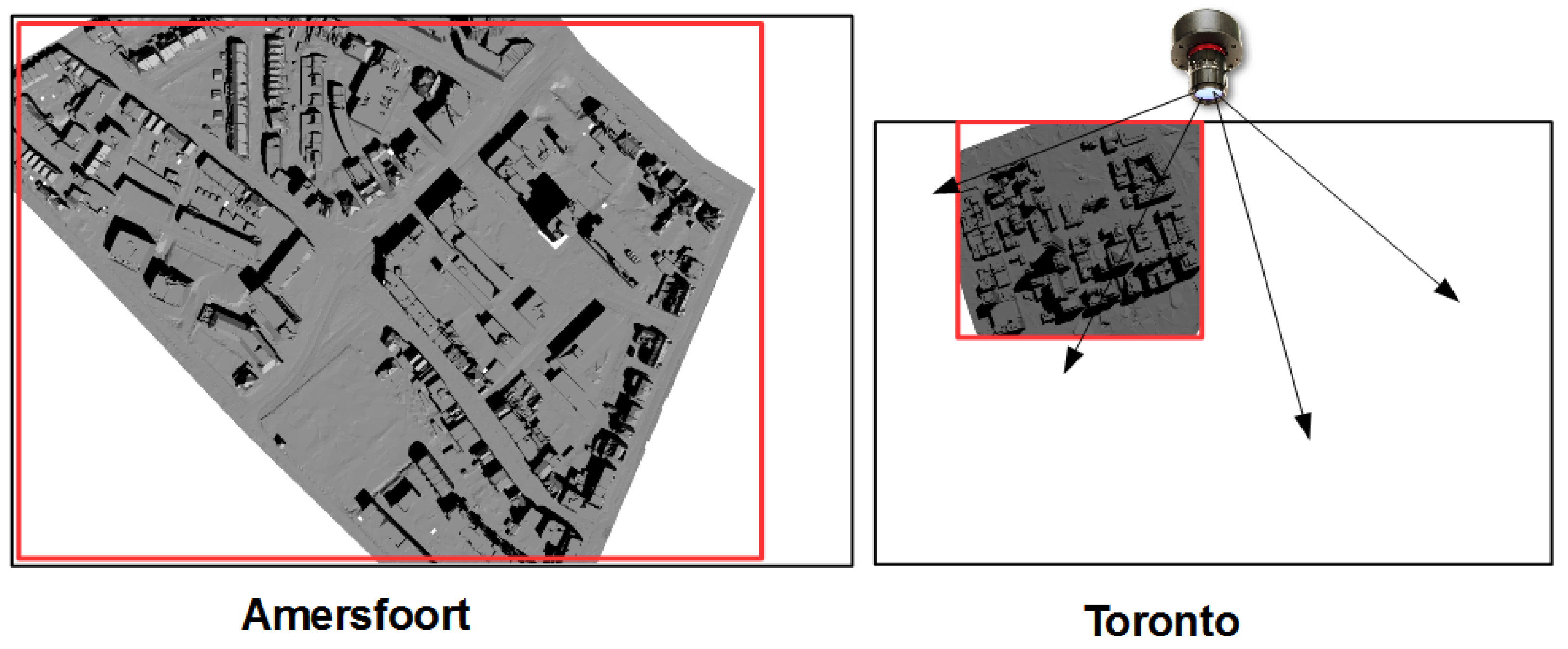
2. Study Area and Data Preparation

The study areas are in Amersfoort, the Netherlands and Toronto, Canada. The Toronto dataset is from an ISPRS benchmark test. The data required for the two study areas are the same: an existing 3D city model and a VHR image.

2.1. 3D model Generation

A 3D triangular model of Amersfoort is created automatically by combining a topographic map and LiDAR point clouds acquired around the same time using software provided by the University of Twente [19]. Four object classes are aggregated from classes defined in BGT, the Dutch large-scale topographic maps and included in the 3D model [19]: water, road, terrain and building. These objects together form a seamless terrain which is important for reconstructing shadows on the ground. The models are triangulated based on simplification rules specific for different classes. For example, roads are regarded as planes and can be constructed by triangulating the polygonal vertices from the map with heights determined by a local plane fitting all LiDAR points inside the polygon. Building polygons from the map are used for a constraint triangulation for buildings, and their roofs are simplified from a triangulated mesh by considering the planarity of adjacent triangles. Details can be found in [19] and the 3D model is displayed in the left image of Figure 2a. The 3D model of Toronto is created by extruding reference 3D roof planes. The reference roofs are manually created for evaluating 3D building extraction algorithms. In this paper, they are regarded as an existing resource for constructing a 3D city model. Ground points are first segmented from LiDAR point clouds using a progressive morphological filter [20]. As no topographic map is available for simplifying ground triangles, a voxel-grid filter which replaces points in a voxel with the voxel centroid is used to simplify ground points for triangulation. The 3D buildings are obtained by extruding roof planes to the ground using FME software [21], Safe Software Inc. As shown in the right image of Figure 2a, this 3D city model has only two classes: terrain and building. There are several reasons for not considering trees in two models: (1) trees are difficult to accurately model from airborne LiDAR. Tree points are often sparse, and many points penetrate into leaves and even reach to trunks and ground. (2) if the image has an acquisition time different from LiDAR, the status of trees is different. The numbers of triangles in the models of Amersfoort and Toronto are 429,904 and 30,770, respectively. The areas covered by each model are around 0.2 km${}^2$. As the automatically generated buildings in Amersfoort are not represented by optimal triangles such as those manually created for Toronto; the Amersfoort model has more triangles than the Toronto model.

2.2. VHR Image Description

The VHR aerial images from Amersfoort and Toronto are taken by a Microsoft Vexcel UltraCam-Xp with $3.5$ cm spatial resolution and an UltraCam-D camera with 15 cm spatial resolution, respectively. The data channels of Amersfoort and Toronto are RGB. The image size per frame is 11,310*17,310 and 7500*11,500 for Amersfoort and Toronto, respectively. On all the images, a bundle adjustment is performed by ground control points to provide a file with camera parameters. The back-projection error of using these parameters is less than 1 pixel. The 3D model for Amersfoort is created from LiDAR data and maps acquired in 2008, while the images were acquired in April 2010. There were many building constructions during these two years. No explicit acquisition time of the images from Toronto is known. However, by visually checking, very limited changes of buildings are found between model and images. The trees are thin and sparse and with the accurate reference roofs, the reconstructed shadows match the shadows in the image very well. The VHR images corresponding to the 3D models are shown in red polygons of Figure 2b.

The two datasets are chosen for two reasons. (1) The shadows properties in both areas are complicated. In Amersfoort, the reflectance of shadows casted on many reddish roads are material-dependent as shown in Figure 1. Apart from material problems, the Toronto area has many high-rise buildings. Shadows receive light reflected from glass walls in the buildings, resulting in shadows with a high reflectance. This requires a method that is capable of robustly capturing these complicated properties to best separate shadows and non-shadows in different environments. (2) In Amersfoort, due to time differences and because tree models are not incorporate, many mislabeled samples are included. The Toronto model matches the image very well, so the training samples are in general correctly labeled. The comparison of shadow detection on these two datasets can evaluate the robustness of methods on mislabeling effects.

3. Shadow Detection

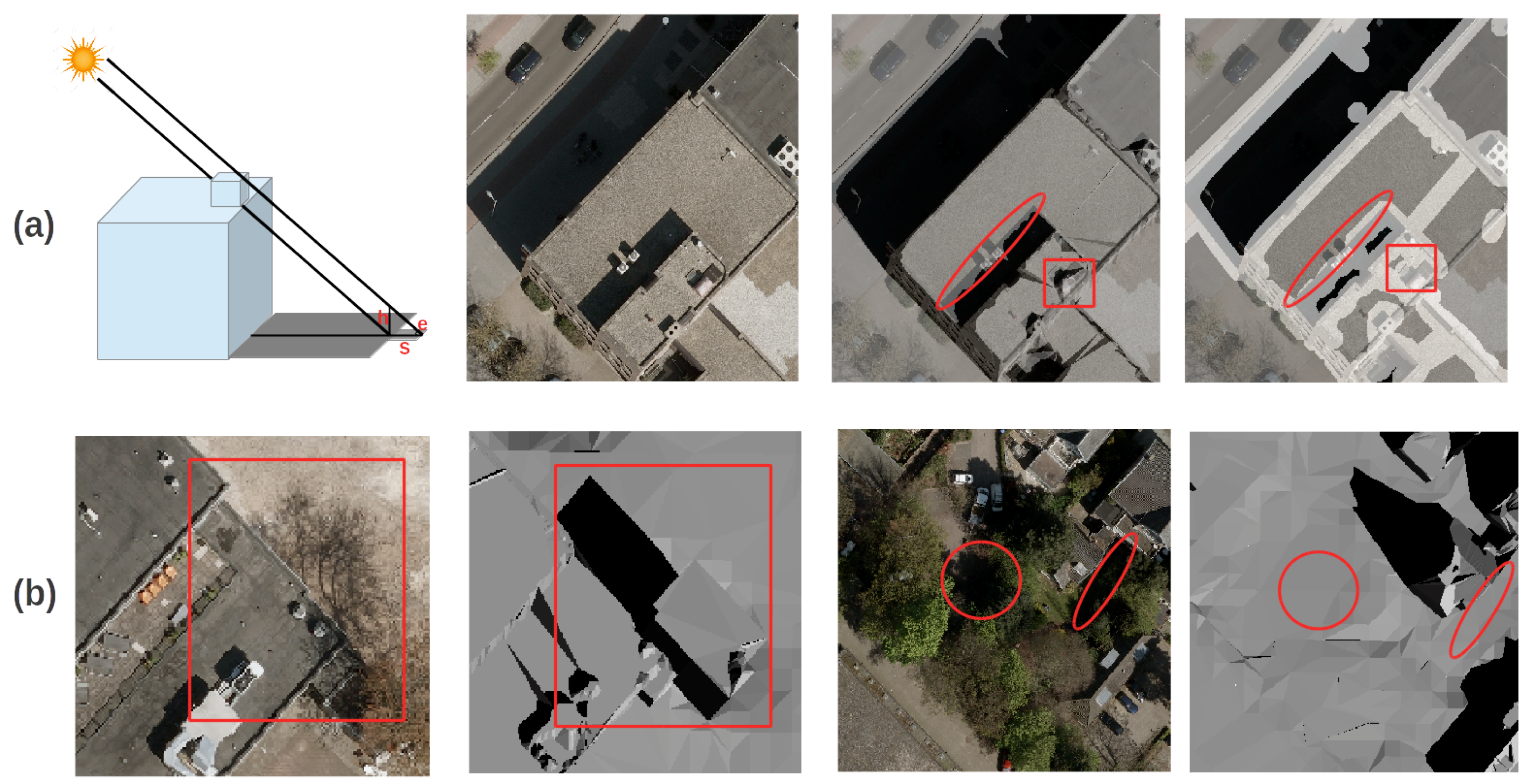
3.1. Shadow Reconstruction Using an Existing 3D Model

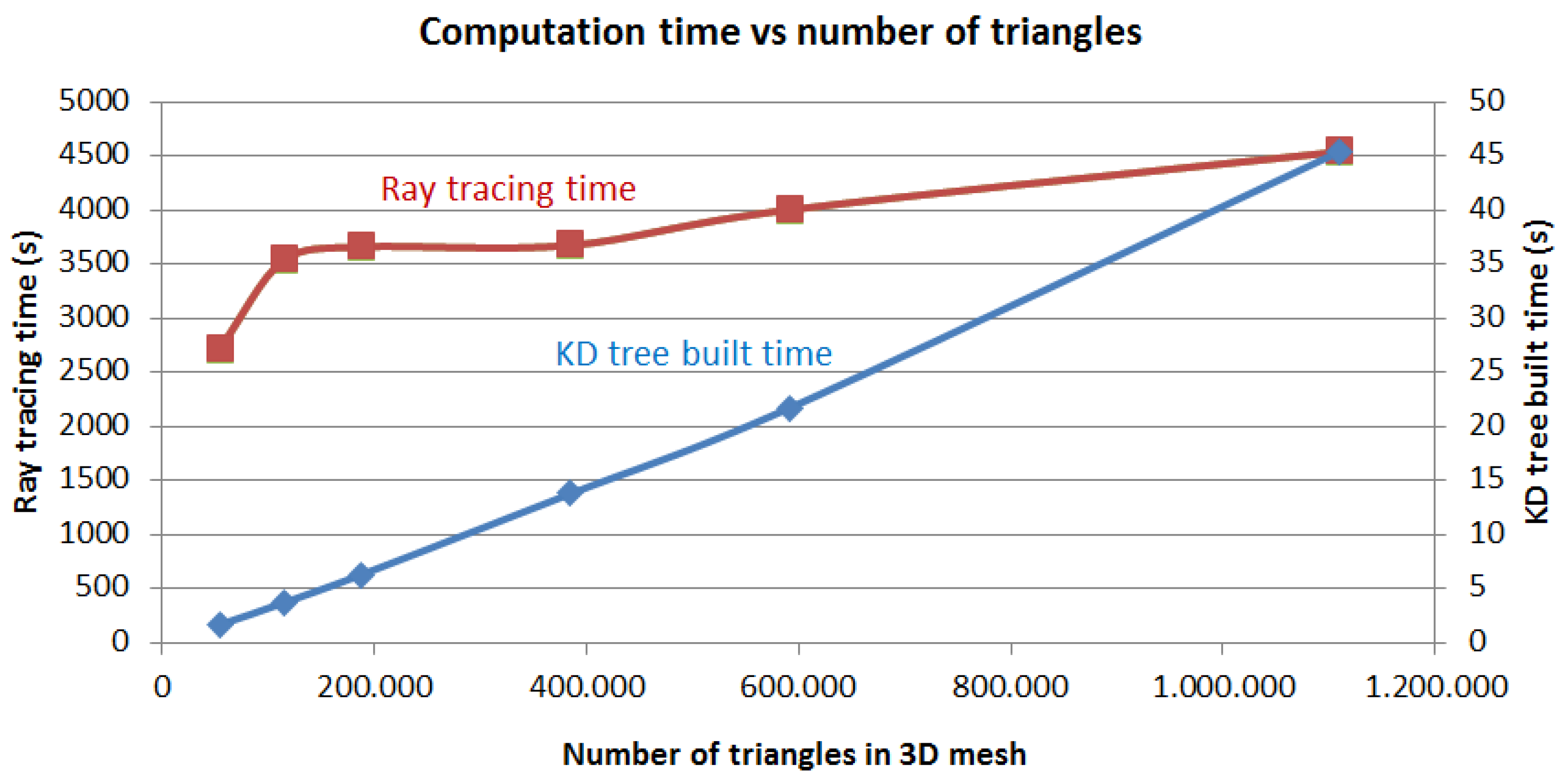
3.1.1. Ray Tracing

We define shadow as that area in VHR images where direct sun light is blocked. However, also areas that do not follow this definition suffer from lower reflectance. Indeed, if the incidence angle between a ray from the sun and the illuminated surface is relatively small, reflectance is reduced. This effect is in principle quantified by means of the so-called Bidirectional Reflectance Distribution Function (BRDF), [22]. In practice however, the notion of BRDF is difficult to use as object reflectance is both material and environment-dependent. These dependencies are difficult to parameterize in an automated way.

Given a 3D model, it is possible to estimate the locations of shadows in a VHR image, according to the definition above, if the sun position and camera interior and exterior orientations are known. The sun position is defined in spherical coordinates by one azimuth and one elevation angle, which can be accurately estimated given the time of acquisition of the VHR image. Camera orientations are accurately estimated by means of bundle adjustment.

Given this information, a computational efficient procedure is to use so-called z-buffering. However, z-buffering is known to cause unwanted aliasing and acne effects. Several approaches, e.g., [23,24], have been designed to mitigate these effects, but implementation is not as straightforward and results are not as accurate as ray tracing [25].

Ray tracing simply generates a viewing ray from each pixel in the image plane through the focal point of the camera to the 3D model. If the first point of intersection between 3D model and ray is in the sun, the pixel is in the sun. Otherwise, the pixel is in the shadow. The disadvantage of this approach is the high computational load. The computational costs of ray tracing are $O(N\ast W\ast H)$, where N represents the number of triangles of a meshed 3D model. The size of the image plane is given as $W\times H$, where W is the number of image columns, and H the number of image rows. Typically, a VHR image consists of millions of pixels, while also a 3D mesh may contain millions of triangles. Therefore, computation is too intensive in practice. Parallelization in CPU and GPU is often applied to reduce computation time. In addition, by incorporating the field of view of the camera in the implementation, the number of triangles considered in the ray tracing can be reduced. However, these two adaptations will only reduce computations linearly, which is not enough to make the overall method computationally feasible.

3.1.2. KD Tree

A KD tree is a space-partitioning data structure. Using a KD tree, search operations are split in two phases. In the first phase, objects, which are in our case the triangles of the 3D mesh, are stored in a search tree of depth k. In the second phase, individual triangle intersection points are determined much faster, given the availability of the search tree. If the triangular space is split into two ($k=2$), a ray first intersects one of two subspaces and next only consider the intersections with triangles in that subspace. If an intersection is found, all triangles in the other subspace can be discarded. To find optimal planes to split the triangles, a local greedy surface area heuristic (SAH) is used under the assumption that rays are equally distributed in space and triangles cover the entire space []. This heuristic minimizes the expected heuristic intersection cost, $C_V\left(p\right)$, of splitting plane p, defined by

$$C_V\left(p\right)={\kappa }_T+{\kappa }_I(\frac{A\left(V_L\right)}{A\left(V_L\right)+A\left(V_R\right)}|T_L|+\frac{A\left(V_R\right)}{A\left(V_L\right)+A\left(V_R\right))}|T_R\left|\right)$$

(1)

Here V indicates the space to be split. In Figure 3 this is the black bounding box containing all triangles. In the figure, splitting plane p is indicated by a red bold line. ${\kappa }_T$ denotes the costs for traversing the two subspaces separated by by splitting plane V, i.e., the rectangles left and right of the red bold line in Figure 3. ${\kappa }_I$ denote the costs for intersecting one triangle, while $A\left(V_L\right)$ and $A\left(V_R\right)$ denote the area of the left and right subspace, respectively. The ratio $\frac{A\left(V_L\right)}{(A\left(V_L\right)+A\left(V_R\right))}$ approximates the percentage of rays going through subspace $V_L$, while $|T_L|$ and $|T_R|$ are the number of triangles in the left and right subspace, respectively.

The equation favors subspaces that are as large as possible but at the same time include as few triangles as possible. The configuration in Figure 3b, shows a case where the split, shown in bold red line, is far from optimal: the left subspace is a little bigger than in Figure 3a, but it contains many more triangles. Every subdivision step minimizes local costs while assuming no subdivision is further performed. The accumulated minimum local costs tend to overestimate the correct total costs as subspaces are in most cases further subdivided. However, in practice, this approximation works well []. The space is subdivided iteratively until $C_V\left(p\right){\kappa }_I·\left|T\right|$.

If a splitting plane slides through the interior of a triangle, compare the blue dashed line in Figure 3b, $|T_L|$ and $|T_R|$ do not change while $C\left(p\right)$ changes in a monotonic way. So optimal planes always occur when the $|T_L|$ and $|T_R|$ are changing, locations indicated by the red dashed lines in the figure. Therefore, the six bounding box planes of each triangle are chosen as candidate planes.

A naive way of plane selection is that for each candidate plane, all left and right triangles are traversed to calculate the SAH cost of that plane, which has a computational load of $O\left(N\right)$. This should be done for all $6·N$ candidate planes so the total computational costs to identify the optimal plane is $O\left(N^2\right)$. Adding the costs for recursive subdivision gives a total cost of approximately 2 times of $O\left(N^2\right)$ for establishing a tree structure. This construction time is not acceptable as it may take hours to apply it in case of 1 million triangles. The naive way is notably expensive due to the costs of classifying triangles for each candidate plane.

In this research, an $O\left(Nlo{g}^{2}N\right)$ approach is adopted instead. A candidate plane is either on the left of, on the right of or passing through a triangle. The number of triangles of each of these types is denoted as $p^{+}$, $p^{-}$ and $p^{|}$ respectively. Once candidate planes are sorted, these numbers can be updated incrementally while sweeping through the sorted list of candidate planes. The full details of the update rules can be found in []. As sorting the candidate planes costs $O\left(NlogN\right)$, while sweeping costs $O\left(N\right)$, the total costs for finding an optimal plane are $O\left(NlogN\right)$. With recursive division, the overall costs are $O\left(Nlo{g}^{2}N\right)$. Consequently, construction time for 1 million triangles can be reduced to minutes in practice []. An even faster algorithm with a cost of $O\left(NlogN\right)$ is obtained by avoiding sorting at each subdivision step, which can be achieved by memorizing the sequence of planes throughout the subdivision (Please note that the triangles and therefore the candidate planes stay the same). The rest is the same as the $O\left(Nlo{g}^{2}N\right)$ approach. However, at the cost of a more complicated implementation, reduction of computation time is only a factor 2 to 3 in practice. In this paper, the $O\left(Nlo{g}^{2}N\right)$ approach is implemented due to its simplicity of implementation. Parallelization of the KD tree construction is not considered for the same reason.

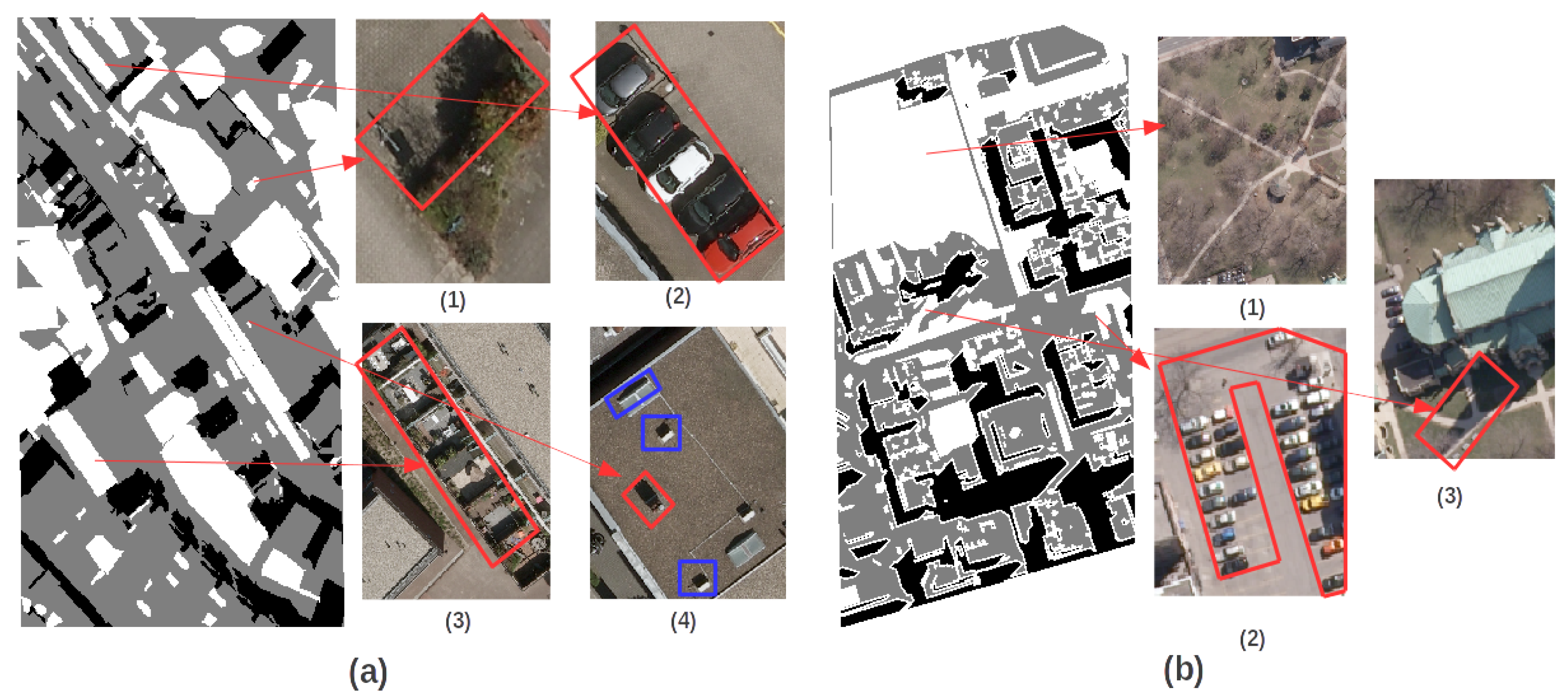
3.2. Adaptive Erosion Filtering

Reconstructing shadows by ray tracing using an existing 3D city model provides sufficient variation in training samples for VHR image classification. However, this procedure also introduces many mislabeled samples. Shadow accuracy near boundaries is affected by misalignments between 3D models and images, and lack of accuracy of the 3D model, especially considering roof details. As the absolute accuracy of both data sources is high, the misalignment is only one or two pixels. These effects are not explicitly considered, as the effects of an inaccurate 3D model are more serious. To mitigate these affects, disk-shaped erosion is applied to remove samples near the boundary of the reconstructed shadows from both shadow and non-shadow training samples. To decide on a good size for the filtering element, we define a simple adaptive rule. The left image in Figure 4a shows that small roof details are able to cast large shadows. The size of such casted shadow depends on the height of the roof detail and the position of the sun. We assume that small details of at most 1 meter height on the roof are artifacts from modeling. The position of the sun is parametrized by two angles: azimuth and elevation. To keep the criterion simple, we only consider elevation. The size, s, of the filter is estimated as

$$s=\frac{h}{tan\left(e\right)\times r},$$

(2)

where r denotes the spatial resolution of the image, h the maximum height of roof details, while e represents the angle of the sun elevation. As similarly roof details may be missing in the 3D model, the same erosion filter is also performed on non-shadow areas. In Figure 4a, the middle two images show an RGB image and reconstructed shadow image. In the square, a small object is poorly reconstructed and some false shadows are constructed. In the circle, a small wall or fence is missing in the 3D model, resulting in some lack of shadows. By applying filters for both shadows and non-shadows, these mislabels are removed. In the right image, the pixels in the white regions are filtered, black pixels are samples for shadows and gray pixels are samples for non-shadows. The selected samples have become more reliable.

However, many training samples are still mislabeled as differences in acquisition time between VHR imagery and 3D model and tree modeling are not incorporated. As shown in the left two images in Figure 4b, the 3D model contains a building which is removed before acquisition of the image. In the right two images, many shadows casted by trees are missing. These mislabels are not trivial and need to be considered when a classification method is selected.

3.3. Classifications from Automatically Selected Samples

A proper classifier should be capable of generalizing the characteristics of complex shadows and at the same time be robust to mislabeling effects. Four common classification approaches, quadratic discriminant analysis (QDA), support vector machine (SVM), K nearest neighbors (KNN) and random forest (RF), are discussed by considering these two requirements. The first method is based on a Gaussian distribution of features. To capture complicated properties of shadows, we use two feature domains: RGB and ratio. The other three classifiers are discriminative classifiers and we confirmed that the ratio feature does not improve classification results.

3.3.1. QDA Classification with Decision Fusion

QDA [27] assumes a Gaussian distribution for each class and fits a quadric surface to train samples to best separate classes. QDA is robust to mislabeling effects as the Gaussian parameters are estimated properly when a large portion of samples is labeled correctly. However, shadows in urban areas are often complicated and certainly not Gaussian distributed. For example, assuming RGB features have a multi-variable Gaussian distribution, property 1, low radiance of shadows, described in Section 1.2, can be generalized. However, property 2, higher hue of shadows, is ignored. A decision fusion approach [28] is adopted to fuse results from QDA on different feature domains, RGB and ratio, to generalize different properties with QDAs [29]. This approach uses fuzzy memberships and assesses the reliability of two classifiers to fuse the result properly. Fuzzy membership describes the confidence of a pixel belonging to a certain class. If two classifiers have different decisions on the class of a pixel, the decision with a higher membership degree is chosen. However, when two classes are not clearly separate in feature space and further confusion is added by mislabeling, a pixel can have high membership degrees for two classes, which means the classifier is not confident in classifying the pixel. Shannon entropy [30] is introduced to measure the reliability of membership degrees as assigned by a classifier. When membership degrees to two classes are high, the reliability is low, and the memberships degrees are weighted by the reliability for decision fusion. This approach improves the QDA classifier to have more power to capture complex shadow properties. However, the ratio feature is designed to enlarge difference between shadows and non-shadows. The mixture problem is less serious, so this decision fusion approach may rely more on the decisions from ratio domain. Furthermore, the properties 3 and 4 from Section 1.2 are not considered in this method.

3.3.2. Support Vector Machine

SVMs have been successfully used for shadow classification [8,13]. SVMs aim to fit an optimal hyperplane to the training samples to maximize the margins between the separating plane and the closest training samples (support vectors) [27]. If the classes are not separable or the separation surface is nonlinear, the input data are mapped by kernel functions to a higher dimensional feature space where it is possible to find an optimal hyperplane. This approach avoids assumptions on the data distribution and is effective in deriving complicated nonlinear hypersurfaces to separate classes. However, mislabeled samples near the separation boundary will increase the complexity of SVMs’ boundaries and result in an overfitting problem [31]. A soft-margin, a regularization term to penalize samples located at the wrong side of the separation hyperplane, can help to increase the robustness of SVMs to mislabeling. When the weight of the regularization term is set too large, SVMs loss the ability to find accurate separation boundaries.

3.3.3. K Nearest Neighbors

KNN is also a non-parametric classifier. They do not use training samples to estimate a model, but they store training samples to decide which class should be assigned to an unseen sample. An instance is classified by majority voting from k nearest neighbors, which means the class for the instance depends on the most common class among its k nearest training samples. This approach is capable of capturing complicated data distributions if an optimal k is selected. A larger k can suppress noise and smoothen separation boundaries; however, it may affect the ability to capture detailed properties from the training samples. Okamoto and Nobuhiro (1997) [32] showed that the robustness of KNN to mislabeled samples is dependent on an optimal selection of k. k should increase as the ratio of mislabeled samples increases. So, the optimal value of k is case-dependent and difficult to set adaptively. Cross-validation is widely used for choosing the optimal k, but an accurate validation dataset should be manually selected.

3.3.4. Random Forest

Ensemble learning consists of a collection of classifiers and has been applied successfully in remote sensing. The most well-known classifiers are AdaBoost [33] and RF [34]. AdaBoost is an ensemble of classifiers that reweighs samples by giving incorrect classified samples more weight for the next classifier. Every classifier gets a weight based on its classification accuracy and a weighted majority voting determines the final class assigned to test samples. AdaBoost tends to avoid overfitting when mislabels are trivial [35] and generally has good classification performance. However, if mislabels are introduced, the reweighting mechanism would emphasize to classify the mislabeled sample in the next tree, which results in a serious overfitting problem. RF, instead, adopts a bagging mechanism by randomly selecting a subset of samples and features by replacement for training each classifier. Breiman (2001) [36] demonstrates that RF has a classification accuracy that is comparable to AdaBoost on a test consisting of 20 datasets. Moreover, the assembly of decision trees by bagging guarantees that RF is robust to noises [36]. It is tested to outperform AdaBoost significantly when 5% of mislabeled training samples are introduced [36].

In building each decision tree, the choice of attribute selection and a pruning method are important [37]. The Gini index [38] is chosen to measure impurity of separated classes when an attribute value is chosen to split a tree. An attribute with lowest impurity of separation is chosen as the optimal value to split the tree. Choosing a pruning method affects the performance of decision trees due to overfitting effects. However, trees in RF do not need to be pruned. Breiman (2001) [36] demonstrate that as the number of trees grows, the generalization error of classifying unseen data always converges and overfitting is not a problem. This simplifies the setup of the hyper-parameters in RFs. As in our research only three features are used, all of them are used for each tree. As our number of training samples is very large, we randomly choose different subsets of 10,000 samples for each class for constructing 100 trees. In this way, constructing 100 trees is computationally efficient and trees are less correlated which contributes a small generalization error even with fewer trees. If more trees are selected, no obvious improvement is expected.

3.4. Evaluation of Classification

Pixel-based classification in VHR images often has a salt and pepper noise problem. First, an erosion morphological filter is applied and next a dilation morphological filter is applied to correct unwanted erosion effects. The size of the dilation morphological filter is larger than erosion filter due to penumbra effects. The equation for calculating penumbra areas is provided in [39] with respect to the height of object, h and elevation angle of the sun, e, as follows:

$$w=h(\frac{1}{tan(e-\frac{ϵ}{2})})-\frac{1}{tan(e+\frac{ϵ}{2})}))$$

(3)

where w is the penumbra width and $ϵ$ is the angular width of the sun which is ${0.5}^{\circ }$. As we filter the boundary pixels from reconstructed shadows to avoid issues caused by misalignment between model and image, and low quality of model near rooftops, pixels in the penumbra areas are not included in the training samples. These pixels are more likely classified into non-shadows as they are brighter. If shadows are used to estimate building height or for change detection, the estimated building height will be too low and false alarms near shadow boundaries will result in false change detection. Therefore, the detected shadows should be dilated with size of w. In this study, the border between shadow and non-shadow pixels in a mixed penumbra area was visually chosen in the middle of the areas for creating test dataset. Therefore, we decided to dilate with a half size.

The test dataset is drawn manually by drawing polygons in QGIS. The resulting vector file is then converted to reference images, shown in Figure 5. Several criteria have been designed to create labels for the test dataset: (1) Shadow pixels are labeled based on whether it was blocked from sunlight even they have high reflectance. In penumbra areas, the boundary between shadow and non-shadow is visually chosen in the middle of the areas. (2) Shading effects are not considered in manual labeling. If the incidence angle is small, roof pixels may look similar to shadow pixels. Still, we label them as non-shadows as they are not blocked from sunlight. (3) Only shadows caused by buildings are selected, while shadows from vegetation, cars and objects in the garden are excluded. The building shadows for Amersfoort are manually selected. As the 3D model for Toronto is manually created, the building shadows are selected from the reconstructed shadows. Shadow boundary parts are excluded from the image to reduce the effects of misalignment between images and 3D model, and inaccurate details in rooftops. Wrong shadows due to a few model errors are also excluded as shown in Figure 5b (3). As shown in Figure 5a, labeling these cases manually is time-consuming. If shadows are used to help the detection of different objects, shadows are notably useful for building detection. Vegetation and cars can be detected accurately from color information and objects in the gardens are not interesting. These shadows are excluded from the test dataset by roughly draw bounding polygons. (4) Shadows from small details, less than 1 m by 1 m, on the roof are often not necessary to detect. As they are too many to be excluded, these shadows are included in non-shadows as shown in Figure 5a (4). Accordingly, shadows from these details which are detected from images should be converted to non-shadows.

All classification methods are trained by samples labeled from the reconstructed shadow image and are consecutively applied to classify the test dataset. The results are compared with manual labels to derive the evaluation of their performance. To compare effects of different methods on shadow detection qualitatively, four metrics are selected: producer’s accuracy($\tau$), user’s accuracy($\sigma$), overall accuracy(OA) and kappa coefficient (KC).

$$\tau =\frac{TP}{TP+FN},\sigma =\frac{TP}{TP+FP}$$

(4)

$$OA=\frac{TP+TN}{N},KC=\frac{OA-p_e}{1-p_e},p_e=\frac{(TP+FP)\times (TP+FN)+(FN+TN)\times (FP+TN)}{N\times N}$$

(5)

N presents the total number of pixels. TP, FP, and FN denote the true positives, false positives and false negatives respectively. The producer’s accuracy describes how accurately a method detects shadows. In other word, it quantifies the completeness of shadow detection. User’s accuracy describes the correctness of shadow detection. Overall accuracy refers to the percentage of shadow and non-shadows pixels correctly detected. KC is a robust measurement of how well a classifier works by taking into account how well a classifier would work simply by chance. $p_e$ denotes the accuracy of detection by chance.

4. Experiments and Comparisons

Experiments are applied to two city areas in Amersfoort and Toronto. The experiments consist of two steps: shadow reconstruction to obtain free-training samples and classification after training with these samples. The purpose of the first step is to show how efficient ray tracing is for shadow reconstruction in large 3D models. In the second step, the Amersfoort and Toronto dataset are tested with the four methods described in Section 3.3. By testing comparative methods in different environments, the robustness of each method is tested with respect to its capability of capturing complicated shadows properties and mislabeling effects.

4.1. Feasibility of Shadow Reconstruction for Free-Training Samples

Ray tracing with KD tree acceleration for shadow reconstruction was implemented in C++ on a HP laptop with 8 GB ram and quadcore processor. The KD tree construction is not parallelized, but ray tracing is parallelized in CPU. As described in Section 3.3.1, shadow ray tracing requires camera parameters and the sun position. The camera parameters are obtained from their bundle adjustment files. For the Amersfoort data, from the acquisition time of the image, an accurate azimuth and elevation angle of sun position are easy to obtain. They are ${44.58}^{\circ }$ and ${140.41}^{\circ }$ respectively. The Toronto data do not provide acquisition time, but the sun position can be estimated. One obvious building roof corner in the 3D model and its shadow pixel in the image are found. From the shadow pixel, a camera ray is generated to find its intersection with the model. The intersection shows the shadow point in the 3D model casted by the roof corner. The line between the shadow point and roof corner is actually a sun ray. The 3D line can be transformed into spherical coordinate system. Therefore, the azimuth and elevation of Toronto data are estimated at ${49.93}^{\circ }$ and ${133.13}^{\circ }$ respectively. The shadow images created have the same size as the aerial images: 11,310*17,310 and 7500*11,500 for Amersfoort and Toronto, respectively. The time for building a KD tree is 21.27 s and 1.14 s respectively as the number of triangles in the Amersfoort model is 10 times higher than in the Toronto model. The ray-tracing time is 3840 s and 281 s, respectively. The number of triangles and image size is larger in Amersfoort, but the most important factor is the structure of 3D models in the view of the camera. As shown in Figure 6, fewer camera rays from Toronto image pixels intersect with the 3D model resulting in a large number of white pixels. Due to the KD tree structure, the rays from most of the white pixels only need one intersection test with the bounding box of the model indicated the 2D red box. The reconstructed shadow images are shown in Figure 6, while the shadow images in the area of interest are displayed in Figure 2c.

We conducted an experiment to subsample the point cloud of Amersfoort at different size and make different triangular meshes while preserving the structure of the 3D model for ray tracing. These models are applied to test the efficiency of building KD trees and ray tracing relative to the number of triangles. The number of triangles of five simulated models varies from 54,000 to 1,1100,000. In each ray-tracing experiment, the number of white pixels is the same while the number of triangles is changed uniformly. The result is shown in Figure 7. The time for building a KD tree scales nearly linear with the number of triangles, which confirms the computation complexity of $O\left(Nlo{g}^{2}N\right)$. As N becomes larger, $lo{g}^{2}N$ is hardly noticeable. Even from 54 k to 1 million, the $lo{g}^{2}N$ term only contributes by a factor of $\frac{lo{g}^2\left(1million\right)}{lo{g}^2\left(54k\right)}=1.6$. Therefore, the time is almost linear in N. Due to the large number of rays from pixels, around 200 million in our experiment, ray tracing needs 45 mins with 54 k triangles. However, when the number of triangles increases a factor of 20, from 54 k to 1.11 million, the processing time only increases by a factor of 1.6. Using a KD tree structure, the time of ray tracing is almost increasing logarithmically with the number of triangles. To conclude, the experiment shows the feasibility of the effective KD tree construction and ray tracing and demonstrates that using a KD tree makes it possible to reconstruct shadows from a 3D model, even in case of large datasets.

4.2. Method Comparison for Classification from Free-Training Samples

The classification methods used in the paper are implemented in MATLAB using the precoded classifiers. The script for comparative analysis is also written in MATLAB. The samples for shadow reconstruction are unbalanced. Shadows occur less than non-shadows. Equal numbers of samples, 10,000, are randomly selected for each class for classification. Tests showed that adding more samples did not improve results as the randomly selected samples are representative enough for both data. Only RF randomly selects free-training samples from 1 million samples for each decision tree. This step increases the variety of decision trees but does not increase the computations. Parameters chosen for the different methods are the same for both datasets to test the applicability of the methods. QDA fusion is free of any input parameters. For SVMs, the weight for the regularization term is 0.2 for training samples with mislabels. The weight is set to 0 for Toronto as only a limited mislabels is present. For KNN, k is chosen to 11 to have robustness to mislabel. For RF classification, all three features are used in every tree and 100 trees are selected as the performance does not significantly improve by adding more trees.

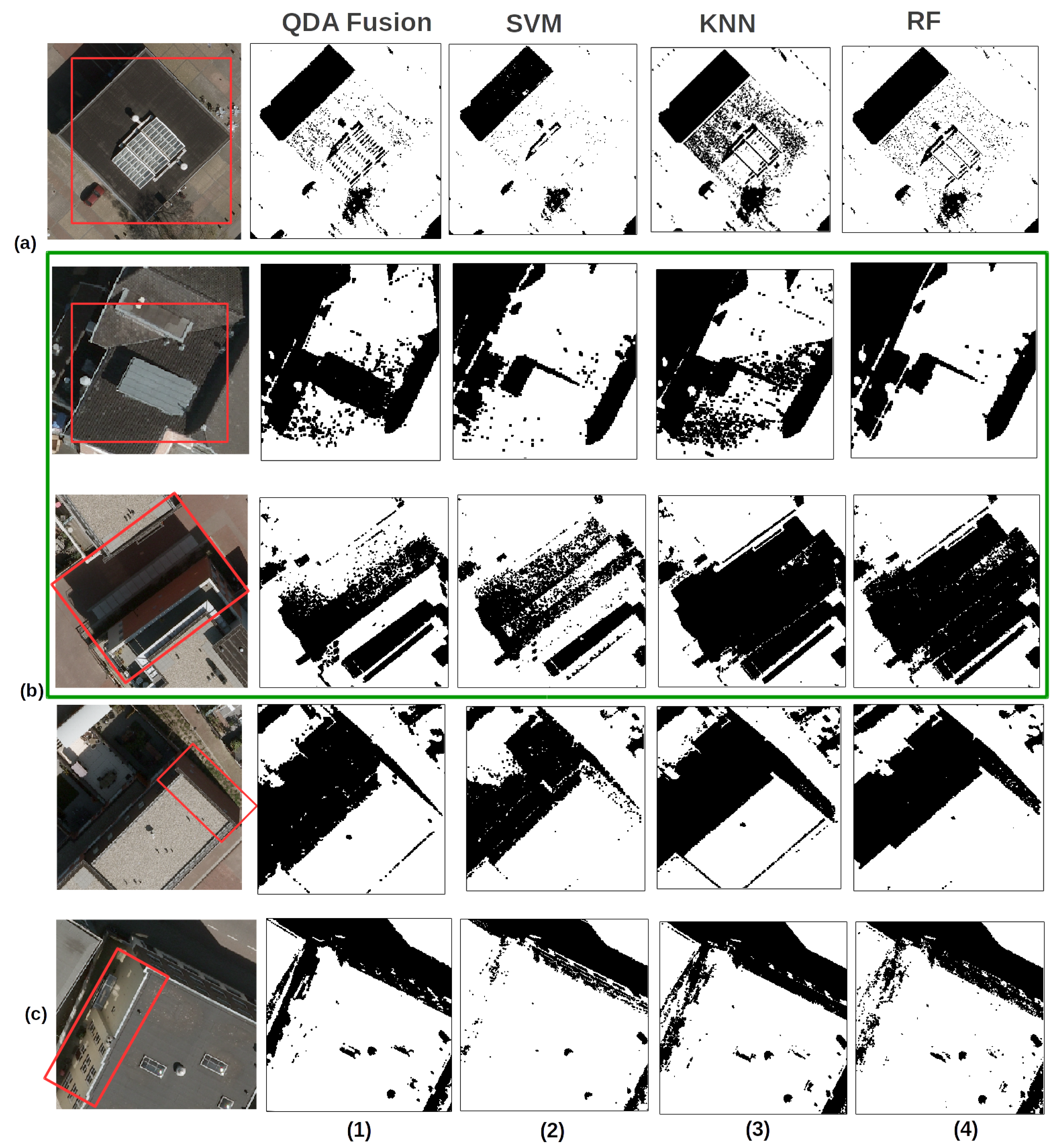
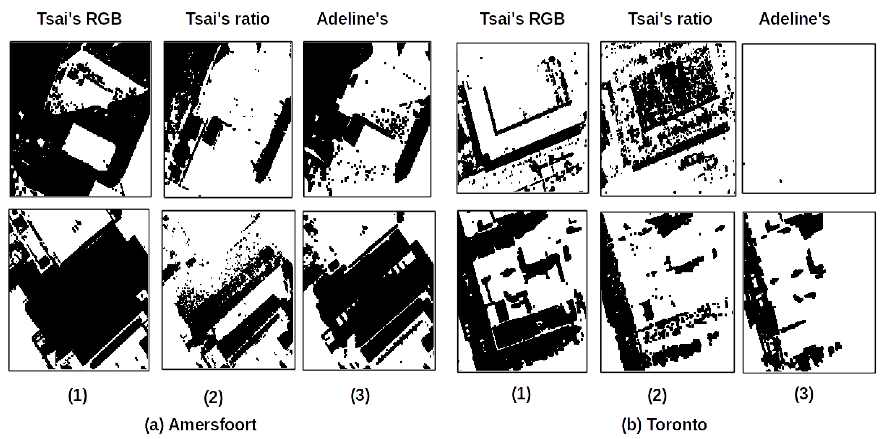
4.2.1. Shadow Classification Results for Amersfoort

Before classification, according to Section 3.2 an adaptive disk-shaped erosion is applied to remove the boundary parts of shadows and non-shadows. With its 3.5 cm spatial resolution, the size of the filter is set at 30 according to Equation (2) in Section 3.2. After each classification, according to Section 3.4, an erosion filter is applied to mitigate the salt and pepper noise problem of classification results and a dilation filter is then applied to correct unwanted erosion effects and compensate for the effects of mixed pixels in penumbra regions. An erosion filter with a size of 1 is applied to remove noise from detection. According to Equation (4) in Section 3.4, if we assume the height of buildings at 10 m, a half of the penumbra width is 8 cm. Therefore, a dilation filter with a size of 3 is applied to reconstruct the erosion effects and reduce penumbra effects.

Table 1. Comparative results for shadow detection in Amersfoort.

Method	$\mathit{\tau }\%$	$\mathit{\sigma }\%$	OA %	KC
QDA Fusion	89.92	95.80	93.45	0.87
SVM	84.66	98.88	92.08	0.84
KNN	95.61	95.65	95.72	0.91
RF	93.92	96.12	95.38	0.92
Tsai’s RGB	99.12	70.88	80.51	0.62
Tsai’s ratio	82.34	91.46	88.18	0.76
Adeline’s	90.95	97.53	94.20	0.88

shows that KNN and RF gives similar and outperform the other classifiers. The producer’s accuracies ($\tau$) are $95.61\%$ and $93.92$. The user’s accuracies ($\sigma$) are 95.65% and 96.12% respectively. This indicates that the two methods obtain a good completeness of shadow detection while keeping a high correctness. Problematic areas as shown in Figure 8a,b, like dark roofs in the sun and reddish objects in the shadow are well distinguished by RF. As shown in Figure 8a, KNN is worse in classifying dark roofs. This explains why its $\sigma$ (correctness) is a bit lower. In Figure 8b, both perform well on detecting shadows in reddish objects. The high overall accuracy of more than 95% and KC around $0.91$ for both methods show the capability of both methods to generalize the complicated properties of (non-)shadows from mislabeled samples. The complete result of shadow detection from RF is shown in the left image of Figure 2d.

The QDA fusion method has a relatively low completeness $\tau$ ($89.92\%$). It fails to detect reddish objects in the shadow correctly with two cases as shown Figure 8b. In the upper case, the reddish road pixels near the reddish facade are darker, so they are correctly detected as shadows. However, when reddish road pixels far away from the facade become brighter, they are wrongly classified. The same happens with reddish facades in the shadow in two buildings as pixels receive more reflected light. In the RGB domain, dark pixels could be assigned to shadows, while in the ratio domain, the pixels with reddish color could be assigned to non-shadows. The QDA fusion approach makes a decision based on two variables: confidence and reliability of each result. When the reddish pixels become lighter, the confidence that these pixels belong to shadows is less, while more reddish reflectance gives more confidence that they belong to non-shadow in the ratio domain. Therefore, the decision fusion approach is still not capable of capturing complicated shadow properties. Still QDA fusion has better results than SVM due to its robustness to mislabels. The ability of SVM to find good separation in complicated areas is largely deteriorated by mislabels. The regularization term is not really helpful to deal with the mislabels as SVMs cannot distinguish the pixels which define complicated separation boundaries from pixels which are mislabeled. This results in the lowest $\tau$ ($84.66\%$) and highest $\sigma$ ($98.88\%$). It indicates that SVMs are not robust to mislabeling. In Figure 8c, four methods show low detection accuracy on the high reflectance facade with high RGB values.

Two property methods by histogram thresholding from Tsai [9] and Adeline et al. [7] are selected. The main difference of these two methods is their thresholding approach. Tsai uses Otsu’s method [11], while Adeline et al. set the threshold at the first valley of the histogram which gives the best shadow detection performance in their comparative study. Tsai’s method is applied to two feature domains RGB (Tsai’s RGB) and ratio (Tsai’s ration) respectively, while Adeline’s method is applied to intensity. As shadows in Amersfoort are strongly affected by reflection from environment and materials, the histogram is noisy. The value at the first valley is certainly not the best threshold and often much lower than the best threshold. We smooth the histogram by Savitzky-Golay smoothing [40] and set a constraint that the threshold found should not be lower than 25. As the property methods perform well only for a bimodal histogram, the image is split into small patches, in which bimodal behavior is more likely to appear. As shown in Table 1, Tsai’s methods on RGB and ratio domain tend to over- and miss-detect shadows, respectively. In Figure 9a (1) and (2), Tsai’s methods cannot distinguish dark roofs in the sun and reddish street in the shadow properly. Both have the lowest OA and KC. Adeline’s method shows a better result than Tsai’s method. In Figure 9a (3), Adeline’s method shows a good result in classifying these two cases. Still, the completeness and KC are 3% and 0.04 lower than RF, respectively. More importantly, thresholding at the first valley of a histogram is not robust in case of complicated shadows and tends to miss-detect shadows. This effect is more obvious in the Toronto experiment.

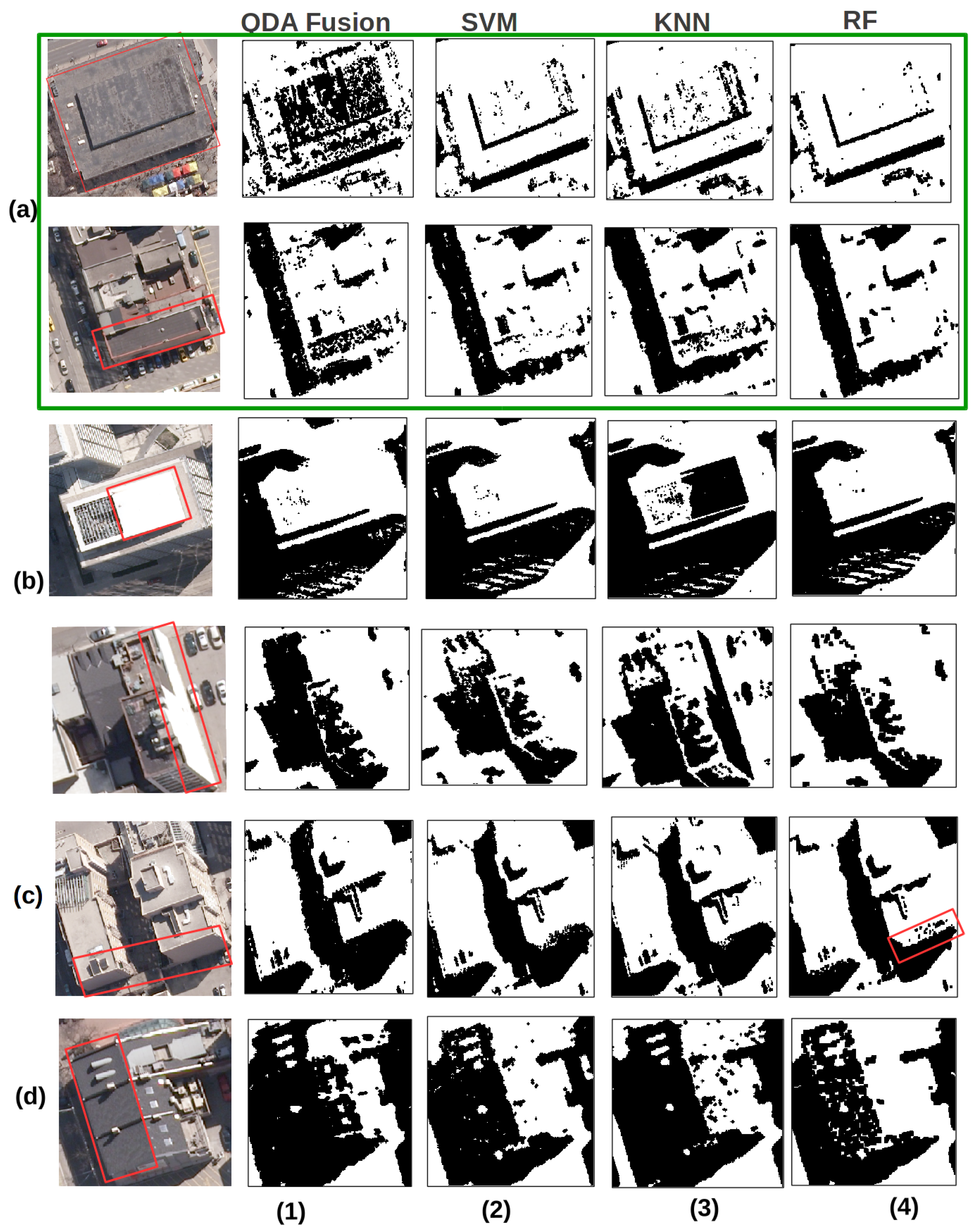
4.2.2. Shadow Classification Results for Toronto

The same disk-shaped erosion filter is applied to remove the boundary parts of shadows and non-shadows. As the spatial resolution of pixels is 15 cm, the size of the filter is set at 6 according to Equation (2). After classification, an erosion filter with size of 1 is applied to remove noise. According to Equation (4), if we assume the height of buildings in Toronto downtown to be 40 m, the half of penumbra width is 28 cm. So, a dilation filter with size of 3 is applied to reconstruct the erosion and reduce the effects of mixed pixel in the penumbra areas. The classification results are shown in

Table 2. Comparative results for shadow detection in Toronto.

Methods	$\mathit{\tau }\%$	$\mathit{\sigma }\%$	OA %	KC
QDA Fusion	94.99	88.82	95.16	0.88
SVM	94.20	93.98	96.69	0.92
KNN	97.69	88.63	95.85	0.90
RF	97.34	91.05	96.59	0.92
Tsai’s RGB	98.50	83.41	92.87	0.85
Tsai’s ratio	95.60	82.75	93.20	0.84
Adeline’s	80.48	92.81	92.55	0.81

.

In this experiment, in the training set, mislabels are limited as the building models are accurate and trees are sparse and limited. All methods have good completeness with producer’s accuracy ($\tau$) values of more than 94 %. However, QDA fusion has a relatively low user’s accuracy ($\sigma$), 88.82%. QDA fusion makes a good detection on the bright shadows on the facade in Figure 10c; however, the dark roofs of two buildings indicated in the red boxes are seriously misclassified as shadows in Figure 10a. It confirms that QDA fusion is still not good enough to capture complicate shadows. KNN has the highest completeness of shadow detection at $\tau$ value of 97.69 %. However, its correctness of shadow detection has a much lower value for Amersfoort and it has a lowest $\sigma$ (88.63 %) value. KNN has a little worse classification on the dark objects as shown in Figure 10a, but a more serious problem is shown in Figure 10b. KNN has difficulties in classifying very bright white walls and roofs. Although a few white pixels are labeled as shadows in the reconstructed shadow image, the percentage of white pixels in shadow training samples is higher than in the non-shadow training samples. As we select the same amount of shadow and non-shadow samples, more white pixels in the shadow training samples are selected. This problem can be solved by increasing the number of nearest neighbors, K. However, it will also smoothen the boundary between shadow and non-shadows.

SVM and RF have competitive results with balanced high $\tau$ and $\sigma$ and a higher overall accuracy of more than 96 % and kappa coefficient around 0.92. The complete shadow detection result by RF is shown in the right image of Figure 2d. The good performance of SVM confirms that SVM is applied to shadow detection in literature in case of almost perfect training data. In Figure 10c, the indicated facade in the shadow appears bright due to reflection and its material. Consequently, the pixels are easily mixed with dark objects in the sun from Figure 10a. RF has less accurate detection in Figure 10c, but most of shadows on the facade are captured. Both methods make a good trade off in balancing these mixed cases in Figure 10a,c. This confirms that both SVM and RF are capable of capturing complex shadow properties. Figure 10d shows that the roof indicated in the red box is a bit darker due to shading effects. The incidence angle between sun ray and the roof is larger than its neighboring roof in the same building. With less reflectance, all four methods make a wrong classification. The same effect also happens in Figure 10b as indicated in the green box. These effects could be solved by compensating for the shading effects by taking the incident angle from ray tracing into account. However, how much to be compensated for is strongly related to material property. If the neighboring roof could be identified to be made of the same materials, the compensation could be estimated. However, this would involve segmentation or classification steps, which is therefore not considered in this research. SVM is expected to become more serious when the ratio of mislabeled training samples increases. This effect is obvious in the Amersfoort dataset and will be further tested in the next section by simulating mislabeled samples in the training data.

Compared to Tsai’s and Adeline’s methods, the supervised approaches perform all better. Tsai’s method tends to over-detect shadows as they have 98.5% and 95.60% completeness ($\tau$) respectively, but low correctness with 83.41% and 82.75% ($\sigma$) respectively. The low correctness of shadow detection can be seen from Figure 9b (1) and (2). Tsai’s methods have difficulties to detect dark roofs in the sun correctly. Adeline’s methods tend to miss-detect shadows as the threshold at the location of the first valley is often lower than the best threshold. Therefore, the producer’s accuracy is lowest at 80.47%, while the users’ accuracy is high at 92.81% of $\sigma$. The serious effect is shown obviously in Figure 9b (3). A large portion of shadows is miss-detected from two cases. In the lower case, the shadow result is combined from two patches. In the right half of the image, the threshold found is much lower than the best, so all shadows are mis-detected. The different results from adjacent patches also shows that Adeline’s method is not robust due to complexed environment.

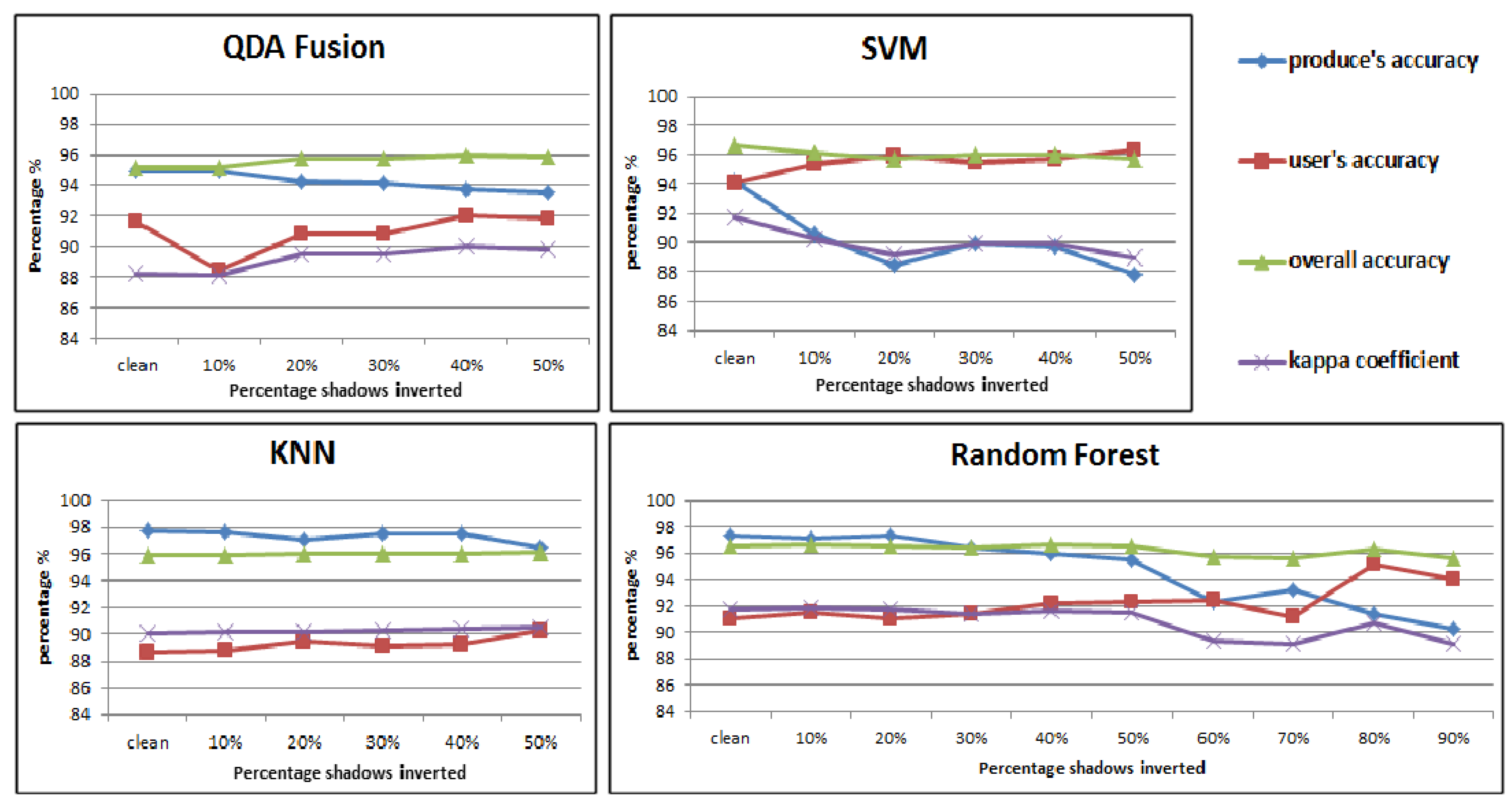
4.2.3. Mislabeling Simulation on Toronto Dataset

To test how robust different methods are to the effect of mislabeling in case of Toronto dataset and whether results are consistent to the Amersfoort case, different levels of mislabeling are applied to the non-shadow training samples in Toronto. The implementation is set as follows: First, shadow pixels are segmented using connected component labeling. Then randomly selected segments are inverted to non-shadows. This approach simulates a scenario where buildings did not exist in the building model but were newly built before the images were taken. Five levels of mislabeling are simulated by inverting 10% to 50% of original shadows in steps of $10\%$. The results are shown in Figure 11. The results from the clean dataset shown in Section 4.2.2 are included for comparison.

In general, the producer’s accuracy decreases, and the user’s accuracy increases when the level of mislabeling increases in the non-shadow samples. When the non-shadow training samples are contaminated by many shadow pixels, fewer shadow pixels are detected but the detected shadows have higher correctness. As shown in Figure 10, QDA fusion and KNN are more robust to mislabeling even with a high ratio of mislabels. Interesting is that the results of QDA fusion are slightly increasing when the mislabeling level increases. QDA fusion tends to over-detect shadows with low correctness without mislabeling simulation. When more shadows samples are mislabeled as non-shadows, it reduces this tendency and the results improve. KNN shows its highest robustness to mislabeling. The reason is that a large K, 11, is used in the experiment. The producer’s accuracy of the SVM drops quickly when mislabels begin to increase. It confirms the results from the Amersfoort experiment, which indicates that SVM has overfitting problems when training samples have been mislabeled. Another interesting finding is that the performance stabilizes when 30% shadows are inverted. RF remains robust and has highest OA (more than 96%) and KC (around 0.92) when the percentage of inverted shadows is between 10% and 50%. To evaluate complete performance of RF to mislabeling, we simulate the percentage of inverted shadows until 90%. The producer’s accuracy has a trend to decrease started from 60% of shadows are inverted. In particular, the producer’s accuracy decreases dramatically from 95.5% to 92% once 60% of shadows are inverted; however, the user’s accuracy stays the same. This indicates that RF starts to be affected by mislabeling. An interesting finding is that after 70% shadows have been inverted, the user’s accuracy starts to increase, which causes KC to increase. This means that mislabeled samples help to detect dark objects in sun which are seriously mixed by shadows. Due to its unstable performance, random forest is only recommended when an urban area has not changed dramatically. It is also a reasonable assumption that if an urban area has changed dramatically, the 3D model is better to be discarded.

5. Conclusions

3D city models are often available presently; however, they are quickly outdated as well. VHR images with an annual updating rate are useful for creating up-to-date 3D city models or detecting changes in existing models. As urban areas in general do not change dramatically, an existing 3D city model in return can provide a lot of correct information that can be exploited to interpret newer images. This paper uses an existing 3D model to reconstruct shadows in images for providing a large variety of training samples to detect shadows in the same images. Free-training samples enable the robustness of the application to large and various areas. The focus in this paper is on two main aspects. First, the feasibility of accurate shadow reconstruction in large 3D models by automatically generating training data and second, the robustness of shadow detection in case of complicated shadows and mislabeling. A ray-tracing approach combined with an effective KD tree construction algorithm is designed. By testing the algorithm to different sizes of 3D models, experiments show that building a KD tree is efficient as the computation time almost scales linearly with the number of triangles. However, ray tracing is more time-intensive, but the time is almost linear with the logarithm of the number of triangles. Even though the time has a high basis, time increases much less when the number of triangles increases. As ray tracing is highly parallelizable, the algorithm can be run directly in the server by using more CPUs to make it faster. With respect to the KD tree built and ray-tracing time, the algorithm is applicable to an even larger model than our experiments. A comparative study on four classification methods is performed to choose one with two criteria: capability of generalizing the complicated properties of shadows and robustness to a certain level of mislabeling. The experiments using Amersfoort and Toronto data use the same hyper-parameters for the four methods. The QDA fusion is robust to mislabeling but has difficulties in capturing complicated shadow properties. KNN is also robust to mislabeling, and the performance of classification is good in Amersfoort, but not in Toronto. Thus, the capability of capturing complicated boundaries is case-dependent. SVM is confirmed in Toronto with a power in classifying complicated shadows as shown in many studies [8,12,13]; however, it is strongly affected by mislabels. RF outperforms the other three methods when mislabels are not significant in both datasets. Only when more than 50% of shadows in Toronto are mislabeled as non-shadows does performance drop. Good shadow and non-shadow detection are both important to applications, such as building detection, height estimation, building change detection or shadow compensation during semantic classification. As urban areas often do not change dramatically, RF showed good results in detecting both shadow and non-shadow using free-training samples. The hyper-parameters for RF are easy to set and tested robustly to different datasets. Compared to two property approaches, Tsai’s [9] and Adeline’s methods [7], RF is better than all the results from both methods when applied to Amersfoort and Toronto.

As the accuracy of shadows contributes directly to quality of different applications, there are two recommendations: (1) improve shadow detection by including texture information and shading effects; and (2) use the linkage between shadows and buildings to improve shadow and building detection. Deep learning is booming in image recognition due to its ability to learn informative features. Convolutional neural networks are more powerful in extracting texture features by learning from training samples than handcrafted features. Shading effects also affect shadow detection, especially in the Toronto dataset. As textural information of building roofs is diverse, building detection or change detection from VHR images is difficult. Even when shadows are not perfect, the linkage between shadow and buildings can be used to improve building detection [6]. For building change detection by using shadows, a similar strategy can be applied.

References

1. Haala, N.; Kada, M. An update on automatic 3D building reconstruction. ISPRS J. Photogramm. Remote Sens. 2010, 65, 570–580. [Google Scholar] [CrossRef]
2. Vosselman, G.; Dijkman, S. 3D building model reconstruction from point clouds and ground plans. Int. Arch. Photogramm. Remote Sens. Spat. Inf. Sci. 2001, 34, 37–44. [Google Scholar]
3. Hirschmuller, H. Stereo processing by semiglobal matching and mutual information. IEEE Trans. Pattern Anal. Mach. Intell. 2008, 30, 328–341. [Google Scholar] [CrossRef] [PubMed]
4. Hartley, R.; Zisserman, A. Multiple View Geometry in Computer Vision; Cambridge University Press: Cambridge, UK, 2003. [Google Scholar]
5. Zlatanova, S.; Holweg, D. 3D Geo-information in emergency response: A framework. In Proceedings of the Fourth International Symposium on Mobile Mapping Technology, Kunming, China, 29–31 March 2004; pp. 29–31. [Google Scholar]
6. Ok, A.O. Automated detection of buildings from single VHR multispectral images using shadow information and graph cuts. ISPRS J. Photogramm. Remote Sens. 2013, 86, 21–40. [Google Scholar] [CrossRef]
7. Adeline, K.; Chen, M.; Briottet, X.; Pang, S.; Paparoditis, N. Shadow detection in very high spatial resolution aerial images: A comparative study. ISPRS J. Photogramm. Remote Sens. 2013, 80, 21–38. [Google Scholar] [CrossRef]
8. Lorenzi, L.; Melgani, F.; Mercier, G. A complete processing chain for shadow detection and reconstruction in VHR images. IEEE Trans. Geosci. Remote Sens. 2012, 50, 3440–3452. [Google Scholar] [CrossRef]
9. Tsai, V.J. A comparative study on shadow compensation of color aerial images in invariant color models. IEEE Trans. Geosci. Remote Sens. 2006, 44, 1661–1671. [Google Scholar] [CrossRef]
10. Chung, K.L.; Lin, Y.R.; Huang, Y.H. Efficient shadow detection of color aerial images based on successive thresholding scheme. IEEE Trans. Geosci. Remote Sens. 2009, 47, 671–682. [Google Scholar] [CrossRef]
11. Otsu, N. A threshold selection method from gray-level histograms. Automatica 1975, 11, 23–27. [Google Scholar] [CrossRef]
12. Arbel, E.; Hel-Or, H. Shadow removal using intensity surfaces and texture anchor points. IEEE Trans. Pattern Anal. Mach. Intell. 2011, 33, 1202–1216. [Google Scholar] [CrossRef]
13. Guo, R.; Dai, Q.; Hoiem, D. Paired regions for shadow detection and removal. IEEE Trans. Pattern Anal. Mach. Intell. 2013, 35, 2956–2967. [Google Scholar] [CrossRef]
14. Xiao, C.; She, R.; Xiao, D.; Ma, K.L. Fast Shadow Removal Using Adaptive Multi-Scale Illumination Transfer; Computer Graphics Forum; Wiley Online Library: Hoboken, NJ, USA, 2013; Volume 32, pp. 207–218. [Google Scholar]
15. Levin, A.; Lischinski, D.; Weiss, Y. A closed-form solution to natural image matting. IEEE Trans. Pattern Anal. Mach. Intell. 2008, 30, 228–242. [Google Scholar] [CrossRef]
16. Tolt, G.; Shimoni, M.; Ahlberg, J. A shadow detection method for remote sensing images using VHR hyperspectral and LIDAR data. In Proceedings of the 2011 IEEE International Geoscience and Remote Sensing Symposium (IGARSS), Vancouver, BC, Canada, 24–29 July 2011; pp. 4423–4426. [Google Scholar]
17. Gorte, B.; van der Sande, C. Reducing false alarm rates during change detection by modeling relief, shade and shadow of multi-temporal imagery. Int. Arch. Photogramm. Remote Sens. Spat. Inf. Sci. 2014, 40, 65–70. [Google Scholar] [CrossRef]
18. Wang, Q.; Yan, L.; Yuan, Q.; Ma, Z. An Automatic Shadow Detection Method for VHR Remote Sensing Orthoimagery. Remote Sens. 2017, 9, 469. [Google Scholar] [CrossRef]
19. Elberink, S.O.; Stoter, J.; Ledoux, H.; Commandeur, T. Generation and dissemination of a national virtual 3D city and landscape model for the Netherlands. Photogramm. Eng. Remote Sens. 2013, 79, 147–158. [Google Scholar] [CrossRef]
20. Zhang, K.; Chen, S.C.; Whitman, D.; Shyu, M.L.; Yan, J.; Zhang, C. A progressive morphological filter for removing nonground measurements from airborne LIDAR data. IEEE Trans. Geosci. Remote Sens. 2003, 41, 872–882. [Google Scholar] [CrossRef] [Green Version]
21. Soetaert, K.; Petzoldt, T. Inverse modelling, sensitivity and monte carlo analysis in R using package FME. J. Stat. Softw. 2010, 33, 1–28. [Google Scholar] [CrossRef]
22. Nicodemus, F.E. Directional reflectance and emissivity of an opaque surface. App. Opt. 1965, 4, 767–775. [Google Scholar] [CrossRef]
23. Dimitrov, R. Cascaded Shadow Maps; Developer Documentation; NVIDIA Corp.: Santa Clara, CA, USA, 2007. [Google Scholar]
24. Wimmer, M.; Scherzer, D.; Purgathofer, W. Light Space Perspective Shadow Maps; Rendering Techniques; The Eurographics Association: Norköping, Sweden, 2004. [Google Scholar]
25. Whitted, T. An improved illumination model for shaded display. ACM SIGGRAPH Comput. Graph. ACM 1979, 13, 14. [Google Scholar] [CrossRef] [Green Version]
26. Wald, I.; Havran, V. On building fast kd-trees for ray tracing, and on doing that in O (N log N). In Proceedings of the 2006 IEEE Symposium on Interactive Ray Tracing, Salt Lake City, UT, USA, 18–20 September 2006; pp. 61–69. [Google Scholar]
27. Theodoridis, S.; Koutroumbas, K. Pattern recognition. IEEE Trans. Neural Netw. 2008, 19, 376. [Google Scholar]
28. Fauvel, M.; Chanussot, J.; Benediktsson, J.A. Decision fusion for the classification of urban remote sensing images. IEEE Trans. Geosci. Remote Sens. 2006, 44, 2828–2838. [Google Scholar] [CrossRef]
29. Zhou, K.; Gorte, B. Shadow detection from VHR aerial images in urban area by using 3D city models and a decision fusion approach. Int. Arch. Photogramm. Remote Sens. Spat. Inf. Sci. 2017, 42, 579–586. [Google Scholar] [CrossRef]
30. Bromiley, P.; Thacker, N.; Bouhova-Thacker, E. Shannon Entropy, Renyi Entropy, and Information; Statistics and Information Series; The University of Manchester: Manchester, UK, 2004. [Google Scholar]
31. Frénay, B.; Verleysen, M. Classification in the presence of label noise: A survey. IEEE Trans. Neural Netw. Learn. Syst. 2014, 25, 845–869. [Google Scholar] [CrossRef] [PubMed]
32. Okamoto, S.; Yugami, N. An average-case analysis of the k-nearest neighbor classifier for noisy domains. In Proceedings of the International Joint Conference on Artificial Intelligence, Nagoya, Japan, 23–29 August 1997; pp. 238–245. [Google Scholar]
33. Miao, X.; Heaton, J.S.; Zheng, S.; Charlet, D.A.; Liu, H. Applying tree-based ensemble algorithms to the classification of ecological zones using multi-temporal multi-source remote-sensing data. Int. J. Remote Sens. 2012, 33, 1823–1849. [Google Scholar] [CrossRef]
34. Gislason, P.O.; Benediktsson, J.A.; Sveinsson, J.R. Random forests for land cover classification. Pattern Recognit. Lett. 2006, 27, 294–300. [Google Scholar] [CrossRef]
35. Briem, G.J.; Benediktsson, J.A.; Sveinsson, J.R. Multiple classifiers applied to multisource remote sensing data. IEEE Trans. Geosci. Remote Sens. 2002, 40, 2291–2299. [Google Scholar] [CrossRef] [Green Version]
36. Breiman, L. Random forests. Mach. Learn. 2001, 45, 5–32. [Google Scholar] [CrossRef]
37. Pal, M. Random forest classifier for remote sensing classification. Int. J. Remote Sens. 2005, 26, 217–222. [Google Scholar] [CrossRef]
38. Breiman, L. Classification and Regression Trees; Routledge: London, UK, 2017. [Google Scholar]
39. Dare, P.M. Shadow analysis in high-resolution satellite imagery of urban areas. Photogramm. Eng. Remote Sens. 2005, 71, 169–177. [Google Scholar] [CrossRef]
40. Orfanidis, S.J. Introduction to Signal Processing; Prentice-Hall, Inc.: Upper Saddle River, NJ, USA, 1995. [Google Scholar]
Figure 1. Difficult cases demonstrated in the Amersfoort areas and their distributions shown in the RGB domain. Dark roofs in the sun and reddish objects in the shadow are difficult, and complicated boundaries should be delineated in the RGB domain.
Remotesensing 11 00072 g001
Figure 2. (a) The 3D city model for Amersfoort and Toronto. (b) The VHR images corresponding to the 3D city models. The area of interest is in the red box of two images. The green boxes indicate the area for creating test dataset manually. (c) The reconstructed shadow images from 3D models by ray tracing. (d) The shadow detected from VHR images by RF with free-training samples. The red boxes indicate the examples used in Section 4.2 to compare the results from four classification methods.
Remotesensing 11 00072 g002
Figure 3. Two ways, (a,b), of splitting a space containing triangles by a subspace, here indicated by a red bold line. Split (a) is more efficient. The red dashed lines in (b) indicate examples of candidate splitting planes. The blue dashes line in (b) indicates a wrong candidate plane as the efficiency of this split is worse than that of each of the adjacent splitting planes.
Remotesensing 11 00072 g003
Figure 4. (a) The left image shows how the size of the adaptive erosion filtering element is calculated from the height of detail and the elevation angle of the sun. The middle two images show the VHR image and reconstructed shadows from a 3D model. The square and circle indicate shadow and non-shadow mislabels. The right image shows that mislabels are reduced by filtering. Shadow, non-shadow, and filtered samples are shown in black, gray, and white, respectively. (b) The left two images show a case where a building is removed after the 3D model was acquired. This introduces mislabeled shadow samples. The right two images show that a 3D model with omitted trees introduces mislabels in non-shadow samples.
Remotesensing 11 00072 g004
Figure 5. Reference images for Amersfoort (a) and Toronto (b) in the areas indicated in Figure 2b. The black, gray, and white pixels indicate shadow, non-shadow and excluded pixels. In (a), image (1), (2) and (3) show shadow from vegetation, cars and objects in the gardens which are excluded from the reference images, while image (4) shows that if shadows from details on roofs, in the red box, larger than 1m *1m are excluded, and the smaller details in the blue boxes are included in non-shadows. In (b), image (1) and (2) show vegetation and cars are excluded in the reference images, while image (3) shows wrongly labeled areas indicated by reconstructed shadows due to model errors are excluded.
Remotesensing 11 00072 g005
Figure 6. Shadow images from reconstruction by ray tracing for Amersfoort and Toronto 3D models. The pixels with rays which do not intersect with red boxes are filled in the white color with fast computations. Toronto dataset has much more rays which do not hit the model.
Remotesensing 11 00072 g006
Figure 7. KD tree construction and ray tracing time with respect to the number of triangles in a 3D mesh model.
Remotesensing 11 00072 g007
Figure 8. Results of four methods (1) QDA fusion; (2) SVM; (3) KNN; (4) RF for difficult cases: (a) two buildings with dark roofs; (b) two buildings with reddish bright facades and a bright reddish road. (c) a building with a very bright facade. The locations of these buildings are indicated in Figure 2. The results of property methods for the two cases in the green box are shown in Figure 9a.
Remotesensing 11 00072 g008
Figure 9. Results of property methods (1) Results for Tsai’s method on RGB features; (2) Results for Tsai’s method on the ratio feature; (3) Results for Adeline’s method on the intensity feature; (a) Results of three methods for two cases in Amersfoort shown in the green box from Figure 8. (b) Results of three methods for two cases in Toronto shown in the green box from Figure 10.
Remotesensing 11 00072 g009
Figure 10. Results of four methods (1)QDA with fusion; (2) SVM with rbf kernal; (3) KNN; (4) RF for difficult cases: (a) two building with dark roofs. (b) two buildings with a bright and white roof and facade, respectively. (c) a building with a bright facade under the shadow. (d) a dark roof under the sun is misclassified by all methods due to shading effects. The locations of these buildings are indicated in Figure 2. The results of property methods for the two cases in the green box are shown in Figure 9b.
Remotesensing 11 00072 g010
Figure 11. Results of four methods tested with six different level of mislabels. Kappa coefficient is also scaled to [1 100] to show in the same image with other metrics.
Remotesensing 11 00072 g011