Physics-Informed Neural Network of Half-Inverse Gradient Method for Solving the Power Flow

Abstract

Power flow (PF) analysis is fundamental for power system operation and planning, yet traditional methods like Newton–Raphson face problems in convergence and computational efficiency. While deep learning (DL) offers promising solutions, its “black-box” nature and unstable training dynamics hinder practical adoption. This paper proposes a physics-informed neural network (PINN) framework integrated with a novel half-inverse gradient (HIG) mechanism to address these limitations. First, a systematic study of gradient scaling in PF optimisation found that the lack of enough inverse matrix compensation was the main cause of training instability. Second, we design a residual-driven HIG method that compensates gradient matrices via inverse operations, enabling accelerated convergence while maintaining numerical stability. Third, we develop parameterized voltage variables with differentiable activation functions to enforce hard operational constraints. The HIG optimizer leverages automatic differentiation and truncated singular value decomposition to balance diagonal/non-diagonal gradient information, achieving 99% accuracy in case4gs and case30 studies. Experiments on case118 demonstrate the framework’s scalability, with 65% accuracy compared to about 38% for baseline physics-informed approaches.

1. Introduction

Power flow (PF) analysis is one of the most fundamental tools in the study, planning, operation, and optimization of electrical power systems. It plays a crucial role in system design, operational reliability assessment, and stability maintenance by determining the distribution of active and reactive power across the network [1,2,3]. With the increasing penetration of renewable energy sources, distributed generation, and smart-grid technologies, PF analysis is facing new challenges associated with stronger nonlinearity, higher variability, and increasingly complex operating conditions. These changes have made fast, reliable, and physically consistent PF computation a critical research topic in modern power systems.

Conventional numerical methods, such as the Gauss–Seidel method [4], the Newton–Raphson method [5], and their related variants [6,7,8], have long been the standard tools for solving the nonlinear algebraic equations arising in PF analysis. Although these methods are effective in many practical scenarios, they still suffer from several limitations. In particular, the Newton–Raphson method is sensitive to initial conditions and may experience convergence degradation under heavily loaded conditions or in systems with high renewable penetration. The Gauss–Seidel method, while computationally simple, often converges slowly, especially in large-scale systems, which limits its applicability in time-sensitive scenarios. As power systems become more dynamic and uncertain, these limitations become increasingly pronounced.

To address these issues, researchers have increasingly turned to deep learning (DL) techniques. DL-based methods offer strong nonlinear approximation capability, adaptability to changing operating conditions, and the potential for fast inference once training is completed [9,10,11,12,13]. By learning the mapping between system states, injections, and network responses from data, neural networks have shown promise in accelerating PF-related computations and enhancing computational flexibility in complex environments. This trend suggests that data-driven methods may provide a valuable complement to conventional solvers in future power-system applications.

Some existing studies have attempted to integrate DL with physical mechanisms. Reference [14] proposed a physics-guided residual learning framework to approximate nonlinear AC-PF equations by decomposing the PF equations into linear mappings and nonlinear residual terms. Reference [15] introduced a topology-gated physics-informed neural network (TGPINN), in which Kirchhoff’s laws and power-balance equations were embedded as regularization terms. Reference [16] developed a graph neural network that jointly models node and line graphs to represent topology changes and branch disconnections, achieving substantial speedup on the case118 benchmark. These studies demonstrate that incorporating physical knowledge into neural architectures can improve accuracy and convergence. However, in many existing approaches, the neural network component is still treated as a black box, and the underlying training dynamics remain insufficiently understood.

Recent studies have further broadened the frontier of neural computation in power and engineering systems from the perspectives of scalability, uncertainty quantification, and reliability-oriented learning. In power-system optimization, a recent data-and-model-driven acceleration framework for large-scale network-constrained unit commitment under uncertainty showed that the joint reduction of variables and constraints can significantly improve the tractability of network-constrained optimization under renewable fluctuations and topology variations [17]. In reliability-oriented power applications, self-supervised hypergraph neural networks with dynamic features have been introduced for insulation-condition evaluation, demonstrating the capability of high-order relational learning for condition assessment without requiring extensive manual labeling [18]. In addition, recent work on incipient fault detection for inverter systems has highlighted the importance of robust multi-order feature extraction and perturbation suppression for improving learning-based diagnosis under weak and fault-sensitive signals [19].

Beyond power-system-specific applications, neural computation has also progressed rapidly in uncertainty-aware and robust inference frameworks. Quantum interval neural networks have recently been proposed for uncertain static structural analysis, offering a new route for handling high-dimensional interval uncertainty through interval learning and modular neural representations [20]. Similarly, dual-network recursive interval type-2 fuzzy neural networks have been developed for fault diagnosis, where recursive fuzzy structures and dedicated optimization strategies are employed to improve robustness and convergence in uncertain environments [21]. These studies collectively indicate that state-of-the-art neural models are increasingly expected not only to approximate nonlinear mappings accurately, but also to handle uncertainty, preserve robustness, and support physically meaningful decision-making.

Nevertheless, despite these advances, an important fundamental issue remains insufficiently explored: why neural networks often become difficult to stably integrate with physical models in nonlinear PF-related tasks. Existing studies usually emphasize architecture design, physical regularization, uncertainty modeling, or task-specific performance, while the optimization mechanism behind gradient distortion and scaling mismatch is rarely analyzed explicitly. This issue is particularly critical in physics-informed learning, where the quality of gradient propagation directly affects whether data-driven learning and physical constraints can be reconciled in a stable and interpretable manner.

With the advent of automatic differentiation (Auto-Diff) [22] and tools like JAX [23], there exists a unique opportunity to delve into the internal operational mechanisms of DL. In the same spirit, the present study seeks to move beyond empirical success alone and investigate the mathematical mechanism that limits the coupling of neural networks and physical models.

To this end, this paper proposes a physics-informed neural network (PINN) framework with a novel Half-Inverse Gradient (HIG) mechanism for PF analysis. The core idea is to systematically analyze the gradient scaling phenomenon in PF-oriented neural optimization and show that insufficient inverse compensation is a key source of training instability. Based on this insight, a gradient matrix compensation strategy is developed to mitigate scaling mismatch and stabilize optimization. In addition, parameterized voltage variables together with differentiable activation functions are introduced to enforce hard operational constraints while preserving end-to-end differentiability. Therefore, the contribution of this work is complementary to recent studies on uncertainty-aware analysis, fault diagnosis, and large-scale optimization acceleration: rather than developing another task-specific neural architecture, we focus on clarifying a more fundamental optimization mechanism for physics-integrated neural learning in power systems.

The main contributions of this paper are summarized as follows:

• A mechanism-level analysis is provided to explain why gradient-based neural optimization in PF problems can become unstable, and the role of insufficient inverse compensation in gradient scaling distortion is explicitly identified.
• A residual-driven HIG framework with truncated singular value decomposition (SVD)-based compensation is proposed to mitigate gradient scaling issues and improve optimization stability.
• A hard-constraint enforcement strategy based on parameterized voltage variables and differentiable activation functions is developed to preserve both operational feasibility and end-to-end trainability.
• Extensive experiments on benchmark PF systems demonstrate the effectiveness of the proposed method in convergence, accuracy, and generalization, while also revealing the current computational limitations and motivating future extensions toward larger-scale and uncertainty-rich systems.

The remainder of the paper is organized as follows. Section 2 provides a concise overview of the classical optimization algorithms and deep learning-based optimization techniques employed in this study. Additionally, a vectorized formulation of the Newton–Raphson algorithm in polar coordinates for power flow analysis is introduced, which serves as the foundational framework for all subsequent discussions and analyses in this work. In Section 3, the results of the numerical study are presented to validate the relationship between deep learning and power flow calculation. The methodology and perspectives for future work are summarized in Section 4.

2. Theoretical Basis

The theoretical core of this paper is Auto-Diff, and all subsequent analyses are based on this.

2.1. Notation

This paper uses custom notation carefully chosen to clearly and concisely represent all methods under consideration. There is a scalar loss function $\mathcal{L}\left(x\right):{\mathbb{R}}^N\to \mathbb{R}$; the optimum (the minimum of $\mathcal{L}$) is at location $x^{*}$, and $\Delta$ denotes a step in x. Different intermediate update steps in x are denoted by a subscript, e.g., as $x_n$ or $x_k$.

Suppose there is a scalar loss function $\mathcal{L}\left(x\right):{\mathbb{R}}^M\to \mathbb{R}$, the optimum (the minimum of $\mathcal{L}$) is at location $x^{*}$, and $\Delta$ denotes a step in x. Different intermediate update steps in x are denoted by a subscript, e.g., as $x_n$ or $x_k$.

The Jacobian $J\left(x\right)=\partial \mathcal{L}/\partial x$. As $\mathcal{L}$ is scalar, J is a row vector, and the gradient (column vector) $\nabla \mathcal{L}$ is given by $J^T$. The Hessian matrix $H\left(x\right)={\partial }^2\mathcal{L}/\partial x^2={\nabla }^2\mathcal{L}$. To shorten the notation below, the $\left(x\right)$ will typically be dropped when a function or derivative is evaluated at location x, e.g., J will denote $J\left(x\right)$.

There are some great introductions to deep learning. The goal in DL is to approximate an unknown function ${\mathcal{F}}^{*}\left(x\right)=y^{*}$, where $y^{*}$ denotes reference or ground truth solutions. ${\mathcal{F}}^{*}\left(x\right)$ should be approximated with an NN representation $\mathcal{F}(x;\Theta )$. Typically, $\mathcal{F}$ is determined with the help of some variant of a loss function $\mathcal{L}(y,y^{*})$, where $y=\mathcal{F}(x;\Theta )$ is the output of the NN. This gives a minimization problem to find $\mathcal{F}(x;\Theta )$ such that e is minimized. In the simplest case, the ${\mathcal{L}}^2$ error is used, giving

$$\arg {\min }_{\Theta }\mathcal{L}={\displaystyle \frac{1}{2}}{|\mathcal{F}(x;\Theta )-y^{*}|}_2^2.$$

(1)

The (1) typically is optimized, i.e., trained, with a stochastic gradient descent (SGD) optimizer of choice, e.g., SGD [24] or Adam. Auto-diff is relied on to compute the gradient of a scalar loss $\mathcal{L}$ w.r.t. the weights $\partial \mathcal{L}/\partial \Theta$.

For the purpose of integrating with the physical model, the residual form is adopted. If the approximation is accurate, the physical model $\mathcal{P}\left(x\right)=y$ should be satisfied naturally. In other words, the residual $\mathcal{R}=\mathcal{P}\left(x\right)-y=0$ should be equal to zero.

This nicely integrates with the objective of training a neural network: training for minimizing this residual can be combined with direct loss terms.

$$\arg {\min }_{\Theta }\sum _i{\alpha }_0{\mathcal{L}}_i^2+{\alpha }_1{\mathcal{R}}_i^2,$$

(2)

where ${\alpha }_{0,1}$ denotes hyperparameters that scale the contribution of the supervised term and the residual term, respectively.

If only $\mathcal{L}$ were to be optimized, the training samples would be well approximated by the network, but multiple modes in the solutions might be averaged, and poor performance could be exhibited in regions between sample points. Conversely, if only $\mathcal{R}$ were to be optimized, the PF might be locally satisfied by the neural network, but significant challenges could be encountered in finding a globally fitting solution. This phenomenon can be caused by null spaces in the solutions—i.e., various solutions that are all satisfied by the residuals. Consequently, different solutions might be converged by local points, potentially resulting in a suboptimal combined solution. To reconcile these competing requirements, simultaneous optimization of both objectives is implemented—i.e., physics-informed neural networks (PINN).

2.2. Vectorization for the Polar Coordinate Formulation of Power Flow and the Its Jacobian Matrix

1.

Vectorization of the Polar Coordinate Formulation of Power Flow

For the polar coordinate formulation of the power flow equation, let us first assume

$$\dot{\mathbf{Y}}=\mathbf{Y}{e}^{-j\mathbf{ff}}$$

(3)

$$\dot{\mathit{V}}=\mathrm{diag}\left(\mathit{V}\right)e^{-j\delta }$$

(4)

where $\dot{\mathbf{Y}}\in {\mathbb{R}}^{N\times N}$ denotes the node admittance matrix and N denotes the number of buses. $\mathbf{Y}\in {\mathbb{R}}^{N\times N}$ denotes the modulus of the node admittance matrix. $\mathbf{ff}\in {\mathbb{R}}^{N\times 1}$ denotes the angle of node admittance. $\dot{\mathit{V}}$ denotes the voltage. $\mathrm{diag}\left(·\right)$ means to construct a diagonal matrix. $\mathit{V}\in {\mathbb{R}}^{N\times 1}$ denotes the magnitude of voltage. $\delta \in {\mathbb{R}}^{N\times 1}$ denotes the angle of voltage.

The vectorization of power flow is able to be shown as below:

$$\dot{\mathbf{S}}=\mathrm{diag}\left(\dot{\mathit{V}}\right)\left(\widehat{\mathbf{Y}}\widehat{\mathit{V}}\right)$$

(5)

where $\dot{\mathbf{S}}\in {\mathbb{R}}^N$ denotes the node injection power. $\widehat{\left(·\right)}$ denotes conjugate operator.

According to (3)–(5), the formulation of polar coordinates is as shown below:

$$\left\{\begin{array}{ccc}{\mathit{f}}_{\mathrm{P}}(\mathit{V},\delta )& =& \mathrm{diag}\left(\mathit{V}\right)(\mathbf{Y}\ast cos\left(\theta \right))\mathit{V}-({\mathbf{P}}_{\mathrm{g}}-{\mathbf{P}}_{\mathrm{d}})=0\\ {\mathit{f}}_{\mathrm{Q}}(\mathit{V},\delta )& =& \mathrm{diag}\left(\mathit{V}\right)(\mathbf{Y}\ast sin\left(\theta \right))\mathit{V}-({\mathbf{Q}}_{\mathrm{g}}-{\mathbf{Q}}_{\mathrm{d}})=0\end{array}\right.$$

(6)

where ${\mathit{f}}_{\mathrm{P}}(\mathit{V},\delta )\in {\mathbb{R}}^N$ and ${\mathit{f}}_{\mathrm{Q}}(\mathit{V},\delta )\in {\mathbb{R}}^N$ denote the active and reactive part of power flow, respectively. ∗ denotes element-wise multiplication. $\theta \in {\mathbb{R}}^{N\times N}$ denotes the difference of phase angle, $e^{j\theta }=\mathrm{diag}\left(e^{j\delta }\right)e^{-\alpha }\mathrm{diag}\left(e^{-j\delta }\right)$. ${\mathbf{P}}_{\mathrm{g}}\in {\mathbb{R}}^N$ denotes the output of active power of a generator. ${\mathbf{P}}_{\mathrm{d}}\in {\mathbb{R}}^N$ denotes the active power of load. ${\mathbf{Q}}_{\mathrm{g}}\in {\mathbb{R}}^N$ denotes the output of reactive power of a generator. ${\mathbf{Q}}_{\mathrm{d}}\in {\mathbb{R}}^N$ denotes the reactive power of load.

2.

Jacobian Matrix of the Polar coordinate of Power Flow with Vectorization

Before proceeding with the following context, there is one detail that needs to be noted: ${\theta }_{(i,j)}={\delta }_i-{\delta }_j-{\alpha }_{(i,j)}$ according to (5). In fact, when taking the derivative, it only applies to ${\delta }_i$. However, to shorten the notation below, $\theta$ is adopted in (7).

Take the derivatives of phase and magnitude of voltage from (6) to obtain the Jacobian matrix, expressed as follows:

$$\left[\begin{array}{cc}{\displaystyle \frac{\partial {\mathit{f}}_{\mathrm{P}}}{\partial \delta }}& {\displaystyle \frac{\partial {\mathit{f}}_{\mathrm{P}}}{\partial \mathit{V}}}\\ {\displaystyle \frac{\partial {\mathit{f}}_{\mathrm{Q}}}{\partial \delta }}& {\displaystyle \frac{\partial {\mathit{f}}_{\mathrm{Q}}}{\partial \mathit{V}}}\end{array}\right]=\begin{array}{c}\left[\begin{array}{cc}\mathrm{diag}\left(\mathit{V}\right)\mathbf{Y}\ast sin\theta \mathrm{diag}\left(\mathit{V}\right)& \mathrm{diag}\left(\mathit{V}\right)\mathbf{Y}\ast cos\theta \\ -\mathrm{diag}\left(\mathit{V}\right)\mathbf{Y}\ast cos\theta \mathrm{diag}\left(\mathit{V}\right)& \mathrm{diag}\left(\mathit{V}\right)\mathbf{Y}\ast sin\theta \end{array}\right]\hfill \\ +\left[\begin{array}{cc}-\mathrm{diag}\left(\mathit{V}\right)\mathrm{diag}(\mathbf{Y}\ast sin\theta \mathit{V})& \mathrm{diag}(\mathbf{Y}\ast cos\theta \mathit{V})\\ \mathrm{diag}\left(\mathit{V}\right)\mathrm{diag}(\mathbf{Y}\ast cos\theta \mathit{V})& \mathrm{diag}(\mathbf{Y}\ast sin\theta \mathit{V})\end{array}\right].\hfill \end{array}$$

(7)

2.3. Theoretical Optimization

This section will start with the classic optimization algorithm, Newton’s method, and derive several widely used variants from it, before coming back full circle to DL optimizers. The main goal is to put DL into the context of these classical methods.

2.3.1. Newton’s Method

It is derived by approximating the function we are interested in as a parabola. This can be motivated by the fact that pretty much every minimum looks like a parabola close-up.

So $\mathcal{L}$ can be represented near an optimum $x^{*}$ by a parabola of the form $\mathcal{L}\left(x\right)={\displaystyle \frac{1}{2}}H{(x-x^{*})}^2+c$, where c denotes a constant offset. At location $x_k$, we observe H and $J^T=H·(x_k-x^{*})$. Re-arranging this directly yields an equation to compute the minimum: $x^{*}=x_k-{\displaystyle \frac{J^T}{H}}$. Newton’s method by default computes $x^{*}$ in a single step, and hence the update in x of Newton’s method is given by

$$\Delta =-{\displaystyle \frac{J^T}{H}}.$$

(8)

2.3.2. Quasi-Newton Methods

Newton’s method employs the gradient ${\displaystyle \frac{\partial \mathcal{L}}{\partial x}}$ and the inverse of the Hessian ${\displaystyle \frac{{\partial }^2\mathcal{L}}{\partial x^2}}$ for the update

$$\Delta x_{\mathrm{QN}}=-\eta ·{\left({\displaystyle \frac{{\partial }^2\mathcal{L}}{\partial x^2}}\right)}^{-1}{\displaystyle \frac{\partial \mathcal{L}}{\partial x}}.$$

(9)

More widely used in practice are Quasi-Newton [25] methods, which approximate the Hessian matrix.

At present, the general method for approximating H is Gauss–Newton, BFGS and its variants. This section primarily introduces the Gauss–Newton method.

It can be derived by restricting $\mathcal{L}$ to be a classical ${\mathcal{L}}^2$ loss. As before, a step of $\Delta =-{\displaystyle \frac{J^T}{H}}$ for x is used but relies on a squared loss of the form $\mathcal{L}={\left|f\right|}^2$ for an arbitrary $f\left(x\right)$. The derivatives of f are denoted by $J_f,H_f$, in contrast to the generic $J,H$ for $\mathcal{L}$, as before. Due to the chain rule, we have $J=2f^T{J}_f$.

The second derivative yields the following expression (the second-order terms are omitted):

$$H\approx {\displaystyle \frac{J^{T}J}{2\mathcal{L}}}.$$

(10)

Equation (10) means we are basically approximating the Hessian with $J^2$. This is reasonable in many scenarios, and inserting it into our update step above gives the Gauss–Newton update ${\Delta }_{\mathrm{GN}}\approx -{\displaystyle \frac{J^T}{J^{T}J}}$.

This update essentially employs a step of the form ${\Delta }_{\mathrm{GN}}\approx -{\displaystyle \frac{1}{J}}$; i.e., it is based on an approximate inverse of the Jacobian of $\mathcal{L}$. This inverse gives an approximately equal step size in all parameters. In this form, the inversion of a large matrix is required, which is computationally expensive. In addition, the matrix itself may not be invertible.

2.4. Optimizer of DL

The above indicates that Newton’s method lies at the heart of many popular algorithms for non-linear optimization. Gauss–Newton provides a stepping stone to DL algorithms, specifically the Adam optimizer.

1.

Adam

The Newton step $\Delta =-\lambda {\displaystyle \frac{J^T}{H}}$ is a key, but even the simplest approximation of $H\approx J^{T}J$ from Gauss–Newton requires inverting a potentially huge matrix. This is not feasible for the weights of neural networks. To deal with the problem, Adam’s answer is to use a diagonal approximation. Specifically, Adam uses

$$H\approx \sqrt{\mathrm{diag}\left(J^{T}J\right)}.$$

(11)

This is a very rough approximation of the true Hessian. Now, Adam goes a step further and only keeps the diagonal of $J^{T}J$. In deep learning, this quantity is readily available in the form of the gradient with respect to the weights, making the inversion of H straightforward. It therefore provides at least an approximate estimate of the curvature of individual weights, while neglecting the correlations among them.

In practice, Adam introduces a few more tricks by computing the gradient $J^T$ as well as the squared gradient with momentum, averaging both quantities throughout the optimization iterations. This makes the estimates more robust, which is crucial: a normalization with an erroneously small gradient entry could otherwise lead to an explosion. Adam additionally adds a small constant when dividing, and the square root likewise helps to mitigate overshoot.

2.

GD

To arrive at GD optimization, we now take the final step to assume $H=1$ in $-\lambda {\displaystyle \frac{J^T}{H}}$. This leaves us with an update consisting of a scaled gradient $\Delta =-\lambda J^T$.

Interestingly, without any form of inversion, $J^T$ by itself has the right shape to be added to x, but it exists in the wrong space $1/x$ rather than x itself. This is illustrated by the fact that $J^{-1}$, as employed by all “classic” schemes above in some form, is inherently different from $J^T$. This will be introduced in the next section, which lacks an inversion step, especially pronounced for physics problems.

2.5. Scale Invariance and Inversion

This section provides the key insight that regular gradients can be a sub-optimal choice for learning problems involving physical quantities. Both supervised and differentiable physics gradients have their pros and cons, and they leave room for custom methods that are aware of the physics operators.

As mentioned above, all the methods discussed so far rely on gradients. However, gradients suffer from fundamental scaling issues. Even in relatively simple linear cases, the gradient direction can be negatively distorted, which prevents effective progress toward the minimum. In non-linear settings, the problem becomes even more severe. The gradient magnitude may anticorrelate with the distance to the minimum point, making convergence more difficult.

The gradient ${\nabla }_x={(\partial \mathcal{L}/\partial x)}^T$ is perpendicular to the loss landscape isolines; hence, an update with $-\eta {\nabla }_x$ points directly to the minimum at 0. This setting is used for classical deep learning scenarios, like most supervised learning cases or classification problems.

When physical functions are integrated into the learning process, they consistently introduce different scaling behavior for different components: some changes in the physical state are sensitive and produce massive responses, while others have barely any effect [26,27].

This section introduces two alternatives to alleviate these issues. (a) Inverse Simulators; (b) Half-Inverse Gradients.

2.5.1. Inverse Simulators

Using an inverse simulator addresses many of gradient descent’s inherent issues. It represents the ideal setting for computing update steps for the physics simulation part.

Let $y=\mathcal{P}\left(x\right)$ be a forward simulation, and $\mathcal{P}{\left(y\right)}^{-1}=x$ denote its inverse. In contrast to the inversion of Jacobian or Hessian matrices from before, ${\mathcal{P}}^{-1}$ denotes a complete inverse of all functions of $\mathcal{P}$.

Suppose the problem still involves a set of target values $y^{*}$ and non-trivial solutions x. When the inverse physical simulator is employed, the solution is not obtained through a single evaluation of ${\mathcal{P}}^{-1}$. Instead, the current solution approximation, $x_0$, is iteratively refined using an update term denoted by $\Delta x_{\mathrm{IS}}$.

It also innovatively proposes employing a local inverse conditioned on an initial guess for the solution x. This local inverse is denoted with ${\mathcal{P}}^{-1}(y^{*};x)$. As there are potentially very different x-space locations that result in very similar $y^{*}$, we would like to find the one closest to the current guess.

Equipped with these changes, we can formulate an optimization problem where the current state of the optimization $x_0$, with $y_0=\mathcal{P}\left(x_0\right)$, is updated with

$$\Delta x_{\mathrm{IS}}={\displaystyle \frac{\left({\mathcal{P}}^{-1}(y_0+\Delta y;x_0)-x_0\right)}{\Delta y}}·\Delta y.$$

(12)

Here, the step in y-space, $\Delta y$, is either the entire distance $y^{*}-y_0$ or a part of it, in line with the y-step used for IGs. When applying the update ${\mathcal{P}}^{-1}(y_0+\Delta y;x_0)-x_0$, it will produce $\mathcal{P}(x_0+\Delta x)=y_0+\Delta y$ exactly, despite $\mathcal{P}$ being a potentially highly nonlinear function. Note that the $\Delta y$ in Equation (12) effectively cancels out to give a step in terms of x. However, this notation shows the similarities with the IG step from Equation (23). The update $\Delta x_{\mathrm{IS}}$ gives us a first iterative method that makes use of ${\mathcal{P}}^{-1}$ and, as such, leverages all its information, such as higher-order terms.

In contrast to other methods, it can potentially consider highly nonlinear effects. Due to the potentially tricky construct of the inverse simulator, the main goal of the following sections is to propose some approximation methods.

(1)

DLPF

Decoupled linearized power flow (DLPF) [28] establishes a non-iterative framework for approximating power flow solutions through direct algebraic manipulation. In this framework, the inverse function can be derived analytically. Nevertheless, the linearized approximation of the underlying power flow equations introduces inherent deviations from rigorous nonlinear power flow models. In neural network training, these deviations may become amplified and subsequently lead to accumulated errors in downstream predictive tasks.

As the analytic inverse of (6) is not readily available, optimization schemes like Newton’s method or BFGS can be used to obtain a local inverse numerically.

(2)

BFGS

The core step of updating the Hessian matrix via a finite difference approximation along the search direction lies at the core of BFGS [29]. It allows it to at least partially compensate for scaling effects of the loss landscape. BFGS-variants is the most widely used algorithm for solving classical non-linear optimization problems.

Nonetheless, the BFGS quasi-Newton algorithm has analogous limitations to those in DLPF.

(3)

Newton’s method

Expression (7) is used to obtain $\Delta x_{\mathrm{IS}}$, which is adapted to Section 3. The PQ Decomposition Method can also be used.

2.5.2. Half-Inverse Gradients

The Inverse Simulators in the previous section are a subset of the Inverse Gradient. It is defined as below:

$$\Delta x_{\mathrm{IG}}={\displaystyle \frac{\partial x}{\partial y}}\Delta y.$$

(13)

The key lies in the inverse of the Jacobian matrix ${\left({\displaystyle \frac{\partial y}{\partial x}}\right)}^{-1}$, which can offset gradient scaling issues.

However, when applied to NN, it needs to be revisited more practically.

For Gauss–Newton method (14)

$$\Delta {\Theta }_{GN}=-\eta {\left({\left({\displaystyle \frac{\partial y}{\partial \Theta }}\right)}^T\left({\displaystyle \frac{\partial y}{\partial \Theta }}\right)\right)}^{-1}{\left({\displaystyle \frac{\partial y}{\partial \Theta }}\right)}^T{\left({\displaystyle \frac{\partial \mathcal{R}}{\partial y}}\right)}^T.$$

(14)

For a full-rank Jacobian $\partial y/\partial \Theta$, the transposed Jacobian cancels out, and the equation simplifies to

$$\Delta {\Theta }_{GN}=-\eta {\left({\displaystyle \frac{\partial y}{\partial \Theta }}\right)}^{-1}{\left({\displaystyle \frac{\partial \mathcal{R}}{\partial y}}\right)}^T.$$

(15)

Although this form is much simpler, it still requires the inversion of a Jacobian matrix. This Jacobian is typically non-square and may contain small singular values, which create difficulties for stable inversion. Consequently, naively applying methods such as Gauss–Newton may result in divergence. However, when a physics solver is incorporated into the training loop, these small singular values often correspond to physically meaningful components. It is therefore undesirable to discard them indiscriminately; instead, as much of the corresponding learning signal as possible should be retained.

This and Adam motivate the Half-Inverse Gradient (HIG) update, which employs a partial and truncated inversion of the form

$$\Delta {\Theta }_{HIG}=-\eta {\left({\displaystyle \frac{\partial y}{\partial \Theta }}\right)}^{-1/2}{\left({\displaystyle \frac{\partial \mathcal{R}}{\partial y}}\right)}^T$$

(16)

where the square root for ^−1/2 is computed via an SVD (the singular value decomposition (SVD) $J=U\Lambda V^T$: $J^k:=U{\Lambda }^k{V}^T$), and denotes the half-inverse. During this step, we can also take care of numerical noise in the form of small singular values. All entries of $\Lambda$ smaller than a threshold $\tau$ ($\tau =$ 1 × 10⁻¹⁰ for preserving as many learning signals as possible) are set to zero; i.e., singular values ${\lambda }_k<\tau ·max(\Lambda )$ are truncated.

A partial inversion using ^−1/2, rather than a full inversion using ⁻¹, helps prevent small eigenvalues from making excessively large contributions to the update step. In Adam, this compromise is necessary because the inverse is only approximated by the diagonal terms. By contrast, HIG employs the full Jacobian, making a proper inversion feasible. As reported in the original paper [27], half-inversion regularizes the inverse and significantly improves the learning process. At the same time, it reduces the risk of gradient explosion and ensures substantial progress in directions of low curvature.

2.6. Parameterized Voltage Variables

Due to the nonconvexity and nonlinearity of the power flow and the existence of slack bus and PV bus, NN output needs to be constrained on the physical relationship of voltage. We must directly embed hard constraints into the network structure of NN through differentiable means. For the constraints on magnitude of voltage $V_{\min }\le V_i\le V_{\max }$,

$$V_i=V_{\min }+\sigma \left(x_i\right)\left(V_{\max }-V_{\min }\right)$$

(17)

where $\sigma \left(x_i\right)$ denotes a sigmoid activation function.

For the constraints on phase angle of voltage ${\delta }_{\min }\le {\delta }_i\le {\delta }_{\max }$,

$${\delta }_i={\delta }_{\min }+\sigma \left(x_i\right)\left({\delta }_{\max }-{\delta }_{\min }\right).$$

(18)

Typically, $\delta \in [-\pi ,\pi ]$. If the more accurate range of $\delta$ is known, it can be directly applied to (18).

Algorithm A2 presents the procedure for solving the power flow problem using the generic DL algorithm.

3. Numerical Study

This section mainly elaborates on the connection between NNs and classical methods from a numerical perspective when solving PF. All computational experiments are executed on a Windows system with an Intel^® Core™  i7-10700 processor and 16 GB RAM (Intel Corporation, Santa Clara, CA, USA), except neural network training procedures that are accelerated through an NVIDIA A800 tensor core GPU with 80 GB memory configuration (NVIDIA Corporation, Santa Clara, CA, USA). The software–hardware co-design environment is implemented through Python version 3.10.14 and JAX version 0.4.37 frameworks, ensuring compatibility and optimal performance for the implemented algorithms. To ensure the accuracy and reliability of the computations, double-precision floating-point arithmetic needs to be enabled in the Python environment, as the default single-precision mode in Python is insufficient to meet the numerical requirements of the implemented algorithms.

The synthetic dataset was constructed through systematic perturbation of base load profiles (derived from Matpower [30]-provided benchmark cases) using uniformly distributed perturbation factors within the [0.5, 1.5] range. Algorithm A1 is adopted to generate 1000 datasets, partitioning the resultant dataset in an 8:2 ratio between training and testing subsets.

Accuracy is measured using the R2 score:

$${\mathrm{R}}_{\mathrm{Acc}}=1-{\displaystyle \frac{{\sum }_i^n{(y_i-y_i^{*})}^2/n}{{\sum }_i^n{({\overline{y}}^{*}-y_i^{*})}^2/n}}$$

(19)

where y and $y^{*}$ denote predictive and true value, respectively.

This methodological framework exclusively employs a fully connected neural network architecture without loss of generality. Simultaneously, critical hyperparameters, including network depth and layer-wise neuron distribution, are established based on computational resource availability and the test system’s characteristics. The parametric configuration is shown in Table 1.

Table 1. Network Structure and Parameters.

Test System	Input Layer	Layer 1	Layer 2	Layer 3	Output Layer	Batch Size
case4gs	4 × 2	32	64	32	4 × 2	32
case30	30 × 2	64	128	64	30 × 2
case118	118 × 2	256	512	256	118 × 2	16

3.1. Gradient Scaling Problem in PF

This section considers case4gs to illustrate what is happening clearly: there is an 8-dimensional voltage input space $\mathbf{x}$, a residual output space likewise with 8-dimensional $\mathbf{y}$, and a scalar residual loss $\mathcal{R}={\displaystyle \frac{1}{2}}{\left|\mathbf{y}\right|}^2$. Specifically, according to (6),

$$\mathcal{R}\left(\mathbf{x}\right)={\displaystyle \frac{1}{2}}\left(|y_1\left(x_1\right){|}^2+|y_2\left(x_2\right){|}^2+···+{\left|y_8\left(x_8\right)\right|}^2\right).$$

(20)

As a starting point for optimizations, $\delta =0,V_{1,2,3}=1$, and $V_4=1.02$ are used as initial guesses for solving the following simple minimization problem:

$$\arg {\min }_{\mathbf{x}}\mathcal{R}\left(\mathbf{x}\right).$$

(21)

This section will address this situation by comparing different optimizers: (1) GD: the first-order method is gradient descent (i.e., regular, non-stochastic, “steepest gradient descent”); (2) Nt: Newton’s method is a representative of the second-order methods; (3) Adam: Adaptive Moment Estimation; (4) IS: scale-invariant updates from inverse simulators; (5) IG: inverse gradient. In agreement with the distance of the first iteration of the GD in voltage space, we set the step sizes of Nt, Adam, IS, and IG methods in sequence such that the distance of the first iteration is roughly the same as the first iteration of GD, as shown in Table 2. Under the aforementioned configuration, oscillatory behavior was observed in the convergence curve, loss trajectory, and accuracy fluctuation profile of Adam. A smaller step size Adam-s was strategically implemented to address this phenomenon, resulting in a smoother trajectory for the Adam algorithm to facilitate comparative analysis.

Table 2. Step size of different methods.

Method	Optimizer	$\eta$	Epoch
GD	$\Delta {\mathbf{x}}_{\mathrm{GD}}=-\eta {\left({\displaystyle \frac{\partial \mathcal{R}}{\partial \mathbf{x}}}\right)}^T$	0.0001	40
Nt	$\Delta {\mathbf{x}}_{\mathrm{Nt}}=-\eta {\left({\displaystyle \frac{{\partial }^2\mathcal{R}}{\partial {\mathbf{x}}^2}}\right)}^{-1}{\left({\displaystyle \frac{\partial \mathcal{R}}{\partial \mathbf{x}}}\right)}^T$	0.4683239
Adam-s Adam	$\Delta {\mathbf{x}}_{\mathrm{Adam}}=-\eta {\left(\sqrt{\mathrm{diag}({({\displaystyle \frac{\partial \mathcal{R}}{\partial \mathbf{x}}})}^T({\displaystyle \frac{\partial \mathcal{R}}{\partial \mathbf{x}}}))}\right)}^{-1}{({\displaystyle \frac{\partial \mathcal{R}}{\partial \mathbf{x}}})}^T$	0.001 0.01079859
IS	$\Delta {\mathbf{x}}_{\mathrm{IS}}={\mathbf{y}}^{-1}\left(\mathbf{y}(\mathbf{x})-\eta {\left({\displaystyle \frac{{\partial }^2\mathcal{R}}{\partial {\mathbf{x}}^2}}\right)}^{-1}{\left({\displaystyle \frac{\partial \mathcal{R}}{\partial \mathbf{x}}}\right)}^T\right)-\mathbf{x}$	0.5652333
IG	$\Delta {\mathbf{x}}_{\mathrm{IG}}=-\eta {\left({\displaystyle \frac{\partial \mathbf{y}}{\partial \mathbf{x}}}\right)}^{-1}\mathrm{d}\mathbf{y}$	0.4347666

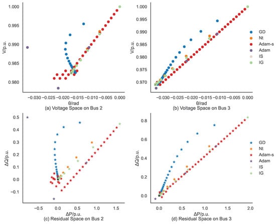
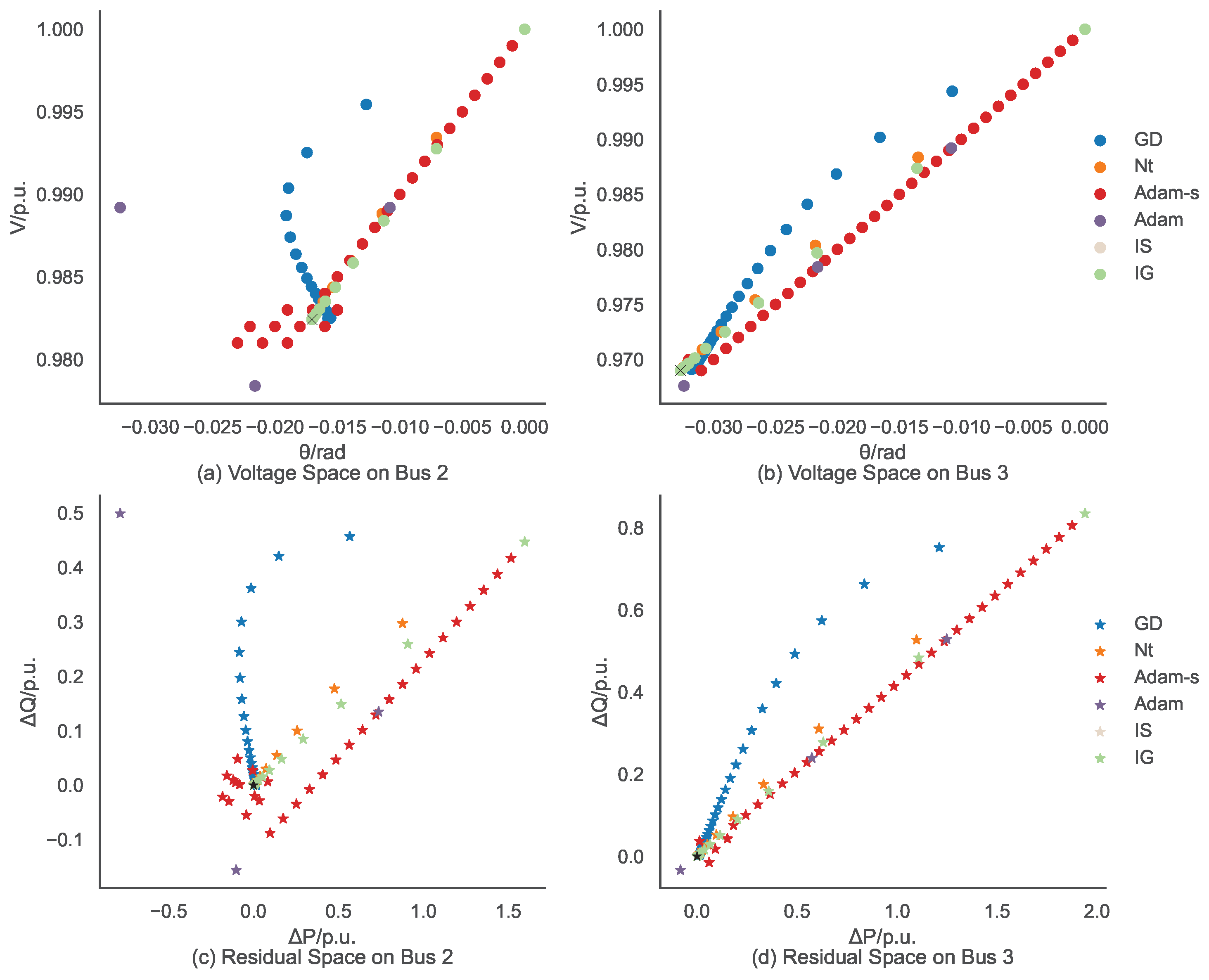
Using the solution obtained by Algorithm A1 as a ground truth benchmark, this section investigates how rapidly different optimization algorithms converge to the optimal solution. To understand the following example, it is important to remember that mappings are being dealt with between the two spaces: voltage $\mathbf{x}$ space and residual $\mathbf{y}$ space. Meanwhile, Bus 1 is a slack node and Bus 4 is a PV bus in case4gs. Therefore, only Bus 2 and 3 will be analyzed here. The ground truth at the left lower corner is shown with a thin black fork in voltage $\mathbf{x}$ space and a black five-pointed star in residual $\mathbf{y}$ space.

(1)

Voltage Space

Figure 1a,b reveal that the iterative trajectory of GD is characterized as a curvilinear path, initially exhibiting predominant lateral displacement along the $\theta$-axis followed by a progressive orientation toward the ground-truth solution. For other methods, they all formed a trajectory of the diagonal. However, Adam-s and Adam exhibit oscillations near the ground-truth solution. Furthermore, distinct variations in movement distances exhibited by the GD and Adam optimization algorithms are observed across different nodal points when subjected to comparative analysis between Bus 2 and Bus 3. This phenomenon arises due to the absence of gradient inversion or its incompleteness, which results in gradient scaling discrepancies. The GD is the absence of gradient inversion. Adam does not perform a full inversion via $\mathrm{diag}\left(J^{T}J\right)$ but uses the component-wise square root. The resultant approximation $\sqrt{\mathrm{diag}\left(J^{T}J\right)}\approx \sqrt{\mathrm{diag}\left(J^2\right)}\approx \mathrm{diag}\left(J\right)$ leads to parameter updates governed by $\Delta \approx \mathrm{sign}(-J)$, implementing dimension-wise fixed-step-size adjustments across all coordinates.

Figure 1. Voltage and residual space.

(2)

Residual Space

For GD, in the beginning, the dominance of the $\theta$ parameter is observed in voltage space, while the $\Delta P$ component predominantly governs the residual space. This aligns with established theoretical frameworks of power systems: there is the primary coupling relationship between active power and voltage phase angles—convergence dynamics of residual space similar to voltage space. While Adam demonstrates superior convergence characteristics in voltage space (Figure 1a), its residual space behavior in Figure 1c exhibits a trajectory that deviates from the diagonal accompanied by the $\Delta Q$ component’s predominance.

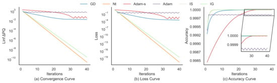
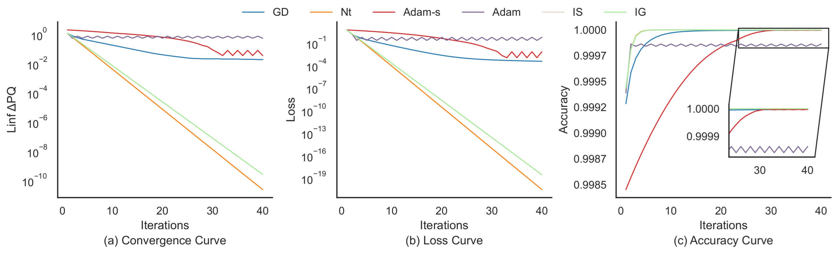
As evidenced by the comparative analysis in Figure 2a (Linf $\Delta$PQ denotes the inf-norm of $\Delta PQ$) and Figure 2b (Loss denotes the scalar residual loss $\mathcal{R}\left(\mathbf{x}\right)$), Nt demonstrates reliable Hessian matrix evaluation through strategic utilization of second-order information via $H^{-1}$ operator implementation. The optimization trajectory is characterized by predominant diagonal progression, corresponding to the theoretically optimal geodesic path, achieving significantly accelerated convergence dynamics compared to conventional implementations. Among comparative methods, IS and IG exhibit secondary optimization trajectories with enhanced proximity to ground-truth solutions. Central to this mechanism is the inverse operator implementation, which establishes gradient scaling compensation, thereby enhancing scale-invariant optimization properties. Notably, GD and Adam demonstrate a convergence loss curve $\mathcal{O}\left({10}^{-2}\right)$ significantly exceeding those of Nt, IS, and IG implementations.

Figure 2. Curve of convergence, loss and accuracy.

As shown in Figure 2, Nt achieves superior convergence precision, outperforming both IS and IG approaches, while GD and Adam come third.

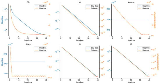
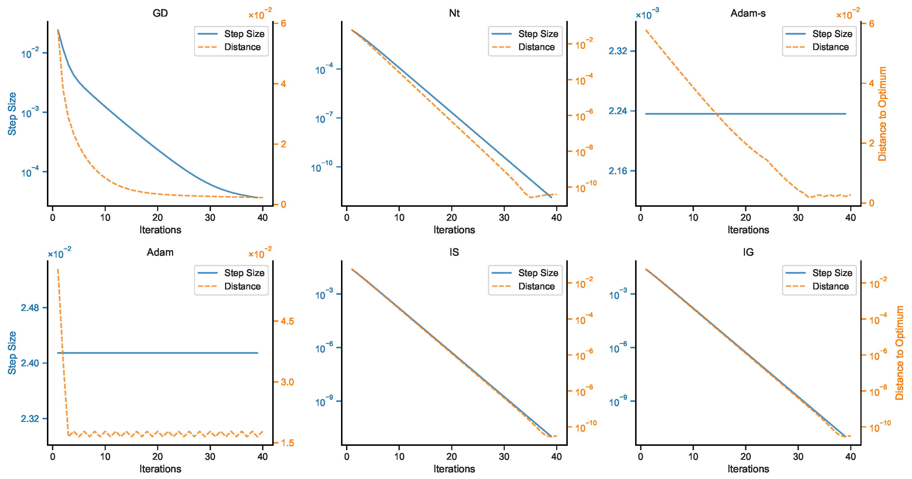
The convergence behaviors of six optimization algorithms—GD, Nt, Adam with reduced learning rate (Adam-s), Adam, IS, and IG—are evaluated over 40 iterations based on their step distances (Figure 3). All algorithms exhibit identical initial distances (0.0577), indicating uniform parameter initialization. However, their trajectories diverge significantly after the first iteration. GD follows a steady monotonic decay, reducing its distance by 96% by the 40th iteration (0.0577 → 0.0023), reflecting classic gradient-based convergence. In contrast, Nt demonstrates rapid early-stage stabilization, with its distance plummeting to $4.56\times {10}^{-11}$ by Iteration 40, suggesting superior local curvature exploitation. Adam-s achieves smoother convergence compared to standard Adam. For instance, in the first 33 iterations, Adam-s maintains a steady monotonic decay, while Adam oscillates between 0.0178 (even iterations) and 0.0165 (odd iterations) starting from the third iteration. This oscillation in Adam arises from its adaptive momentum mechanism. Adam-s mitigates this by tempering the learning rate and reducing update volatility by 53% in later stages (Iterations 30–40). The modified algorithm thus resembles “a gently meandering river,” avoiding abrupt fluctuations seen in Adam’s “turbulent cascades.” It can be seen from Figure 3 that the trajectories of IS and IG coincide. They exhibit intermediate convergence rates. Both algorithms stabilize earlier than GD and Adam but lag Nt.

Figure 3. Distance from the ground-truth solution of voltage.

Interestingly, when $\eta =1$, IG is equivalent to Algorithm A1.

Subsequently, the focus is directed toward the phase angle and magnitude of voltage, MW and MVar power, and branch MW and MVar flow. The corresponding errors are quantified by implementing Mean Absolute Error (MAE) and Root Mean Square Error (RMSE) metrics, respectively.

The error analysis in Table 3 shows that the IS and IG methodologies maintain comparable error magnitudes with the Nt approach while demonstrating marginal superiority in precision. Notably, the Adam algorithm exhibits error magnitudes two orders of magnitude higher than its Adam-s counterpart when configured with excessive step sizes. Regarding GD implementation, the voltage magnitude and active power errors demonstrate one to two orders of magnitude reduction compared to phase angle and reactive power discrepancies, respectively.

Table 3. Error Analysis of Testing Set.

Method		GD	Nt	Adam-s	Adam	IS	IG
MAE	$\theta /\mathrm{rad}$	9.52 × 10−4	9.11 × 10−12	7.82 × 10−4	5.16 × 10−3	8.36 × 10−12	8.36 × 10−12
	$V/\mathrm{p}.\mathrm{u}.$	3.89 × 10−5	8.25 × 10−12	3.54 × 10−4	3.35 × 10−3	7.11 × 10−12	7.11 × 10−12
	$P/\mathrm{MW}$ 1	1.18 × 10−2	2.43 × 10−10	9.76 × 10−3	2.34 × 10−1	2.23 × 10−10	2.23 × 10−10
	$Q/\mathrm{MVar}$	4.63 × 10−4	2.79 × 10−10	1.43 × 10−2	9.88 × 10−2	2.43 × 10−10	2.43 × 10−10
	$P_{ij}/\mathrm{MW}$ 2	1.67 × 10−2	2.66 × 10−10	1.49 × 10−2	1.71 × 10−1	2.32 × 10−10	2.32 × 10−10
	$Q_{ij}/\mathrm{MVar}$	3.10 × 10−3	3.03 × 10−10	1.49 × 10−2	1.08 × 10−1	2.76 × 10−10	2.76 × 10−10
MRSE	$\theta /\mathrm{rad}$	1.13 × 10−3	1.17 × 10−11	9.41 × 10−4	6.49 × 10−3	1.06 × 10−11	1.39 × 10−11
	$V/\mathrm{p}.\mathrm{u}.$	5.66 × 10−5	1.58 × 10−11	5.40 × 10−4	5.11 × 10−3	1.39 × 10−11	1.39 × 10−11
	$P/\mathrm{MW}$	1.39 × 10−2	4.18 × 10−10	1.24 × 10−2	3.19 × 10−1	3.20 × 10−10	3.20 × 10−10
	$Q/\mathrm{MVar}$	7.26 × 10−4	5.28 × 10−10	2.11 × 10−2	1.43 × 10−1	4.80 × 10−10	4.80 × 10−10
	$P_{ij}/\mathrm{MW}$	1.81 × 10−2	3.45 × 10−10	1.57 × 10−2	2.12 × 10−1	2.93 × 10−10	2.93 × 10−10
	$Q_{ij}/\mathrm{MVar}$	3.30 × 10−3	4.22 × 10−10	1.59 × 10−2	1.20 × 10−1	3.80 × 10−10	3.80 × 10−10

¹ P and Q are evaluated by (6). ² $P_{ij}$ and $Q_{ij}$ are evaluated using the following formulas: $P_{ij}=V_i^2{G}_{ij}-V_i{V}_j(G_{ij}cos{\delta }_{ij}+B_{ij}sin{\delta }_{ij})$; $Q_{ij}=V_i^2{B}_{ij}+V_i{V}_j(G_{ij}sin{\delta }_{ij}-B_{ij}cos{\delta }_{ij})$.

In conclusion, the GD is plagued by a gradient scaling discrepancy between voltage magnitudes and phase angles, exhibiting an order-of-magnitude difference between these parameters. For Adam, although the voltage magnitude and phase angle errors maintain comparable orders of magnitude, node-dependent scaling variations are observed across different network nodes (attributed to incomplete gradient scaling compensation resulting from partial gradient matrix correction through diagonal inverse matrix utilization). This scaling inconsistency is similar in GD implementations due to the absence of gradient scaling compensation. In contrast, the Nt, IS, and IG methodologies effectively resolve the gradient scaling challenge through comprehensive inverse matrix implementation, achieving complete gradient compensation across all parameters.

3.2. Physics-Based Deep Learning

The Nt is excluded from the current analytical framework due to the inherent Hessian matrix construction and inversion requirement, which entails significant computational overhead. The IS methodology is analogously constrained by equivalent computational requirements involving Hessian matrix construction and inversion processes. Furthermore, as established in Section 3.1, its performance is demonstrated to exhibit equivalence with IG. Consequently, Nt and IS are deliberately omitted from the systematic investigation presented in this section. Three methodological approaches, comprising GD, Adam, and HIG, are employed to demonstrate DP learning systematically. In particular, the batch size parameter was assigned 16. Other settings are the same as in Table 1. The case settings are as follows (Table 4):

Table 4. Case Setting.

Method	Optimizer 1	$\lambda$ 2	Epoch
DP-GD	$\Delta {\Theta }_{\mathrm{GD}}=-\lambda {\displaystyle \frac{\partial \mathcal{R}}{\partial \Theta }}$	0.0001	50
DP-Adam	$\Delta {\Theta }_{\mathrm{Adam}}=-\lambda {\sqrt{\mathrm{diag}\left[{\left({\displaystyle \frac{\partial \mathbf{x}}{\partial \Theta }}\right)}^T{\displaystyle \frac{\partial \mathbf{x}}{\partial \Theta }}\right]}}^{-1}\left({\displaystyle \frac{\partial \mathbf{x}}{\partial \Theta }}{\displaystyle \frac{\partial \mathbf{y}}{\partial \mathbf{x}}}{\displaystyle \frac{\partial \mathcal{R}}{\partial \mathbf{y}}}\right)$	0.0001
DP-HIG	$\Delta {\Theta }_{\mathrm{HIG}}=-\lambda {\left({\displaystyle \frac{\partial \mathbf{x}}{\partial \Theta }}\right)}^{-1/2}\left({\displaystyle \frac{\partial \mathbf{y}}{\partial \mathbf{x}}}{\displaystyle \frac{\partial \mathcal{R}}{\partial \mathbf{y}}}\right)$	0.01

¹$\Theta$ denotes the parameter of weights and bias for NN. ² $\lambda$ denotes learning rate.

The parameterization of learning rates is systematically investigated through an order-of-magnitude-based methodology. Divergent behavior manifests when the learning rate exceeds the value of Table 4 by one order of magnitude, while suboptimal convergence characteristics are identified when reduced by an equivalent logarithmic scale.

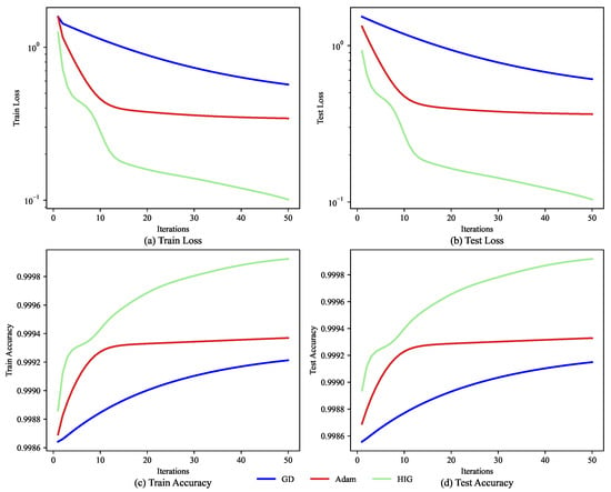
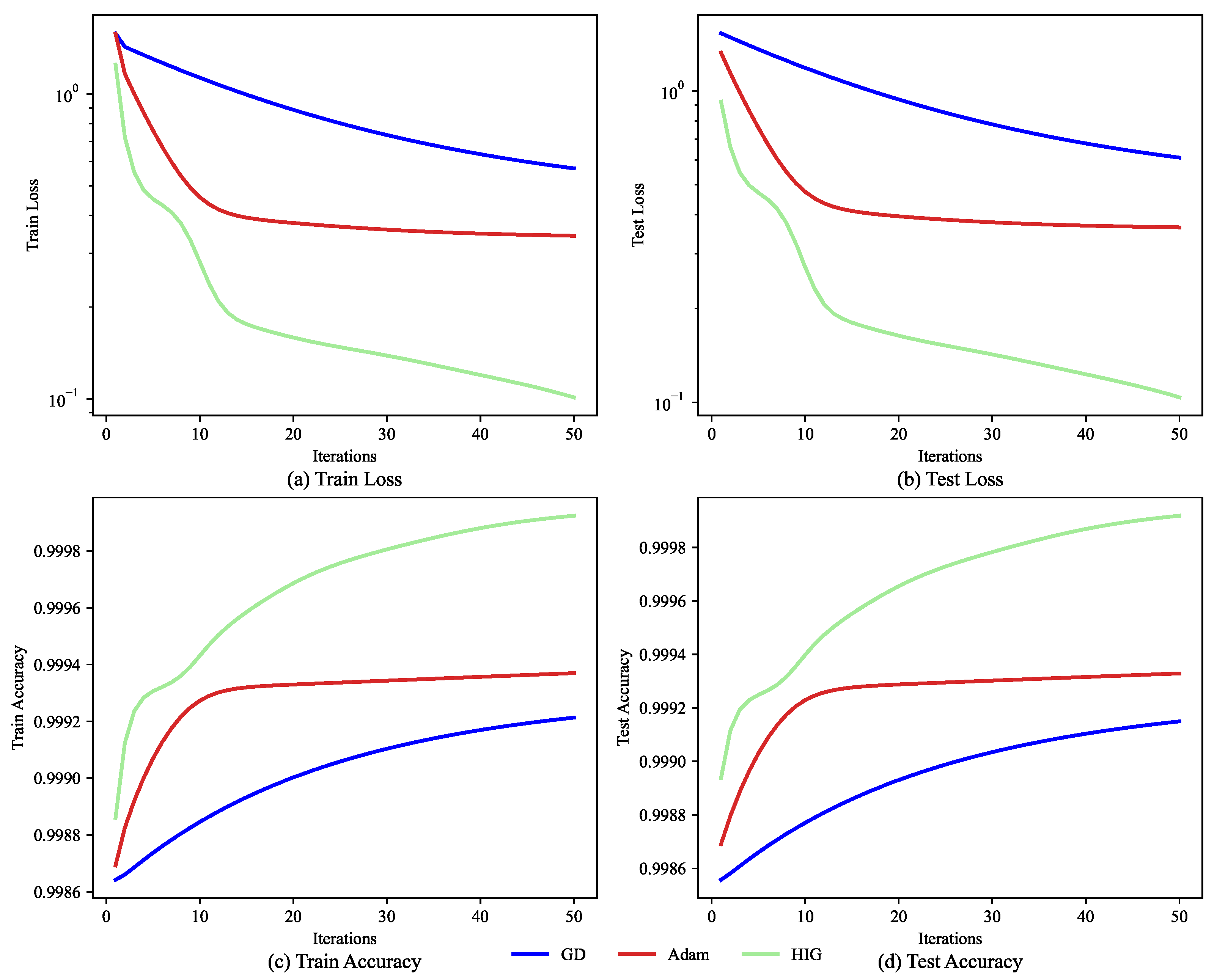
As illustrated in Figure 4, the superior convergence performance of Adam over GD is observed owing to the diagonal inverse compensation term diag${\sqrt{\mathrm{diag}\left[{\left({\displaystyle \frac{\partial \mathbf{x}}{\partial \Theta }}\right)}^T{\displaystyle \frac{\partial \mathbf{x}}{\partial \Theta }}\right]}}^{-1}$. Adam achieves convergence after merely 10 iterations, whereas GD demonstrates a gradual decline even at the 50th iteration with notably inferior loss values and accuracy compared to Adam. Regarding HIG, it is remarkably noted that preserving both diagonal inverse information and substantial non-diagonal information enables the realization of a distinctive two-phase accelerated convergence pattern.

Figure 4. Loss and Accuracy Curves.

During the initial phase (first acceleration), HIG attains equivalent convergence performance to Adam within only five iterations—50% faster than Adam’s 10 iterations. This enhanced convergence rate is attributed to the dominant influence of diagonal inverse information, which combines with substantial non-diagonal information utilization. Following two transitional iterations serving as buffer periods, the secondary acceleration phase is activated where non-diagonal information becomes predominant in governing convergence. This secondary acceleration persists until the 14th iteration, after which the loss value continues descending at a consistent rate (through the 50th iteration) due to the comprehensive utilization of both diagonal and substantial non-diagonal inverse information. Notably, while maintaining progressive loss reduction, accuracy stabilizes gradually during later iterations.

As demonstrated in Table 5, the HIG method exhibits superior generalization capability compared to conventional GD and Adam optimization approaches. Significant discrepancies in loss values between training and test sets are quantified as 0.041 and 0.022 for GD and Adam, respectively, both maintaining an order of magnitude of 1. In contrast, the HIG framework exhibits a remarkably reduced discrepancy of 0.003 (2 orders of magnitude), representing an order-of-magnitude improvement in generalization performance.

Table 5. Analysis of Training and Testing Sets.

Method		GD	Adam	HIG
Train	$\mathcal{R}$	5.70 × 10−1	3.43 × 10−1	1.01 × 10−1
	${\mathrm{R}2}_{\mathrm{Acc}}$ /%	99.92	99.94	99.99
Test	$\mathcal{R}$	6.11 × 10−1	3.65 × 10−1	1.04 × 10−1
	${\mathrm{R}2}_{\mathrm{Acc}}$ /%	99.91	99.93	99.99

Furthermore, critical limitations are identified in the precision characteristics of conventional methods. Suboptimal accuracy levels below 99.95% are recorded for GD and Adam, accompanied by measurable dataset-dependent variations. The proposed HIG framework achieves a state-of-the-art accuracy of 99.99% while demonstrating complete consistency between training and test environments. This performance enhancement is particularly noteworthy as it simultaneously addresses precision optimization and cross-dataset stability—two critical challenges in contemporary optimization algorithm design.

As presented in Table 6, distinct precision characteristics are observed between GD and Adam optimizers in voltage phase angle (${10}^{-2}$) and magnitude (${10}^{-3}$) estimation, with superior performance being demonstrated in magnitude calculations. In contrast, the HIG method exhibits identical precision levels (${10}^{-3}$) for phase angle and magnitude estimation. Notably, the one-order-of-magnitude-inferior voltage estimation accuracy observed in GD and Adam implementations results in comparable precision levels (${10}^{-1}$) regarding MW and MVar calculations. Furthermore, due to the equivalent voltage estimation precision (${10}^{-3}$) achieved by HIG, its MW evaluation demonstrates enhanced accuracy (${10}^{-2}$) compared with MVar estimation (${10}^{-1}$), reflecting improved physical consistency in power system solutions.

Table 6. Error Analysis of Testing Set.

Method		GD	Adam	HIG
MAE	$\theta /\mathrm{rad}$	1.34 × 10−2	1.25 × 10−2	2.21 × 10−3
	$V/\mathrm{p}.\mathrm{u}.$	5.40 × 10−3	3.59 × 10−3	3.35 × 10−3
	$P/\mathrm{MW}$	3.06 × 10−1	2.56 × 10−1	4.52 × 10−2
	$Q/\mathrm{MVar}$	2.02 × 10−1	1.45 × 10−1	1.33 × 10−1
	$P_{ij}/\mathrm{MW}$	2.92 × 10−1	2.70 × 10−1	4.94 × 10−2
	$Q_{ij}/\mathrm{MVar}$	2.17 × 10−1	1.54 × 10−1	1.39 × 10−1
MRSE	$\theta /\mathrm{rad}$	1.64 × 10−2	1.55× 10−2	2.66 × 10−3
	$V/\mathrm{p}.\mathrm{u}.$	8.47 × 10−3	5.47 × 10−3	5.11 × 10−3
	$P/\mathrm{MW}$	4.08 × 10−1	3.31 × 10−1	5.90 × 10−2
	$Q/\mathrm{MVar}$	3.14 × 10−1	2.21 × 10−1	2.03 × 10−1
	$P_{ij}/\mathrm{MW}$	3.49 × 10−1	3.08 × 10−1	5.92 × 10−2
	$Q_{ij}/\mathrm{MVar}$	2.48 × 10−1	1.74 × 10−1	1.53 × 10−1

Suppose the parameterized voltage method is not employed and only fully connected layers are used as the output layer. In that case, the output values obtained through residual term optimization using GD, Adam, and HIG methods will demonstrate significant degradation. The voltage magnitude outputs will substantially deviate from expected values, reaching a maximum magnitude of merely ${10}^{-2}$ order magnitude, considerably lower than the voltage magnitude constraint range of 0.94–1.06 p.u. Due to the unsatisfactory performance of their convergence and accuracy curves, these results are omitted from the presentation in this paper. Interested readers are encouraged to reproduce the experiments independently for further validation.

3.3. Scalability Analysis and PINN

As shown in Table 7, the simulation configuration for this section was systematically designed by (2). The remaining settings are the same as Table 1. Concurrently, the supervised learning (SL) methodology (SL only adopts the GD optimizer), where ${\alpha }_0=1$ and ${\alpha }_1=0$, was strategically incorporated as a comparative baseline framework to enable systematic performance evaluation. The ${\alpha }_0$ and ${\alpha }_1$ are set to 0.5 to harmonize the contributions between conventional loss components and residual terms in PINN. This equilibrium configuration was deliberately implemented to ensure equivalent gradient propagation magnitudes during backpropagation iterations.

Table 7. Simulation Configuration.

Test System	${\alpha }_{\mathbf{0}}$	${\alpha }_{\mathbf{1}}$	Method	$\lambda$	Epoch
case4gs	1.0	0.0	SL	0.01	50
	0.0	1.0	DP-GD	0.0001
			DP-Adam	0.0001
			DP-HIG	0.01
	0.5	0.5	PINN-GD	0.0001
			PINN-Adam	0.001
			PINN-HIG	0.01
case30	1.0	0.0	SL	0.01
	0.0	1.0	DP-GD	0.00001
			DP-Adam	0.0001
			DP-HIG	0.001
	0.5	0.5	PINN-GD	0.0001
			PINN-Adam	0.001
			PINN-HIG	0.01
case118	1.0	0.0	SL	0.01
	0.0	1.0	DP-GD	0.000001
			DP-Adam	0.00001
			DP-HIG	0.0001
	0.5	0.5	PINN-GD	0.000001
			PINN-Adam	0.00001
			PINN-HIG	0.0001

Table 8 reveals distinct performance patterns across varying system scales. For case4gs and case30 of power systems, comparable accuracy attainment rates exceeding 99% are observed among all investigated methodologies. However, significant performance degradation is identified in case118 system simulations. The SL maintains a 96% accuracy threshold, whereas substantial precision deterioration below 40% is recorded for differentiable physics variants (DP-GD, DP-Adam, DP-HIG). Similar performance limitations are demonstrated in physics-informed neural network implementations (PINN-GD, PINN-Adam), exhibiting error characteristics analogous to their DP. Notably, the PINN-HIG framework achieves a remarkable 27% accuracy enhancement compared with the DP-HIG methodology, demonstrating the effectiveness of PINN-HIG in neural network-based power flow computation.

Table 8. Accuracy of Training and Testing Sets.

Test System	Method	Train ${\mathbf{R}2}_{\mathbf{Acc}}$ /%	Test ${\mathbf{R}2}_{\mathbf{Acc}}$ /%
case4gs	SL	99.87	99.86
	DP-GD	99.91	99.90
	DP-Adam	99.93	99.93
	DP-HIG	99.97	99.97
	PINN-GD	99.89	99.88
	PINN-Adam	99.95	99.94
	PINN-HIG	99.94	99.94
case30	SL	99.83	99.84
	DP-GD	99.48	99.46
	DP-Adam	99.48	99.47
	DP-HIG	99.48	99.46
	PINN-GD	99.59	99.58
	PINN-Adam	99.81	99.82
	PINN-HIG	99.83	99.84
case118	SL	96.29	96.37
	DP-GD	35.75	35.87
	DP-Adam	36.25	36.39
	DP-HIG	37.29	37.49
	PINN-GD	35.63	35.75
	PINN-Adam	37.76	37.91
	PINN-HIG	64.29	64.70

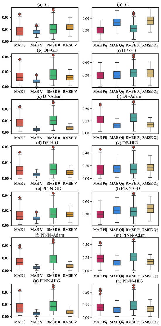
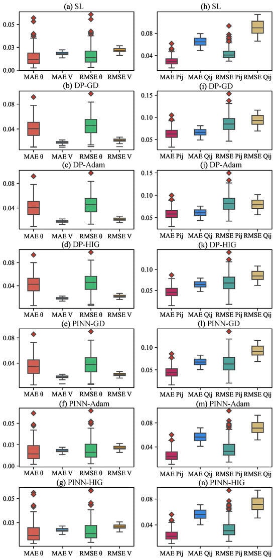
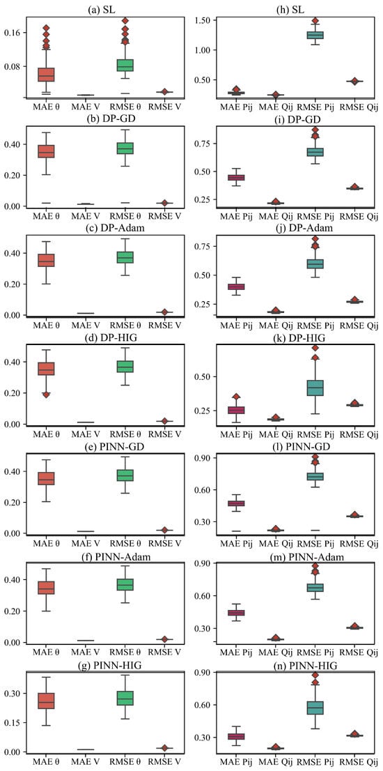
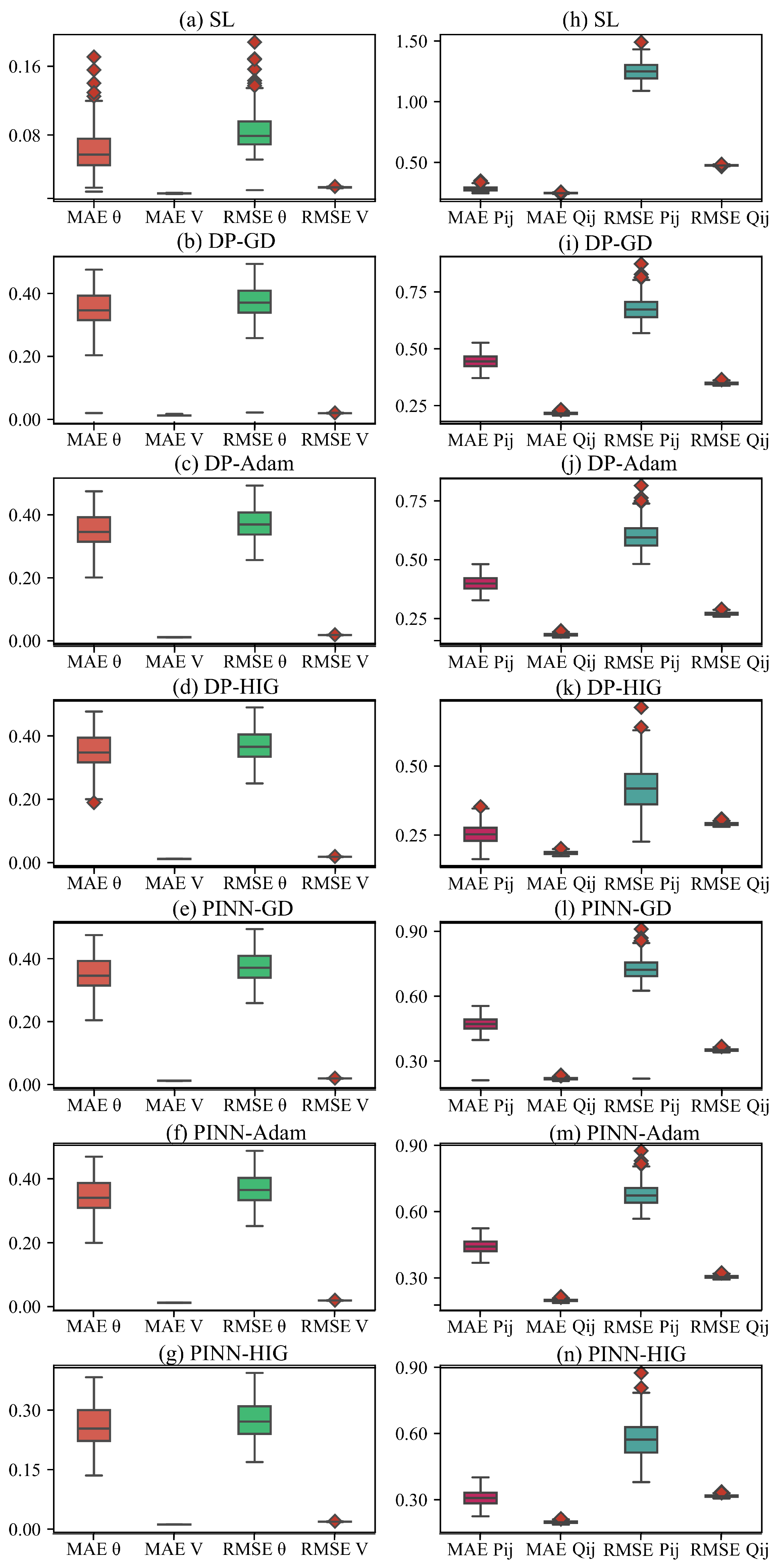
The comparative analysis of computational accuracy presented in Figure 5, Figure 6 and Figure 7 ((a–g) and (h–n) denote SL, DP-GD, DP-Adam, DP-HIG, PINN-GD, PINN-Adam and PINN-HIG, respectively) reveals a notable divergence in performance characteristics. While superior voltage estimation accuracy is consistently maintained through SL paradigms, a statistically significant precision degradation in branch power flow calculation is systematically observed compared with other methodologies. This discrepancy between voltage preservation capability and branch power flow computation fidelity highlights critical limitations in deep learning architectures for physics power system modeling tasks.

Figure 5. Error comparison of voltage and branch power flow of case4.

Figure 6. Error comparison of voltage and branch power flow of case30.

Figure 7. Error comparison of voltage and branch power flow of case118.

The marked performance deterioration observed in the case118 system for DP, PINN-GD, and PINN-Adam is primarily attributed to architectural constraints inherent in fully connected neural network configurations, particularly regarding layer depth and neuron density limitations imposed by computational resource boundaries. This critical restriction on DL fundamentally compromises the model expressivity required for capturing high-dimensional nonlinear interactions characteristic of large-scale power grid dynamics, ultimately constraining the algorithms’ capability to maintain solution fidelity in complex grid operation scenarios. The enhanced computational capability demonstrated by the PINN-HIG is fundamentally enabled through innovative gradient optimization mechanisms. By systematically exploring latent solution space characteristics within neural network architectures, superior parameter utilization efficiency is achieved, effectively maintaining algorithmic stability.

4. Conclusions

This study addresses the limitations of conventional PF solvers and black-box DL approaches by proposing a PINN framework integrated with a novel HIG mechanism. By systematically analyzing the gradient scaling phenomenon in PF-oriented neural optimization, this work explains a key reason why existing neural networks are often difficult to stably integrate with physical models, namely the scaling inconsistency caused by insufficient inverse compensation during gradient propagation. Based on this mechanism-level insight, a gradient matrix compensation strategy is developed to improve training stability and to bridge the gap between data-driven learning and physical constraints in power-system optimization.

The main findings of this work can be summarized as follows:

• Gradient scaling and optimization stability: The inherent instability of gradient-based optimization in PF problems is traced to insufficient inverse matrix compensation. The proposed residual-driven HIG framework mitigates gradient scaling distortion through truncated SVD-based compensation, thereby achieving more stable training dynamics. On benchmark systems such as case4gs and case30, the HIG-based method demonstrates faster and more stable convergence, reaching 99% accuracy and achieving approximately 50% acceleration compared with Adam-based optimization.
• Hard physical constraint enforcement: By parameterizing voltage variables and introducing differentiable activation functions, hard operational constraints can be enforced while preserving end-to-end differentiability. This design eliminates the need for additional post-processing and reduces voltage magnitude errors to the order of ${10}^{-3}$.
• Scalability and generalization: The proposed framework exhibits promising scalability and generalization performance on standard PF benchmarks. In particular, it achieves 65% accuracy on case118, significantly outperforming baseline physics-informed methods (below 38%). By combining HIG compensation with physically constrained learning, the method provides more consistent voltage estimation and improved robustness across datasets. From a theoretical perspective, the universal approximation capability of neural networks also supports the representational adequacy of the proposed model for PF dynamics.

Despite these encouraging results, the present study still has several limitations. Due to the structural constraints imposed by the fully connected neural architecture and the associated computational burden, the largest benchmark investigated in this work is limited to the 118-bus test system. In practice, the current implementation remains memory-intensive, which restricts a more comprehensive study on larger-scale systems with stronger network coupling and more pronounced uncertainty. Therefore, the present paper should be understood primarily as a mechanism-oriented study that reveals the gradient scaling bottleneck in physics-integrated neural optimization, rather than as a complete large-scale deployment framework.

Future work will proceed in several directions. First, inspired by recent progress in data-and-model-driven acceleration for large-scale network-constrained optimization under uncertainty [17], the proposed framework will be extended toward larger and more complex power systems, especially those with high renewable energy penetration, for applications such as optimal power flow (OPF), security-constrained unit commitment (SCUC), and real-time grid management. In particular, reducing memory consumption and improving the tractability of Jacobian- or Hessian-related compensation under large-scale constraints will be essential for practical deployment.

Second, motivated by recent advances in uncertainty-aware neural computation, such as quantum interval neural networks for uncertain static analysis [20], future research will explore uncertainty-aware extensions of the HIG-based PINN so that interval uncertainty, parameter variability, and operating-condition ambiguity can be incorporated more explicitly into the learning and optimization process. Along a similar line, the robustness of the convergence process may benefit from ideas developed in dual-network recursive interval type-2 fuzzy neural networks for fault diagnosis [21], particularly in scenarios involving noisy measurements, uncertain system states, and recursive error propagation.

Third, reliability-oriented validation will be further strengthened. Recent developments in self-supervised insulation-condition evaluation using hypergraph neural networks [18] and in incipient fault detection for inverter systems [19] suggest that future physics-informed learning frameworks should not only satisfy physical equations and operational constraints, but also maintain robustness under degraded sensing conditions, perturbations, and fault scenarios. In this sense, the proposed HIG-based framework provides a mechanism-oriented foundation, while uncertainty quantification, fault tolerance, and reliability-aware learning constitute important future extensions.

Overall, by eliminating the need for explicit data normalization and enabling seamless integration with physics-informed optimization algorithms for joint co-optimization, the HIG-based learning framework offers a promising path toward interpretable neural computation for nonlinear power-system problems. Through this design, the physical interpretability of power-system variables can be preserved while the flexibility of deep learning is effectively leveraged. We believe that this balance between physical consistency and learning capability will remain essential for future co-optimization frameworks in increasingly complex and uncertainty-rich power grids.

Appendix A.1. General Nonlinear Model and Unified Iterative Formulation

Consider the nonlinear algebraic system

$$f\left(x\right)=0,$$

(A1)

where $x\in {\mathbb{R}}^m$ is the unknown state vector and $f:{\mathbb{R}}^m\to {\mathbb{R}}^m$ is a nonlinear mapping. Let $x^{*}$ denote an exact solution of (A1), i.e.,

$$f\left(x^{*}\right)=0.$$

(A2)

Let the Jacobian matrix of $f\left(x\right)$ be denoted by

$$J\left(x\right)={\displaystyle \frac{\partial f\left(x\right)}{\partial x}}.$$

(A3)

A unified representation of the three iterative methods can be written as

$$x^{(k+1)}=x^{\left(k\right)}-M\left(x^{\left(k\right)}\right)f\left(x^{\left(k\right)}\right),$$

(A4)

where $M\left(x\right)$ is a method-dependent matrix-valued operator. Specifically, the three methods considered in this appendix are defined as follows:

• Newton’s method:

  $$M\left(x\right)=J{\left(x\right)}^{-1};$$

  (A5)
• Half-inverse gradient method:

  $$M\left(x\right)=J{\left(x\right)}^{-1/2};$$

  (A6)
• Gradient-descent-type method:

  $$M\left(x\right)=I,$$

  (A7)

where I denotes the identity matrix. Here, $J{\left(x\right)}^{-1/2}$ denotes a matrix inverse square root, which is well-defined when $J\left(x\right)$ admits a suitable square root, for example, when $J\left(x\right)$ is symmetric positive definite in a neighborhood of the solution.

Appendix A.2. Assumptions

The following assumptions are adopted throughout the local convergence analysis:

Assumption A1.

There exists a solution $x^{*}\in {\mathbb{R}}^m$ such that $f\left(x^{*}\right)=0$.

Assumption A2.

The mapping $f\left(x\right)$ is twice continuously differentiable in an open neighborhood $\mathcal{N}\left(x^{*}\right)$, namely,

$$f\in C^2\left(\mathcal{N}\left(x^{*}\right)\right).$$

(A8)

Assumption A3.

The Jacobian at the solution is nonsingular, i.e.,

$$detJ\left(x^{*}\right)\ne 0.$$

(A9)

Assumption A4.

For the half-inverse gradient method, $J\left(x\right)$ admits a well-defined inverse square root $J{\left(x\right)}^{-1/2}$ in a neighborhood of $x^{*}$. A sufficient condition is that $J\left(x\right)$ be symmetric positive definite in that neighborhood.

Assumption A5.

The initial point $x^{\left(0\right)}$ is sufficiently close to $x^{*}$, such that all local Taylor expansions and asymptotic estimates used below are valid.

Assumptions A1–A5 are standard in local convergence theory. Under these conditions, the asymptotic behavior of the three iterative methods can be analyzed in a unified manner.

Appendix A.3. Error Definition and Common Local Expansion

Define the iteration error by

$$e^{\left(k\right)}=x^{\left(k\right)}-x^{*}.$$

(A10)

Since $f\left(x^{*}\right)=0$ and $f\in C^2$, a second-order Taylor expansion around $x^{*}$ yields

$$f\left(x^{\left(k\right)}\right)=f(x^{*}+e^{\left(k\right)})=J^{*}{e}^{\left(k\right)}+O\left(\parallel e^{\left(k\right)}{\parallel }^2\right),$$

(A11)

where

$$J^{*}:=J\left(x^{*}\right).$$

(A12)

If $M\left(x\right)$ is continuous in a neighborhood of $x^{*}$, then

$$M\left(x^{\left(k\right)}\right)=M\left(x^{*}\right)+O\left(\parallel e^{\left(k\right)}\parallel \right).$$

(A13)

Substituting (A11) and (A13) into the unified iteration formula (A4) gives

$$\begin{array}{cc}\hfill e^{(k+1)}& =x^{(k+1)}-x^{*}\hfill \\ \hfill & =x^{\left(k\right)}-x^{*}-M\left(x^{\left(k\right)}\right)f\left(x^{\left(k\right)}\right)\hfill \\ \hfill & =e^{\left(k\right)}-\left(M\left(x^{*}\right)+O(\parallel e^{\left(k\right)}\parallel )\right)\left(J^{*}{e}^{\left(k\right)}+O(\parallel e^{\left(k\right)}{\parallel }^2)\right)\hfill \\ \hfill & =\left(I-M\left(x^{*}\right)J^{*}\right)e^{\left(k\right)}+O\left(\parallel e^{\left(k\right)}{\parallel }^2\right).\hfill \end{array}$$

(A14)

Equation (A14) is the common leading-order error recursion for all three methods.

Appendix A.4. Newton’s Method

For Newton’s method, $M\left(x\right)=J{\left(x\right)}^{-1}$, and the iterative formula becomes

$$x^{(k+1)}=x^{\left(k\right)}-J{\left(x^{\left(k\right)}\right)}^{-1}f\left(x^{\left(k\right)}\right).$$

(A15)

At the solution point,

$$M\left(x^{*}\right)J^{*}=J^{*-1}{J}^{*}=I.$$

(A16)

Therefore, from (A14),

$$e^{(k+1)}=O\left(\parallel e^{\left(k\right)}{\parallel }^2\right).$$

(A17)

Equivalently, there exists a constant $C_{\mathrm{N}}>0$ such that

$$\parallel e^{(k+1)}\parallel \le C_{\mathrm{N}}{\parallel e^{\left(k\right)}\parallel }^2\mathrm{for}\mathrm{sufficiently}\mathrm{large}k.$$

(A18)

Hence, Newton’s method exhibits local quadratic convergence. This result follows from the complete cancellation of the first-order error term in (A14).

Appendix A.5. Half-Inverse Gradient Method

For the half-inverse gradient method, $M\left(x\right)=J{\left(x\right)}^{-1/2}$, and the iteration is written as

$$x^{(k+1)}=x^{\left(k\right)}-J{\left(x^{\left(k\right)}\right)}^{-1/2}f\left(x^{\left(k\right)}\right).$$

(A19)

Substituting $M\left(x^{*}\right)=J^{*-1/2}$ into (A14) yields

$$\begin{array}{cc}\hfill e^{(k+1)}& =\left(I-J^{*-1/2}{J}^{*}\right)e^{\left(k\right)}+O\left(\parallel e^{\left(k\right)}{\parallel }^2\right)\hfill \\ \hfill & =\left(I-J^{*1/2}\right)e^{\left(k\right)}+O\left(\parallel e^{\left(k\right)}{\parallel }^2\right).\hfill \end{array}$$

(A20)

Thus, if the spectral radius satisfies

$$\rho \left(I-J^{*1/2}\right)<1,$$

(A21)

then the method is locally linearly convergent. More precisely, there exist constants $q_{\mathrm{H}}\in (0,1)$ and $C_{\mathrm{H}}>0$ such that

$$\parallel e^{(k+1)}\parallel \le q_{\mathrm{H}}\parallel e^{\left(k\right)}\parallel +C_{\mathrm{H}}{\parallel e^{\left(k\right)}\parallel }^2.$$

(A22)

When k is sufficiently large and $\parallel e^{\left(k\right)}\parallel$ is small, the quadratic remainder becomes negligible and

$$\parallel e^{(k+1)}\parallel \approx q_{\mathrm{H}}\parallel e^{\left(k\right)}\parallel ,q_{\mathrm{H}}\approx \rho \left(I-J^{*1/2}\right).$$

(A23)

Therefore, the half-inverse gradient method generally exhibits local linear convergence rather than quadratic convergence.

• Special Case: Symmetric Positive Definite Jacobian

If $J^{*}$ is symmetric positive definite, then it can be diagonalized as

$$J^{*}=Q\Lambda Q^{\top },\Lambda =\mathrm{diag}({\lambda }_1,{\lambda }_2,\dots ,{\lambda }_m),{\lambda }_i>0.$$

(A24)

Hence,

$$J^{*1/2}=Q{\Lambda }^{1/2}{Q}^{\top },$$

(A25)

and the eigenvalues of $I-J^{*1/2}$ are

$$1-\sqrt{{\lambda }_i},i=1,2,\dots ,m.$$

(A26)

The local convergence condition (A21) is then equivalent to

$$|1-\sqrt{{\lambda }_i}|<1,i=1,2,\dots ,m,$$

(A27)

or, equivalently,

$$0<{\lambda }_i<4,i=1,2,\dots ,m.$$

(A28)

In this case, the asymptotic linear convergence factor can be written as

$$q_{\mathrm{H}}=\underset{i}{max}|1-\sqrt{{\lambda }_i}|.$$

(A29)

Appendix A.6. Gradient-Descent-Type Method

For the gradient-descent-type method, $M\left(x\right)=I$, and the iteration becomes

$$x^{(k+1)}=x^{\left(k\right)}-f\left(x^{\left(k\right)}\right).$$

(A30)

From (A14), the corresponding error recursion is

$$e^{(k+1)}=\left(I-J^{*}\right)e^{\left(k\right)}+O\left(\parallel e^{\left(k\right)}{\parallel }^2\right).$$

(A31)

Hence, if

$$\rho (I-J^{*})<1,$$

(A32)

then the method is locally linearly convergent. In particular, there exist constants $q_{\mathrm{G}}\in (0,1)$ and $C_{\mathrm{G}}>0$ such that

$$\parallel e^{(k+1)}\parallel \le q_{\mathrm{G}}\parallel e^{\left(k\right)}\parallel +C_{\mathrm{G}}{\parallel e^{\left(k\right)}\parallel }^2.$$

(A33)

Therefore, asymptotically,

$$\parallel e^{(k+1)}\parallel \approx q_{\mathrm{G}}\parallel e^{\left(k\right)}\parallel ,q_{\mathrm{G}}\approx \rho (I-J^{*}).$$

(A34)

Thus, the gradient-descent-type method also exhibits local linear convergence.

Under the symmetric positive definite assumption in (A24), the eigenvalues of $I-J^{*}$ are

$$1-{\lambda }_i,i=1,2,\dots ,m.$$

(A35)

Accordingly, the convergence condition (A32) becomes

$$|1-{\lambda }_i|<1,i=1,2,\dots ,m,$$

(A36)

which is equivalent to

$$0<{\lambda }_i<2,i=1,2,\dots ,m.$$

(A37)

The corresponding asymptotic linear convergence factor is

$$q_{\mathrm{G}}=\underset{i}{max}|1-{\lambda }_i|.$$

(A38)

Appendix A.7. Comparison of Convergence Rates

Based on the above derivations, the leading-order local error recursions of the three methods can be summarized as follows:

• Newton’s method:

  $$e^{(k+1)}=O\left(\parallel e^{\left(k\right)}{\parallel }^2\right);$$

  (A39)
• Half-inverse gradient method:

  $$e^{(k+1)}=\left(I-J^{*1/2}\right)e^{\left(k\right)}+O\left(\parallel e^{\left(k\right)}{\parallel }^2\right);$$

  (A40)
• Gradient-descent-type method:

  $$e^{(k+1)}=\left(I-J^{*}\right)e^{\left(k\right)}+O\left(\parallel e^{\left(k\right)}{\parallel }^2\right).$$

  (A41)

It can be seen that Newton’s method removes the entire first-order error term and therefore achieves quadratic convergence. By contrast, the half-inverse gradient method and the gradient-descent-type method retain a nonzero linear term and, consequently, are generally only linearly convergent in the local regime.

For the symmetric positive definite case, the asymptotic contraction factors are

$$q_{\mathrm{H}}=\underset{i}{max}|1-\sqrt{{\lambda }_i}|,q_{\mathrm{G}}=\underset{i}{max}|1-{\lambda }_i|.$$

(A42)

Since the square-root transformation compresses the eigenvalue distribution, the half-inverse gradient method usually has a smaller contraction factor than the gradient-descent-type method, i.e.,

$$q_{\mathrm{H}}<q_{\mathrm{G}}$$

(A43)

for a broad class of practically relevant spectra. Therefore, the local convergence-speed ranking is generally expressed as

$$\mathrm{Newton}’\mathrm{s}\mathrm{method}>\mathrm{Half}\text{-}\mathrm{inverse}\mathrm{gradient}\mathrm{method}>\mathrm{Gradient}\text{-}\mathrm{descent}\text{-}\mathrm{type}\mathrm{method},$$

(A44)

where the symbol “>” indicates a faster asymptotic local convergence rate.

It should be emphasized that the above comparison is local and asymptotic. In other words, it holds when the iterates are sufficiently close to the exact solution and the assumptions stated in Appendix A.2 are satisfied.

Appendix A.8. Summary of the Main Results

The main local convergence results derived above can be summarized as

$$\parallel e^{(k+1)}\parallel \le C_{\mathrm{N}}{\parallel e^{\left(k\right)}\parallel }^2$$

(A45)

for Newton’s method,

$$\parallel e^{(k+1)}\parallel \le q_{\mathrm{H}}\parallel e^{\left(k\right)}\parallel +C_{\mathrm{H}}{\parallel e^{\left(k\right)}\parallel }^2,q_{\mathrm{H}}=\rho \left(I-J^{*1/2}\right)<1$$

(A46)

for the half-inverse gradient method, and

$$\parallel e^{(k+1)}\parallel \le q_{\mathrm{G}}\parallel e^{\left(k\right)}\parallel + C_{\mathrm{G}}{\parallel e^{\left(k\right)}\parallel }^2,q_{\mathrm{G}}=\rho (I-J^{*})<1$$

(A47)

for the gradient-descent-type method.

Therefore, Newton’s method is quadratically convergent, whereas the half-inverse gradient method and the gradient-descent-type method are, in general, linearly convergent. Among the latter two methods, the half-inverse gradient method usually converges faster because its leading-order contraction factor is typically smaller.

Table A1. Comparison of the local convergence properties of the three methods.

Method	Iteration Formula	Leading Error Term
Newton’s method	$x^{(k+1)}=x^{\left(k\right)}-J{\left(x^{\left(k\right)}\right)}^{-1}f\left(x^{\left(k\right)}\right)$	$O(\parallel e^{\left(k\right)}{\parallel }^2)$
Half-inverse gradient method	$x^{(k+1)}=x^{\left(k\right)}-J{\left(x^{\left(k\right)}\right)}^{-1/2}f\left(x^{\left(k\right)}\right)$	$\left(I-J^{*1/2}\right)e^{\left(k\right)}+O(\parallel e^{\left(k\right)}{\parallel }^2)$
Gradient-descent-type method	$x^{(k+1)}=x^{\left(k\right)}-f\left(x^{\left(k\right)}\right)$	$\left(I-J^{*}\right)e^{\left(k\right)}+O(\parallel e^{\left(k\right)}{\parallel }^2)$

Table A1. Comparison of the local convergence properties of the three methods.

Method	Iteration Formula	Leading Error Term
Newton’s method	$x^{(k+1)}=x^{\left(k\right)}-J{\left(x^{\left(k\right)}\right)}^{-1}f\left(x^{\left(k\right)}\right)$	$O(\parallel e^{\left(k\right)}{\parallel }^2)$
Half-inverse gradient method	$x^{(k+1)}=x^{\left(k\right)}-J{\left(x^{\left(k\right)}\right)}^{-1/2}f\left(x^{\left(k\right)}\right)$	$\left(I-J^{*1/2}\right)e^{\left(k\right)}+O(\parallel e^{\left(k\right)}{\parallel }^2)$
Gradient-descent-type method	$x^{(k+1)}=x^{\left(k\right)}-f\left(x^{\left(k\right)}\right)$	$\left(I-J^{*}\right)e^{\left(k\right)}+O(\parallel e^{\left(k\right)}{\parallel }^2)$

For the symmetric positive definite case, the local convergence conditions and contraction factors may be further summarized as follows:

• For the half-inverse gradient method,

  $$0<{\lambda }_i<4,q_{\mathrm{H}}=\underset{i}{max}|1-\sqrt{{\lambda }_i}|;$$

  (A48)
• For the gradient-descent-type method,

  $$0<{\lambda }_i<2,q_{\mathrm{G}}=\underset{i}{max}|1-{\lambda }_i|.$$

  (A49)

These results provide a concise theoretical basis for comparing the three iterative schemes within a unified local convergence framework.

References

- Li, Q.; Li, B.; Jiang, Q.; Liu, T.; Yue, Y.; Zhang, Y. A novel location method for interline power flow controllers based on entropy theory. Prot. Control Mod. Power Syst. 2024, 9, 70–81. [Google Scholar] [CrossRef] [Scilit]
- Feng, S.; Wu, X.; Wang, Z.; Niu, T.; Chen, Q. Damping forced oscillations in power system via interline power flow controller with additional repetitive control. Prot. Control Mod. Power Syst. 2021, 6, 21. [Google Scholar] [CrossRef] [Scilit]
- Yang, Y.; Song, A.; Liu, H.; Qin, Z.; Deng, J.; Qi, J. Parallel computing of multi-contingency optimal power flow with transient stability constraints. Prot. Control Mod. Power Syst. 2018, 3, 20. [Google Scholar] [CrossRef] [Scilit]
- Tinney, W.F.; Hart, C.E. Power flow solution by Newton’s method. IEEE Trans. Power Appar. Syst. 1967, 86, 1449–1460. [Google Scholar] [CrossRef] [Scilit]
- Kulworawanichpong, T. Simplified Newton–Raphson power-flow solution method. Int. J. Electr. Power Energy Syst. 2010, 32, 551–558. [Google Scholar] [CrossRef] [Scilit]
- Gao, P.; Liu, Y.; Liu, S. Calculation and analysis of power flow short circuit based on improved Newton method. Foreign Electron. Meas. Technol. 2022, 41, 54–60. [Google Scholar] [CrossRef]
- Wang, R.; Sun, Q.; Hu, W.; Zhang, H.; Wang, P. Power Flow Calculation of New Power System for Carbon Peaking and Carbon Neutralization. J. Glob. Energy Interconnect. 2022, 5, 439–446. [Google Scholar] [CrossRef]
- Feng, Z.; Jiang, T.; Wan, K.; Cai, Z. An alternating iterative power flow algorithm based on bus voltage equation decomposition. Power Syst. Technol. 2023, 47, 1675–1681. [Google Scholar] [CrossRef]
- Ma, D.; Shen, C.; Chen, Y.; Li, D. Feasibility study on the convergence criterion of power flow calculation based on deep learning. South. Power Syst. Technol. 2020, 14, 46–54. [Google Scholar] [CrossRef]
- Lei, J.; Yu, J.; Xiang, M.; Yang, Z.; Yang, Y.; Li, W. Improvement strategy for abnormal error of data-driven power flow calculation based on deep neural network. Autom. Electr. Power Syst. 2022, 46, 76–84. [Google Scholar]
- Yang, Y.; Yang, Z.; Yu, J.; Xiang, M.; Yu, H.; Wang, H. Fast analysis of N-1 contingency screening with uncertainty scenarios based on deep learning. Proc. CSEE 2021, 41, 2716–2725. [Google Scholar] [CrossRef]
- Xiang, M.; Yu, J.; Yang, Z.; Yang, Y.; Yu, H.; He, H. Probabilistic power flow with topology changes based on deep neural network. Int. J. Electr. Power Energy Syst. 2020, 117, 105650. [Google Scholar] [CrossRef] [Scilit]
- Pham, T.; Li, X. Neural network-based power flow model. In Proceedings of the 2022 IEEE Green Technologies Conference (GreenTech), Houston, TX, USA, 30 March–1 April 2022; pp. 105–109. [Google Scholar] [CrossRef] [Scilit]
- Chen, K.; Zhang, Y. Physics-guided residual learning for probabilistic power flow analysis. IEEE Access 2023, 11, 90309–90321. [Google Scholar] [CrossRef] [Scilit]
- Zhan, P.; Huang, F.; Liao, S.; Peng, J.; Xu, W.; Li, Q.; Zhang, L. Data-driven Power Flow Calculation Method Guided by Physical Mechanism. Power Syst. Technol. 2024, 48, 5034–5045. [Google Scholar] [CrossRef]
- Ye, X.; Chen, Z.; Huang, Y.; Zhu, T.; Wei, W.; Liao, B.; Jiang, A. Switching Convolution of Node Graph and Line Graph-driven Method for Fast Static Security Analysis. In Proceedings of the 2023 Panda Forum on Power and Energy (PandaFPE), Chengdu, China, 27–30 April 2023; pp. 516–521. [Google Scholar] [CrossRef] [Scilit]
- Zhou, Y.; Han, Z.; Zhai, Q.; Wu, L.; Cao, X.; Guan, X. A Data-and-Model-Driven Acceleration Approach for Large-Scale Network-Constrained Unit Commitment Problem with Uncertainty. IEEE Trans. Sustain. Energy 2025, 16, 2299–2311. [Google Scholar] [CrossRef] [Scilit]
- Cao, B.; Liu, K.; Wu, G.; He, Z.; Xin, D.; Chen, K.; Gao, G. A Self-Supervised Evaluation Approach of Insulation Condition for Vehicle Cable Terminals Using Hypergraph Neural Network with Dynamic Features. IEEE Trans. Ind. Inform. 2025, 21, 9330–9340. [Google Scholar] [CrossRef] [Scilit]
- Wang, M.; Cheng, F.; Xie, M.; Qiu, G.; Zhang, J. Intensive Multiorder Feature Extraction for Incipient Fault Detection of Inverter System. IEEE Trans. Power Electron. 2025, 40, 3543–3552. [Google Scholar] [CrossRef] [Scilit]
- Liu, Y.; Huang, W.; Wang, Z.; Zhang, J.; Liu, J. Machine learning-based mechanical performance prediction and design of lattice structures. Int. J. Mech. Sci. 2025, 294, 110230. [Google Scholar] [CrossRef] [Scilit]
- Cheng, Y.; Li, K.; Gong, S.; Wang, X.; Li, M.; Sun, K.; Hu, C.; Hui, X.; Guo, H. Fully self-powered pipeline leakage detection and localization enabled by triboelectric nanogenerator. Nano Energy 2025, 142, 111280. [Google Scholar] [CrossRef] [Scilit]
- Baydin, A.G.; Pearlmutter, B.A.; Radul, A.A.; Siskind, J.M. Automatic differentiation in machine learning: A survey. J. Mach. Learn. Res. 2018, 18, 1–43. [Google Scholar]
- Bradbury, J.; Frostig, R.; Hawkins, P.; Johnson, M.J.; Leary, C.; Maclaurin, D.; Necula, G.; Paszke, A.; VanderPlas, J.; Wanderman-Milne, S.; et al. JAX: Composable Transformations of Python+NumPy Programs. 2018. Available online: https://github.com/google/jax (accessed on 1 June 2025).
- Bottou, L. Large-scale machine learning with stochastic gradient descent. In Proceedings of the COMPSTAT’2010: 19th International Conference on Computational Statistics, Paris, France, 22–27 August 2010, Keynote, Invited and Contributed Papers; Springer: Berlin/Heidelberg, Germany, 2010; pp. 177–186. [Google Scholar] [CrossRef] [Scilit]
- Gill, P.E.; Murray, W. Algorithms for the solution of the nonlinear least-squares problem. SIAM J. Numer. Anal. 1978, 15, 977–992. [Google Scholar] [CrossRef] [Scilit]
- Holl, P.; Koltun, V.; Thuerey, N. Scale-invariant learning by physics inversion. Adv. Neural Inf. Process. Syst. 2022, 35, 5390–5403. [Google Scholar]
- Schnell, P.; Holl, P.; Thuerey, N. Half-inverse gradients for physical deep learning. In Proceedings of the 10th International Conference on Learning Representations, ICLR 2022, Virtual, 25–29 April 2022. [Google Scholar]
- Yang, J.; Zhang, N.; Kang, C.; Xia, Q. A state-independent linear power flow model with accurate estimation of voltage magnitude. IEEE Trans. Power Syst. 2016, 32, 3607–3617. [Google Scholar] [CrossRef] [Scilit]
- Liu, D.C.; Nocedal, J. On the limited memory BFGS method for large scale optimization. Math. Program. 1989, 45, 503–528. [Google Scholar] [CrossRef] [Scilit]
- Zimmerman, R.D.; Murillo-Sánchez, C.E.; Thomas, R.J. MATPOWER: Steady-state operations, planning, and analysis tools for power systems research and education. IEEE Trans. Power Syst. 2010, 26, 12–19. [Google Scholar] [CrossRef] [Scilit]
Disclaimer/Publisher’s Note: The statements, opinions and data contained in all publications are solely those of the individual author(s) and contributor(s) and not of MDPI and/or the editor(s). MDPI and/or the editor(s) disclaim responsibility for any injury to people or property resulting from any ideas, methods, instructions or products referred to in the content. |
© 2026 by the authors. Licensee MDPI, Basel, Switzerland. This article is an open access article distributed under the terms and conditions of the Creative Commons Attribution (CC BY) license.