You are currently viewing a new version of our website. To view the old version click .
Sustainability
  • Article
  • Open Access

6 November 2025

Evaluation of WRF-Downscaled CMIP5 Climate Simulations for Precipitation and Temperature over Thailand (1976–2005): Implications for Adaptation and Sustainable Development

,
,
,
,
and
1
Department of Geography, Faculty of Social Sciences, Chiang Mai University, Chiang Mai 50200, Thailand
2
Environmental Science Research Center, Faculty of Science, Chiang Mai University, Chiang Mai 50200, Thailand
3
Office of Research Administration, Chiang Mai University, Chiang Mai 50200, Thailand
4
Climate Change and Environmental Research Center, Pathum Thani 12120, Thailand
This article belongs to the Section Air, Climate Change and Sustainability

Abstract

Dynamical downscaling is an essential approach for bridging the gap between coarse-resolution global climate models and regional details required for climate impact assessment and sustainable development planning. Thailand, a climate-sensitive country in Southeast Asia, requires robust climate information to support its adaptation and resilience strategies. This study evaluated the Weather Research and Forecasting (WRF) model in dynamically downscaling selected Coupled Model Intercomparison Project Phase 5 (CMIP5) simulations over Thailand during the baseline period of 1976–2005. A two-way nested WRF configuration was employed, with domains covering Southeast Asia (36 km) and Thailand (12 km) in the model. Model outputs were compared with gridded observations from the Climatic Research Unit (CRU TS), and spatial variations were analyzed across six administrative regions in Thailand. The WRF successfully reproduces broad climatological patterns, including the precipitation contrast between mountainous and lowland areas and the north–south gradient of temperature. Seasonal cycles of rainfall and temperature are generally well represented, although systematic biases remain, specifically the overestimation of orographic rainfall and a cold bias in high-elevation regions. The 12 km WRF simulations demonstrated improved special and temporal agreement with the CRU TS dataset, showing a national-scale wet bias (MBE = +17.14 mm/month), especially during the summer monsoon (+65.22 mm/month). Temperature simulations exhibited seasonal derivations, with a warm bias in the pre-monsoon season and a cold bias during the cool season, resulting in annual cold biases in both maximum (−1.25 C) and minimum (−0.80 C) temperatures. Despite systematic biases, WRF-CMIP5 downscaled framework provides enhanced regional climate information and valuable insights to support national-to-local climate change adaptation, resilience planning, and sustainable development strategies in Thailand and the broader Southeast Asian region.

1. Introduction

Climate change presents profound challenges for societies and ecosystems, especially in regions that are highly sensitive to climatic variability. Southeast Asia ranks among the world’s most climate-vulnerable regions [,], frequently experiencing weather-related disasters such as floods and droughts as climate extremes intensify. The region has recorded a consistent upward trend in extreme precipitation, which closely correlates with rising global mean temperatures []. Thailand stands out as one of the countries most affected by ongoing climate change [,]. Projections from regional climate modeling experiments (CORDEX–SEA) suggest that droughts across the region will become longer, more severe, and more intense, with maximum severity potentially increasing by up to 330% compared to the baseline period. Reductions in dry-season (DJFM) precipitation of about 5–15% and decreases in wet-season (JJAS) precipitation of up to 10% drive this intensification []. Persistent drying in both seasons is likely to strain water resources, agriculture, energy production, and public health, underscoring the urgent need for reliable climate information to guide sustainable development, climate adaptation, and resilience planning [,,,,]. In this context, climate adaptation refers to the process of adjusting to actual or expected climatic changes to reduce adverse impacts or capitalize on potential benefits, whereas resilience denotes the capacity of a system to absorb climate-related disturbances and recover its essential functions.
Global Climate Models (GCMs), including those developed under the Coupled Model Intercomparison Project Phase 5 (CMIP5), play a crucial role in projecting future climate conditions [,]. However, their coarse spatial resolution (typically 100–250 km) prevents them from accurately capturing local topography and critical physical processes [,]. This limitation poses a major challenge in complex regions such as Southeast Asia, where terrain diversity, intricate coastlines, and land–atmosphere interactions strongly shape rainfall and temperature patterns. As a result, many GCMs fail to reproduce the observed spatial structure of extreme precipitation indices in the region, producing systematic biases—such as overestimated rainfall intensity, inaccurate simulation of consecutive dry days, and misrepresented hydrological and monsoon processes. These shortcomings reduce the reliability of GCM outputs for local-scale adaptation planning and sustainable resource management [,].
Dynamical downscaling through Regional Climate Models (RCMs) offers an effective approach to overcome the coarse resolution of Global Climate Models (GCMs) and bridge the scale gap between global and local applications. RCMs enhance spatial resolution—typically from ~50 km to ~12 km [] and explicitly represent regional topography, coastlines, inland water bodies, and land cover heterogeneity []. This approach generates climate fields that more accurately capture regional and local processes than GCMs alone [,,,]. In Thailand and the broader Southeast Asian domain, RCMs have become essential tools for climate impact assessment, vulnerability analysis, and adaptation planning. The Coordinated Regional Climate Downscaling Experiment for Southeast Asia (CORDEX-SEA) [,,] provides a key framework for developing these regional projections. Among available RCMs, the Weather Research and Forecasting (WRF) model [] has proven particularly effective in improving simulations of monsoon dynamics and complex terrain processes. By nesting GCM boundary conditions within a high-resolution domain, WRF enhances spatial detail and delivers process-level insights into regional climate extremes in both precipitation [,] and temperature [,]. These advancements have strengthened the scientific foundation for sectoral planning in agriculture, water management, disaster-risk reduction, and climate resilience.
Accordingly, this study aimed to evaluate the capability of the WRF model driven by CMIP5 boundary conditions in simulating the spatial and temporal variability of temperature and precipitation over Thailand during the 1976–2005 baseline period. Model performance was assessed through statistical comparisons with the observation-based CRU TS dataset to evaluate accuracy and reliability across different regions and seasons. In addition, the study investigates the added value of WRF-based dynamical downscaling relative to coarse-resolution CRU observational fields, highlighting the improvements in spatial detail and regional representation achieved through higher-resolution modeling. By linking scientific evaluation with sustainability-oriented outcomes, the findings strengthen confidence in applying the WRF–CMIP5 framework for future climate change projections and impact assessments that support adaptation planning and sustainable development pathways in Thailand and Southeast Asia.
Although several studies have applied regional climate modeling in Southeast Asia [,,,,], systematic evaluations of downscaled CMIP5 simulations for Thailand remain limited, particularly in terms of spatially explicit assessments across various meteorological regions [,,]. Addressing this gap is critical to ensure that downscaled climate products are not only scientifically robust, but also relevant to policymaking, climate adaptation, and sustainable resource management. By focusing on the baseline period (1976–2005), this study establishes a benchmark for model performance that enhances the credibility of future climate projection and their application to national and regional adaptation planning.

2. Data and Methods

2.1. Study Area and Model Domains

Thailand, situated in mainland Southeast Asia between latitudes 5–21° N and longitudes 97–106° E, exhibits strong climatic gradients shaped by multiple climate modes [], complex topography, and coastal influence. The country experiences distinct wet and dry seasons, with rainfall concentrated from May to October, driven by the southwest monsoon. Annual precipitation ranges from over 4000 mm in some parts of the southern and eastern regions less than 1200 mm in the central plains. Temperature patterns show a north–south gradient, with cooler conditions in the highland areas and warmer conditions in the lowlands and southern peninsula.
This study focuses on Thailand and the surrounding mainland Southeast Asian regions. Figure 1 provides a comprehensive overview of geographical domains and climatology. The WRF model was configured with two nested domains, as shown in Figure 1a. The outer parent domain (d01), with a 36 km gridded resolution covering a large portion of Southeast Asia to capture synoptic-scale meteorological patterns, whereas the inner 12 km, higher-resolution domain (d02), indicated by the red box, is centered over Thailand and constitutes our primary study area. Key geophysical data were incorporated as model inputs. Figure 1b displays the terrain elevation within the inner domain (d02), highlighting the mountainous regions in northern and western Thailand and the low-lying central plains. The land use and land cover (LULC) classification used in the simulation is shown in Figure 1d, represented by the LU_INDEX. These high-resolution datasets for topography and LULC are critical for accurately simulating surface–atmosphere interactions, including wind flow, temperature gradients, and moisture fluxes. For a more detailed sub-national analysis, Thailand was divided into six standard administrative regions, as shown in Figure 1c []. These regions were (1) northern, (2) northeastern, (3) central, (4) eastern, (5) southeast coast, and (6) southwest coast. The results of the model simulations were aggregated and analyzed for each region. These divisions reflect hydrological, agricultural, and socioeconomic differences relevant to regional planning, climate risk management, and sustainable development. Evaluating climate simulations at this scale ensures that the results can directly inform decision-making processes across the multiple sectors as identified in Thailand’s National Adaptation Plan (NAP).
Figure 1. Study domains, geographical datasets, and climatological means for the study area. (a) Model configuration with two nested WRF domains: the outer domain (d01, 36 km) covering mainland Southeast Asia and the inner domain (d02, 12 km) centered over Thailand. (b) Topography of the WRF input data. (c) Meteorological boundaries of Thailand with six sub-regions used for regional analysis: 1-Northern; 2-Northeastern; 3-Central; 4-Eastern; 5-Southern (East Coast); 6-Southern (West Coast). (d) Land cover classification based on the MODIS/IGBP 21-class scheme: 1-Evergreen Needleleaf Forest; 2-Evergreen Broadleaf Forest; 4-Deciduous Broadleaf Forest; 5-Mixed Forests; 6-Closed Shrublands; 7-Open Shrublands; 8-Woody Savanna 9-Savannas; 10-Grasslands; 11-Permanent Wetlands; 12-Croplands; 13-Urban and Built-Up; 14-Cropland/Natural Veg Mosaic; 16-Barren or Sparsely Vegetated; 17-Water. (e) Climatological monthly mean precipitation (mm/month) during 1976–2005, derived from CRU TS v4.09. (f) Climatological mean near-surface temperature (°C) for the same baseline period.
The long-term climatological conditions of the study area exhibit notable spatial variations in both precipitation and temperature, as shown in Figure 1e,f. The precipitation patterns in this region (Figure 1e) demonstrates considerable variability. The most substantial rainfall, frequently exceeding 400 mm/month, is concentrated along the western coastlines and in the eastern regions of the domain. In contrast, the central plains of Thailand are significantly drier and exist within a distinct rain shadow. Temperature (Figure 1f) is predominantly influenced by the topography. The warmest areas, with average temperatures often surpassing 30 °C, are located in the low-lying central and northeastern plains. The mountainous regions of northern and western Thailand are noticeably cooler, where the higher elevations result in lower average temperatures.

2.2. Data Sources

This study utilized the NCAR Community Earth System Model (CESM) Global Bias-Corrected CMIP5 output dataset [], with a native resolution of approximately 1.25° × 0.9° (~100 km), obtained from the NCAR Data Repository []. The bias-corrected CMIP5 outputs provide improved boundary conditions for regional climate modeling by reducing the systematic errors present in the raw GCM simulations []. These data were dynamically downscaled using the WRF model to evaluate precipitation and temperature in Thailand during the 1976–2005 baseline period.
For model evaluation, the Climatic Research Unit Time Series (CRU TS) version 4.09 dataset [] was used as the observational reference. The CRU TS provides gridded monthly climate variables with a spatial resolution of 0.5° × 0.5°, constructed from extensive quality-controlled station data. It is widely used in climate model validation studies worldwide, including in Southeast Asia and Thailand, owing to its long temporal coverage and consistency []. The baseline period of 1976–2005 was selected to ensure overlap between the CMIP5 simulations and observational datasets while also representing a climatologically stable reference period prior to the most recent rapid global warming [].

2.3. WRF Model Configuration

The Advanced Research WRF (ARW), version 4.01 [], was employed to dynamically downscale the NCAR CESM Global Bias-Corrected CMIP5 fields over mainland Southeast Asia, with Thailand at the center. A two-way nested configuration with two domains was used: an outer domain (d01) at 36 km and an inner domain (d02) at 12 km horizontal grid spacing (parent-to-grid ratio of 1:3). The model top was set to 50 hPa, with 35 vertical levels. The lateral boundary conditions from the NCAR CESM Global Bias-Corrected CMIP5 were updated every 6 h, and sea surface temperature (SST) and two-dimensional lower-boundary fields were refreshed via wrflowinp every 6 h. The time step for d01 was 180 s, with a parent–child time step ratio of 1:3. Each WRF domain used a 9-grid-point lateral boundary zone at every edge, composed of a 5-point specified/parent zone and a 4-point relaxation zone.
The physical parameterizations used in this study (Table 1) were based on a tropical configuration suite recommended by [] and further adapted from configurations successfully applied in previous studies across Southeast Asia [,]. The WSM6 micro-physics scheme [] was selected for mixed-phase cloud processes. The New Tiedtke cumulus parameterization [] was applied to both the 36- and 12 km domains, whereas deep convection was explicitly resolved at convection-permitting scales (not activated in this two-domain setup). The RRTMG schemes were used for both longwave and shortwave radiation []. The YSU planetary boundary layer (PBL) scheme [] was coupled with the revised MM5 surface layer [] and Noah land–surface model []. Urban effects were represented using a single-layer urban canopy model (SLUCM) [].
Table 1. WRF model configuration used in this study.
Two-way feedback between the nests was enabled (feedback = 1). Grid nudging (FDDA) was applied only to the outer domain for wind, temperature, and humidity, excluding the PBL. This configuration constrains the large-scale flow while preserving the mesoscale processes within the inner domain []
The outer domain (d01) consisted of 125 × 125 grid points, whereas the inner domain (d02) comprised 175 × 175 grid points. These correspond to horizontal extents of approximately 3000 km and 2100 km, respectively, which adequately captured the Thai monsoon system, complex orography, and the adjacent maritime influences. For parallel computation, the model employed domain decomposition with nproc_x = 8 and nproc_y = 8. Model restarts were enabled and executed daily (restart = true.; restart_interval = 1440). Further details of the WRF model configuration are listed in Table 1.

2.4. Evaluation Metrics

The performance of the WRF-downscaled CMIP5 CESM simulations was systematically evaluated using the CRU TS4.09 observational dataset. The methodology encompassed a suite of statistical, distributional, and spatiotemporal analyses designed to provide a comprehensive assessment of model fidelity.

2.4.1. Statistical Measures

To quantitatively assess the agreement between the modeled m i and observed o i data series n the sample size. Denote o - = 1 n i = 1 n o i and m - = 1 n i = 1 n m i . Six standard statistical metrics were employed.
Mean Bias Error (MBE)
The mean bias error was calculated to quantify the average systematic error, indicating the degree to which the model overestimates (MBE > 0) or underestimates (MBE < 0) the observed values. The formula is as follows Equation (1).
M B E = 1 n i = 1 n m i o i = m - o -
Mean Absolute Error (MAE)
The mean absolute error was used to quantify the average magnitude of errors between the model simulations and observations, and is defined as (2)
M A E = 1 n i = 1 n m i o i
Root Mean Square Error (RMSE)
The Root Mean Square Error was used to measure the average magnitude of the model error. By squaring the differences, this metric assigns greater weight to larger discrepancies, providing a robust measure of the overall prediction accuracy (3). A lower RMSE value indicates a better model fit.
R M S E = 1 n i = 1 n m i o i 2
Pearson Correlation (r)
The Pearson correlation coefficient r was computed to evaluate the strength of the linear relationship and phase agreement between the modeled and observed time series (4). A value of r approaching +1 indicates a strong positive correlation, suggesting the model successfully captures the variability present in the observational data.
r = i = 1 n o i o - m i m - i = 1 n o i o - 2 i = 1 n m i m - 2
Percent Bias (PBIAS)
The percent bias was employed to measure the average tendency of the model to overestimate or underestimate observations, and is expressed as a percentage (5):
P B I A S = 100 × i = 1 n m i o i i = 1 n o i
Pattern Correlation Coefficient (PCC)
The pattern correlation coefficient, defined as the spatial Pearson correlation between model outputs and observations, was used to evaluate the model’s ability to reproduce the observed spatial distribution independent of systematic bias. Let o j denote the observation, m j the model output, and the w j weight of grid cell j (e.g., c o s ϕ j for latitude weighting). The PCC is calculated as follows (6).
r = j = 1 J w i o j o - m i m - i = 1 n w i o i o - 2 i = 1 n w j m i m - 2
where the weighted means (7) are
o - = i = 1 J w j o j j = 1 J w j , m - = j = 1 J w j m j j = 1 J w j

2.4.2. Distributional Analysis

To assess whether the model reproduces the full distributional characteristics of the observations, we applied probability density function (PDF) and cumulative distribution function (CDF) analyses to the data.
The empirical PDF was estimated using a kernel density estimator (KDE) as follows (8).
f ^ x = 1 n h i = 1 n K x x i h
where x i are the data samples, K is the kernel function (here, Gaussian), h is the bandwidth, and n is the sample size. This approach provides a smooth estimate of the underlying probability distributions.
The empirical CDF is defined as (9)
F ^ x = 1 n i = 1 n I x i x
where I is the indicator function. The CDF comparison enables the evaluation of systematic differences across quantiles, particularly in the distribution tails.

2.4.3. Spatial and Temporal Analysis

The evaluation framework incorporated analyses of model performance across both space and time. The spatial fidelity of the model was assessed by comparing climatological mean maps for key variables, such as precipitation and temperature, thereby revealing the model’s ability to replicate the observed geographical distribution and spatial patterns. Spatial correlation and bias maps were used to determine whether the model captured large-scale features and regional gradients.
The temporal performance of the model was examined at several scales. At the seasonal scale, the analysis focused on the ability of the model to reproduce the timing and magnitude of annual variations, including the onset and intensity of the monsoon season. Interannual variability was assessed using anomalies relative to the baseline climatology (1976–2005), providing insight into the model’s ability to simulate year-to-year fluctuations and climatic deviations. In addition, time series of the modeled and observed data were compared at monthly, seasonal, and annual scales using correlation coefficients, mean errors, and variance ratios. Together, these spatial and temporal diagnostics offer a comprehensive evaluation of the model’s ability to reproduce both the spatial structure and temporal evolution of the climate variables of interest in this study.

3. Results

This section presents the evaluation of the WRF-CESM simulations for precipitation and temperature over Thailand during the baseline period of 1976–2005. The analysis was structured to first assess precipitation (Section 3.1), followed by temperature (Section 3.2), and then an overall synthesis of statistical performance metrics (Section 3.3). The results were compared with CRU TS4.09 observations using mean climatology, seasonal cycles, interannual variability, and distributional characteristics derived from probability density functions (PDFs) using kernel density estimation (KDE).

3.1. Precipitation Evaluation

3.1.1. Spatial and Temporal Precipitation Characteristics

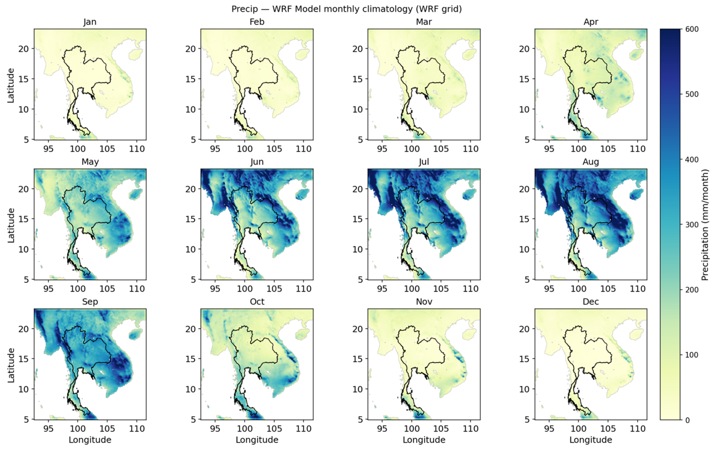
The monthly precipitation (Precip) climatology of Thailand is shown in Figure 2., highlighting the pronounced seasonal cycle characteristics of the monsoon climate. Observations from the CRU (top panels) indicate very low rainfall during the dry season (December–February), followed by a gradual increase during the pre-monsoon months (March–May). Peak precipitation occurs during the southwest monsoon (June–September), with spatial maxima along the western coastal regions and northern highlands, often exceeding 400 mm/month. Rainfall declines rapidly during the post-monsoon months (October–November), returning to dry conditions. The WRF simulation (bottom panels) captured the timing and general spatial distribution of the seasonal cycle. However, the model consistently produces higher rainfall totals during the monsoon season, particularly in orographically influenced regions, which reflects a systematic wet bias. Despite these biases, downscaling improves the representation of spatial gradients compared to the coarse observational grid, offering finer-scale detail that is important for regional climate impact assessment. Taken together, these results suggest that WRF downscaling improves the representation of precipitation patterns compared with the observed (CRU), but notable regional biases remain, especially in mountainous regions and in the simulation of extreme rainfall intensity.
Figure 2. Monthly precipitation climatology over Thailand from CRU observations (top, CRU grid) and WRF simulations (bottom, WRF grid) during the baseline period. Both datasets captured the seasonal cycle with peak rainfall during June–September and minima in December–February, although WRF tended to simulate higher rainfall intensities, particularly in orographic regions.
A spatial comparison between the modeled and observed precipitation climatology is presented in Figure 2. During the dry season, the model successfully reproduced the observed spatial patterns of low precipitation across most of the country. Both the WRF-CESM and CRU data showed minimal rainfall in the northern, northeastern, and central regions. The model also correctly captured the presence of precipitation in the southern peninsular region during this period. As the Southwest monsoon onset in mid-May, the model correctly simulated the increase in rainfall across the country. However, from June to September, a systematic wet bias became spatially evident. The model consistently overestimated the intensity and spatial extent of monsoon precipitation. The dark blue shades, representing heavy rainfall (>400 mm/month), covered a significantly larger area in the model output than in the CRU observations, particularly over northern Thailand and the broader Indochina peninsula. Although the magnitude is often incorrect, the model does capture key features of the spatial distribution, such as the localization of the heaviest rainfall along the windward slopes of the southwest coast region owing to the orographic effects.
The most significant model error occurred during the monsoon withdrawal period, particularly in October and November. The CRU observational data clearly show a distinct precipitation maximum along the southeast coast, driven by the onset of the Northeast Monsoon. However, the model failed to reproduce this critical feature. In summary, the model reproduces large-scale seasonal shifts in precipitation patterns but suffers from a significant wet bias during the summer monsoon and critically fails to simulate the autumn precipitation maximum in southeast coast Thailand.
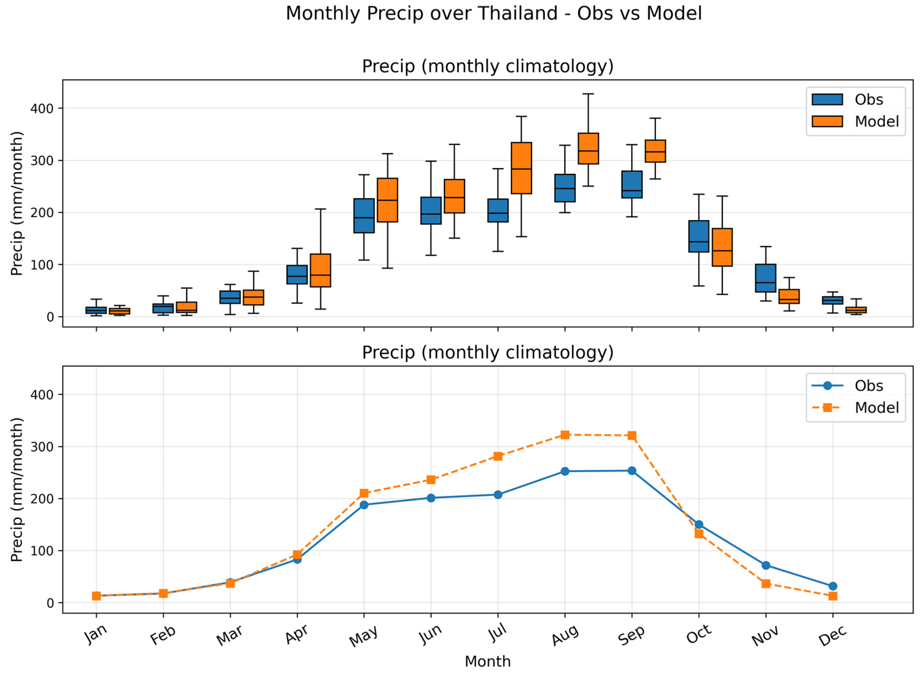
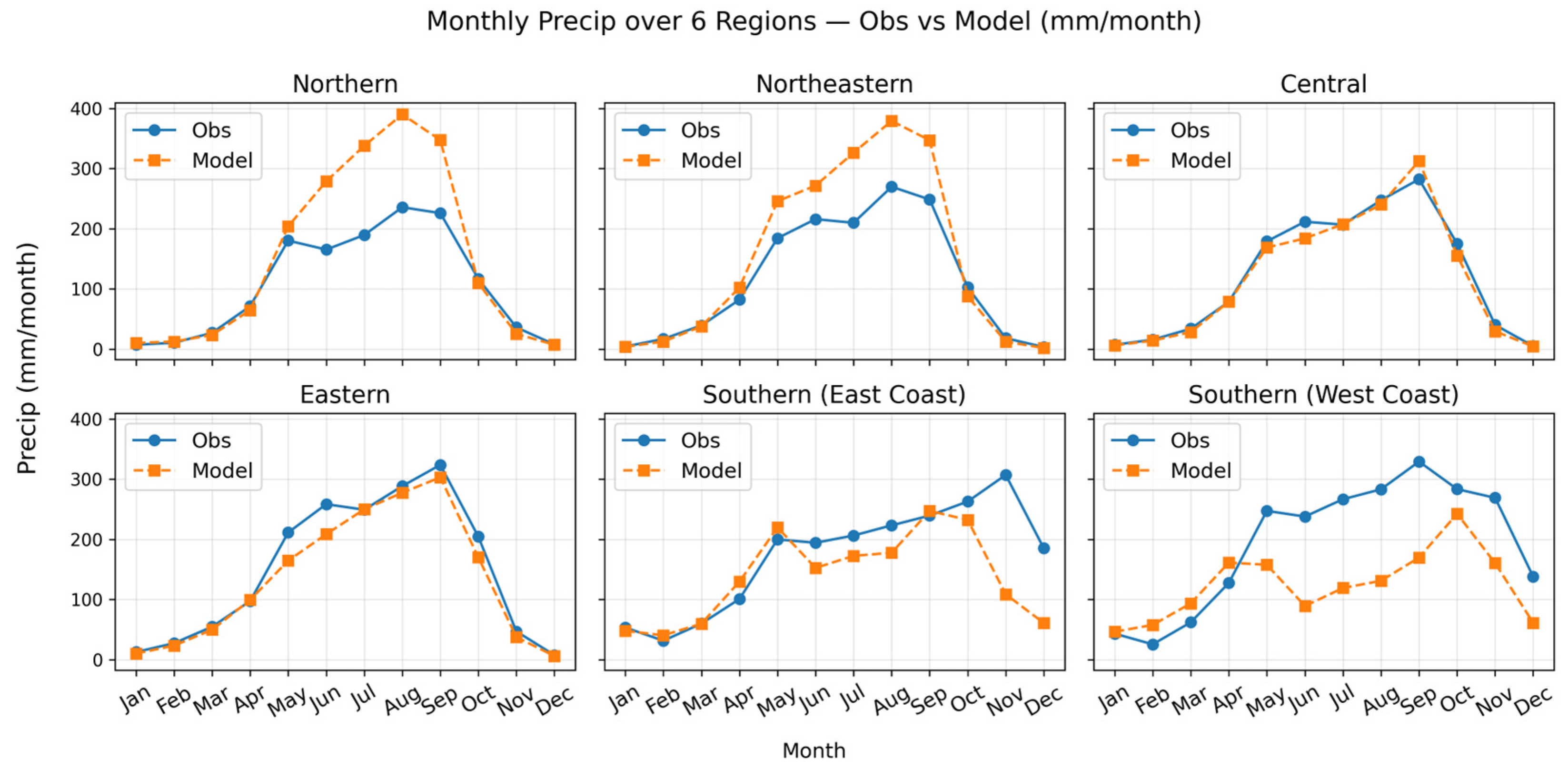
A comparison of observed and simulated monthly precipitation (Figure 3) indicates that the seasonal cycle of precipitation is well represented in WRF, with dry conditions during December–February, a rapid increase in rainfall during the pre-monsoon and early monsoon (April–June), peak rainfall in August–September, and a sharp decline in October–November. At the national scale, WRF tended to overestimate rainfall during the monsoon season by 50–100 mm/month, particularly from July to September, which is consistent with the wet bias noted in the spatial maps. Regionally, the strongest overestimations occurred in the northern and northeastern regions during the peak monsoon months, whereas the central and eastern regions showed moderate wet biases. In contrast, rainfall in the southern (east and west coasts) region was better simulated, with the model capturing the bimodal seasonal pattern, although with a slight overestimation in the southwest monsoon months. Overall, the WRF reproduced the timing and phasing of the seasonal precipitation cycle across Thailand but with a tendency to over-intensify monsoonal rainfall, especially in topographically influenced regions. The wet bias observed in the WRF simulations, particularly over mountainous regions, may partly arise from the sparse distribution of observed stations used in the CRU TS dataset []. Limited station coverage in areas with high rainfall introduces greater interpolation uncertainty, meaning part of the apparent overestimation likely reflects observational gaps rather than model error.
Figure 3. Comparison of observed (CRU) and simulated (WRF) monthly precipitation (mm/month) for the baseline period. (Top) Boxplots of monthly precipitation in Thailand. (Middle) National climatological mean monthly precipitation. (Bottom) Regional climatological cycles for the six administrative regions of Thailand.
The model’s simulation of monthly precipitation was evaluated against observational data, and its performance at the national and regional scales is presented in Figure 3. At the national level, the model’s primary systematic error was a significant overestimation of precipitation during the peak monsoon season. A pronounced positive (wet) bias was evident from May to September, as illustrated in the monthly climatology plot. Although the model correctly reproduces the annual rainfall phenology by distinguishing the dry season from the wet season and capturing the timing of the monsoon peak in August/September, it consistently simulates higher rainfall totals than those observed during these months. The monthly distribution in the top panel further confirms that the median and variance of the modeled precipitation exceeded the observations during this period.
The analysis of sub-regions revealed that this wet bias is a widespread characteristic, although the spatiotemporal performance of the model varies. In the northern, northeastern, central, eastern, and southern (east and west coast) regions, the model consistently overestimated the monsoon rainfall. The temporal pattern of the rainfall cycle was generally well captured, but the magnitude was too high. A more significant model deficiency was apparent in the southeast coast region, which has a distinct autumnal rainfall maximum. The model failed to reproduce this regional climate feature. It imposes a wet bias during the summer months (May–August), which is typical of other regions, and substantially underestimates the observed precipitation peak in October and November.
In summary, the model reproduces the general timing of the Thai monsoon but is characterized by a pervasive wet bias during the summer months and fails to accurately simulate the unique autumn-dominant precipitation regime on the southeast coast.
In terms of spatial and seasonal patterns (Figure 4), the model exhibited a systematic wet bias during the core monsoon months (June–September), particularly over northern, western, and central Thailand, where the simulated rainfall exceeded the observations by more than 75 mm/month. This tendency suggests an over-intensification of the orographic and convective rainfall processes in WRF. Conversely, during the dry season (December–February), the biases were smaller and more spatially heterogeneous, with localized overestimations in southern Thailand and slight underestimations in the northeast. During the pre-monsoon (March–May) and post-monsoon (October–November) transition seasons, the model showed mixed biases, with overestimations in the western and northern regions, coupled with underestimations in the northeast and along the coastal zones. Overall, these patterns highlight the WRF’s capability to capture the seasonal cycle but also its propensity to exaggerate rainfall during peak monsoon months, a common feature in high-resolution regional climate simulations.
Figure 4. Mean monthly precipitation bias (WRF–CRU, mm/month) for the baseline period shown on the CRU grid. Positive values (blue) indicate WRF overestimation, whereas negative values (red) indicate underestimation.

3.1.2. Precipitation Distributional Analysis

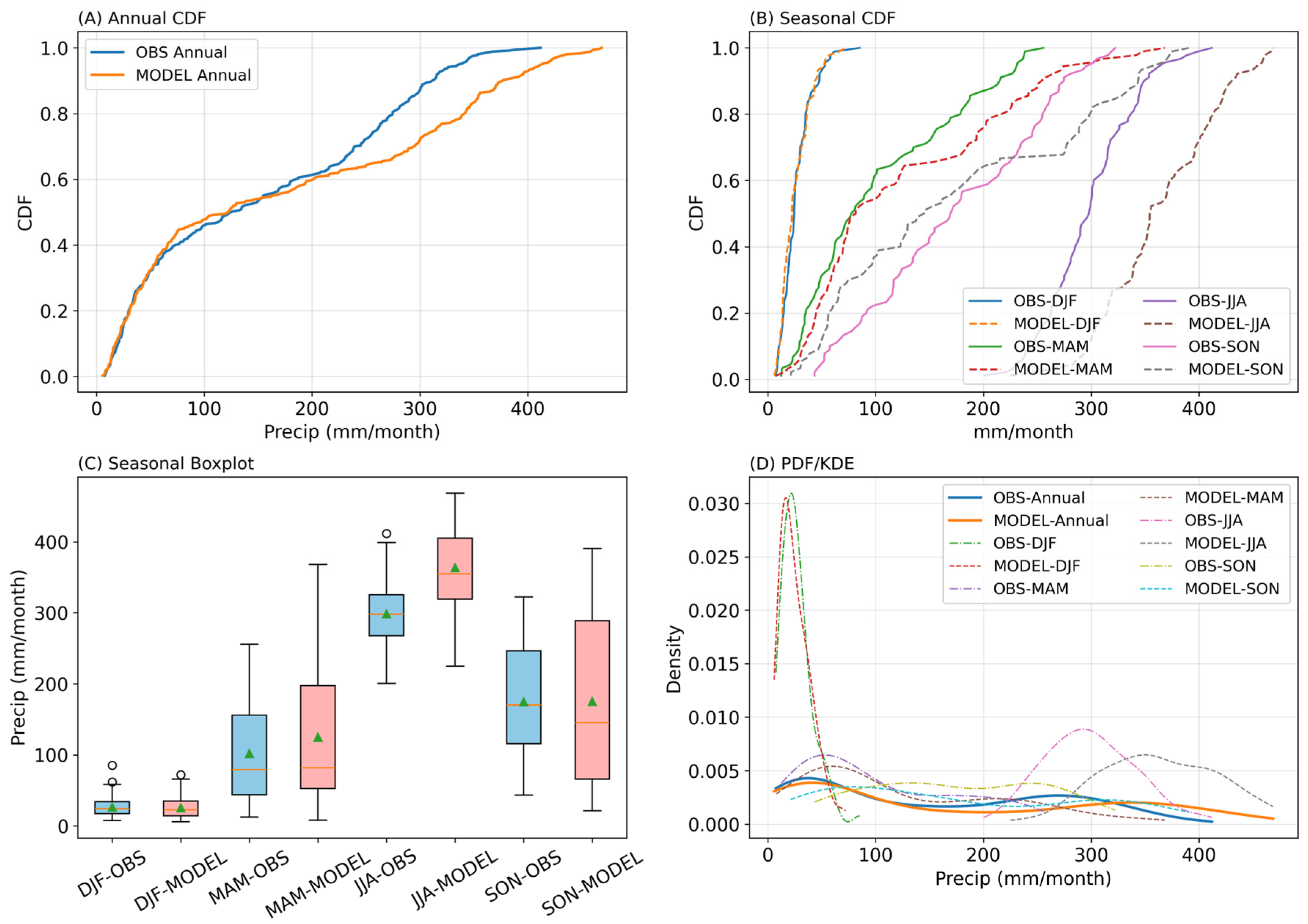
A comparison between the simulated and observed precipitation from 1976 to 2005 revealed systematic biases in the WRF-downscaled CMIP5 simulation (Figure 5 and Table 2). At the annual scale, the model produced a mean precipitation of 172 mm/month compared to 151 mm/month from CRU TS, corresponding to a wet bias of +22 mm/month (+14.5%). The annual distributions differed significantly, as confirmed by the KS test (D = 0.17, p < 0.001).
Figure 5. Cumulative distribution functions (CDFs), seasonal boxplots, and probability density functions (PDF/KDE) comparing simulated (MODEL) and observed (OBS; CRU TS) precipitation from 1976 to 2005.
Table 2. Statistical evaluation of annual and seasonal precipitation (mm) between observations and model simulations.
Seasonal analyses highlighted stronger discrepancies. In DJF, precipitation was very low in both observations and simulations, with the model slightly underestimating the mean (−1.1 mm/month, −4%), and the KS test showed no significant difference (p = 0.49). In contrast, MAM exhibited a moderate wet bias of +23 mm/month (+23%), although the difference in distribution was not statistically significant (p = 0.28). The most pronounced error occurred in JJA, where the model simulated a mean of 364 mm/month compared to 298 mm/month in the observations, representing an overestimation of +65 mm/month (+22%). The KS test indicated a highly significant difference in distribution (D = 0.51, p < 0.001). For SON, the model and observations had nearly identical means (175 mm/month), but differences in distribution shape were still evident (D = 0.23, p = 0.012).
Overall, these results demonstrate that the model tends to overestimate precipitation, particularly during the wet monsoon season (JJA). The overestimation manifested not only as higher mean rainfall but also as broader variability, as reflected in the seasonal boxplots and probability density functions. This systematic wet bias in the JJA represents a key limitation of the simulation and has implications for downstream impact assessments that rely on these precipitation fields.

3.2. Temperature Evaluation

3.2.1. Spatial and Temporal Maximum Temperature Characteristics

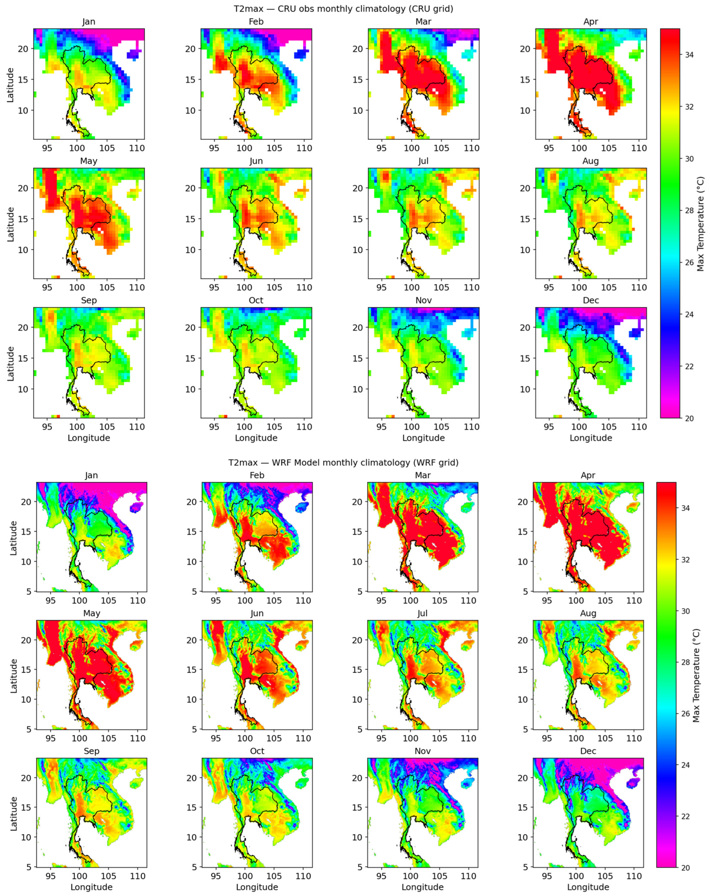
A spatial comparison between the modeled and observed (CRU) monthly maximum temperature (“T2max”) climatology is shown in Figure 6. The model successfully reproduced the large-scale spatial and temporal patterns of the annual T2max cycle. It correctly identified the location of the most intense heat during the pre-monsoon hot season (March–May), which is centered over the inland continental regions of Thailand and its neighbors. Similarly, the model captured the southward progression of cooler temperatures during the cool season (November–January). Despite accurately simulating general patterns, the model exhibited significant seasonal and spatial biases. Warm Bias (Hot Season) from March to May, the model overestimates the intensity and spatial extent of the heat. The areas shown in red (indicating T2max > 34 °C) were noticeably larger and more intense in the model output than in the CRU observations, confirming a warm bias during the peak hot season. Cold Bias (Monsoon and Cool Season) from June through February, the model displays a persistent cold bias. This is particularly evident from November to January, when the cool temperatures (blue and purple shades) cover a substantially larger geographical area and are more intense in the model simulation than in the observations. This indicates that the model overestimated cooling during the post-monsoon and cool seasons. In summary, the model accurately simulated the location and timing of seasonal temperature variations but was characterized by a distinct seasonal bias, exaggerating the peak heat of the hot season and the cooling of the monsoon and cool seasons.
Figure 6. Monthly maximum temperature climatology (°C) over Thailand from CRU observations (top, CRU grid) and WRF simulations (bottom, WRF grid) for the 1976–2005 baseline period.
Observations from the CRU showed clear seasonal and spatial gradients in the maximum temperature. Peak values occur during the pre-monsoon months (March–May), exceeding 34 °C across much of central and northeastern Thailand, whereas cooler conditions dominate the monsoon and post-monsoon months (June–October), particularly in the northern highlands. The coolest temperatures were observed during December–January, especially in the northern mountainous regions, where maxima fell below 24 °C.
The WRF simulation reproduced the broad seasonal cycle, with warm pre-monsoon conditions and cooler temperatures during the rainy and winter seasons. However, WRF exhibited systematic warm biases across most regions, especially in March–May, where the simulated maxima exceeded the CRU values by 1–3 °C. The model captures topographic cooling in mountainous zones, but the gradients are sharper and more spatially detailed than those in the coarser observational dataset. Overall, WRF provided an improved spatial representation of temperature features, although with a tendency to overestimate maximum temperatures during the hot season.
The evaluation of the modeled monthly mean maximum temperature (T2max) indicates that the WRF simulation effectively captures the national and regional patterns of the annual temperature cycle across Thailand (Figure 7). The model reproduces the timing and magnitude of seasonal temperature variations, with realistic warm peaks preceding the monsoon onset and cooler conditions during the wet season, although minor regional biases remain. The middle plot shows that the model correctly captured the timing of the annual temperature peak in April. However, the simulation exhibited a clear and systematic seasonal bias compared to the observations. A warm bias was evident from January to May, during which the model consistently overestimated the monthly mean T2max values. Conversely, a cold bias was observed for the remainder of the year (June to December). This underestimation was most pronounced at the end of the year, particularly in December. The boxplot in the top panel corroborates these findings, illustrating that the model’s monthly median and interquartile range are consistently higher than the observations in the first part of the year and lower in the second half.
Figure 7. Comparison of observed (CRU) and simulated (WRF) maximum temperatures (°C) for the baseline period. (Top) Boxplots of monthly T2max across Thailand. (Middle) National climatological mean monthly T2max. (Bottom) Regional climatological cycles for the six administrative regions of Thailand.
The regional analysis, presented in the six lower panels, indicates that the seasonal bias identified at the national level is a persistent feature across all Thailand’s subdomains. In the northern, northeastern, central, and eastern regions, the model accurately simulated the magnitude and timing of the sharp temperature maximum in April. Nevertheless, the subsequent cold bias was consistently present from approximately June to December in all four regions. For the southeast and southwest coast regions, which are characterized by a more moderate annual temperature range, the model reproduced the general cycle. However, the tendency towards underestimation in the latter half of the year remains a consistent feature. In summary, the results indicate that while the model can simulate the timing of the seasonal T2max cycle across Thailand, it is characterized by a systematic bias. The model overestimated the temperatures during the pre-monsoon hot season and consistently underestimated them throughout the monsoon and post-monsoon periods.
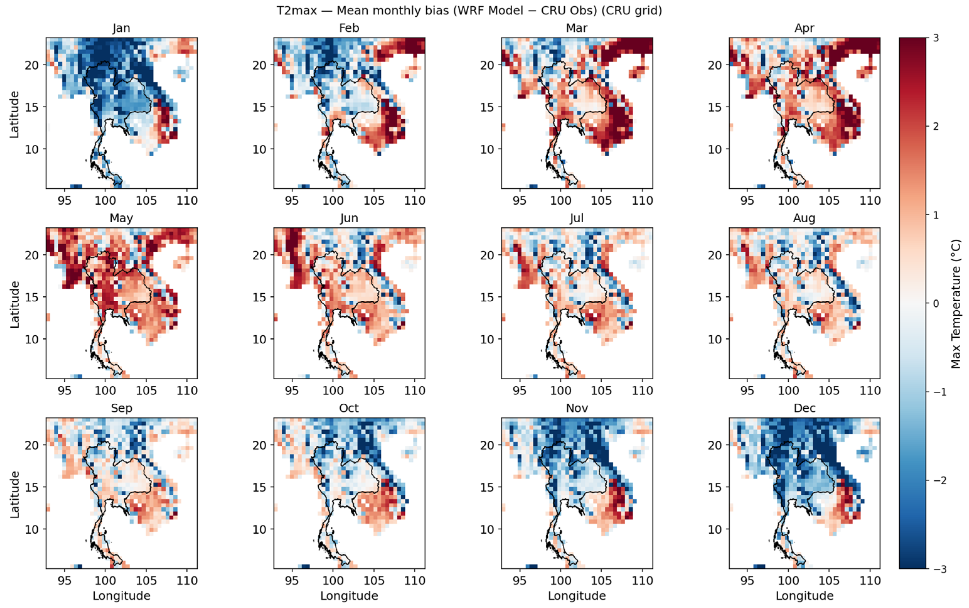
The bias patterns revealed distinct seasonal variations (Figure 8). During the cool season (December–February), the WRF tended to underestimate the maximum temperature by up to −2 to −3 °C across northern and northeastern Thailand, with localized warm biases in the coastal and southern regions. In contrast, the pre-monsoon hot season (March–May) exhibited systematic warm biases of +1 to +3 °C across much of central, northern, and northeastern Thailand, coinciding with the period of highest observed temperatures. During the monsoon months (June–September), warm biases persisted, particularly over the north and central plains, although with a smaller magnitude (approximately +1 °C), whereas localized cool biases appeared in the highland and coastal zones. In the post-monsoon transition (October–November), the WRF again underestimates the maximum temperature in the northern regions, indicating a seasonal shift in the bias structure. Overall, the model tended to overestimate heat during the pre-monsoon and underestimate cool-season temperatures, suggesting limitations in simulating surface energy balance and land–atmosphere interactions.
Figure 8. Mean monthly bias of maximum temperature (WRF–CRU, °C) for the 1976–2005 baseline period, shown on the CRU grid. Positive values (red) indicate WRF overestimation (warm bias), whereas negative values (blue) indicate underestimation (cold bias).

3.2.2. Maximum Temperature Distributional Analysis

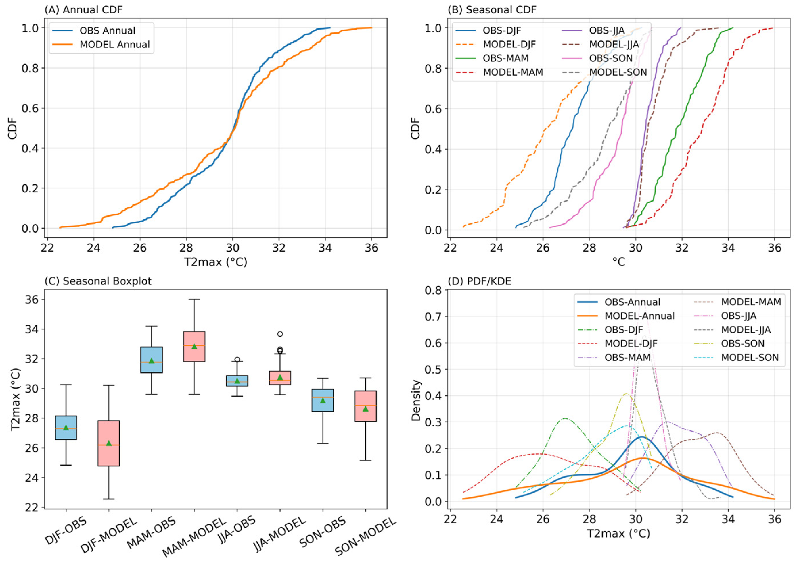
The evaluation of near-surface maximum temperature (T2max) during 1976–2005 showed that the model captured the broad annual distribution well, with a negligible annual mean bias of −0.09 °C (−0.3%) relative to CRU TS observations (Figure 9 and Table 3). Nevertheless, the Kolmogorov–Smirnov test indicated significant differences in the annual distributions (D = 0.11, p = 0.034), suggesting that the model tended to simulate a broader variance than the observations. Seasonal analyses revealed more pronounced biases. In DJF, the model exhibited a systematic cold bias of approximately −1.0 °C (−3.8%), which was highly significant (D = 0.37, p < 0.001). Conversely, in MAM, the model showed a warm bias of +0.95 °C (+3.0%), which was also statistically significant (D = 0.31, p < 0.001). During JJA, the bias was minimal (+0.24 °C, +0.8%), with no significant difference in distribution (p = 0.21). For SON, the model slightly underestimated the maximum temperature (−0.53 °C, −1.8%), with marginal statistical significance (D = 0.20, p = 0.047).
Figure 9. Cumulative distribution functions (CDFs), seasonal boxplots, and probability density functions (PDF/KDE) comparing simulated (MODEL) and observed (OBS; CRU TS) maximum temperature (T2max) during 1976–2005.
Table 3. Statistical evaluation of annual and seasonal maximum temperature (°C) between observations and model simulations.
These results are consistent with the seasonal boxplots and PDF/KDE analyses. The model distributions exhibited greater variability than the observations, particularly in DJF and MAM, where the biases were most pronounced. In contrast, JJA and SON were relatively well captured, with simulated means and variability closely aligned with observations. Overall, the model successfully reproduced the annual mean maximum temperature but showed a systematic cold bias in DJF and a warm bias in MAM, while JJA and SON were better represented. These contrasting seasonal errors suggest that model parameterizations and boundary conditions may need to be refined to better capture extremes across different climatic regimes.

3.2.3. Spatial and Temporal Minimum Temperature Characteristics

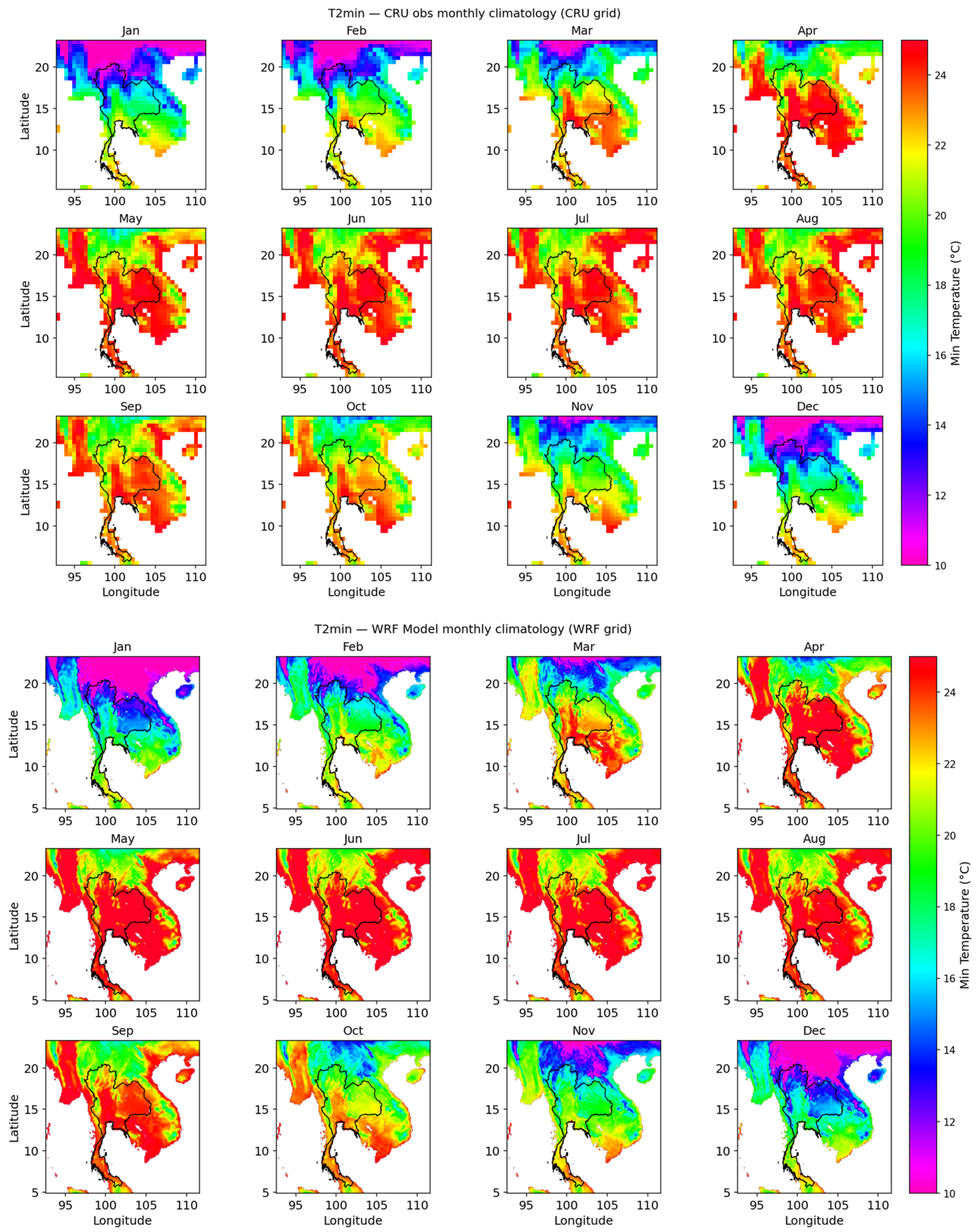
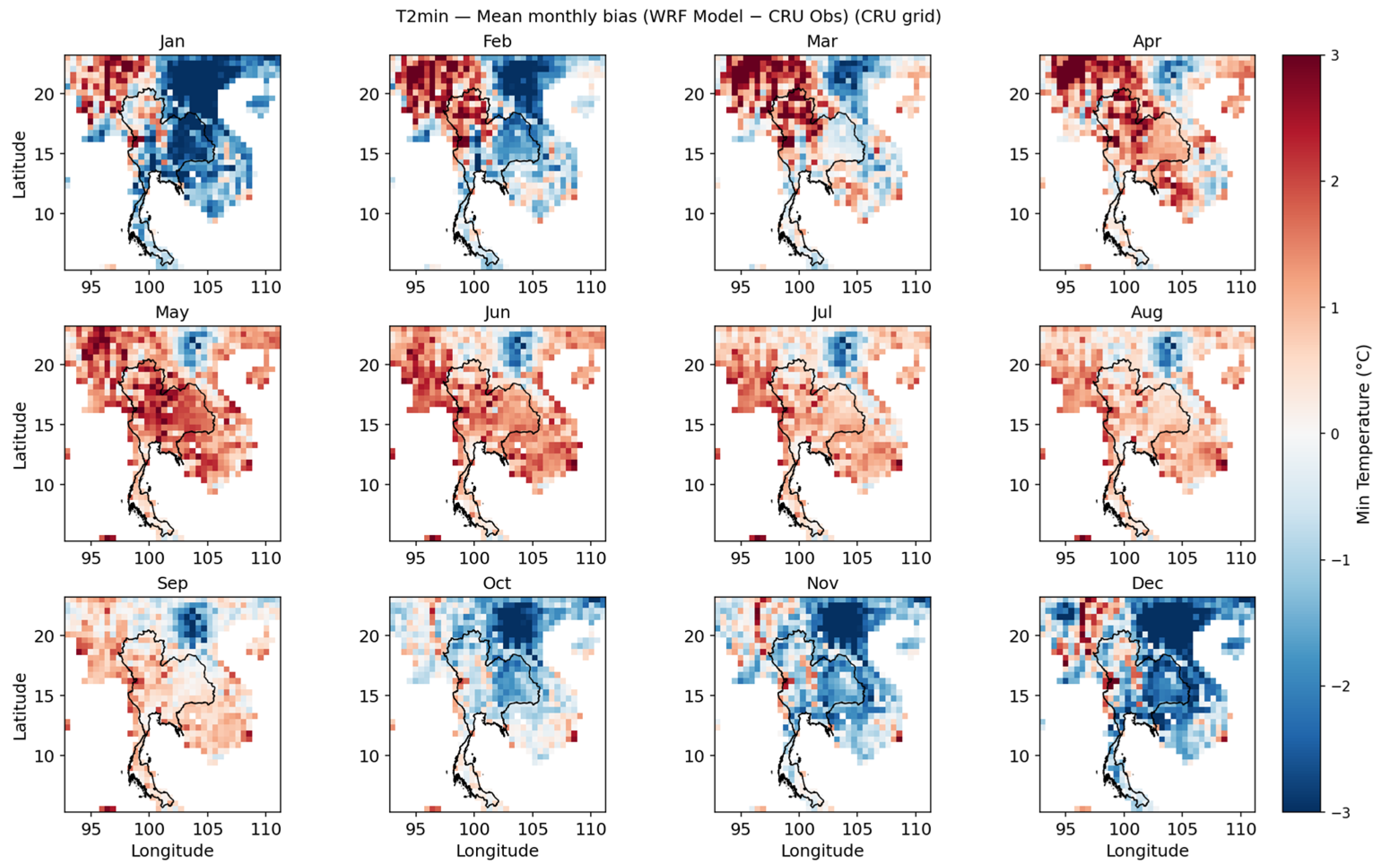
The CRU-observed minimum temperature data (Figure 10) indicated strong seasonal variation in minimum temperatures, with the coolest conditions during December–January (<14 °C across the northern highlands and <18 °C in the central and northeastern plains) and warmest values during April–May (>22 °C across most regions). Spatial gradients are largely controlled by topography; mountainous areas in the north and west consistently exhibit lower minimum temperatures, whereas low-lying regions, particularly the central plains and southern peninsula, remain warmer throughout the year. The WRF simulation (Figure 10) captured the seasonal cycle and spatial distribution of the minimum temperature, including the influence of elevation. However, the model consistently produced higher nighttime temperatures than CRU, particularly during the warm season (March–May) and monsoon (June–September), where WRF minimum temperatures exceeded 22 °C across much of the domain. This warm bias is evident across both lowland and upland regions, suggesting limitations in the WRF’s representation of nocturnal cooling processes and land–surface exchanges. Nevertheless, the model enhances spatial detail relative to coarser observational datasets, especially in complex terrain.
Figure 10. Monthly minimum temperature climatology (°C) over Thailand from CRU observations (top, CRU grid) and WRF simulations (bottom, WRF grid) for the baseline period.
The evaluation of the simulated monthly minimum temperature (T2min) against CRU observations (Figure 11 and Figure 12) shows that the WRF–CESM effectively reproduces the overall seasonal pattern and spatial distribution of temperature across Thailand, with minor regional deviations in magnitude. The comparison highlights the WRF’s ability to reproduce the observed seasonal cycle of T2min, with lowest values in December–January (16–18 °C) and highest values in April–May (24–25 °C). However, systematic biases were evident. At the national scale, WRF tended to overestimate T2min during the hot season (March–May) by 1–2 °C, while underestimating it during the cool season (November–January) by 1 °C. Regionally, warm biases were most pronounced in the central and northeastern regions during April–May, whereas cold biases were dominant in the northern region during December–January. The southern regions (east and west coasts) were generally better captured, although the WRF tended to simulate slightly warmer T2min throughout the year. Overall, the model captures the phasing of seasonal cycles but with consistent seasonal shifts: too warm during the pre-monsoon months and too cool in the cool season.
Figure 11. Comparison of observed (CRU) and simulated (WRF) minimum temperature (°C) for the 1976–2005 baseline period. (Top) Boxplots of monthly T2min in Thailand. (Middle) National climatological mean monthly T2min. (Bottom) Regional climatological cycles for the six administrative regions of Thailand.
Figure 12. Mean monthly bias of minimum temperature (WRF–CRU, °C) for the 1976–2005 baseline period, shown on the CRU grid. Positive values (red) indicate WRF overestimation (warm bias), whereas negative values (blue) indicate underestimation (cold bias).

3.2.4. Minimum Temperature Distributional Analysis

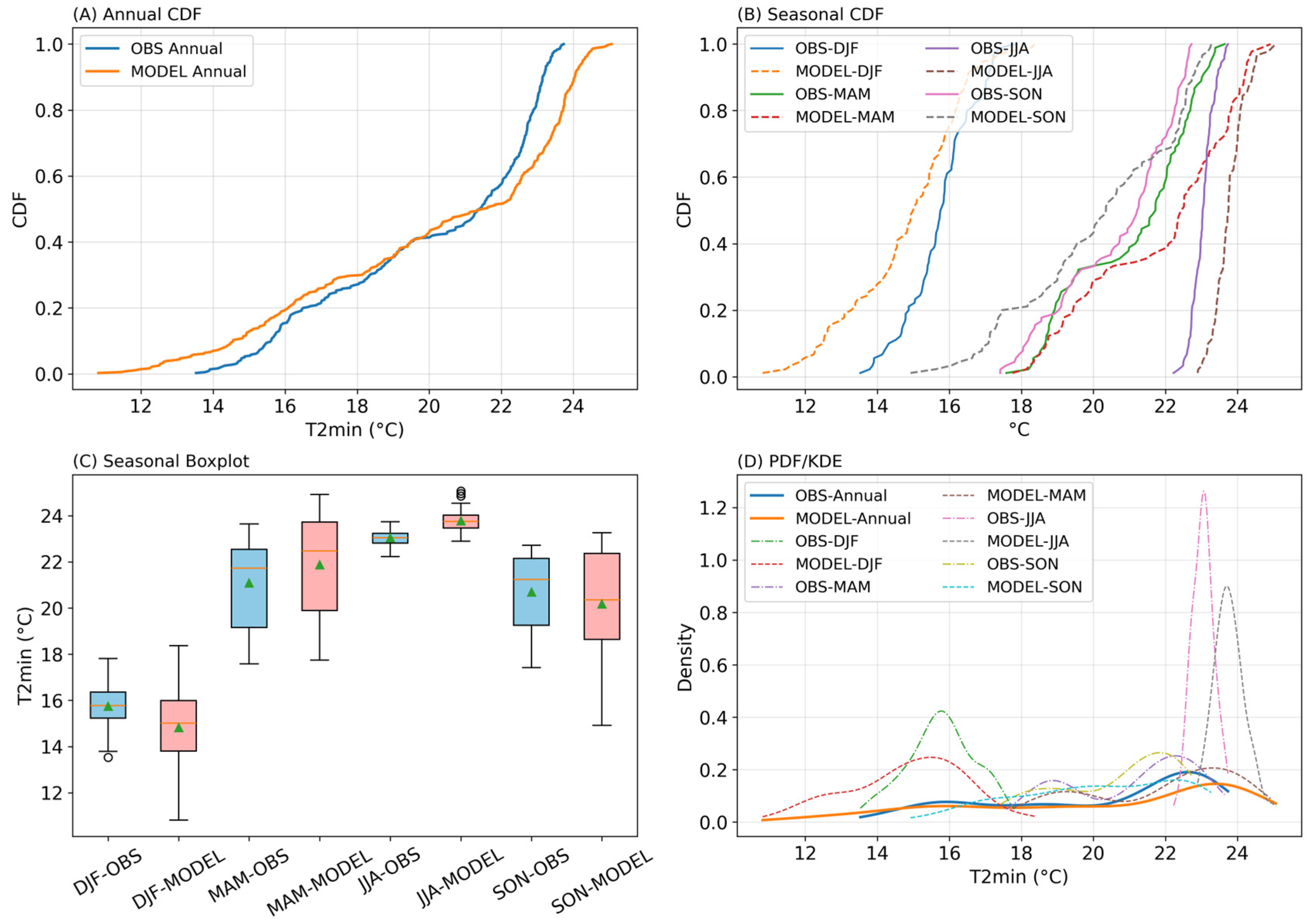
The evaluation of the near-surface minimum temperature (T2min) for the period 1976–2005 indicated that the model successfully reproduced the annual mean, with only a negligible bias of +0.02 °C (+0.1%) relative to the CRU TS observations (Figure 13 and Table 4). Nevertheless, the annual distributions differed significantly according to the KS test (D = 0.25, p < 0.001), reflecting an overestimation of interannual variability in the simulation.
Figure 13. Cumulative distribution functions (CDFs), seasonal boxplots, and probability density functions (PDF/KDE) comparing simulated (MODEL) and observed (OBS; CRU TS) minimum temperatures (T2min) from 1976 to 2005.
Table 4. Statistical evaluation of annual and seasonal minimum temperature (°C) between observations and model simulations.
Seasonal assessments revealed stronger discrepancies. During the DJF, the model exhibited a pronounced cold bias of −0.92 °C (−5.9%), with significant differences in distribution (D = 0.30, p < 0.001). In MAM, the model shifted to a warm bias of +0.79 °C (+3.7%), again statistically significant (D = 0.30, p < 0.001). The largest deviation occurred in JJA, where the model overestimated the minimum temperature by +0.74 °C (+3.2%), and the KS statistic indicated a highly significant difference (D = 0.70, p < 0.001). In contrast, the SON showed only a modest cold bias (−0.51 °C, −2.5%), with no statistically significant difference in distribution (p = 0.10).
These patterns are consistent with the seasonal boxplots and PDF/KDE analyses, which revealed that the model produced broader distributions than the observations, particularly in JJA. Overall, while the model reproduces the annual mean T2min, it shows a systematic cold bias in DJF and SON, a warm bias in MAM, and the largest positive bias in JJA, underscoring the limitations of simulating nighttime temperatures and seasonal variability.

3.3. Model Performance Metrics

A synthesis of the statistical evaluation of precipitation and temperature is presented in Table 5. The performance was assessed using the mean bias (MB), root mean square error (RMSE), and Pearson’s correlation coefficient (r) for the baseline period of 1976–2005. For precipitation, the WRF-downscaled CESM simulations exhibited a Thailand boundary mean bias (MBE) of +17.14 mm/month and an RMSE of 63.88 mm/month. The correlation with the CRU TS4.09 anomalies was r = 0.88, indicating a high skill in capturing interannual variability. Despite improvements relative to the raw CESM outputs, wet biases persisted over the northern and northeastern regions, and dry biases were observed in the central, eastern, and southern regions. For temperature, the Thailand-boundary MBEs of T2max and T2min were −1.25 °C and −0.80 °C, respectively, with RMSE values of 1.99 °C, 1.76 °C, and a correlation of r = 0.83, and r − 0.91. The downscaling substantially improved the spatial gradients and seasonal cycles compared with those of the driving CESM data. Overall, the downscaled simulations reduced systematic errors and improved the correlation with observations, particularly for temperature. However, precipitation simulations still exhibited notable regional biases, highlighting the sensitivity of downscaling performance to physical parameterizations and monsoon dynamics. The quantitative evaluation of the performance of the WRF-CESM against the CRU observational dataset for monthly precipitation, maximum temperature, and minimum temperature is presented in Table 2, Table 3 and Table 4.
Table 5. WRF-CESM performance against CRU grid observed for Thailand and TMD regions.

3.3.1. Temperature Performance

The model demonstrated high fidelity in simulating both the maximum and minimum temperatures, as evidenced by the strong correlation statistics. For maximum temperature (T2max), the temporal correlation coefficient (r) generally exceeded 0.80, except in the southern regions, and the Pattern Correlation Coefficient (PCC) was exceptionally high, peaking at 0.96 for the central region. Despite these strong correlations, a systematic negative Mean Bias Error (MBE) indicates a persistent cold bias of approximately −1.0 to −1.5 °C across all regions. For the minimum temperature (T2min), the model also exhibited excellent temporal and spatial correlations, with r and PCC values frequently exceeding 0.90, except in the southern regions. However, the reported MBE values in Table 5, which suggest a slight cold bias, are in direct contradiction to the pronounced warm bias identified in the graphical and spatial analyses. This discrepancy suggests a potential systematic error in the reported T2min bias statistics.

3.3.2. Precipitation Performance

The model performance for precipitation was considerably lower and more heterogeneous than that for temperature. The error metrics (MAE and RMSE) were an order of magnitude larger, indicating substantial deviations from the observations. The RMSE was particularly high in the southern regions, reaching 129.62 mm/month on the southwest coast and 102.25 mm/month on the southeast coast. The annual MBE revealed a distinct regional dipole: a positive bias (wet bias) was present in the northern (+44.79 mm/month) and northeastern (+36.06 mm/month) regions, whereas a negative bias (dry bias) was observed in the central, eastern, southeastern, and southwestern regions, with the largest negative bias in the southwest (−68.58 mm/month). The model’s skill was most deficient in the southern peninsula. The temporal correlation (r) degraded significantly to 0.49 (southeast) and 0.45 (southwest). Critically, the spatial pattern correlation for the southwest region was strongly negative (PCC = −0.89), signifying that the simulated spatial patterns were nearly an inversion of the observed patterns. The Kling–Gupta Efficiency (KGE) scores were also the lowest in this region, further confirming the poor performance of the model.
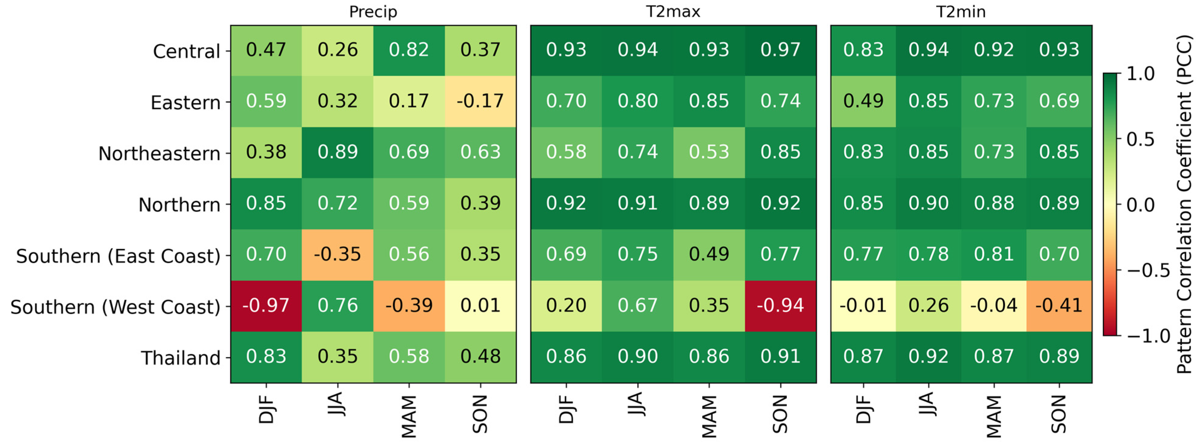
The results of the seasonal baseline analysis (1976–2005) for the WRF-CESM are presented in Figure 14, which displays the Pattern Correlation Coefficient (PCC) between the WRF-CESM output and CRU observational data for three key climate variables across various regions of Thailand. The model demonstrated high fidelity in simulating the spatial patterns of both maximum (T2max) and minimum (T2min) seasonal temperatures. As shown in the corresponding heatmaps, the PCC values were predominantly high and positive, frequently exceeding 0.80 across most regions and seasons. This indicates a strong agreement between the simulated and observed temperature patterns. However, a notable localized deficiency was observed in the southwestern coastal region. For T2max, the correlation was substantially weaker during the December–January–February (DJF) and March–April–May (MAM) seasons (PCC = 0.20 and 0.35, respectively). In contrast, the September–October–November (SON) season exhibited a strong negative correlation (PCC = –0.94), indicating that the WRF–CESM failed to capture the maximum temperature variability in the southwest coast region during this period. The model skill diminished further for T2min in the same region and seasons, where the PCC values were near zero or slightly negative (PCC = −0.01 for DJF, −0.04 for MAM, 0.26 for JJA, and −0.41 for SON), indicating a failure to reproduce the observed spatial patterns.
Figure 14. Pattern correlation coefficients (PCCs) between WRF and CESM baseline simulations (1976–2005) and CRU observations for precipitation (Precip), maximum temperature (T2max), and minimum temperature (T2min).
In contrast to temperature, the model’s performance in simulating precipitation was considerably more heterogeneous. The analysis revealed areas of both strong and weak performance, as well as significant negative correlations. High positive correlations were found in the northern region during JJA (PCC = 0.89), the northern region during DJF (PCC = 0.85), and the central region during MAM (PCC = 0.82), suggesting proficient simulation in these specific contexts. However, the model exhibits critical deficiencies in other areas. The most pronounced discrepancy occurred in the southwest coast region during the DJF season, which yielded a strong negative correlation (PCC = –0.97), indicating that the simulated precipitation patterns were nearly an inversion of the observed precipitation. Additional instances of poor performance included negative correlations in the southwest coast region during the MAM and JJA seasons (PCC = –0.97 and –0.39), in the southeast coast region during JJA (PCC = –0.35), and weak to negative correlations across multiple regions, such as in eastern Thailand from March to November (PCC ranging from –0.17 to 0.32).
In summary, the evaluation revealed that the WRF-CESM configuration was skillful at reproducing seasonal temperature patterns but exhibited significant, spatially dependent deficiencies in simulating seasonal precipitation.

4. Discussion

4.1. Added Value of WRF Downscaling for Thailand

The findings of this study highlight the significant added value of dynamical downscaling using the WRF model, particularly when compared with coarse-resolution CMIP5 simulations [,]. The WRF. Model accurately represents Thailand’s topographic and land use features, clearly distinguishing the mountainous North and West, the Central Plain, and the coastal lowlands. The elevation and land cover inputs effectively capture key surface characteristics, providing a strong physical basis for regional climate simulation. By explicitly resolving key local-scale processes such as topographic forcing, land–atmosphere interactions, and coastal contrasts, the WRF model provides a more physically realistic representation of precipitation and temperature across Thailand []. In Thailand, these improvements are particularly critical. Studies have shown that using appropriate model configurations, such as specific convective schemes with nudging, can substantially reduce rainfall biases relative to observations, thereby enhancing the reliability of regional climate projections [,]. This enhanced spatial detail is crucial for a nation to locally implement Thailand’s NAP for six climate-sensitive sectors such as agriculture, and water management. More accurate simulations enable stakeholders to better assess climate risks in the drought [], and flood prone areas. Furthermore, WRF has proven to be a powerful tool for urban and micro-climate studies; when coupled with urban canopy models (WRF-UCM), it can significantly improve simulations of neighborhood-scale climate phenomena such as the urban heat island effect [].
Ultimately, high-resolution downscaling represents an essential step in transforming large-scale climate projections into decision-relevant information that supports locally led adaptation action, resilience and sustainable development in Thailand []. Beyond Thailand, the benefits of WRF downscaling have been demonstrated in Southeast Asia and globally, particularly in regions with complex terrain and sparse observational networks [,]. The WRF consistently outperformed coarser global models by capturing fine-scale features that shape the local climate, including orographic effects, land–atmosphere interactions, and coastal gradients. Consequently, it provides more accurate simulations of precipitation, temperature, and extreme events, a capability well documented in topographically diverse regions such as the Tibetan Plateau, High Mountain Asia, and Central Asia [,,].

4.2. Systematic Biases and Their Implications

Despite the added value of dynamical downscaling, the persistence of systematic biases in WRF model simulations remains a significant challenge in this regard. These biases, which vary by region, season, and model configuration [], affect the reliability of the WRF outputs for both research and operational applications. A common issue is the overestimation of precipitation (wet bias), particularly during summer and in regions with complex terrain [,]. This bias is often attributed to the internal physics of the model, with the choice of parameterization schemes for convection and cloud micro-physics being the primary contributing factors [,].
In parallel, a cold bias is another frequently observed issue, especially in high-elevation areas such as the Tibetan Plateau, which can be linked to the misrepresentation of surface properties such as albedo []. It is crucial to recognize that these biases emerge from a multifaceted interplay of the model’s internal physics, including the planetary boundary layer (PBL) and land surface schemes, and are not solely inherited from the boundary conditions. These inherent model limitations have direct implications for applied studies, potentially affecting the accuracy of agricultural models and leading to exaggerated flood projections in highland catchments [].
Recognizing these challenges underscores the necessity of incorporating advanced bias-adjustment techniques as standard postprocessing steps [,]. Furthermore, developing multi-physics ensembles is a critical strategy for quantifying and bracketing the uncertainty arising from different model structures and parameterization choices [,]. Acknowledging and actively addressing these biases is essential for producing robust climate information to support reliable policy and adaptation decisions.

4.3. Relevance for Climate Adaptation and Resilience

The WRF model is a critical tool for translating coarse global climate projections into high-resolution regional-to-local data, which are essential for effective climate adaptation and resilience planning [,]. Dynamical downscaling with the WRF model adds significant value by capturing local climate features and extreme events that coarse Global Climate Models (GCMs) often miss [,]. By resolving fine-scale phenomena related to topography, land use, and urban environments, the WRF model provides a more physically plausible basis for assessing regional climate impacts. This enhanced regional-to-local detail is particularly crucial for improving the simulation of extreme events, such as heatwaves, hazardous convective weather, and tropical cyclones [,,]. These improved simulations are a primary driver of climate-related damage and are vital for designing resilient infrastructure and effective emergency response plans.
High-resolution datasets produced by WRF are used across numerous sectors to support targeted adaptation and mitigation strategies. For Water Resources, downscaled data improve precipitation and runoff modeling, especially in areas with complex terrain, leading to better water management strategies []. In Urban Planning and Public Health, WRF can generate hyper-local heat stress projections for cities, helping to inform public health interventions and urban design []. When coupled with chemistry models, such as CMAQ, the model provides valuable insights into climate–chemistry interactions, aiding in Air Quality management [].
Despite its strengths, dynamical downscaling using WRF faces several challenges. This process is computationally expensive, which can limit the size of the model ensembles and the quantification of uncertainty []. Furthermore, differences in downscaling methodologies and a lack of clear standards can lead to a range of projections, highlighting the need for careful comparison of datasets [,]. While WRF improves physical realism, model biases and choices in parameterization schemes can still affect the results []. Ongoing research is focused on addressing these issues. Hybrid and machine learning approaches have emerged to reduce computational costs while maintaining physical constraints [,,]. Overall, WRF-based climate downscaling is a cornerstone of regional climate adaptation, providing actionable high-resolution data that are becoming increasingly accessible and reliable for decision-makers.

4.4. Toward Future Climate Projections and Sustainable Development

The WRF model is a crucial tool for creating high-resolution regional climate projections that provide essential insights into sustainable development planning. By downscaling global climate scenarios, the WRF offers a more detailed and localized view of future climate change, which is fundamental for developing effective and targeted adaptation and mitigation strategies across various sectors []. WRF-based studies have consistently projected significant regional warming and altered precipitation patterns across the globe. Projections often indicate substantial warming in Europe and Asia [,]. Changes in precipitation are highly variable by region and season; for example, studies project significant drying and increased drought risk in Southern Europe, including Portugal and the Iberian Peninsula [,], whereas other areas in Asia, such as China and India, may experience increased mean rainfall [,]. Beyond shifts in the averages, high-resolution WRF simulations are particularly valuable for revealing future trends in extreme events. A key insight is the projected shift toward more intense and frequent extreme precipitation, which can occur even in regions where the average precipitation is expected to decrease, a finding with critical implications for future flood and drought risk management [,].
Detailed projections from WRF directly inform sustainable development by quantifying climate impacts. In agriculture, these projections help assess the impact on crop yields and inform adaptation strategies to ensure food security []. For urban planning and public health, the WRF can model future changes in urban heat stress and wind patterns, as seen in studies of China’s Pearl River Delta, providing vital information for designing resilient cities []. In terms of water resource management, the model supports robust planning for future water security by projecting changes in extreme rainfall and seasonal water availability in regions such as Western Canada []. Furthermore, these projections can be used to assess the future potential and variability of renewable energy sources, such as solar power in Greece, thereby aiding in long-term energy planning []. By providing region-specific insights, WRF modeling helps identify future risks and opportunities, making it an essential tool for developing targeted strategies to achieve sustainable development goals in a changing climate.

4.5. Uncertainties and Limitations

This study acknowledges several sources of uncertainty that may influence the interpretation of the results. First, the simulations were driven by a single GCM (CESM) and employed a single RCM configuration (WRF), which may not fully represent the range of potential climate variability or structural uncertainty associated with different model physics and boundary conditions. Using one model setup provides a controlled framework for baseline evaluation but limits the exploration of ensemble variability.
Second, the evaluation relied on a single observational dataset (CRU TS version 4.09), which, although globally recognized and quality-controlled, has a relatively coarse spatial resolution (0.5° × 0.5°, approximately 50 × 50 km). The CRU dataset was chosen because of its long-term temporal coverage, global consistency, and widespread use in CMIP5 and CORDEX–SEA evaluations, ensuring methodological comparability and regional relevance. To address the scale mismatch, all WRF–CESM outputs were bilinearly regridded to the CRU grid before analysis. This process preserves large-scale climatological patterns and facilitates consistent evaluation but inevitably smooths fine-scale features represented in the 12 km simulations.
Third, the use of CMIP5 boundary data instead of the more recent CMIP6 outputs introduces additional uncertainty. The CMIP5 dataset was selected because it provides bias-corrected boundary conditions that are directly compatible with the WRF Preprocessing System (WPS) and have been extensively validated in regional applications within the CORDEX–Southeast Asia framework. At the time of this study’s experimental design, bias-corrected CMIP6 datasets suitable for WRF had not yet been fully released or standardized for preprocessing. Nevertheless, CMIP6 offers updated forcings and improved physics, and future work will include CMIP6-driven simulations to assess the potential improvements and differences in the projected climate behavior.
These limitations may influence the magnitude and spatial distribution of model biases; however, the consistent patterns between simulated and observed climatology across multiple variables reinforce result robustness. Future research should extend this framework by incorporating multi-model ensembles (multiple GCM–RCM combinations) and higher-resolution observational or reanalysis datasets, such as ERA5, ERA5-Land, or APHRODITE, to better quantify structural and data-related uncertainties. Such improvements will enhance the confidence and applicability of high-resolution climate simulations for impact assessments and decision support in Thailand and Southeast Asia.

5. Conclusions

Dynamical downscaling with the Weather Research and Forecasting (WRF) model has emerged as a cornerstone for bridging the gap between coarse-resolution global climate models and the fine-scale information required for impact assessment and adaptation planning. The findings from both global and Thailand-focused studies confirm that WRF provides substantial added value by resolving complex terrain effects, land–atmosphere interactions, and localized climate processes that are otherwise overlooked in global models. These improvements are particularly crucial for climate-sensitive sectors as identified in Thailand’s NAP, including agriculture, water management, and disaster risk reduction, where reliable climate information is a prerequisite for informed decision-making and local action.
Nevertheless, systematic biases remain a persistent challenge, with precipitation overestimation and cold biases in high-elevation regions being the most prominent issues. Addressing these uncertainties through bias correction, multi-physics ensemble approaches, and integration with advanced statistical and machine learning techniques is essential to enhance the robustness of future projections. Recognizing and actively accounting for such limitations ensures that WRF outputs are both scientifically rigorous and operationally relevant.
The broader relevance of WRF downscaling lies in its contribution to climate resilience and sustainable development (SD). By offering high-resolution insights into regional climate variability and extremes, WRF empowers stakeholders to design context-specific adaptation strategies, from anticipating droughts in northeastern Thailand to mitigating urban heat stress in megacities. Furthermore, WRF-based projections of future warming and shifting precipitation regimes highlight the risks and opportunities for sustainable agriculture, water resource security, and renewable energy planning. In summary, despite the challenges, the continued advancement and application of WRF dynamical downscaling provide a pathway toward actionable high-resolution climate information. This capability is indispensable for supporting science-based policies and adaptation measures that align with national priorities and global sustainable development goals (SDGs).

Author Contributions

Conceptualization, C.C.; methodology, C.C.; software, C.C. and D.L.; validation, C.C. and D.L.; formal analysis, C.C. and D.L.; investigation, C.C. and D.L.; resources, C.C.; data curation, C.C.; writing—original draft preparation, C.C. and D.L.; writing—review and editing, C.C., D.L., A.L., K.T., S.N. and P.T.; visualization, C.C.; project administration, C.C.; funding acquisition, C.C. All authors have read and agreed to the published version of the manuscript.

Funding

This research was supported by the Thailand–China collaborative research project “Climate Change and Climate Variability Research in Monsoon Asia (CMON3)”, funded by the National Research Council of Thailand (NRCT), grant numbers N10A640315 and N10A650843, with partial support from Chiang Mai University (CMU).

Institutional Review Board Statement

Not applicable.

Data Availability Statement

The original contributions presented in this study are included in the article materials. Further inquiries should be directed to the corresponding authors.

Acknowledgments

The authors gratefully acknowledge the National Science Foundation (NSF) and NCAR Geoscience Data Exchange for providing access to the NCAR CESM global bias-corrected CMIP5 outputs. We also thank the Climatic Research Unit (CRU) for making their gridded observational datasets publicly available. In addition, we are indebted to the NCAR Mesoscale and Microscale Meteorology Laboratory for the development and continued maintenance of the WRF model, which was central to this study.

Conflicts of Interest

The authors declare no conflicts of interest.

References

  1. IPCC; Masson-Delmotte, V.; Zhai, P.; Pirani, A.; Connors, S.L.; Péan, C.; Berger, S.; Caud, N.; Chen, Y.; Goldfarb, L.; et al. Climate Change 2021: The Physical Science Basis. Contribution of Working Group I to the Sixth Assessment Report of the Intergovernmental Panel on Climate Change; Cambridge University Press: Cambridge, UK, 2021. [Google Scholar]
  2. Kamworapan, S.; Surussavadee, C. Evaluation of CMIP5 Global Climate Models for Simulating Climatological Temperature and Precipitation for Southeast Asia. Adv. Meteorol. 2019, 2019, 1067365. [Google Scholar] [CrossRef]
  3. Tangang, F.; Santisirisomboon, J.; Juneng, L.; Salimun, E.; Chung, J.; Supari, S.; Cruz, F.; Ngai, S.T.; Ngo-Duc, T.; Singhruck, P.; et al. Projected Future Changes in Mean Precipitation over Thailand Based on Multi-model Regional Climate Simulations of CORDEX Southeast Asia. Int. J. Climatol. 2019, 39, 5413–5436. [Google Scholar] [CrossRef]
  4. Maichandee, S.; Namwong, P.; Methakeson, O. Impacts of Climate Change and Regional Variations on Future Rainfall Patterns in Thailand by Downscaling Method. ASEAN J. Sci. Technol. Rep. 2023, 27, 80–91. [Google Scholar] [CrossRef]
  5. Kimmany, B.; Visessri, S.; Pech, P.; Ekkawatpanit, C. The Impact of Climate Change on Hydro-Meteorological Droughts in the Chao Phraya River Basin, Thailand. Water 2024, 16, 1023. [Google Scholar] [CrossRef]
  6. Masud, M.B.; Soni, P.; Shrestha, S.; Tripathi, N.K. Changes in Climate Extremes over North Thailand, 1960–2099. J. Climatol. 2016, 2016, 4289454. [Google Scholar] [CrossRef]
  7. Shrestha, S.; Lohpaisankrit, W. Flood Hazard Assessment under Climate Change Scenarios in the Yang River Basin, Thailand. Int. J. Sustain. Built Environ. 2017, 6, 285–298. [Google Scholar] [CrossRef]
  8. Kure, S.; Tebakari, T. Hydrological Impact of Regional Climate Change in the Chao Phraya River Basin, Thailand. Hydrol. Res. Lett. 2012, 6, 53–58. [Google Scholar] [CrossRef]
  9. Khampeera, A.; Yongchalermchai, C.; Techato, K. Drought Monitoring Using Drought Indices and Gis Techniques in Kuan Kreng Peat Swamp, Southern Thailand. Walailak J. Sci. Technol. 2018, 15, 357–370. [Google Scholar] [CrossRef]
  10. Homdee, T.; Pongput, K.; Kanae, S. A Comparative Performance Analysis of Three Standardized Climatic Drought Indices in the Chi River Basin, Thailand. Agric. Nat. Resour. 2016, 50, 211–219. [Google Scholar] [CrossRef]
  11. Taylor, K.E.; Stouffer, R.J.; Meehl, G.A. An Overview of CMIP5 and the Experiment Design. Bull. Am. Meteorol. Soc. 2012, 93, 485–498. [Google Scholar] [CrossRef]
  12. Pan, Z.; Zhang, Y.; Liu, X.; Gao, Z. Current and Future Precipitation Extremes over Mississippi and Yangtze River Basins as Simulated in CMIP5 Models. J. Earth Sci. 2016, 27, 22–36. [Google Scholar] [CrossRef]
  13. Chen, F.; Dudhia, J. Coupling and Advanced Land Surface-Hydrology Model with the Penn State-NCAR MM5 Modeling System. Part I: Model Implementation and Sensitivity. Mon. Weather Rev. 2001, 129, 569–585. [Google Scholar] [CrossRef]
  14. Sonali, P.; Nagesh Kumar, D. Review of Recent Advances in Climate Change Detection and Attribution Studies: A Large-Scale Hydroclimatological Perspective. J. Water Clim. Change 2020, 11, 1–29. [Google Scholar] [CrossRef]
  15. Zehr, S.C. Public Representations of Scientific Uncertainty about Global Climate Change. Public Underst. Sci. 2000, 9, 85. [Google Scholar] [CrossRef]
  16. Shen, M.; Chen, J.; Zhuan, M.; Chen, H.; Xu, C.Y.; Xiong, L. Estimating Uncertainty and Its Temporal Variation Related to Global Climate Models in Quantifying Climate Change Impacts on Hydrology. J. Hydrol. 2018, 556, 10–24. [Google Scholar] [CrossRef]
  17. Takayabu, I.; Ishizaki, N.N.; Nakaegawa, T.; Sasaki, H.; Wongseree, W. Potential of Representing the Diurnal Cycle of Local-Scale Precipitation in Northeastern Thailand Using 5-Km and 2-Km Grid Regional Climate Models. Hydrol. Res. Lett. 2021, 15, 1–8. [Google Scholar] [CrossRef]
  18. Hariadi, M.H.; van der Schrier, G.; Steeneveld, G.; Sopaheluwakan, A.; Tank, A.K.; Roberts, M.J.; Moine, M.; Bellucci, A.; Senan, R.; Tourigny, E.; et al. Evaluation of Onset, Cessation and Seasonal Precipitation of the Southeast Asia Rainy Season in CMIP5 Regional Climate Models and HighResMIP Global Climate Models. Int. J. Climatol. 2022, 42, 3007–3024. [Google Scholar] [CrossRef]
  19. Cruz, F.T.; Narisma, G.T.; Dado, J.B.; Singhruck, P.; Tangang, F.; Linarka, U.A.; Wati, T.; Juneng, L.; Phan-Van, T.; Ngo-Duc, T.; et al. Sensitivity of Temperature to Physical Parameterization Schemes of RegCM4 over the CORDEX-Southeast Asia Region. Int. J. Climatol. 2017, 37, 5139–5153. [Google Scholar] [CrossRef]
  20. Tangang, F.; Chung, J.X.; Juneng, L.; Supari; Salimun, E.; Ngai, S.T.; Jamaluddin, A.F.; Mohd, M.S.F.; Cruz, F.; Narisma, G.; et al. Projected Future Changes in Rainfall in Southeast Asia Based on CORDEX–SEA Multi-Model Simulations. Clim. Dyn. 2020, 55, 1247–1267. [Google Scholar] [CrossRef]
  21. Chotamonsak, C.; Salathé, E.P.; Kreasuwan, J.; Chantara, S.; Siriwitayakorn, K. Projected Climate Change over Southeast Asia Simulated Using a WRF Regional Climate Model. Atmos. Sci. Lett. 2011, 12, 213–219. [Google Scholar] [CrossRef]
  22. Ratna, S.; Ratnam, J.; Behera, S.; Tangang, F.; Yamagata, T. Validation of the WRF Regional Climate Model over the Subregions of Southeast Asia: Climatology and Interannual Variability. Clim. Res. 2017, 71, 263–280. [Google Scholar] [CrossRef]
  23. Saesong, T.; Ratjiranukool, P.; Ratjiranukool, S. Evaluation of Temperature Simulation over Northern Thailand from Regional Climate Model Coupled with Land Surface Model. Appl. Mech. Mater. 2017, 866, 108–111. [Google Scholar] [CrossRef]
  24. Ratjiranukool, P.; Ratjiranukool, S. Projection of Extreme Temperature over Northern Thailand by WRF Model. Appl. Mech. Mater. 2017, 866, 104–107. [Google Scholar] [CrossRef]
  25. Chhin, R.; Oeurng, C.; Yoden, S. Drought Projection in the Indochina Region Based on the Optimal Ensemble Subset of CMIP5 Models. Clim. Change 2020, 162, 687–705. [Google Scholar] [CrossRef]
  26. Nath, R.; Cui, X.; Nath, D.; Graf, H.F.; Chen, W.; Wang, L.; Gong, H.; Li, Q. CMIP5 Multimodel Projections of Extreme Weather Events in the Humid Subtropical Gangetic Plain Region of India. Earths Future 2017, 5, 224–239. [Google Scholar] [CrossRef]
  27. Zhang, Y.; You, Q.; Chen, C.; Ge, J.; Adnan, M. Evaluation of Downscaled CMIP5 Coupled with VIC Model for Flash Drought Simulation in a Humid Subtropical Basin, China. J. Clim. 2018, 31, 1075–1090. [Google Scholar] [CrossRef]
  28. Harding, K.J.; Snyder, P.K.; Liess, S. Use of Dynamical Downscaling to Improve the Simulation of Central U.S. Warm Season Precipitation in CMIP5 Models. J. Geophys. Res. Atmos. 2013, 118, 12-522–12-536. [Google Scholar] [CrossRef]
  29. Rojpratak, S.; Supharatid, S. Regional Extreme Precipitation Index: Evaluations and Projections from the Multi-Model Ensemble CMIP5 over Thailand. Weather Clim. Extrem. 2022, 37, 100475. [Google Scholar] [CrossRef]
  30. Supharatid, S.; Aribarg, T.; Supratid, S. Assessing Potential Flood Vulnerability to Climate Change by CMIP3 and CMIP5 Models: Case Study of the 2011 Thailand Great Flood. J. Water Clim. Change 2016, 7, 52–67. [Google Scholar] [CrossRef]
  31. De Silva, Y.K.; Babel, M.S.; Abatan, A.A.; Khadka, D.; Shanmugasundaram, J. Evaluation of ENSO in CMIP5 and CMIP6 Models and Its Significance in the Rainfall in Northeast Thailand. Theor. Appl. Clim. 2023, 154, 881. [Google Scholar] [CrossRef]
  32. Limsakul, A.; Limjirakan, S.; Suttamanuswong, B. Asian Summer Monsoon and Its Associated Rainfall Variability in Thailand. Environ. Asia 2010, 3, 79–89. [Google Scholar]
  33. Khedari, J.; Sangprajak, A.; Hirunlabh, J. Thailand Climatic Zones. Renew Energy 2002, 25, 267–280. [Google Scholar] [CrossRef]
  34. Monaghan, A.J.; Steinhoff, D.F.; Bruyere, C.L.; Yates, D. NCAR CESM Global Bias-Corrected CMIP5 Output to Support WRF/MPAS Research; Research Data Archive at the National Center for Atmospheric Research, Computational and Information Systems Laboratory: Boulder, CO, USA, 2014; p. 25. [Google Scholar]
  35. Harris, I.; Osborn, T.J.; Jones, P.; Lister, D. Version 4 of the CRU TS Monthly High-Resolution Gridded Multivariate Climate Dataset. Sci. Data 2020, 7, 109. [Google Scholar] [CrossRef] [PubMed]
  36. Skamarock, W.C.; Klemp, J.B.; Dudhia, J.; Gill, D.O.; Liu, Z.; Berner, J.; Wang, W.; Powers, J.G.; Duda, M.G.; Barker, D.M.; et al. A Description of the Advanced Research WRF Version 4; NCAR tech. note ncar/tn-556+ str; National Science Foundation: Boulder, CO, USA, 2019.
  37. Chotamonsak, C.; Salathe, E.; Kreasuwan, J.; Chantara, S. Evaluation of Precipitation Simulations over Thailand Using a WRF Regional Climate Model. Chiang Mai J. Sci. 2012, 39, 623–638. [Google Scholar]
  38. Hong, S.-Y.; Lim, J.-O.J. Hongandlim-JKMS-2006. J. Korean Meteorol. Soc. 2006, 42, 129–151. [Google Scholar]
  39. Kain, J.S.; Kain, J. The Kain-Fritsch Convective Parameterization: An Update. J. Appl. Meteorol. 2004, 43, 170–181. [Google Scholar] [CrossRef]
  40. Iacono, M.J.; Delamere, J.S.; Mlawer, E.J.; Shephard, M.W.; Clough, S.A.; Collins, W.D. Radiative Forcing by Long-Lived Greenhouse Gases: Calculations with the AER Radiative Transfer Models. J. Geophys. Res. Atmos. 2008, 113, D13103. [Google Scholar] [CrossRef]
  41. Hong, S.Y.; Noh, Y.; Dudhia, J. A New Vertical Diffusion Package with an Explicit Treatment of Entrainment Processes. Mon Weather Rev. 2006, 134, 2318–2341. [Google Scholar] [CrossRef]
  42. Jiménez, P.A.; Dudhia, J.; González-Rouco, J.F.; Navarro, J.; Montávez, J.P.; García-Bustamante, E. A Revised Scheme for the WRF Surface Layer Formulation. Mon. Weather Rev. 2012, 140, 898–918. [Google Scholar] [CrossRef]
  43. Kusaka, H.; Kondo, H.; Kikegawa, Y.; Kimura, F. A Simple Single-Layer Urban Canopy Model for Atmospheric Models: Comparison with Multi-Layer and Slab Models. Bound. Layer Meteorol. 2001, 101, 329–358. [Google Scholar] [CrossRef]
  44. Salathé, E.P.; Leung, L.R.; Qian, Y.; Zhang, Y. Regional Climate Model Projections for the State of Washington. Clim. Change 2010, 102, 51–75. [Google Scholar] [CrossRef]
  45. Zhou, P.; Shao, M.; Ma, M.; Ou, T.; Tang, J. WRF Gray-Zone Dynamical Downscaling over the Tibetan Plateau during 1999–2019: Model Performance and Added Value. Clim. Dyn. 2022, 61, 1371–1390. [Google Scholar] [CrossRef]
  46. Chen, S.; Hamdi, R.; Ochege, F.; Du, H.; Chen, X.; Yang, W.; Zhang, C. Added Value of a Dynamical Downscaling Approach for Simulating Precipitation and Temperature Over Tianshan Mountains Area, Central Asia. J. Geophys. Res. Atmos. 2019, 124, 11051–11069. [Google Scholar] [CrossRef]
  47. Posada-Marín, J.; Rendón, A.; Salazar, J.; Mejía, J.; Villegas, J. WRF Downscaling Improves ERA-Interim Representation of Precipitation around a Tropical Andean Valley during El Niño: Implications for GCM-Scale Simulation of Precipitation over Complex Terrain. Clim. Dyn. 2018, 52, 3609–3629. [Google Scholar] [CrossRef]
  48. Lapyai, D.; Chotamonsak, C.; Chantara, S.; Limsakul, A. Developing a Composite Hydrological Drought Index Using the VIC Model: Case Study in Northern Thailand. Water 2025, 17, 2732. [Google Scholar] [CrossRef]
  49. Liu, J.; Gao, H.; Jia, R.; Wang, R.; Han, D.; Liu, L.; Xu, X.; Qiao, Z. A Downscaling Framework with WRF-UCM and LES/RANS Models for Urban Microclimate Simulation Strategy: Validation Through Both Measurement and Mechanism Model. Build. Environ. 2024, 269, 112361. [Google Scholar] [CrossRef]
  50. Barik, A.; Sahoo, S.; Kumari, S.; Baidya Roy, S. High-resolution Climate Projection Dataset over India Using Dynamical Downscaling. Geosci. Data J. 2024, 11, 921–935. [Google Scholar] [CrossRef]
  51. Huo, Y.; Peltier, W. The Southeast Asian Monsoon: Dynamically Downscaled Climate Change Projections and High Resolution Regional Ocean Modelling on the Effects of the Tibetan Plateau. Clim. Dyn. 2021, 56, 2597–2616. [Google Scholar] [CrossRef]
  52. Wang, X.; Tolksdorf, V.; Otto, M.; Scherer, D. WRF-based Dynamical Downscaling of ERA5 Reanalysis Data for High Mountain Asia: Towards a New Version of the High Asia Refined Analysis. Int. J. Climatol. 2020, 41, 743–762. [Google Scholar] [CrossRef]
  53. Tuju, P.; Ferrari, F.; Casciaro, G.; Mazzino, A. The Added Value of High-Resolution Downscaling of the ECMWF-EPS for Extreme Precipitation Forecasting. Atmos. Res. 2022, 280, 106458. [Google Scholar] [CrossRef]
  54. García-Díez, M.; Fernández, J.; Fita, L.; Yagüe, C. Seasonal Dependence of WRF Model Biases and Sensitivity to PBL Schemes over Europe. Q. J. R. Meteorol. Soc. 2013, 139, 501–514. [Google Scholar] [CrossRef]
  55. Srivastava, A.; Ullrich, P.; Rastogi, D.; Vahmani, P.; Jones, A.; Grotjahn, R. Assessment of WRF (v 4.2.1) Dynamically Downscaled Precipitation on Subdaily and Daily Timescales over CONUS. Geosci. Model Dev. 2023, 16, 3699–3722. [Google Scholar] [CrossRef]
  56. Warrach-Sagi, K.; Schwitalla, T.; Wulfmeyer, V.; Bauer, H. Evaluation of a Climate Simulation in Europe Based on the WRF–NOAH Model System: Precipitation in Germany. Clim. Dyn. 2013, 41, 755–774. [Google Scholar] [CrossRef]
  57. Mukhopadhyay, P.; Taraphdar, S.; Goswami, B.; Krishnakumar, K. Indian Summer Monsoon Precipitation Climatology in a High-Resolution Regional Climate Model: Impacts of Convective Parameterization on Systematic Biases. Weather Forecast. 2010, 25, 369–387. [Google Scholar] [CrossRef]
  58. Zhao, D.; Lin, Y.; Dong, W.; Qin, Y.; Chu, W.; Yang, K.; Letu, H.; Huang, L. Alleviated WRF Summer Wet Bias Over the Tibetan Plateau Using a New Cloud Macrophysics Scheme. J. Adv. Model Earth Syst. 2023, 15, e2023MS003616. [Google Scholar] [CrossRef]
  59. Meng, X.; Lyu, S.; Zhang, T.; Zhao, L.; Li, Z.; Han, B.; Li, S.; Chen, H.; Ao, Y.; Luo, S.; et al. Simulated Cold Bias Being Improved by Using MODIS Time-Varying Albedo in the Tibetan Plateau in WRF Model. Environ. Res. Lett. 2018, 13, 044028. [Google Scholar] [CrossRef]
  60. Chen, Z.; Li, J.; Zhu, Y.; Hu, L.; Wen, X.; Lei, X. High-Resolution Hydrometeorological Forecast in Southwest China Based on a Multi-Layer Nested WRF Model. IOP Conf. Ser. Earth Environ. Sci. 2020, 612, 012062. [Google Scholar] [CrossRef]
  61. Sayeed, A.; Choi, Y.; Jung, J.; Lops, Y.; Eslami, E.; Salman, A. A Deep Convolutional Neural Network Model for Improving WRF Simulations. IEEE Trans. Neural Netw. Learn Syst. 2020, 34, 750–760. [Google Scholar] [CrossRef] [PubMed]
  62. Tsai, C.-C.; Hong, J.-S.; Chang, P.; Chen, Y.-R.; Su, Y.; Li, C.-H. Application of Bias Correction to Improve WRF Ensemble Wind Speed Forecast. Atmosphere 2021, 12, 1688. [Google Scholar] [CrossRef]
  63. Katragkou, E.; García-Díez, M.; Vautard, R.; Sobolowski, S.; Zanis, P.; Alexandri, G.; Cardoso, R.; Colette, A.; Fernández, J.; Gobiet, A.; et al. Regional Climate Hindcast Simulations within EURO-CORDEX: Evaluation of a WRF Multi-Physics Ensemble. Geosci. Model Dev. 2015, 8, 603–618. [Google Scholar] [CrossRef]
  64. Sward, J.; Ault, T.; Zhang, K.M. Spatial Biases Revealed by LiDAR in a Multiphysics WRF Ensemble Designed for Offshore Wind. Energy 2022, 262, 125346. [Google Scholar] [CrossRef]
  65. Ekström, M.; Grose, M.; Whetton, P. An Appraisal of Downscaling Methods Used in Climate Change Research. Wiley Interdiscip. Rev. Clim. Change 2015, 6, 301–319. [Google Scholar] [CrossRef]
  66. Ge, J.; Qiu, B.; Wu, R.; Cao, Y.; Zhou, W.; Guo, W.; Tang, J. Does Dynamic Downscaling Modify the Projected Impacts of Stabilized 1.5 °C and 2 °C Warming on Hot Extremes Over China? Geophys. Res. Lett. 2021, 48, e2021GL092792. [Google Scholar] [CrossRef]
  67. Hoogewind, K.; Baldwin, M.; Trapp, R. The Impact of Climate Change on Hazardous Convective Weather in the United States: Insight from High-Resolution Dynamical Downscaling. J. Clim. 2017, 30, 10081–10100. [Google Scholar] [CrossRef]
  68. Pérez-Alarcón, A.; Vázquez, M.; Trigo, R.; Nieto, R.; Gimeno, L. Evaluation of WRF Model Configurations for Dynamic Downscaling of Tropical Cyclones Activity over the North Atlantic Basin for Lagrangian Moisture Tracking Analysis in Future Climate. Atmos. Res. 2024, 307, 107498. [Google Scholar] [CrossRef]
  69. Madaus, L.; McDermott, P.; Hacker, J.; Pullen, J. Hyper-Local, Efficient Extreme Heat Projection and Analysis Using Machine Learning to Augment a Hybrid Dynamical-Statistical Downscaling Technique. Urban Clim. 2020, 32, 100606. [Google Scholar] [CrossRef]
  70. Hong, C.; Zhang, Q.; Zhang, Y.; Tang, Y.; Tong, D.; He, K. Multi-Year Downscaling Application of Two-Way Coupled WRF v3.4 and CMAQ v5.0.2 over East Asia for Regional Climate and Air Quality Modeling: Model Evaluation and Aerosol Direct Effects. Geosci. Model Dev. 2017, 10, 2447–2470. [Google Scholar] [CrossRef]
  71. Hobeichi, S.; Nishant, N.; Shao, Y.; Abramowitz, G.; Pitman, A.; Sherwood, S.; Bishop, C.; Green, S. Using Machine Learning to Cut the Cost of Dynamical Downscaling. Earths Future 2023, 11, e2022EF003291. [Google Scholar] [CrossRef]
  72. Byun, K.; Sharma, A.; Wang, J.; Tank, J.; Hamlet, A. Intercomparison of Dynamically and Statistically Downscaled Climate Change Projections over the Midwest and Great Lakes Region. J. Hydrometeorol. 2022, 23, 659–679. [Google Scholar] [CrossRef]
  73. Hartke, S.; Newman, A.; Gutmann, E.; McCrary, R.; Lybarger, N.; Lehner, F.; Wood, A.; Arnold, J.; Dixon, K. Lack of Clear Standards and Usable Comparisons of Downscaled Climate Projections Pose a Roadblock for US Climate Discovery and Adaptation. Environ. Res. Lett. 2025, 20, 054067. [Google Scholar] [CrossRef]
  74. Harder, P.; Ramesh, V.; Hernandez-Garcia, A.; Yang, Q.; Sattigeri, P.; Szwarcman, D.; Watson, C.; Rolnick, D. Hard-Constrained Deep Learning for Climate Downscaling. J. Mach. Learn. Res. 2022, 24, 365. [Google Scholar]
  75. Ma, M.; Tang, J.; Ou, T.; Zhou, P. High-Resolution Climate Projection over the Tibetan Plateau Using WRF Forced by Bias-Corrected CESM. Atmos. Res. 2023, 286, 106670. [Google Scholar] [CrossRef]
  76. Garrido, J.; González-Rouco, J.; Vivanco, M.; Navarro, J. Regional Surface Temperature Simulations over the Iberian Peninsula: Evaluation and Climate Projections. Clim. Dyn. 2020, 55, 3445–3468. [Google Scholar] [CrossRef]
  77. Entao, Y. A Warmer, Wetter and Less Windy China in the Twenty-First Century as Projected by a Nested High-Resolution Simulation Using the Weather Research and Forecasting (WRF) Model. Asia-Pac. J. Atmos. Sci. 2018, 55, 53–74. [Google Scholar] [CrossRef]
  78. Ojeda, M.; Rosa-Cánovas, J.; Romero-Jiménez, E.; Yeste, P.; Gámiz-Fortis, S.; Castro-Díez, Y.; Esteban-Parra, M. The Role of the Surface Evapotranspiration in Regional Climate Modelling: Evaluation and near-Term Future Changes. Atmos. Res. 2020, 237, 104867. [Google Scholar] [CrossRef]
  79. Soares, P.; Cardoso, R.; Lima, D.; Miranda, P. Future Precipitation in Portugal: High-Resolution Projections Using WRF Model and EURO-CORDEX Multi-Model Ensembles. Clim. Dyn. 2017, 49, 2503–2530. [Google Scholar] [CrossRef]
  80. Jayasankar, C.; Rajendran, K.; Sajani, S.; Anand, K.A. High-resolution Climate Change Projection of Northeast Monsoon Rainfall over Peninsular India. Q. J. R. Meteorol. Soc. 2021, 147, 2197–2211. [Google Scholar] [CrossRef]
  81. Knist, S.; Goergen, K.; Simmer, C. Evaluation and Projected Changes of Precipitation Statistics in Convection-Permitting WRF Climate Simulations over Central Europe. Clim. Dyn. 2018, 55, 325–341. [Google Scholar] [CrossRef]
  82. Yu, L.; Liu, Y.; Liu, T.; Yu, E.; Bu, K.; Jia, Q.; Shen, L.; Zheng, X.; Zhang, S. Coupling Localized Noah-MP-Crop Model with the WRF Model Improved Dynamic Crop Growth Simulation across Northeast China. Comput. Electron. Agric. 2022, 201, 107323. [Google Scholar] [CrossRef]
  83. Yeung, P.; Fung, J.; Ren, C.; Xu, Y.; Huang, K.; Leng, J.; Wong, M. Investigating Future Urbanization’s Impact on Local Climate under Different Climate Change Scenarios in MEGA-Urban Regions: A Case Study of the Pearl River Delta, China. Atmosphere 2020, 11, 771. [Google Scholar] [CrossRef]
  84. Li, Y.; Li, Z.; Zhang, Z.; Chen, L.; Kurkute, S.; Scaff, L.; Pan, X. High-Resolution Regional Climate Modeling and Projection over Western Canada Using a Weather Research Forecasting Model with a Pseudo-Global Warming Approach. Hydrol. Earth Syst. Sci. 2019, 23, 4635–4659. [Google Scholar] [CrossRef]
  85. Katopodis, T.; Markantonis, I.; Politi, N.; Vlachogiannis, D.; Sfetsos, A. High-Resolution Solar Climate Atlas for Greece under Climate Change Using the Weather Research and Forecasting (WRF) Model. Atmosphere 2020, 11, 761. [Google Scholar] [CrossRef]
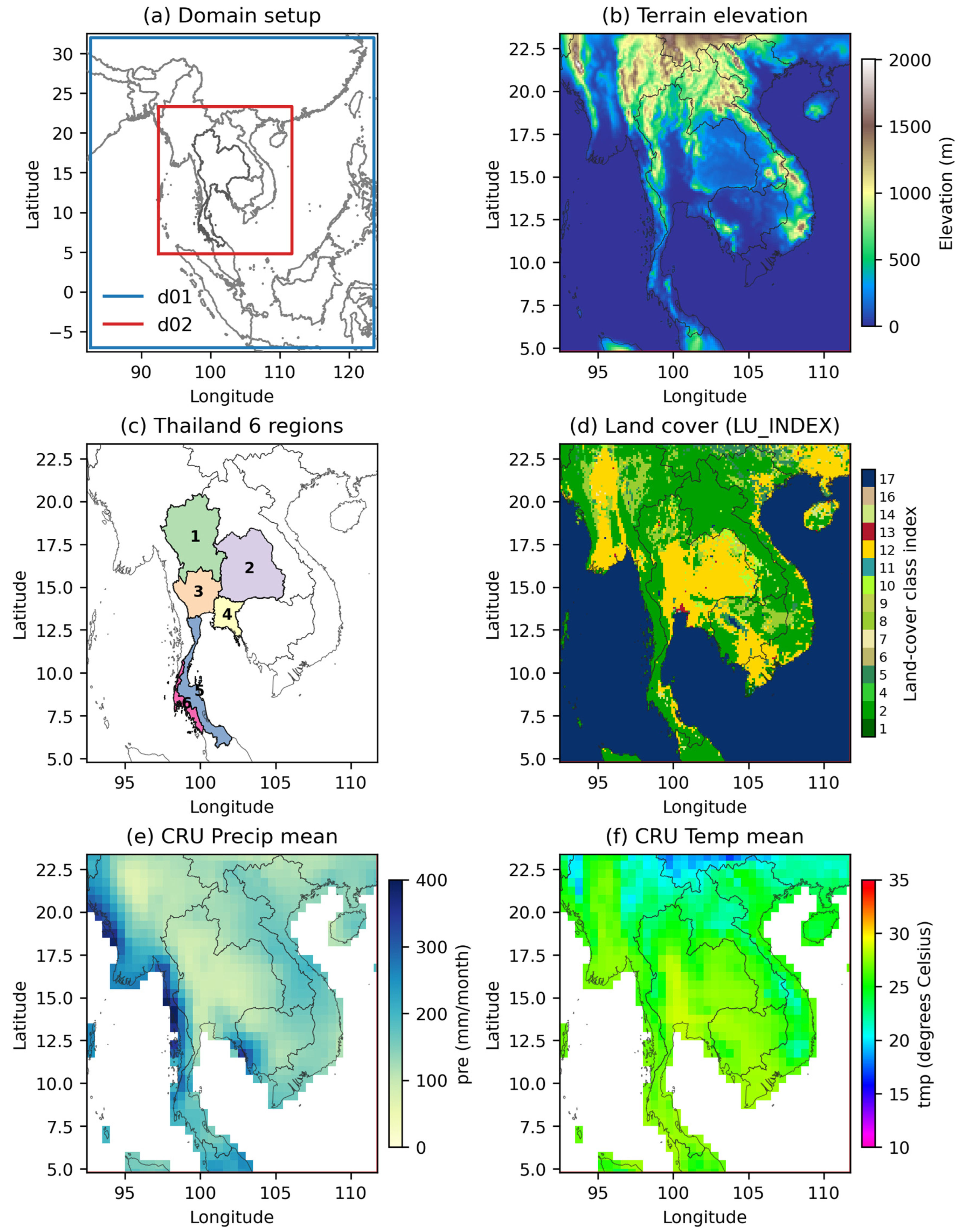
Disclaimer/Publisher’s Note: The statements, opinions and data contained in all publications are solely those of the individual author(s) and contributor(s) and not of MDPI and/or the editor(s). MDPI and/or the editor(s) disclaim responsibility for any injury to people or property resulting from any ideas, methods, instructions or products referred to in the content.

Article Metrics

Citations

Article Access Statistics

Multiple requests from the same IP address are counted as one view.