Abstract
It is interesting to identify the reasons and the direction of the correlation between the input/output prices and the macro/micro parameters in animal production processes. In the present study, the time series of the monthly data between the years 2014 and 2019 were analyzed to examine the factors that affected the consumer price of carcass meat in Turkey. An attempt was made to identify the relationship between the consumer price of carcass meat and the prices of cattle fattening feed, the exchange rate of the dollar, producer price index (PPI), and the agricultural PPI, which were anticipated to affect the consumer price of carcass meat as determined by the Granger causality analysis. According to econometric analysis results, when there is a change in carcass producer price, cattle fattening feed and PPI in the short term, the consumer price of carcass meat is affected by this. The producer price of carcass and PPI variables are determined to be the cause of each other’s Granger. At the same time, the PPI variable and the consumer price of carcass meat and dollar rate variables were found to be the cause of each other’s Granger. If Turkey is to prevent the excessive fluctuations in the consumer- and producer-prices of carcass meat caused by macro variables, an effective price control mechanism should be put into practice. It seems that this change would be possible only by developing and implementing policies to lower the input prices and production costs.
1. Introduction
Red meat production in Turkey was approximately 1.1 million tons as of 2019. Of this production, 89.7% was beef, and 10.3% was mutton, goat meat, and water buffalo meat [1]. The percentage share of beef in the red meat consumption has increased over the years [2]. As the per capita consumption of beef in Turkey is responsive to the prices, the consumption decreases as the prices increase [3,4,5]. However, policies and market interventions intended to prevent the fluctuations in red meat prices from past to present have fallen short of eliminating the insatiability and the ambiguity in the prices [6].
Feed costs have the highest share of the costs incurred by businesses producing red meat, next only to the costs of cattle fattening materials [7,8]. Feed input is an important cost factor in beef cattle breeding and directly affects the unit costs of the producers [9]. Due to the external dependence on the supply of raw materials and additives used in feed production in Turkey, the feed prices are adversely affected by changes in foreign exchange rates in the short term [10]. At the same time, forecasting the price levels in the livestock industry is a rather complicated process, as there are multiple factors that affect the prices. For example, it has been stated that the food price index, oil price, global food index, and exchange rates of the dollar and euro significantly affect the producer prices of animal and agricultural products [11].
Identifying the reasons for and the direction of the correlation between the input/output prices and macro/micro parameters in the animal production processes is important. When the causality correlation between two variables is examined, the contribution of the delayed value of one variable to explain the current value of the other variable is explicated by the theory of causality [12]. In this context, causality analysis has become a widely used method of analysis in studies on animal husbandry [13,14,15].
Causality analysis is successfully used to explain the effects of feed prices on cattle prices [13], lamb prices on beef prices [14], feed raw materials on live cattle prices [15], producer price index on feed prices [16], beef prices on consumer price index [17], and the US Dollar on agricultural commodity prices [18].
The purpose of this study was to investigate the causality relationship between the consumer price of red meat and the factors that affect this price between 2014 and 2019, with econometric methods. Red meat is focused upon throughout the article; used synonymously with veal and beef.
2. Materials and Methods
2.1. The Dataset
Time series of the monthly data for the period 2014–2019 were analyzed to identify the factors influencing the consumer price of red meat, i.e., the dependent variable in the study [19]. Producer price of carcass meat sourced by General Directory of Meat and Milk Board [19], price of fattening feed [20], the exchange rate of dollar [21], PPI, and agricultural PPI [22], were used as independent variables in the dataset of the study. As only the monthly data were used, a 72-period dataset was created in each time series. The effect of independent variables on consumer price of red meat was analyzed within the framework of the model below:
- Consumer Price of Red Meat = yt
- β1 = Price of Fattening Feed (TL/ton) (PFF),
- β2 = Producer Price of Carcass Meat (PFCM),
- β3 = Exchange Rate of Dollar (ERD),
- β4 = PPI,
- β5 = Agricultural PPI (APPI),
- yt = β0 + β1 (PFF) + β2 (PFCM) + β3 (ERD) + β4 PPIi + β5 APPI
The Eviews 8 program was used in the analysis of the time series [23], For an econometric model to proceed significantly, it is very important that the series in the model remain stationary. The time series in the variables were investigated to achieve this [24]. If the stationarity of a series is not examined, unrealistic relationship structures will be revealed, and the problem of spurious regression will occur [25]. The stationarity of the variables was put to Augmented Dickey–Fuller (ADF) and Phillips and Perron (PP) unit root tests when investigating the relationship between the variables. After the series became stable, the relationships in the econometric model were addressed separately for long and short terms. Engle–Granger and Johanson Cointegration tests were used to demonstrate the long-term relationship. To begin with, Vector Autoregression (VAR) estimation was performed and a suitable lag count was specified based on the VAR. Considering the lag counts, a long-term co-integration relationship was identified in the analysis. As there was a long-term co-integration, it was understood that the Vector Error Correction Model (VECM) should be used instead of the VAR model. In accordance with this result, the VECM model was used to analyze the relationship between the variables. The causality and the direction of the relationships between the variables in this model were examined together. The Granger causality test was applied to achieve this, and the test results were recorded.
2.2. Unit Root Tests
PP and ADF unit root tests were used to investigate the stationarity of the series. The PP test can be used to prevent autocorrelation as a nonparametric method if the error terms show an altering variance. ADF test, on the other hand, eliminates the problem of autocorrelation completely. In both the root tests, a lag length that would generate white noise for the error terms of all series is identified. Multiple information criteria are used to determine the lag length in these tests. The most used among these criteria are Akaike (ACI), Schwarts (SIC), Final Prediction Error (FPE), Hannan–Quinn (HQ), and (LR) [26,27].
2.3. ADF Unit Root Test
The different hypotheses in the ADF test yielded different results. A null hypothesis states that the series are not stationary, whereas an opposite hypothesis states that they are stationary. It is possible to show the ADF test with a constant with the following Equation (1) [28]:
To reject the null hypothesis in the ADF test, the variable Y should be accepted as stationary at its original level. Otherwise, it will be revealed that it is not stationary. As seen from the equation, differences between the series should be calculated so that the series that are not stationary at their original levels shall remain stationary. If the series becomes stationary when the difference is calculated for the first time, such series are called First-Degree Integrated series. If the series does not become stationary during the first time, the process continues until it becomes stationary. The t-statistics calculated with Equation (1) is compared with MacKinnon’s critical values to decide if a series is critical. Thus an absolute value is taken and if the MacKinnon’s critical value is smaller than the absolute value at different significance levels, the series is not considered stationary; if it is larger than the absolute value at different significance levels, then the series is concluded as stationary [29,30].
2.4. PP Unit Root Test
PP test is a sort of a supplementary test for the ADF unit root test. The equations in the ADF test assume that the error terms are statistically formed by a constant and independent variance. If we compare the assumptions of the PP unit root test and the ADF test, it turns out that PP root test has more flexible assumptions. As in the ADF root test, the null hypothesis in a PP unit root test also concludes that it is a unit root, i.e., the series is not stationary, but the opposite hypothesis concludes that the series is stationary. The PP stationarity test is shown in Equations (2) and (3) [26]:
In Equations (2) and (3), T represents the number of observations, εt represents the distribution of the error terms, yt represents the tested series, and α, β, and t represent the trend variables. In the PP test, it is assumed that there is a weak dependence between them and error terms are heterogeneously distributed. In order to eliminate the autocorrelation in the PP test, the method of correction with the Newey–West estimator is used for the results of the regression.
2.5. Co-Integration Tests
The existence of long-term relationships between the variables has been determined with multiple and various co-integration tests in the literature. Some of these tests are the Eagle–Granger Two-Step Cointegration test, Johansen’s Maximum Likelihood Vector Autoregressive method, Engle–Yoo’s Three-Step Cointegration test, Johansen–Juselius Cointegration test, and the Saikkonen Cointegration test. In the present study, the balanced relationships between the price of carcass meat, price of fattening feed (TL/Ton), the exchange rate of dollar, PPI, and the agricultural PPI were investigated with the Eagle–Granger and Johansen co-integration tests, which work well with long-term relationships.
2.6. Results of Johansen Cointegration Test
When the time series in this analysis were examined, it was seen that these series were equally stationary, and thus the co-integration test was applied. Firstly, VAR was estimated without any constraint in the values of these variables, and a suitable lag count was identified. The VAR method, first implemented by Sims, allows for dynamic and wide-ranging analysis of the relationships among the variables in the model [31]. It is an improved version of the Granger causality test; it attempts to estimate the dynamic relationships between the endogenous variables without any restriction [32]. VAR analysis is based on a simultaneous equations model. In VAR analysis, it is explained by the lagged values of both the endogenous and the other variables. The equations used in a standard bivariant VAR analysis are as given below (Equations (4) and (5)):
The constant term indicated by ai0 in Equations (4) and (5) is the parameter of the lag of the variable j in equation ai, uit is the error term and p is the lag count [29]. The lag lengths of the variables in VAR analysis should be the same so that the symmetry of the model is maintained and the EKK estimator becomes active. Akaike (ACI), Schwarts (SIC), Hannan–Quinn (HQ), (LR) and Final Prediction Error (FPE) information criteria were used to determine the suitable lag length in VAR models [26,27]. In order to determine the existence of a long-term relationship between the series identified as cointegrated with the Engle–Granger co-integration test and the count of cointegrated vectors, the multi-cointegration test developed by Johansen and Juselius was used. For this, the trace and maximum eigenvalue test statistics were used. The critical values used in both the tests were generated by Johansen and Juselius. In order to accomplish this, the optimal lag length was determined before switching to the model to be estimated.
2.7. VECM and Granger Causality Test
The VECM is estimated to investigate the short-term dynamics of two or more series acting in unison in the long run. The co-integration equations obtained as a result of the estimation were tested with the Granger causality test, and the direction of causality/relationships between the variables was revealed.
The VECM is represented by the following Equations (6) and (7):
If there is a co-integration relationship between the variables in yt, the rank is (∏) = r < k. There are two kxr matrices, as α and β confirm the equation of ∏ = αβ. Matrix α is composed of coefficients of the adjustment velocity, and matrix β is composed of the co-integration vectors [33].
VECM was estimated because a co-integration relationship was identified between the variables. Equations showing the co-integration relationships obtained from this estimate were tested later by the Granger causality test.
The Granger causality test was used to investigate the causality between the variables. The significance of the lag values of the independent variable in the equations was tested using the Granger causality test [34].
3. Findings
The results of the unit root test applied to the variables are presented in Table 1.

Table 1.
The results of the unit root test applied to the variables.
The findings obtained from the results of the ADF and the PP unit root tests are as follows: the consumer price of red meat, price of fattening feed, producer price of carcass meat, the exchange rate of dollar, PPI, and the agricultural PPI were not stationary in some forms, but when their first differences were taken, the series became stationary at 1% significance level, i.e., with a constant and without a trend, without a constant and trend, with a constant and trend.
As seen in the Collegrom chart (Consumer Price of Carcass Meat, Price of Fattening Feed (TL/Ton), Producer Price of Carcass Meat, Exchange Rate of Dollar, PPI and Agricultural PPI) autocorrelation, partial autocorrelation and their significance are shown in detail in Figure 1.
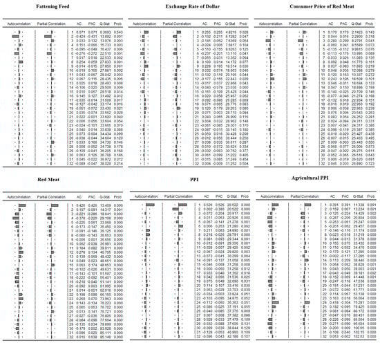
Figure 1.
Correlogram Charts of the Data Related to the Consumer Price of Carcass Meat, Price of Fattening Feed (TL/Ton), Producer Price of Carcass Meat, Exchange Rate of Dollar, PPI and Agricultural PPI, First Degree Differences of Which Were Taken.
The selection of appropriate lag lengths for the VAR model is presented in Table 2.
Table 2.
Selection of suitable lag lengths for the VAR model.
In determining the lag length of the model, the suitable count of lags was found to be 1 according to the FPE, AIC, SC, and the HQ information criteria. While the AIC criterion is based on the minimization of the mean square error and is rather a value considered in forward-looking forecasts, the HQ criterion is a value that is used in determining the consistent level of a lag. Therefore, as seen in the above table, the lag length 1 was stable according to the analysis results.
The results of the Johansen co-integration test are presented in Table 3.
Table 3.
Results of the Johansen Cointegration Test.
After identifying the suitable lag count for the Johansen co-integration test, the existence of a long-term relationship between the variables was tested. By using the predicted VAR equation, the existence of the Johansen co-integration was investigated (Table 3). When the co-integration test statistics were examined, it was seen that there were five co-integration vectors where the hypothesis H0 was rejected. The trace and the eigenvalue tests indicated that these five variables acted in unison in the long term.
The results of the Granger causality test for the consumer price of red meat are presented in Table 4.
Table 4.
Results of the Granger causality test for the consumer price of red meat.
As seen from the results of the causality tests in Table 4, the consumer price of red meat was affected in the short term by the changes in the producer price of carcass meat, price of fattening feed, and PPI between 2014 and 2019. In other words, the consumer price of the red meat was influenced by the producer price of carcass meat, the price of fattening feed, and the PPI variables.
The Granger causality test findings for the producer price of carcass meat are presented in Table 5.
Table 5.
The results of the Granger causality test for the producer price of carcass meat.
According to the results of the causality test shown in Table 5 the producer price of carcass meat was affected in the short term by the changes in the price of fattening feed between 2014 and 2019. In other words, the producer price of carcass meat was the Granger causality of the price of fattening feed.
The results of the Granger causality test for the exchange rates of dollars are presented in Table 6.
Table 6.
The results of the Granger causality test for the exchange rate of dollar.
According to the results of the causality test shown in Table 6 the exchange rates of dollar were affected in the short term by the changes in the producer price of carcass meat between 2014 and 2019. In other words, the exchange rate of the dollar was the Granger causality of the producer price of carcass meat and PPI variables.
The results of the Granger causality test for the PPI are presented in Table 7.
Table 7.
The results of the Granger causality test for PPI.
According to the results of the causality test, as summarized in Table 7, PPI was affected in the short term by the changes in the consumer price of the red meat and the exchange rate of dollar between 2014 and 2019. In other words, the PPI is the Granger causality of the consumer price of red meat and the exchange rate of dollar variables.
The results of the Granger causality test for the agricultural PPI are presented in Table 8.
Table 8.
The results of the Granger causality test for Agricultural PPI.
According to the results of the causality test in Table 8, the agricultural PPI in dollars was affected in the short term by the changes in the consumer price of the red meat between 2014 and 2019. In other words, the agricultural PPI is the Granger causality of the consumer price of red meat.
4. Discussion
The relationships between the consumer price of the red meat and the producer price of carcass meat, price of cattle fattening feed, the exchange rate of dollar, PPI, and the agricultural PPI, which affected the price of the red meat, were examined by way of Granger causality analysis.
The results of the analysis revealed that the consumer price of the red meat was affected by short-term changes in the producer price of carcass meat, price of the fattening feed, and the PPI. The interactions between the producer price of carcass meat and the consumer price of veal were as expected. It was reported that only between 47.05% and 66.32% of the retail price paid by the consumers for the veal was received by the producers [35]. The price of fattening feed seriously affects the production cost of veal. Although the production and the consumption of fattening feed have quadrupled in Turkey in the last 15 years, the production of the feed raw materials has not increased proportionally [10]. When the changing exchange rates are added to meet the supply deficit by way of imports, the price of fattening feed becomes very high [21]. Previous studies have also revealed that the macro variable, PPI, directly affected the prices of feed [16].
The present study revealed that the changes in the price of fattening feed reflected on the producer price of carcass meat in the short term. In line with the policies pursued to decrease the producers’ costs, the tax rate in the fattening feed was reduced in Turkey as of 1 January 2016 [36]. However, when Granger causality analysis was applied to check the short-term effect of the said tax cut, it was observed that the cut did not affect the prices of feed, meat, or milk [37]. Therefore, it is very important to use the right policy tool to intervene in the interaction between the producer price and the price of fattening feed. It was predicted in the present study that the prices of both the red meat and the fattening feed will increase in the forthcoming years [2]. When an assessment is made on local beef production, productivity levels per animal are compared especially to European Union countries, Turkey is behind in the beef carcass yield 1.5 times [38].
In a study covering the periods between 2010/1 and 2015/2 in the USA, the relationship between corn, soybean and wheat and live cattle prices was found to be bidirectional. With this bilateral relationship, it has been stated that both grain products, live cattle prices are the cause of granger, and live cattle prices are the causes of grain products [15].
In a study in which the effect of the dollar index on global commodity prices in the period between January 1999 and February 2015 with an asymmetric causality test, no long-term relationship between the US dollar and agricultural commodity indices was found. In the short term, the depreciation of the US dollar leads to the rise in agricultural commodity prices, while the appreciation of the US dollar causes the prices of all commodities in the scope of the analysis to decrease [18].
Chen et al. examined Australia, Canada, Chile, New Zealand and South Africa in their studies, and stated that exchange rates can be used to predict future food prices [39]. Harri et al. used the VAR model covering the monthly period between 2000–2008 in the USA and found that the same result does not apply to wheat, while there is an integration relationship between corn, cotton, soybean and crude oil prices and exchange rates [40]. Gilbert states that world GDP growth, monetary expansion, oil price and dollar exchange rate have a causal effect on agricultural food commodity prices [41].
5. Conclusions
The present study found that a change in the producer price of the carcass meat is affected by the exchange rate of dollar and the PPI in the short term. Depending on the macro variables, it is possible to prevent only the excessive fluctuations in the producer price of carcass meat with an effective price control mechanism. Consequent to the constantly increasing input costs such as those of feed, labor, energy, and fuel, the producers would need a market created by the product councils and institutions like the Meat and Milk Institution, which would, in turn, be supported by long-term production and consumption policies.
In order to reduce the input costs, the prices of inputs such as fuel and electric power used in the livestock industry should be reduced. As the feed costs have an important share in the carcass meat production costs in Turkey, local production of feed raw materials such as import-dependent soybean and corn should be encouraged. Some recent global events, such as the Covid-19 outbreak, have proven again the need for the countries to attain independence in the production of staple foodstuff.
Knowing the direction of the relationship between the price of the product and the prices of input goods in animal husbandry would lead to adopting effective courses of action and forming efficacious policies to support the industry, beginning from the sub-industries. Ensuring a better understanding of the relationships between the input and output prices in the veal market may particularly lead Turkey to better plan the future production of veal to decrease the import dependencies and become self-sufficient in the area.
Author Contributions
Conceptualization, B.M., M.S.A., and M.A.T.; methodology, M.A.T. and M.B.Ç.; validation, M.B.Ç., A.C.A. and M.A.T.; investigation, B.M., M.S.A., M.B.Ç., A.C.A. and M.A.T.; resources, A.C.A.; data curation, M.B.Ç. and A.C.A.; writing—original draft preparation, B.M.; writing—review and editing, B.M. and M.S.A.; supervision, B.M.; project administration, M.A.T. and M.S.A. All authors have read and agreed to the published version of the manuscript.
Funding
This research received no external funding.
Conflicts of Interest
The authors declare no conflict of interest.
References
- MFAL 2019 Livestock Data, Ministry of Agriculture and Forestry of Turkey. Available online: https://www.tarimorman.gov.tr/sgb/Belgeler/SagMenuVeriler/HAYGEM.pdf (accessed on 15 March 2020).
- Cicek, H.; Dogan, I. Developments in Live Cattle and Beef Import and the Analysis of Producer Prices with Trend Models in Turkey. Kocatepe Vet. J. 2018, 11, 1–10. [Google Scholar]
- Erdogdu, H.; Cicek, H. Modeling beef consumption in Turkey: the ARDL/bounds test approach. Turk. J. Vet. Anim. Sci. 2017, 41, 255–264. [Google Scholar] [CrossRef]
- Bölük, G.; Karaman, S. Market power and price asymmetry in farm-retail transmission in the Turkish meat market. New Medit. 2017, 16, 2–11. [Google Scholar]
- Ayyıldız, M.; Çiçek, A. Analysis of red meat prices with Garch method: The case of Turkey. Turk. J. Agric. Food Sci. Technol. 2018, 6, 1775–1780. [Google Scholar]
- Arikan, M.S.; Cevrimli, M.B.; Akin, A.C.; Tekindal, M.A. Determining the change in retail prices of veal in Turkey by GARCH method between 2014–2017. Kafkas Univ. Vet. Fac. Mag. 2019, 25, 499–505. [Google Scholar]
- Celik, S.; Sariozkan, S. Economic Analysis of Cattle Fattening Enterprises in the Center of Kirsehir Province. Harran Univ. J. Fac. Vet. Med. 2017, 6, 38–45. [Google Scholar]
- Aydin, E.; Sakarya, E. Economic analysis of intensive cattle fattening enterprises in the provinces of Kars and Erzurum. Kafkas Univ. Vet. Fac. Mag. 2012, 18, 997–1005. [Google Scholar]
- Arikan, M.S.; Gokhan, E.E. The effect of preliminary body weight of the Limousin cattle on the economic fattening performance. Eurasian J. Vet. Sci. 2018, 34, 228–232. [Google Scholar]
- CBRT. The Key Structural Factors Underlying High Red Meat Prices in Turkey: High Animal Feed Prices. The Central Bank of the Republic of Turkey. 2018. Available online: http://tcmbblog.org/wps/wcm/connect/blog/en/main+menu/analyses/red+meat+prices+in+turkey (accessed on 12 November 2018).
- Bayramoglu, A.T.; Yurtkur, A.K. International Factors on Food and Agricultural Price Determinations in Turkey. Anadolu Univ. J. Soc. Sci. 2015, 15, 63–73. [Google Scholar]
- Engeloglu, O.; Meral, I.G.; Genc, K. Literature review on casualty implementations for Turkey. Soc. Sci. Res. J. 2015, 4, 142–154. [Google Scholar]
- Arslan, S. The effect of fuel prices on the prices of small cattle and cattle. Int. Manag. Econ. Bus. Mag. 2017, 1, 284–291. [Google Scholar]
- Yalcinkaya, H. Investigation on the compatibility of Ankara meat stock exchange with the efficient market hypothesis. J. Bus. Res. Türk 2017, 9, 495–509. [Google Scholar]
- Fiszeder, P.; Orzeszko, W. Nonlinear Granger causality between grains and livestock. Agric. Econ. Czech 2018, 64, 328–336. [Google Scholar]
- Yalcinkaya, H. Factors affecting concentrate feed prices. TÜBAV J. Sci. 2016, 9, 13–22. [Google Scholar]
- Akin, A.C.; Cevrimli, M.B.; Arikan, M.S.; Tekindal, M.A. Determination of the causal relationship between beef prices and the consumer price index in Turkey. Turk. J. Vet. Anim. Sci. 2019, 43, 353–358. [Google Scholar] [CrossRef]
- Buberkoku, O. The Impact of the US Dollar’s Movements on Commodity Prices. Ege Acad. Rev. 2017, 17, 323–336. [Google Scholar]
- GDMMBs: General Directory of Meat and Milk Board. Weekly Meat Price Bulletin. Available online: https://www.esk.gov.tr/ (accessed on 9 February 2018).
- TFIA. Turkey Feed Statistics. Turkish Feed Industrialists Association. 2018. Available online: http://www.yem.org.tr/Birligimiz/isistikler (accessed on 11 November 2018).
- CBRT. Indicative Exchange Rates, Central Bank of the Republic of Turkish. 2018. Available online: https://www.tcmb.gov.tr/wps/wcm/connect/EN/TCMB+EN/Main+Menu/Statistics/Exchange+Rates/Indicative+Exchange+Rates (accessed on 23 May 2018).
- TSI, Agricultural Price Statistics, Turkish Statistical Institute. Available online: https://biruni.tuik.gov.tr/medas/?kn=110&locale=en (accessed on 15 November 2018).
- EViews, version 8; IHC Markit: London, UK, 2016.
- Goktas, O. Theoretical and Applied Time Series Analysis; Besir Publishing House: İstanbul, Turkey, 2005. [Google Scholar]
- Granger, C.W.J.; Newbold, P. Spurious in econometrics. J. Econ. 1974, 2, 111–120. [Google Scholar] [CrossRef]
- Johansen, S. Likelihood-Based Inference in Cointegrated Vector Autoregressive Models; Oxford University Press: Oxford, UK, 1995. [Google Scholar]
- Enders, W. Applied Econometric Time Series; Jonh Wiley & Sons. Inc.: New York, NY, USA, 1995. [Google Scholar]
- Asteriou, D.; Hall, S.G. Applied Econometrics: A Modern Approach, revised edition; Palgrave Macmillan: Hampshire, UK, 2007; Volume 46, pp. 117–155. [Google Scholar]
- Tari, R. Econometrics, Revised and Extended, 3rd ed.; Kocaeli University Publications: Kocaeli, Turkey, 2005; p. 263. [Google Scholar]
- Yilmaz, O.; Akinci, M. The relationship between economic growth and current account balance: The Case of Turkey. Ataturk Univ. J. Soc. Sci. Inst. 2011, 15, 363–377. [Google Scholar]
- Ozer, M.; Coskun, I.O. Sustainability of Turkish current account deficit in the post crisis period. Nibes Trans. 2011, 5, 67–82. [Google Scholar]
- Sims, C. Macroeconomics and reality. Econometrica 1980, 48, 1–49. [Google Scholar] [CrossRef]
- Johansen, S. Estimation and hypothesis testing of co-integration vectors in gaussian vector autoregressive models. Econometrica 1991, 59, 1551–1580. [Google Scholar] [CrossRef]
- Granger, C.W. Investigating causal relations by econometric models and cross-spectral methods. Econom. J. Econom. Soc. 1969, 37, 424–438. [Google Scholar] [CrossRef]
- Aral, Y.; Cevrimli, M.B.; Akdogan, N.; Aydin, E.; Arikan, M.S.; Akin, A.C.; Ozen, D. Investigation of intermediary margins in the marketing of beef and lamb meat in Ankara province, Turkey. Kafkas Univ. Vet. Fac. J. 2016, 22, 685–691. [Google Scholar]
- TOG. Decision on the Determination of the Value Added Tax Rates, Special Consumption Tax Rates and Amounts and Tobacco Fund Amounts to be Applied to Some Goods. Turkish Official Gazette, 2016 1 January; 29580. [Google Scholar]
- Yalcinkaya, H.; Aktas, M.A. Impact of vat rates of feed on meat and milk prices. J. Marmara Univ. Soc. Sci. Inst. Recomm. 2019, 14, 38–60. [Google Scholar]
- Sakarya, E.; Gökdai, A.; Şahin, T.S. Livestock policies and read meat sector: Republic period and ensuing years. J. Istanb. Vet. Sci. 2019, 3, 64–74. [Google Scholar] [CrossRef]
- Chen, Y.; Rogoff, K.; Rossi, B. Can exchange rates forecast commodity prices? Q. J. Econ. 2010, 125, 1145–1194. [Google Scholar] [CrossRef]
- Harri, A.; Nalley, L.; Hudson, D. The relationship between oil, exchange rates, and commodity prices. J. Agric. Appl. Econ. 2009, 41, 501–510. [Google Scholar] [CrossRef]
- Gilbert, C.L. How to understand high food prices. J. Agric. Econ. 2010, 61, 398–425. [Google Scholar] [CrossRef]

© 2020 by the authors. Licensee MDPI, Basel, Switzerland. This article is an open access article distributed under the terms and conditions of the Creative Commons Attribution (CC BY) license (http://creativecommons.org/licenses/by/4.0/).