Mexico’s Forest Diversity: Common Tree Species and Proposed Forest-Vegetation Provinces

Abstract

We report a relatively rare study of a national forest inventory in a megadiverse country with the systematic collection of herbarium specimens. The taxonomic identification of 22,659 herbarium collections from 6942 sites of Mexico’s national forest inventory resulted in 1464 native tree species (approximately half of Mexico’s estimated total), in 470 genera and 117 plant families. We compared visual tree-species identifications in the field by hired crews, with much more rigorous identification of submitted (mostly sterile) herbarium specimens by experienced taxonomists and specialists at the National Herbarium: for 40% of the 22,659 collections, the identification of species names from the field was confirmed, for 32% it was corrected at the herbarium, and 27% had been sent without any identification. The most commonly collected plant families were Fagaceae (oak family, 21.7% of all collections), Fabaceae (legumes, 17.7%), and Pinaceae (pine family, 13.3%). The most commonly collected tree species in six major forest-vegetation types were Pinus leiophylla in “coniferous forest”, Quercus magnoliifolia in “highland broadleaf forest”, Liquidambar styraciflua in “mountainous cloud forest”, Bursera simaruba in “lowland evergreen forest”, Lysiloma divaricatum in “lowland dry forest”, and Parkinsonia microphylla in “xerophilous scrub”. We overlapped the six major forest-vegetation types with Mexico’s 15 mainland floristic provinces, as circumscribed by Rzedowski. This resulted in 75 so-called forest-vegetation provinces, of which 35 had at least 20 collection sites. The similarity of species composition among these 35 forest-vegetation provinces was only 17–34% with the Jaccard community index, and 15–42% with the Morisita-Horn community index. The number of physically undetected species was estimated statistically for the 35 forest-vegetation provinces, which indicates that there are forest-vegetation provinces, where the number of species could be up to 8.8-fold higher than those detected in the present work. Finally, we suggest a method to distribute sites optimally among the country in future forest inventories, such as to minimize the average area represented by the sites in each forest-vegetation province.

1. Introduction

The number of all Mexican native plant species has been estimated to be roughly around 22,000–23,000 [1,2]. Many plant families have not been revised in recent decades, and new species are frequently published, or species names are changed. Descriptions for a proportion of Mexico’s plant species, including trees, can be found in the literature, such as published volumes of the Flora Mesoamericana and regional flora projects. A complete, integral Flora of Mexico project, however, does not yet exist.

The number of native tree species in Mexico depends on how one defines the term, which varies among the following publications. The classical work has been Standley’s Trees and shrubs of Mexico from 1920–26 [3], with about 5700 species (page 1643 in [3]). Standley, however, included many smaller shrub species, as well as exotic species, but more important is that after about a century, the work’s taxonomy is outdated. In 1998, Villaseñor and Ibarra-Manríquez [4] estimated 3639 tree species for Mexico, with 42% being endemic, but did not provide a species list. A recent reference has been Pennington and Sarukhán’s manual from 2005 [5] (first edition in 1968), with the description of 190 tropical tree species from Mexico, which however represent less than 10% of all Mexican tree species. Ricker and Hernández in 2010 [6] defined trees or tree-like plants more rigorously as “perennial, self-supporting plants with an height of at least 5 m at maturity in situ (without ascending leaves or inflorescences), and with one or several erect stems with a diameter of at least 10 cm”; tree species or tree-like species “contain individuals with tree characteristics at least somewhere in its geographic range.” In four articles, Ricker and collaborators from 2010 to 2020 provided an updated but still partial taxonomic list under that definition, with 1250 species in 26 families, of which 43% are endemic in Mexico [6,7,8,9]. Finally, Téllez and collaborators in 2020 [10] analyzed the diversity and distribution of Mexico’s native tree species, for which they compiled an (available) list of 2885 species, of which 44% are endemic.

Collections of herbarium specimens in most countries have rarely been taken homogeneously over the area of a whole country [11]. This makes it difficult to determine which tree species are the most common ones, and to compare floristically different regions. Furthermore, forest inventories are designed to measure forest cover homogeneously for a whole country. In a megadiverse country such as Mexico, however, species identifications are challenging for field teams that measure trees for a forest inventory. In 2009, the National Herbarium of Mexico (MEXU), which forms part of the Biology Institute of Mexico’s national university (UNAM), started a collaboration with Mexico’s national forest agency CONAFOR (Comisión Nacional Forestal), to carry out the taxonomic identifications of trees. After a pilot study, field teams were asked to send at least one specimen of each distinct tree species per 1600 m² study site to the herbarium. The collaboration provided a unique opportunity to analyze and report here tree species occurrences for the whole of Mexico.

Forest inventories have been carried out in Mexico in varying forms and coverage since the 1960s [12]. The current design and methods of Mexico’s national forest inventory, however, started in 2004 (

Table 1. Summary about national forest inventories in Mexico.

Spanish Name of Forest Inventory	Result
Primer Inventario Nacional Forestal 1961–1985 (24 years)	Maps, volume tables, reports for some states
Inventario Nacional Forestal de Gran Visión 1991	Maps with forest vegetation, first report about the situation of forests on a national scale
Inventario Nacional Forestal Periódico 1992–1994	Maps with forest vegetation, dasometric statistics
Inventario Nacional Forestal 2000	Maps with vegetation types and geographic data, created via remote sensing [15]
Inventario Nacional Forestal y de Suelos 2004–2009	Per-tree measurements and collections for analysis on 21,743 sites, id est, subdivided areas of 1600 m2 [13]
Inventario Nacional Forestal y de Suelos 2009–2014	Per-tree measurements and collections for analysis on 22,409 sites, id est, subdivided areas of 1600 m2 [14]
Inventario Nacional Forestal y de Suelos 2015–2020	Per-tree measurements and collections for analysis on 10,686 sites, id est, subdivided areas of 1600 m2

); for the most recent report of results, see [13,14]. In addition, there have been state-level forest inventories. The most recent reports for each state in Mexico can be found at https://old-snigf.cnf.gob.mx/inventario-estatales/ (accessed on 17 September 2022).

There are three widely recognized systems for the classification of Mexico’s vegetation types: Miranda and Hernández’s classification from 1963 [16], Rzedowski’s from 1978 [17], and the one in the maps about land use and vegetation from Mexico’s National Institute of Statistics and Geography (abbreviated INEGI in Spanish), being updated every few years (https://www.inegi.org.mx/temas/usosuelo/, accessed on 17 September 2022). These systems combine, as classification criteria, plant physiognomy, together with climate, elevation, dominance by species, and in the case of the INEGI, status after disturbance and current land use. Except for the disturbance status, the categories can be translated to some extent from one system into another. Concerning floristic origin and composition, there has only been one classification of “floristic provinces” for the whole of Mexico by Rzedowski (chapter 6 in [17]), with the map by Rzedowski and Reyna-Trujillo from 1990 [18].

Despite the challenge of identifying over three-quarters of the collections without flowers or fruits, we report here the results of 9247 collections from the year 2013, 8217 collections from 2014, 3819 collections from 2015, 707 pilot-study collections from 2009 to 2011, and 669 collections from 2016. Our specific objectives were:

• to identify as many collections as possible, given mostly sterile collections, and to discuss identifying species in the field versus by specialists in the national herbarium;
• to define and present (in maps) major forest-vegetation types for Mexico, and subdivide them into “forest-vegetation provinces”;
• to present and analyze the frequency of the collected species;
• to compare species-composition similarity among forest-vegetation provinces;
• to statistically estimate the total species richness of forest-vegetation provinces that include the number of physically undetected species, and determine forest-vegetation provinces with high potential to collect previously uncollected species.

2. Materials and Methods

2.1. Study Area and Field Work

Mexico’s national forest inventory (Inventario Nacional Forestal y de Suelos) covers all of Mexico’s continental area. There is no universally accepted quantification of the land area of Mexico, with scientifically reported methods and assumptions for comparisons: The total land surface with islands, reported by Mexico’s National Commission for the Knowledge and Use of Biodiversity (abbreviated CONABIO in Spanish) in November 2019, after taking into account coastal changes, is 1,954,658 km². We will refer to that value, which is 0.49% smaller than the 1,964,375 km² previously reported by Mexico’s National Institute of Statistics and Geography (INEGI), but 0.55% larger than the 1,943,950 km² stated by the World Bank; the latter defines a country’s total area to exclude area under inland water bodies.

To implement forest inventories, Mexico’s national forest agency CONAFOR (Comisión Nacional Forestal) goes through a bidding process to contract companies or institutions that carry out the field work. Three companies were involved for the present study: AMAREF (Zapopan, Jalisco, Mexico), DIAAPROY (Mexico City, Mexico), and INYDES (Texcoco, State of Mexico, Mexico). The companies hire people that form three-person field crews, and generally include biologists, foresters, or related professionals. Occasionally, there are also local field assistants. The 22,659 collections were collected by 278 distinct people. For the botanical collections, we provided two manuals [19,20]. The goal was to make one collection of each distinct tree species per 1600 m² plot (a collection consists ideally of several “duplicate” herbarium specimens from the same tree). That goal was not always met, either because field crews did not recognize a given tree as a distinct species, or because of difficulties to access the flowers or fruits of large trees. The dried herbarium specimens were sent or delivered to the Biology Institute, where they were deep-frozen $(-70 °\mathrm{C})$ for three days to kill insects, before being processed further.

2.2. Species Identifications

Once the specimens shipped to the national herbarium (MEXU) were unpacked, plant families were identified and specimens separated accordingly by (coauthors) Esteban M. Martínez and Clara H. Ramos. Even though 54 specialists participated in the taxonomic identifications (see acknowledgments), 90% of the 22,659 collections were identified at the species-level by the five coauthors Clara H. Ramos, Mauricio A. Mora, Jorge Calónico, Esteban M. Martínez, and Leandro J. Ramos. This resulted in high consistency for identifying many of the species that appeared repeatedly.

Our first version of the database with identifications contained 33,025 herbarium collections, of which 23,920 had been identified at the species level, 573 tentatively at the species level, 4719 only at the genus level, 26 tentatively at the genus level, and 3787 only at the family level. The exclusion of collections that were not identified at the species level (or only tentatively), and that did not represent trees, tree-like plants, or at least large shrubs, resulted in the 22,659 collections of the present study.

2.3. Elaboration of Maps

Maps were created with the software ArcGIS 10.8.1. To relate the thematic layers with the collection sites, the ArcGIS’s Intersect tool was used (https://desktop.arcgis.com/en/arcmap/latest/tools/analysis-toolbox/how-intersect-analysis-works.htm, accessed on 17 September 2022). Apart from the geographic coordinates of the collection sites, the following input layers were used:

• Land use and vegetation map, series VI (base year 2014, presented in 2017), of Mexico’s National Institute of Statistics and Geography (INEGI) from https://www.inegi.org.mx/app/biblioteca/ficha.html?upc=889463598459 (accessed on 17 September 2022);
• Floristic provinces, defined by Rzedowski and Reyna-Trujillo in 1990 [18], from http://www.conabio.gob.mx/informacion/gis/ (Regionalización—Bióticas—Divisiones florísticas), accessed on 17 September 2022;
• Political divisions of Mexico’s states from https://www.inegi.org.mx/temas/mg/ (accessed on 17 September 2022).

2.4. Confidence Intervals for Proportions and Statistical Analyses

Statistical analyses were carried out with Mathematica (www.wolfram.com/mathematica/), and—where indicated—with R-functions. For the most common tree species, the number (frequency) of sites with a presence of the species in a given major forest-vegetation type $(n_0)$ was determined as a proportion of the number of sites $(n)$ with a presence of the species in all six major forest-vegetation types together. If collections are homogeneous in space, in a way to be representative for the area of interest, then the estimated probability of the presence of the species in the given forest-vegetation type is $n_0/n.$ The corresponding lower and upper limits of the Clopper–Pearson confidence limits for $n_0/n$ are ([21] and pages 25–26 in [22]):

$$P_L=\frac{n_0}{n_0+\left(n-n_0+1\right)\cdot F_L}, P_U=\frac{\left(n_0+1\right)\cdot F_U}{\left(n-n_0\right)+\left(n_0+1\right)\cdot F_U},$$

(1)

where $F_L$ is the value of the statistical F-distribution with $2\cdot \left(n-n_0+1\right)$ and $2\cdot n_0$ degrees of freedom, and significance level $\alpha$ (probability of a type I error: the risk of concluding that a difference exists, when there is no actual difference; typically $\alpha$ = 0.05). If $n_0=0$, then $P_L$ is 0. Furthermore, $F_U$ has $2\cdot \left(n_0+1\right)$ and $2\cdot \left(n-n_0\right)$ degrees of freedom, with significance level $\alpha .$ Note that the intervals resulting with (1) are asymmetric.

To calculate confidence intervals for multiples comparisons, the significance level $\alpha$ was adjusted for the number of groups (k) that were compared. As a conservative and easy way, we employed the Bonferroni method (or Bonferroni correction). For a family-wide error rate of $\alpha =0.05$, one adjusts ${\alpha }_{adj.}=\alpha /k$, so that in the case of six comparisons, ${\alpha }_{adj.}=0.0083$ (page 67 in [23] and page 239 in [24]).

The resulting confidence intervals can be compared pairwise: non-overlapping 95% confidence intervals imply that a significance test between two means would detect a significant difference below the 5% significance level (the wider the gap, the lower the probability that the two means could belong to the same statistical population). However, confidence intervals that overlap slightly do not imply necessarily that a significance test would not detect a significant difference [25]. The reason is that a standard significance test between two estimated means ${\widehat{M}}_1$ and ${\widehat{M}}_2,$ that follow a normal distribution, correspond to calculating if the interval $\left({\widehat{M}}_1-{\widehat{M}}_2\right)\pm 1.96\cdot \sqrt{{\widehat{SE}}_1^2+{\widehat{SE}}_2^2}$ includes zero. Comparing two confidence intervals corresponds to observe if ${\widehat{M}}_1\pm 1.96\cdot {\widehat{SE}}_1$ and ${\widehat{M}}_2\pm 1.96\cdot {\widehat{SE}}_2$ overlap. The overlap method is less powerful to detect different means, because $1.96\cdot {\widehat{SE}}_1+1.96\cdot {\widehat{SE}}_2\ge 1.96\cdot \sqrt{{\widehat{SE}}_1^2+{\widehat{SE}}_2^2}$ converts to ${\widehat{SE}}_1\cdot {\widehat{SE}}_2\ge 0,$ which is always true. Confidence intervals in a graph, however, are a very compact and intuitive way to present differences among means.

2.5. Jaccard and Morisita-Horn Similarity Indices among Provinces for Each Major Forest-Vegetation Types

The original Jaccard index [26] calculates similarity based on the presence or absence of a number of species in two communities. The Morisita-Horn index [27,28,29] in addition takes the relative abundance into account. Both indices were originally developed for pairwise comparisons. The corresponding community indices for more than two comparisons simultaneously were derived by Jost (Equation (8) in [30]) for the Jaccard index, and by Chao and collaborators (Equation (13) in [29]) for the Morisita-Horn index. The formulas employed here are from pages 78 and 84 in [31], with adjusted notation, and were implemented in a Mathematica notebook. The similarity indices are always between 0 (no species shared) and 1 (all species shared, in the case of the Morisita-Horn index with equal relative abundance).

Both pairwise and community indices were calculated among floristic provinces within a given forest-vegetation type. Since the Jaccard and Morisita-Horn similarity indices for communities (>2 provinces) are the more general cases, from which the pairwise indices can be derived, they are presented first:

$$J_N=\frac{\overline{S}/S-1/N}{1-1/N},$$

(2)

$$M{H}_N=1-\frac{{\displaystyle \sum _{i=1}^S{\displaystyle \sum _{k>m}^N{\left(p_{im}-p_{ik}\right)}^2}}}{\left(N-1\right)\cdot {\displaystyle \sum _{i=1}^S{\displaystyle \sum _{k=1}^N{p}_{ik}^2}}},$$

(3)

where

• $J_N:$ the Jaccard similarity index for species richness among N floristic provinces (as $U_{0N}$ on page 84 in [31]);
• $M{H}_N:$ the Morisita-Horn similarity index for relative species incidence among N floristic provinces (as $C_{2N}$ on page 84 in [31]); and
• i, m, k: counting indices, where i refers to the counting number of species, m to the compared first floristic province, and k to the compared second floristic province;
• N: the number of floristic provinces in the analyzed forest-vegetation type;
• p: relative abundance of the species in the province (or probability to encounter it); it is calculated as the number of incidences (or detections) of a given species in a given province, as a proportion of the number of incidences of all species in the floristic province; in the present study, the number of incidences corresponds to the number of collection sites where the species was found;
• $S:$ the total number of species in all N floristic provinces;
• $\overline{S}$: the average number of species per floristic province: $\overline{S}=\left({\displaystyle {\sum }_{k=1}^N{S}_k}\right)/N,$ where $S_k$ is the number of species in province k.

The Jaccard similarity index $J_N$ among N entities (here provinces) simplifies to the widely known Jaccard index $J_2$ for two samples, when one substitutes in (2) $S=S_1+S_2-S_{12}$ and $\overline{S}=\left(S_1+S_2\right)/2,$ where $S_1$ is the number of positive encounters in the first sample, $S_2$ the number of positive encounters in the second sample, and $S_{12}$ the number of shared encounters. Equation (2) then becomes:

$$J_2=\frac{S_{12}}{S_1+S_2-S_{12}}.$$

(4)

Similarly, for the Morista–Horn index, Equation (3) reduces to

$$M{H}_2=1-\frac{{\displaystyle {\sum }_{i=1}^S{\left(p_{i1}-p_{i2}\right)}^2}}{{\displaystyle {\sum }_{i=1}^S\left(p_{i1}^2+p_{i2}^2\right)}}.$$

(5)

In contrast to the Jaccard index, the Morisita-Horn index is not an indicator of pure species richness, but an indicator that takes into account how often a species has been encountered in a floristic province. This requires homogeneously distributed sampling (page 153 in [32]), which can be assumed here with sufficient approximation, given standardized collection sites that are to some extent evenly distributed. The Morisita-type index is sensitive to the relative proportion of the most abundant species (page 365 in [33]).

Chao and collaborators in 2006 [33] developed abundance-based similarity indices that take the number of physically undetected species statistically into account (see Section 2.6). Their objective was to reduce the bias of comparisons that omit estimates of the varying number of undetected species. The formulas are given on pages 69 and 85–86 in [31]. We add the corresponding estimates of the community indices, as calculated with the R-function SimilarityMult from the SpadeR package (with specifications “incidence_freq”, “q = 2”, and “nboot = 1”). We do not report bootstrap confidence intervals, as included in [31], because we think that more research and documentation is needed on that aspect. For example, what variation is being accounted for with the bootstrap confidence intervals? In Chao’s approach, pairs of species abundances between two assemblages are resampled (page 6 in the supplementary material of [33]). This implies that the abundances are always fixed for given species. Consequently, however, the resulting confidence intervals do not account for the variation (error) in estimating abundances.

2.6. Species Richness Estimation for Forest-Vegetation Provinces

The methods of estimating the number of physically undetected (or unseen) species, that are used here, go back to Burnham and Overton in 1978 [34] and Chao in 1984 [35], with many subsequent publications. The idea is that the number of detected rare species, such as the number of singletons (species detected once) and doubletons (species detected twice) is mathematically related to the number of species that can still be detected. With the lower-bound Chao1-estimator (page 69 in [31]), the number of undetected species will go toward zero, if the observed number of singletons is small relative to the observed number of doubletons.

Total species richness (detected plus undetected) of forest-vegetation provinces was estimated with three estimators, employing the R-function ChaoSpecies from the SpadeR library (with specifications “incidence_freq” and “k = 10”, where “k” stands for $\kappa$). The formulas for the three estimators are the following:

$${\widehat{S}}_{iChao2}={\widehat{S}}_{Chao2}+\frac{T-3}{4\cdot T}\cdot \frac{Q_3}{Q_4}\cdot Max\left[Q_1-\frac{T-3}{2\cdot \left(T-1\right)}\cdot \frac{Q_2\cdot Q_3}{Q_4},0\right],$$

(6)

$$\begin{array}{c}{\widehat{S}}_{ICE1}=D_{freq}+\frac{D_{infreq}}{{\widehat{C}}_{infreq}}+\frac{Q_1}{{\widehat{C}}_{infreq}}\cdot \\ Max\left[\left({\widehat{S}}_{ICE}-D_{freq}\right)\cdot \frac{T_{infreq}}{T_{infreq}-1}\cdot \frac{{\displaystyle \sum _{i=1}^{\kappa }\left[i\cdot \left(i-1\right)\cdot Q_i\right]}}{{\displaystyle \sum _{i=1}^{\kappa }\left[i\cdot Q_i\right]}\cdot \left({\displaystyle \sum _{i=1}^{\kappa }\left[i\cdot Q_i\right]}-1\right)}-1,0\right],\end{array}$$

(7)

$${\widehat{S}}_{jack2}=D+\frac{2\cdot T-3}{T}\cdot Q_1-\frac{{\left(T-2\right)}^2}{T\cdot \left(T-1\right)}\cdot Q_2,$$

(8)

with

$${\widehat{S}}_{Chao2}=\{\begin{array}{l}D+\frac{\left(T-1\right)\cdot Q_1^2}{2\cdot T\cdot Q_2} \mathrm{for} Q_2>0,\\ D+\frac{\left(T-1\right)\cdot Q_1\cdot \left(Q_1-1\right)}{2\cdot T} \mathrm{for} Q_2=0,\end{array}$$

$$\begin{array}{cc}{\widehat{S}}_{ICE}=\hfill & D_{freq}+\frac{D_{infreq}}{{\widehat{C}}_{infreq}}+\frac{Q_1}{{\widehat{C}}_{infreq}}\cdot \hfill \\ & Max\left[\frac{D_{infreq}}{{\widehat{C}}_{infreq}}\cdot \frac{T_{infreq}}{T_{infreq}-1}\cdot \frac{{\displaystyle \sum _{i=1}^{\kappa }\left[i\cdot \left(i-1\right)\cdot Q_i\right]}}{{\displaystyle \sum _{i=1}^{\kappa }\left[i\cdot Q_i\right]}\cdot \left({\displaystyle \sum _{i=1}^{\kappa }\left[i\cdot Q_i\right]}-1\right)}-1,0\right],\hfill \end{array}$$

where

• $\widehat{S}:$ the estimated number of detected plus undetected species by a specified estimator;
• ${\widehat{S}}_{iChao2}:$ the iChao2 estimator of the number of species ([36] and pages 22 and 70–71 in [31]); by using not only singletons (species detected in exactly one sampling unit) and doubletons (species detected in exactly two sampling unit), but also tripletons and quadrupletons, it represents an improved lower bound, compared with the Chao2 estimator;
• ${\widehat{S}}_{ICE1}:$ the ICE-1 is the Incidence-based Coverage Estimator for highly heterogeneous cases [37]: the non-parametric ICE separates frequent and infrequent species into two groups, and only the infrequent group is used to estimate the number of undetected species (pages 21–23 and 71 in [31]);
• ${\widehat{S}}_{jack2}:$ the second-order jackknife estimator for incidence data [34] uses singletons and doubletons to estimate the number of undetected species (pages 16 and 71 in [31]); the first-order and second-order jackknife estimators are more reliable than higher-order jackknife estimators [38];
• ${\widehat{S}}_{Chao2}:$ the Chao2 estimator of the number of species [39];
• ${\widehat{S}}_{ICE}:$ the Incidence-based Coverage Estimator [37]; and
• ${\widehat{C}}_{infreq}:$ estimated sample coverage for the infrequent species group, defined as $1-{\displaystyle {\sum }_{i=1}^{T_{infreq}}\left[i\cdot Q_i\right]}/{\displaystyle {\sum }_{i=1}^T\left[i\cdot Q_i\right]};$ see page 69 in [31];
• $D:$ number of distinct species detected in the sample;
• $i:$ counting index;
• $\kappa :$ cut-off point between infrequent and frequent species in the two ICEs, which here was chosen to be 10, meaning that species found on more than 10 sites are considered frequent;
• $Max\left[term,0\right]:$ if $term>0,$ then the result is term, otherwise the result is 0;
• $Q_i:$ number of species that are detected in exactly i sampling units (i = 1, 2, …, T);
• $T:$ total number of sites;
• $T_{infreq}:$ number of sampling units that includes at least one infrequent species.

3. Results

3.1. Classification of Mexico’s Forests into Major Forest-Vegetation Types

Forest classification was based on series VI of the INEGI’s land use and vegetation map (base year 2014, presented in 2017). The map includes 183 land cover categories, distinguishing vegetation types and their disturbance levels (former forests with secondary tree, shrubby, or herbaceous vegetation) and other land uses, such as agriculture and urban areas. We grouped 107 categories into seven major forest-vegetation types, whereas 76 categories remained as “Other surfaces” (for details see Supplementary Material S1). The main characteristics of the INEGIs vegetation types within the 183 categories are described in [40].

Table 2. Major forest-vegetation types of Mexico and their areas (ordered from high to low elevations, and vicinity).

Forest-Vegetation Type	Area (km2)	Relative Area
(1) Coniferous forest (bosque de coníferas)	166,764	8.53%
(2) Highland broadleaf forest (bosque latifoliado de montaña)	157,064	8.04%
(3) Mountainous cloud forest (bosque mesófilo de montaña)	18,023	0.92%
(4) Lowland evergreen forest (selva perennifolia)	98,470	5.04%
(5) Lowland dry forest (selva caducifolia)	203,888	10.43%
(6) Xerophilous scrub (matorral xerófilo)	536,713	27.46%
Subtotal:	1,180,922	60.42%
(7) Mangrove and wetland forests (manglares y bosques de humedales)	10,135	0.52%
Other surfaces:	763,601	39.07%
Total:	1,954,658	100%

shows the chosen names of the seven major forest-vegetation types in English and Spanish, together with their absolute and relative areas in Mexico (ordered from high to low elevations and vicinity). Mangrove and wetland forests are separated in the table, because they are not subdivided into forest-vegetation provinces in the next section. The seven major forest-vegetation types are shown in the map in Figure 1, together with the 6942 collection sites of the present study.

3.2. Classification of Mexico’s Forests Area into Forest-Vegetation Provinces

We were interested in a subclassification that reflects evolutionary formed species associations in currently existing forests. A total of 17 floristic provinces have been proposed for Mexico by Jerzy Rzedowski in 1978 [17], and were updated in a map by Rzedowski and Reyna-Trujillo in 1990 [18]. Of these, 15 are shown in the map of Figure 2, together with the names of the Mexican political states, in which they lie. Two additional floristic provinces that are restricted to relatively small islands are not considered here, because they were not included in the forest inventory: the Guadalupe-island province and the Revillagigedo-islands province. Overlapping the delimitations of the first six major forest-vegetation types of Table 2 (Figure 1) with the delimitations of Rzedowski’s 15 floristic provinces (Figure 2) results in 75 subunits that we define as “forest-vegetation provinces”. Mangroves and wetland forests were not included; being dominated by the presence of water in any region, the concept of floristic provinces does not apply comparably.

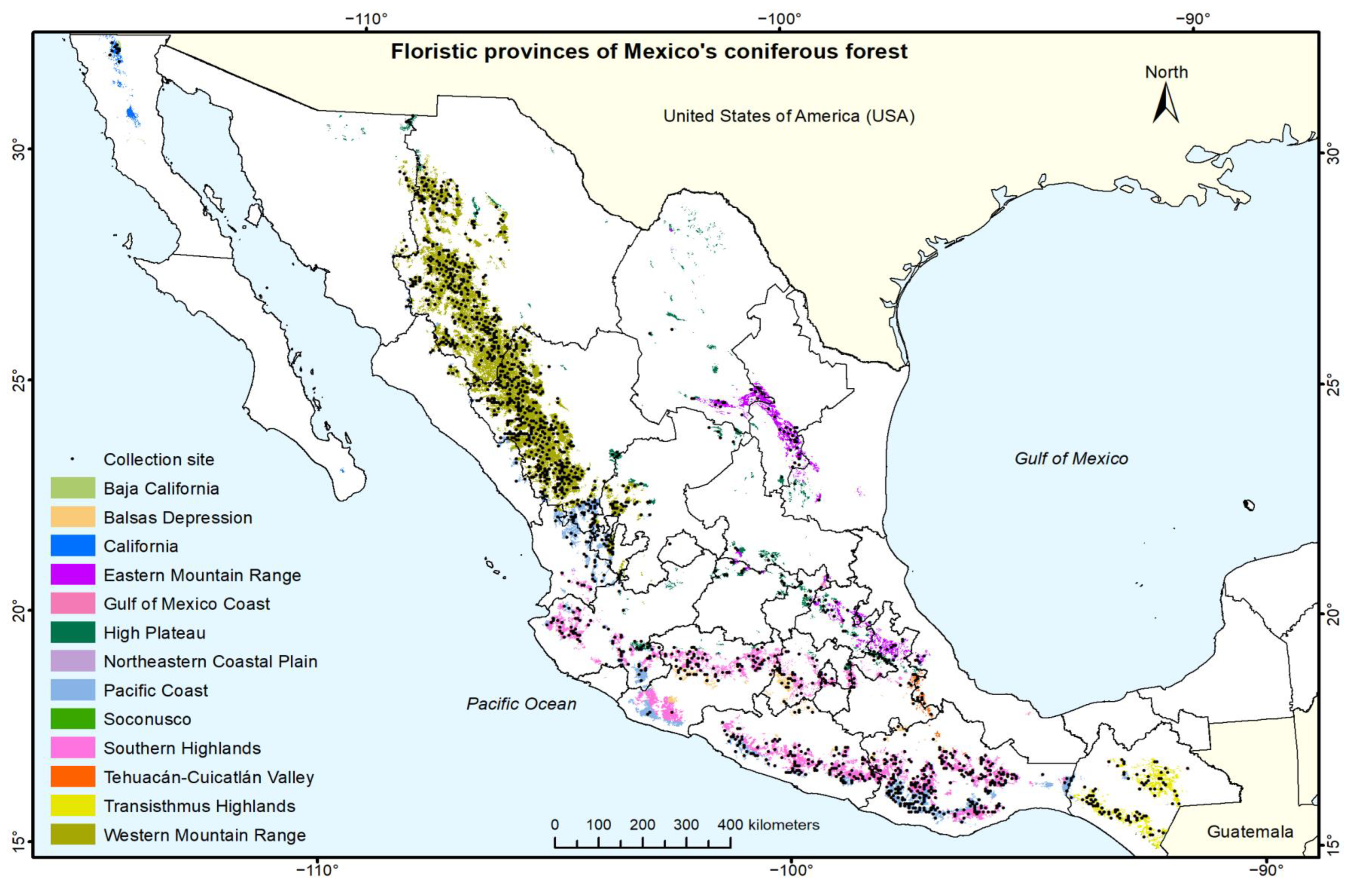
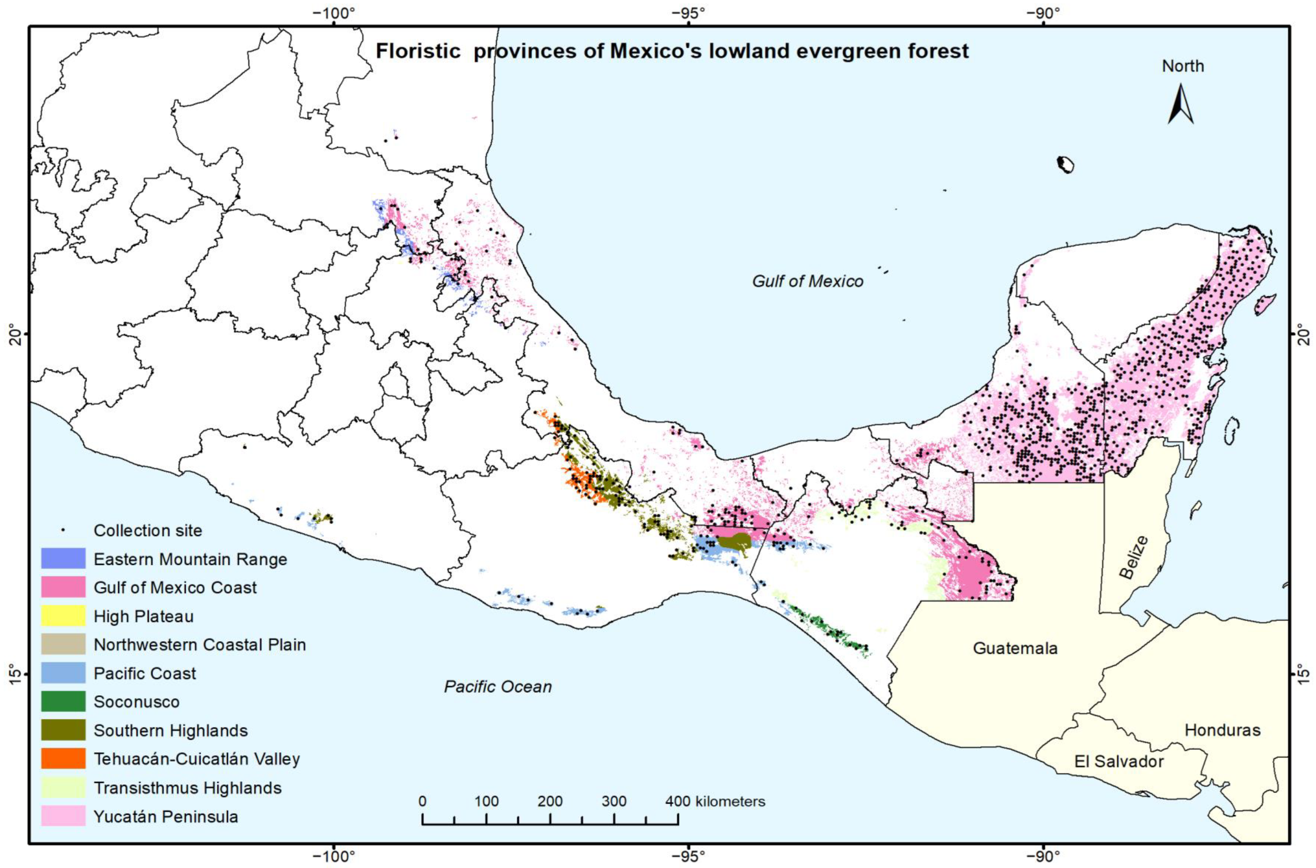
The 75 forest-vegetation provinces are listed in Supplementary Material S2 in English and Spanish, together with their absolute and relative areas. The sum of all forest-vegetation provinces is 1,180,922 km², which corresponds to 60.42% of Mexico’s land area (Table 2). The distributions throughout Mexico of forest-vegetation provinces, in each of the six major forest-vegetation types, are presented in the maps in Figure 3, Figure 4, Figure 5, Figure 6, Figure 7 and Figure 8. In addition, Figure 9 shows a map of the distribution of mangrove and wetland forests.

3.3. Results of Species Identifications and Collection Effort

We identified 22,659 herbarium specimen collections from 6942 sites, corresponding to 1464 tree or tree-like species in 470 genera and 117 plant families. Remarkably, the species identifications were possible even though approximately 77% of the herbarium collections were sterile, and only 23% had flowers or fruits. Information per species is provided in Supplementary Material S3, including information about the number of herbarium collections (each with “duplicate” specimens from the same tree), geographical locations and elevations, major forest-vegetation types, and floristic provinces.

Compared to the number of native tree species, there were few exotic ones: 28 species were collected (see Supplementary Material S4). Particularly well-known are Citrus species (oranges etc.) from Southeast Asia, Coffea arabica (coffee) from northeast Africa, Eucalyptus species from Australia, and Mangifera indica (mango) from tropical Asia.

Table 3. Collection effort in Mexico for this study.

Major Forest-Vegetation Type	Area in Mexico (km2)	Relative Area of Mexico	Corresponding Number of Herbarium Collections	Inverse Collection Density (km2/Collection)	Collections on Sites with Secondary Vegetation
Coniferous forest	166,763	8.5%	7089	23.5	37%
Highland broadleaf forest	157,064	8.0%	4917	31.9	40%
Mountainous cloud forest	18,024	0.9%	867	20.8	58%
Lowland evergreen forest	98,470	5.0%	2694	36.6	67%
Lowland dry forest	203,888	10.4%	4192	48.6	73%
Xerophilous scrub	536,713	27.5%	598	897.5	12%
Mangrove and wetland forest	10,135	0.5%	384	26.4	7%
Other surfaces	763,506	39.1%	1924	396.8	-
Mexico	1,954,658	100%	22,659	86.2	-

shows the collection effort in the major forest-vegetation types. The second-last column gives the area for the corresponding major forest-vegetation type in Mexico (second column), divided by the number of herbarium collections in our study (third column), or in other words, the average area represented by each collection in the forest-vegetation type. Xerophilous scrub stands out with 897.5 km², but is not directly comparable, because of large areas in Mexico without sufficiently large plants that should be considered trees or tree-like plants. Mountainous cloud forest has the highest collection effort (20.8 km² per collection), but also has the smallest area (18,024 km²). That is a 2.3-times higher collection effort than for lowland dry forest (48.6 km² per collection). Overall, the collection efforts among “true” forest types (id est, excluding xerophilous scrub) is not drastically different, although the collection density with 21 to 49 km² per collection is obviously low, due to the country’s extension.

The diversity of large trees particularly in primary lowland evergreen forests remains probably underrepresented here. For mountainous cloud forest, lowland evergreen forest, and lowland dry forest, over half of the collection sites are classified by the INEGI as secondary vegetation (last column in Table 3). Furthermore, 90% of all collections were from trees with a height in the range of 3.3 to 16.7 m, with a median of 7.2 m.

3.4. Most Frequently Detected Species

The intended strategy of the herbarium collections was to register only distinct tree species in each 1600 m² plot, so that the number of collections of a given species equals the number of plots where it was found. Counting each species once per plot is also necessary for the subsequent analyses.

For that reason, 938 collections that repeated some species on some site were excluded for the numerical analyses of frequencies and distributions. After the exclusion, there were 21,721 collections, representing 1464 species in 470 genera and 117 families on 6942 sites.

Table 4. Ten most frequently collected families, genera, and species, respectively, in all of Mexico (in all columns 100% = 21,721 collections).

Family Collections	Number of Genera	Number of Species	Genus Collections	Number of Species	Species Collections
Fagaceae (21.7%)	1	105	Quercus (21.7%)	105	Pinus leiophylla (1.78%)
Fabaceae (17.7%)	68	261	Pinus (12.9%)	32	Quercus magnoliifolia (1.67%)
Pinaceae (13.3%)	3	39	Lysiloma (3.8%)	8	Juniperus deppeana (1.65%)
Malvaceae (4.5%)	22	51	Acacia (3.5%)	33	Acacia pennatula (1.58%)
Ericaceae (4.2%)	9	22	Arbutus (3.3%)	6	Guazuma ulmifolia (1.45%)
Burseraceae (3.4%)	2	64	Bursera (3.2%)	60	Pinus cembroides (1.43%)
Cupressaceae (3.1%)	3	18	Juniperus (2.9%)	14	Pinus oocarpa (1.39%)
Anacardiaceae (2.6%)	14	37	Guazuma (1.5%)	1	Lysiloma divaricatum (1.32%)
Euphorbiaceae (1.4%)	21	55	Ipomoea (1.2%)	5	Arbutus xalapensis (1.31%)
Convolvulaceae (1.2%)	1	5	Cordia (1.0%)	17	Lysiloma acapulcense (1.21%)

shows the ten most frequently collected families, genera, and species. Remarkable is the extensive presence of oaks, with 21.1% of the 21,721 collections representing the genus Quercus, and 105 detected species. Furthermore, Pinus leiophylla was the most frequently collected species (386 collections, each on a different site).

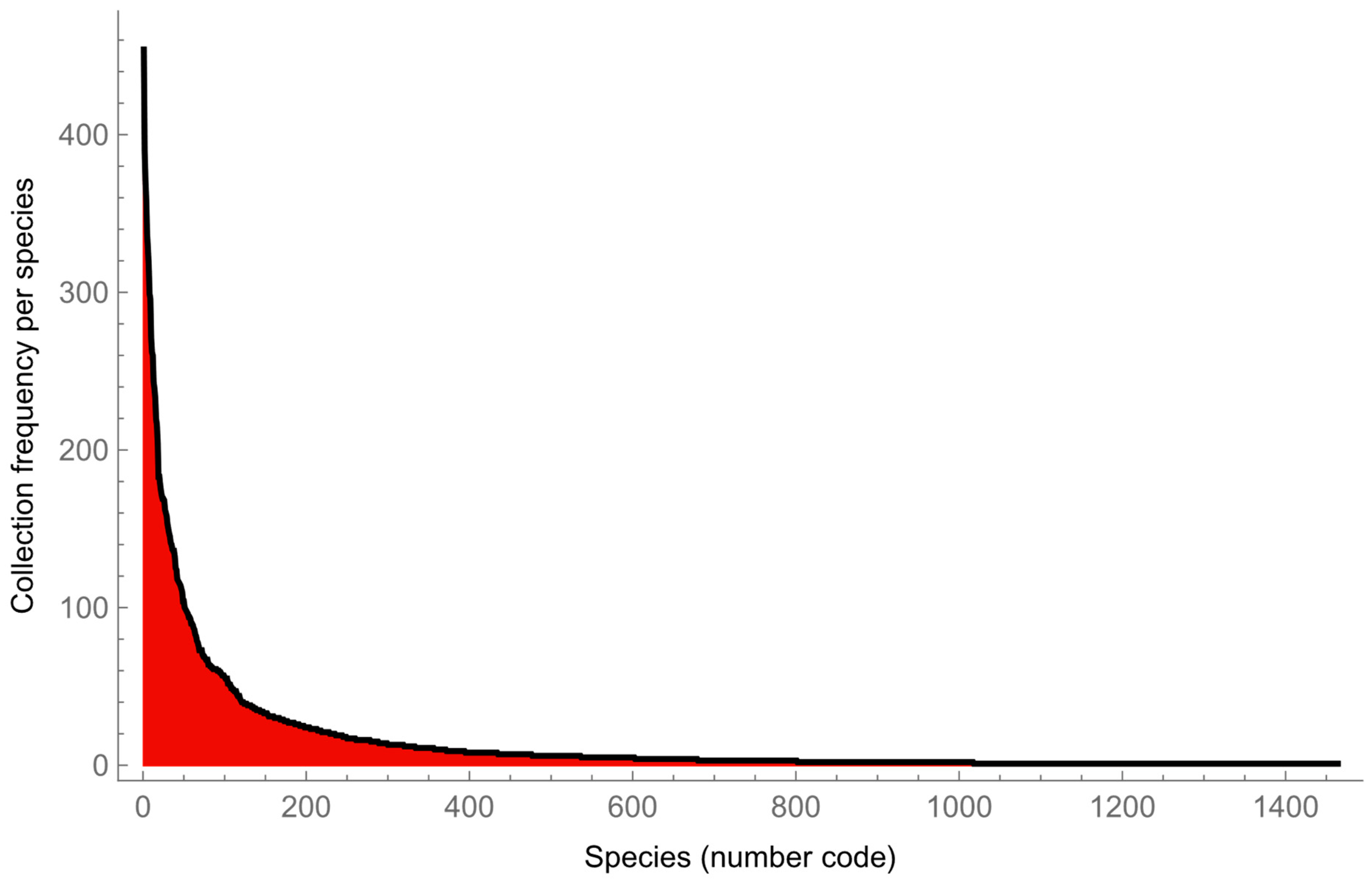
Figure 10 shows a graph of the number of collections per species for all 1464 species, in order of decreasing collection frequency. The initial peak (“species 1”) represents the 386 collections of Pinus leiophylla, whereas on the right, there are 452 species with a single collection. The distribution shows the general pattern that in diverse forest regions or countries only a few species are found abundantly.

Turning to the most frequent species in each of the six major forest-vegetation types, the following six species resulted:

• Pinus leiophylla (Pinaceae) and Juniperus deppeana (Cupressaceae) were most frequently found in coniferous forest, id est, they had the highest share of sites;
• Quercus magnoliifolia (Fagaceae) and Acacia pennatula (Fabaceae) in highland broadleaf forest;
• Liquidambar styraciflua (Altingiaceae) and Pinus pseudostrobus (Pinaceae) in mountainous cloud forest;
• Bursera simaruba (Burseraceae) and Manilkara zapota (Sapotaceae) in lowland evergreen forest;
• Lysiloma divaricatum (Fabaceae) and Guazuma ulmifolia (Malvaceae) in lowland dry forest; and
• Parkinsonia microphylla and Prosopis laevigata (both Fabaceae) in xerophilous scrub.

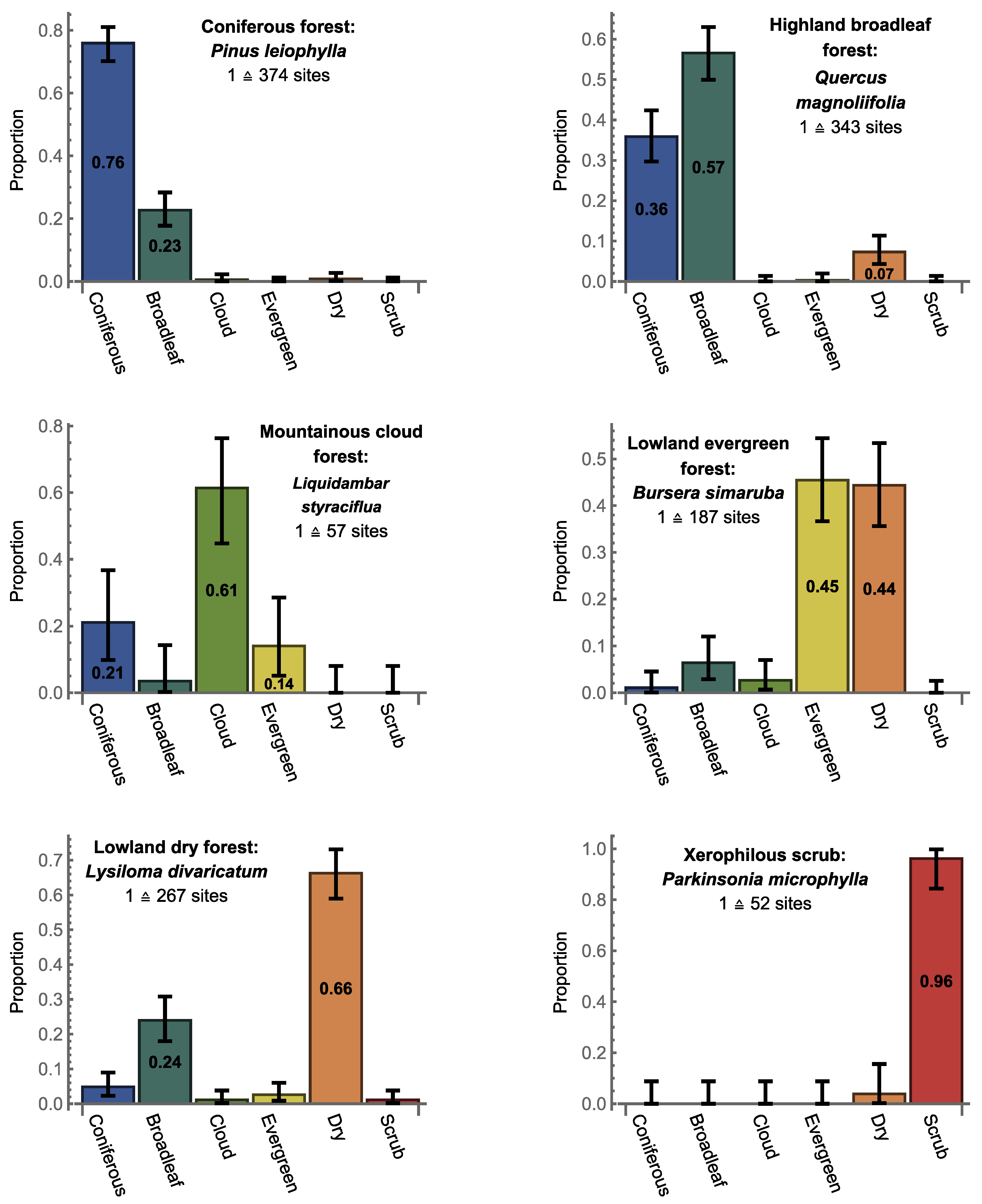
Figure 11 shows for each of the most frequent species the proportion of sites among the six major forest-vegetation types, where it was found. For example, Pinus leiophylla was found on 374 of the 6942 study sites in all of Mexico, and a proportion of 0.76 (284 sites) was found in coniferous forest, more sites than for any other species in coniferous forest. Bursera simaruba is a remarkable habitat generalist, which was almost as often collected in lowland dry forest as in lowland evergreen forest. Nevertheless, in lowland dry forest, Lysiloma divaricatum was found on even more sites. Figure 11 also shows 95% confidence intervals according to Equation (1), adjusted for simultaneous comparisons (six comparisons in each graph). If the intervals do not overlap, the differences of the bar height can be considered significantly different at a probability level that is lower than 5%. However, if the intervals overlap slightly, a significance test might still detect a difference of the corresponding proportions at the 5% level (see Section 2.4).

Concerning forest-vegetation provinces, the most commonly collected species are given in Supplementary Material S6, although only for the 35 forest-vegetation provinces with at least 20 collection sites (the number of 20 is arbitrary but reasonable to assure a minimum representation of species).

3.5. Differences among Species Compositions among Forest-Vegetation Provinces

The seven major forest-vegetation types in Table 2 can be seen as major divisions according to environmental niches and forest physiognomy (physical appearance). Our proposal to distinguish 75 forest-vegetation provinces subdivides them further according to floristic characteristics (Supplementary Material S5). For our proposal to be valid, we need to show that forest-vegetation provinces are floristically distinct. Whereas the number of sites is sufficiently large to compare species frequencies with confidence intervals for a low number of classes (Figure 11), such an approach is not useful for analyzing similarities (or differences) among the 75 forest-vegetation provinces. Instead, we calculate similarity indices pairwise, as well as community (similarity) indices, for all provinces per forest-vegetation type together.

Table 5. Similarity indices among forest-vegetation provinces (FVPs) for each major forest-vegetation type.

	Coniferous Forest	Highland Broadleaf Forest	Mountainous Cloud Forest	Lowland Evergreen Forest	Lowland Dry Forest	Xerophilous Scrub
Total number of FVPs	13	13	12	10	15	12
FVPs ≥ 20 sites	7	7	4	6	7	4
Total number of species in FVPs ≥ 20 sites	490	531	292	601	612	113
Number of species per FVP ≥ 20 sites: range	57–306	40–239	66–133	29–285	42–347	27–49
Pairwise Jaccard index: mean (range)	0.316 (0.147–0.616)	0.310 (0.152–0.639)	0.337 (0.275–0.442)	0.251 (0.069–0.522)	0.226 (0.054–0.569)	0.176 (0.077–0.295)
Jaccard community index (with unseen species)	0.328 (0.431)	0.332 (0.450)	0.336 (0.535)	0.275 (0.444)	0.239 (0.321)	0.171 (0.258)
Pairwise Morisita-Horn index: mean (range)	0.348 (0.106–0.742)	0.335 (0.106–0.730)	0.432 (0.280–0.534)	0.322 (0.055–0.797)	0.243 (0.007–0.757)	0.157 (0.063–0.285)
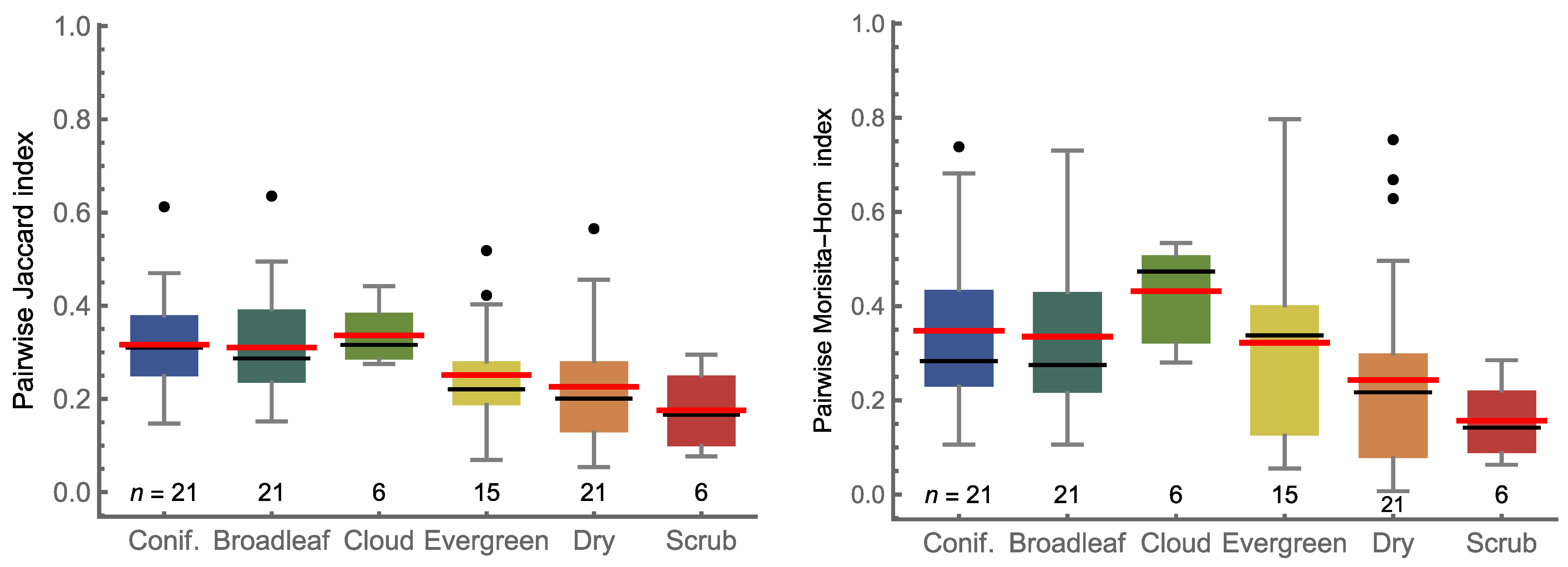
Morisita-Horn community index (with unseen species)	0.329 (0.348)	0.313 (0.332)	0.419 (0.468)	0.321 (0.354)	0.208 (0.215)	0.154 (0.165)

presents in the first row for each forest-vegetation type the total number of forest-vegetation provinces (FVPs), followed by those with at least 20 collection sites (to assure a minimum representation of species). The third row shows the number of detected species for the corresponding forest-vegetation provinces combined, and the fourth row the range of the number of species per forest-vegetation province. This is followed by the statistics of pairwise comparisons with the Jaccard index from Equation (4). In the first column, with seven forest-vegetation provinces, there are $\left(7^2-7\right)/2=21$ pairwise comparisons. The range of Jaccard similarity is from 0.147 to 0.616, with a mean of 0.316. The Jaccard community index from Equation (2) in the subsequent row is 0.328, and thus is similar but not equal to the mean of the pairwise comparisons. The community index that is bias-corrected for unseen species [33], under mathematical assumptions, is given in parentheses.

The community index does not imply that in this case 32.8% of the species are shared by all seven communities; that would be 161 of 490 species in the case of coniferous forest, but in reality, only 20 species are shared. If one looks at the formula of the Jaccard community index in Equation (2), the main component (apart from scaling) is $\overline{S}/S,$ the mean number of species per province divided by the total number of species in all provinces together. This can be interpreted probabilistically as the expected (mean) relative number of species in a province.

The last two lines in Table 5 provide the statistics of the pairwise similarities and community similarity with the Morisita-Horn index from Equations (3) and (5). Whereas the community Jaccard index takes into account all species in a forest-vegetation province without regard to their number of collections, the community Morisita-Horn index accounts for the relative abundance of each species. Nevertheless, here the Morisita-Horn indices (0.154 to 0.419) are not drastically different from the Jaccard indices (0.171 to 0.336); whether they are larger or smaller depends on the major forest-vegetation type.

Figure 12 shows box–whisker plots for the pairwise comparisons of the two indices. Importantly, the means of pairwise comparisons are far below 1. Furthermore, the ranges of the pairwise comparisons have a maximum of 0.639 in the case of the Jaccard index, and 0.797 in the case of the Morisita-Horn index, id est, no two forest-vegetation provinces within a forest-vegetation type share the same species composition. In conclusion, there is much dissimilarity among forest-vegetation provinces for a given forest-vegetation type. The conclusion does not change with community indices that are bias-corrected for unseen species, although the indices increase (Table 5). The six Jaccard community indices become on average 45% larger, and the Morisita-Horn indices on average 7%. The results support the classification into forest-vegetation provinces, in that there seem to be large differences in species composition among them.

There are other similarity indices that could be analyzed. For example, there is the “community regional-overlap index” (pages 84–85 in [31]). One can show that the community regional-overlap index is always larger than the Morisita-Horn community index. Ultimately, there is no “correct” diversity index to measure “true” diversity, and compare it among floristic provinces or other entities [41]. Rather, different indices have different properties, and have to be chosen accordingly.

3.6. Estimation of Undetected Species in Each Forest-Vegetation Province

The 75 forest-vegetation provinces are listed in Supplementary Material S2. Furthermore, Supplementary Material S5 provides in two columns the association between the 75 forest-vegetation provinces and the 1403 species detected in them (62 additional species were found outside). For the number of forest-vegetation provinces per species, the range is from 1 to 33, with a median of 2. For the number of species per forest-vegetation provinces, the range is from 1 to 347, with a median of 29. The forest-vegetation provinces with most species are “Lowland dry forest—Pacific Coast” (347 species), “Coniferous forest—Southern Highlands” (306), “Lowland evergreen forest—Gulf of Mexico Coast” (285), and “Highland broadleaf forest—Southern Highlands” (239). These are large forest-vegetation provinces, with 3.03%, 1.92%, 1.10%, and (again) 1.10% of Mexico’s area, respectively.

Of the 75 forest-vegetation provinces, 35 larger ones contain at least 20 collection sites. Employing the iChao2 estimator, ICE-1, and second-order jackknife estimator, given with Equations (6)–(8), Supplementary Material S6 presents in the last column the estimated number of unseen species, id est, the additional number of species that were not collected and remain undetected in our study on the sites in the forest-vegetation provinces. The ratio between the iChao2 and second-order jackknife estimations, as well as the ICE-1 and second-order jackknife estimations, are given in parentheses. Except for three cases, the second-order jackknife estimator resulted in the lowest number, and except for five cases, the iChao2 estimator resulted in the intermediate number. In the previous columns of S6, the number of sites, the number of detected species, and the three most common species (in terms of the percentage of sites, where they were detected) are reported.

The numbers of the estimated total of species are reasonably similar among the three estimators, except for five cases, where one estimator predicts over twice (and up to 6.3) as many species as another one for the same data. While those cases should be interpreted with caution, we took the mean of the three estimators for each forest-vegetation province as a more robust estimate. Employing the mean of the three species estimators, the five forest-vegetation provinces with the highest ratio of expected species divided by detected species in S6 are the following:

(1)

“Mountainous cloud forest—Transisthmus Highlands” with 8.8 $(584/66);$

(2)

“Lowland evergreen forest—Transisthmus Highlands” with 5.6 $(163/29);$

(3)

“Highland broadleaf forest—Transisthmus Highlands” with 5.1 $(203/40);$

(4)

“Lowland evergreen forest—Tehuacán-Cuicatlán Valley” with 3.2 $(298/93);$

(5)

“Xerophilous scrub—Northeastern Coastal Plain” with 3.1 $(84/27).$

The five forest-vegetation provinces with the highest expected absolute increase are:

(1)

“Mountainous cloud forest—Transisthmus Highlands” with 518 expected additional species;

(2)

“Lowland evergreen forest—Gulf of Mexico Coast” with 491 species;

(3)

“Coniferous forest—Southern Highlands” with 354 species;

(4)

“Lowland evergreen forest—Pacific Coast” with 342 species;

(5)

“Lowland evergreen forest—Southern Highlands” with 321 species.

4. Discussion

In this study, we took advantage of a relatively rare opportunity to combine a national forest inventory, with homogeneously distributed sites in a megadiverse country, with extensive collections of herbarium specimens for floristic analyses. To put our study into a larger perspective, three questions are discussed that could be of interest to other countries with a large megadiverse forest ecosystem. The questions are about the inclusion of herbarium collections in national forest inventories of megadiverse countries, the classification of species-rich forests into forest-vegetation provinces, and the optimal distribution of the total number of representative sites over the country.

4.1. Should Herbarium Specimens Be Collected in National Forest Inventories of Species-Rich Countries?

The overall situation for a forest inventory in a megadiverse is challenging. In Mexico, there are approximately 3000 tree species (see introduction), without the existence of an updated taxonomic checklist and continuous changes and additions of species or taxa names. In contrast, for the forest inventory in Germany [42], there are only 108 well-established native tree species in 36 genera and 19 families, and an additional 46 exotic species (according to our compilation from [43], with trees of at least 5 m height and 10 cm trunk diameter at breast height). Mexico has a territorial area 5.5 times more extensive $(1,954,658/357,386),$ and about 19 times as many tree species $(3000/154).$

One decision that organizers of forest inventories in megadiverse countries face is if tree species should be identified in the field, or to collect herbarium specimens that in a one-time visit are frequently sterile. The collection and submission of dried herbarium specimens is associated with additional efforts and costs, although many specimens can also greatly enrich herbarium collections. For Mexico, there are no field guides with identification tools and illustrations for all or at least the most frequent tree species in a national forest inventory. Here, the collection of 22,659 herbarium collections involved 278 field collectors. Even though taxonomic specialists can also make errors, the probability is much lower, given their expertise and access to the tools of the herbarium, such as comparison with other specimens, literature consultation, and input of available specialists for specific taxa. Furthermore, different opinions or errors tend to be applied consistently, as the same taxonomists repeatedly identify the same taxa. In our study, a comparison between field identifications by the collectors and herbarium identifications by specialists had the following results:

(a)

for 40% of the 22,659 herbarium collections, corresponding to 504 of the 1464 species, identification of species names in the field were confirmed in the herbarium;

(b)

for 32%, their species identifications were corrected or changed, resulting in 988 species;

(c)

27% of the collections had been sent without identification, resulting in 1118 species;

(d)

for 1%, inconsistencies indicated confusion about the involved collections that could not be resolved (for example, a Pinus identification in the field and a Quercus identification in the herbarium).

In conclusion, collections of herbarium specimens, even when primarily sterile, provided corrected or added taxonomic identifications for an additional 59% (32% + 27%) of the involved tree species. Consequently, in a megadiverse country such as Mexico, the systematic collection of herbarium specimens is highly recommended, even though most sterile specimens will be discarded, rather than being deposited in an herbarium.

4.2. Why Do We Propose a New Classification for Mexico’s Species-Rich Forests?

There have been multiple attempts to classify Mexico’s vegetation (for a review, see pages 28–38 in [44]). As mentioned in the introduction, there are three widely recognized systems for the classification of Mexico’s vegetation types: from Miranda and Hernández [16],, from Rzedowski [17], and in the periodically updated maps from Mexico’s National Institute of Statistics and Geography (INEGI). Why do we propose a new one?

(a)

Our classification focuses exclusively on forest vegetation. The extensive xerophilous scrub area is generally included in Mexico’s forest vegetation, because it contains many tree and shrub species, even though it does not everywhere comply with the definition from the Food and Agriculture Organization of the United Nations (FAO) of what constitutes a forest (page 4 in [45]): its height does not necessarily reach more than 5 m at maturity in situ, and its canopy does not necessarily cover more than 10% of the area. The distinction of seven major forest-vegetation types (including mangrove and wetland forest) is relatively robust, being pragmatically focused on what can be seen and classified on the ground. In addition, INEGI’s vegetation classification, from which they are derived, has been updated and revised five times since 1985.

(b)

Rzedowski’s floristic provinces have been cited in floristic work, but have not been used to subdivide forest units with different tree-species combinations. The floristic provinces cross through the six major forest-vegetation types, id est, a given floristic province is not restricted to a single forest-vegetation type. This results in new, previously unrecognized areas with supposedly proper characteristics in terms of its forest vegetation. Such units are of interest for ecological and evolutionary analyses, as well as for forest exploitation and conservation.

The term “forest province” has also been used in the classification of ecological subregions of the United States. In the map of Cleland and collaborators from 2007 [46], with the corresponding descriptions in [47], there are 11 forest provinces and another 11 provinces that are mixed with forests; examples are “Northeastern Mixed Forest Province” and “Adirondack—New England Mixed Forest—Coniferous Forest—Alpine Meadow Province”. The United States’ provinces refer to the natural vegetation under given climate, and are subdivided further into sections, which are classified according to geology and soils (page 1 in [47]). Even though one could compare the forest provinces of that work with the forest-vegetation provinces proposed here, the forest provinces in [47] did not result from overlaying maps of major forest-vegetation types and floristic provinces, and thus, the underlying floristics are much less developed there.

Our database provided for the first time the possibility of a relatively homogeneous analysis of tree-species combinations across Mexico. While there is evidence that our subdivision into forest-vegetation provinces results in natural units, these should still be used as hypotheses for further work. Subsequent work should characterize each forest-vegetation province in more detail, and refine their geographic limits. Describing floristically homogeneous forest regions is not only of theoretical interest, but also has practical applications for forest management and conservation, which consider frequent and rare species, respectively, in different vegetation types. Apart from the desirability of more extensive data sets for future work in Mexico, there are interesting new methodological approaches. For example, Bruelheide in 2016 [48] proposes “cocktail clustering”, and Bloomfield and collaborators in 2018 [49] network methods.

4.3. How Should Sites Be Distributed Strategically in Future Inventories?

The Supplementary Material S2 provides in the eighth column the number of sites in each forest-vegetation province of our study. The total is 6026 sites (another 916 sites were outside the 75 forest-vegetation provinces). Dividing the area of the corresponding forest-vegetation province in the second column by its number of sites results in the inverse site density in km²/site, id est, the number of square kilometers for which each site is supposed to be representative. On the bottom of the seventh column are some summary statistics: The average inverse site density of 63 forest-vegetation provinces is 352.9 km²/site. In another 12 forest-vegetation provinces, the inverse site density could not be calculated, because there was no collection site in our study. In addition, in seven of the 63 forest-vegetation provinces, there were only one to two sites. In those 19 cases, the area was relatively small, and additional sites were either not contemplated during the time frame of our study, or they could not be visited for some reason. The corresponding standard deviation is 631.1 km²/site, and the area range is from 31.4 to 3110.5 km². Furthermore, the number of sites per forest-vegetation province ranges from zero to 776. The situation of no to very few sites in many forest-vegetation provinces is not satisfying for a national forest inventory. For that reason, we discuss alternative ways to distribute the total number of (here 6026) sites.

Currently, the sites of Mexico’s national forest inventory are homogeneously distributed on a grid over the country that does not take into account different vegetation types (see [50] for a general description). We propose to consider for a national forest inventory only the 60.42% of Mexico’s land area that is covered by the 75 forest-vegetation provinces (1,180,922 km²). Mangroves and wetland forests could be considered in addition. Focusing on forest-vegetation provinces would assume that each one presents its forest characteristics with typical common species, as our results indicated. This in turn would imply specific management and conservation situations for each forest-vegetation province, according to dominant species, species compositions, tree growth, timber volume, nontimber forest products, et cetera.

One approach would be to distribute sites such as to implement a constant inverse site density in each forest-vegetation province. The average inverse site density for the 75 forest-vegetation provinces in our study is

$$\frac{1,180,922{ \mathrm{km}}^2}{6026 \mathrm{sites}}=196.0 {\mathrm{km}}^2/\mathrm{site}.$$

Dividing the area of each forest-vegetation province by the average inverse site density results in the corresponding number of sites, given in the tenth column of S2. There would be, however, still eight forest-vegetation provinces without sites, and another eight would have only one to two sites. Thus, we did not solve the problem of the large area differences among forest-vegetation provinces that result in some forest-vegetation provinces with (in this spatial distribution) up to 1394 sites and others with none. To solve that problem, one needs to use a transformation of the areas. Ideally, the transformation minimizes the resulting average inverse site density of all forest-vegetation provinces: The sites would be distributed in a way that the average inverse site density is as small as possible.

An option is the square-root transformation of the forest-vegetation provinces areas, which is known from statistics. The corresponding data is shown in columns 12–15 in Supplementary Material S2. The square root of the area of each forest-vegetation province is taken, and the total calculated (column 12). Then, the percentage represented by each transformed area, relative to the total, is determined (column 13). Finally, the total number of sites is distributed according to those percentages (column 14). The absolute area of the forest-vegetation province divided by the corresponding number of sites yields the inverse site density (column 15). The resulting average inverse site density with 93.9 km²/site is much smaller now than in the previous two spatial distributions (352.9 and 196.0 km²/site). The standard deviation (98.6 km²/site) and the range of inverse site density (1.5 to 565.0 km²/site) are also much improved, in comparison with the untransformed cases. Finally, the range of the number of sites among all forest-vegetation provinces include none without sites, and only four with 1 to 2 sites. The range is from 1 to 484 sites, where the maximum number of sites (corresponding to “Xerophilous scrub—High Plateau”) is 38% lower than the current maximum of 776 sites (“Coniferous forest—Western Mountain Range”). The square-root transformation is also preferable to the log-transformation, with an average of 141.7 km²/sites, calculated in the last four columns of S2.

We close our discussion with a sketch of the proof that the square-root transformation is the best one among all $a^{1/x}$ transformations for minimizing the average inverse site density of all forest-vegetation provinces ($a$ refers here to the area, with $x=2$ for the square-root transformation). Note that for increasing the number of sites for small areas, $x$ has to be larger than 1. First, the transformation is expressed as the following single formula (as the reader can confirm in the steps of the Excel sheet S2):

$$d_i^{-1}\left(x\right)=a_i/\frac{n_t\cdot a_i^{1/x}}{a_1^{1/x}+a_2^{1/x}+\dots +a_m^{1/x}},$$

where $a_i$ is the area of forest-vegetation province $i,$ $d_i^{-1}$ is the inverse site density in forest-vegetation province $i,$ $m$ is the total number of forest-vegetation provinces $n_t$ is the total number of sites to be distributed among the forest-vegetation provinces, and $x$ is the to-be-optimized transformation parameter. Note that $n_i$ is calculated as a continuous number that needs to be rounded. The equation simplifies to

$$d_i^{-1}\left(x\right)=\frac{1}{n_t}\cdot a_i^{\left(x-1\right)/x}\left(a_1^{1/x}+a_2^{1/x}+\dots +a_m^{1/x}\right),$$

which is the direct formula to calculate inverse site density for any given forest-vegetation province. Next, the average inverse site density $\overline{d^{-1}}$ is calculated:

$$\overline{d^{-1}}\left(x\right)=\frac{1}{m\cdot n_t}\cdot \left(a_1^{\left(x-1\right)/x}+a_2^{\left(x-1\right)/x}+\dots +a_m^{\left(x-1\right)/x}\right)\cdot \left(a_1^{1/x}+a_2^{1/x}+\dots +a_m^{1/x}\right).$$

In order to find extrema, the first derivative of $\overline{d^{-1}}$ toward $x$ is taken, and the result is set equal to zero. After some transformations, the following equality results:

$$\left({\displaystyle \sum _{i=1}^m{a}_i^{1/x}}\right)\cdot \left({\displaystyle \sum _{i=1}^m\ln \left[a_i\right]\cdot a_i^{\left(x-1\right)/x}}\right)=\left({\displaystyle \sum _{i=1}^m{a}_i^{\left(x-1\right)/x}}\right)\cdot \left({\displaystyle \sum _{i=1}^m\ln \left[a_i\right]\cdot a_i^{1/x}}\right).$$

The equation is true, if $a_i^{1/x}=a_i^{\left(x-1\right)/x}$ and $\ln \left[a_i\right]\cdot a_i^{\left(x-1\right)/x}=\ln \left[a_i\right]\cdot a_i^{1/x}.$ The second condition happens to be the same as the first one. The condition is only met for the square-root transformation with $x=2,$ which represents a single minimum.

5. Conclusions

Mexico is a megadiverse country with over 20,000 native plant species, of which about 3000 are tree species. The federal CONAFOR (Comisión Nacional Forestal) has carried out several national forest inventories. Field teams of contracted companies take detailed measurements of trees on field sites of 1600 m² each, distributed homogeneously across the country, over a period of 5–6 years for each national forest inventory’s cycle. Since 2013, herbarium specimens from most sites had been sent to the National Herbarium of Mexico in the Biology Institute, for consistent, reliable identification of tree species. We report here the results for 22,659 herbarium collections from 6942 sites, mainly from the years 2013–2015 of the forest inventory. Our conclusions are as follows:

(1)

We identified 1464 native species (approximately half of Mexico’s estimated total) in 470 genera and 117 plant families; in addition, there were 28 exotic species. Detailed information for each species is provided as Supplementary Material S3. Visual tree-species identification data in the field by the hired crews were compared with much more rigorous identifications of submitted (though mostly sterile) herbarium samples by experienced taxonomists and specialists at Mexico’s National Herbarium (MEXU): 40% of the 22,659 collections, the identification of species names from the field was confirmed, for 32% it was corrected at the herbarium, and 27% had been sent without any identification.

(2)

The most frequently collected plant family in all of Mexico was Fagaceae (oak family) with 21.7% of 21,721 collections, without repeating the same species on the same site. The Fagaceae was followed by Fabaceae (legumes, 17.7%), Pinaceae (pine family, 13.3%), Malvaceae (mallow family, 4.5%), Ericaceae (heath family, 4.2%), and Burseraceae (frankincense family, 3.4%).

(3)

Based on the classification system of Mexico’s National Institute of Statistics and Geography (INEGI), we defined six major forest-vegetation types: coniferous forest, highland broadleaf forest, mountainous cloud forest, lowland evergreen forest, lowland dry forest, and xerophilous scrub. A seventh one, mangrove and wetland forest, was only marginally analyzed. The most commonly collected tree species were Pinus leiophylla and Juniperus deppeana in coniferous forest, Quercus magnoliifolia and Acacia pennatula in highland broadleaf forest, Liquidambar styraciflua and Pinus pseudostrobus in mountainous cloud forest, Bursera simaruba and Manilkara zapota in lowland evergreen forest, Lysiloma divaricatum and Guazuma ulmifolia in lowland dry forest, as well as Parkinsonia microphylla and Prosopis laevigata in xerophilous scrub. Excluding xerophilous scrub, the inverse collection density was 21 to 49 km² per collection, depending on the forest type.

(4)

By overlapping the six major forest-vegetation types with Rzedowski’s 15 mainland floristic provinces for Mexico, we determined 75 so-called forest-vegetation provinces. For 35 forest-vegetation provinces with at least 20 collection sites, the community Jaccard index and Morisita-Horn indices resulted in a similarity of species composition of only 17–34% and 15–42%, respectively. Statistical estimators of physically undetected (or unseen) species were calculated for 35 forest-vegetation provinces with at least 20 sites, which indicate that there are forest-vegetation provinces, where species estimates could be up to 8.8-fold higher than detected in the present work, and with 518 expected additional species (“Mountainous cloud forest—Transisthmus Highlands”).

(5)

Finally, we suggest a method to distribute sites optimally among the country in future forest inventories, such as to minimize the inverse collection density in each forest-vegetation province.

References

1. Rzedowski, J. Diversity and origins of the phanerogamic flora of Mexico. In Biological Diversity of Mexico: Origins and Distribution; Ramamoorthy, T.P., Bye, R., Lot, A., Fa, J., Eds.; Oxford University Press: New York, NY, USA, 1993; pp. 129–144. [Google Scholar]
2. Villaseñor, J.L. Checklist of the native vascular plants of Mexico. Rev. Mex. Biodiv. 2016, 87, 559–902. [Google Scholar] [CrossRef]
3. Standley, P.C. Trees and shrubs of Mexico. Contrib. U. S. Natl. Herb. 1926, 23, 1–1721. [Google Scholar]
4. Villaseñor, J.L.; Ibarra-Manríquez, G. La riqueza arbórea de México. Boletín IBUG 1998, 5, 95–105. [Google Scholar]
5. Pennington, T.D.; Sarukhán, J. Árboles tropicales de México: Manual para la identificación de las principales especies; Universidad Nacional Autónoma de México & Fondo de Cultura Económica: Ciudad de México, Mexico, 2005. [Google Scholar]
6. Ricker, M.; Hernández, H.M. Tree and tree-like species of Mexico: Gymnosperms, monocotyledons, and tree ferns. Rev. Mex. Biodiv. 2010, 81, 27–38. Available online: http://www.ejournal.unam.mx/bio/BIO81-02/BIO081000205.pdf (accessed on 17 September 2022).
7. Ricker, M.; Hernández, H.M.; Sousa, M.; Ochoterena, H. Tree and tree-like species of Mexico: Asteraceae, Leguminosae, and Rubiaceae. Rev. Mex. Biodiv. 2013, 84, 439–470. [Google Scholar] [CrossRef]
8. Ricker, M.; Valencia-Ávalos, S.; Hernández, H.M.; Gómez-Hinostrosa, C.; Martínez-Salas, E.M.; Alvarado-Cárdenas, L.O.; Wallnöfer, B.; Ramos, C.H.; Mendoza, P.E. Tree and tree-like species of Mexico: Apocynaceae, Cactaceae, Ebenaceae, Fagaceae, and Sapotaceae. Rev. Mex. Biodiv. 2016, 87, 1189–1202. [Google Scholar] [CrossRef]
9. Steinmann, V.W.; Ricker, M. Tree and tree-like species of Mexico: Euphorbiaceae, Peraceae, Phyllanthaceae, Picrodendraceae, Putranjivaceae, and Urticaceae. Rev. Mex. Biodiv. 2020, 91, e913339. [Google Scholar] [CrossRef]
10. Téllez, O.; Mattana, E.; Diazgranados, M.; Kühn, N.; Castillo-Lorenzo, E.; Lira, R.; Montes-Leyva, L.; Rodríguez, I.; Flores Ortiz, C.M.; Way, M.; et al. Native trees of Mexico: Diversity, distribution, uses and conservation. PeerJ 2020, 8, e9898. [Google Scholar] [CrossRef]
11. Nelson, B.W.; Ferreira, C.A.; da Silva, M.F.; Kawasaki, M.L. Endemism centres, refugia and botanical collection density in Brazilian Amazonia. Nature 1990, 345, 714–716. [Google Scholar] [CrossRef]
12. Caballero-Deloya, M. El inventario forestal en México: Evolución y perspectivas. In North American Science Symposium: Toward a Unified Framework for Inventorying and Monitoring Forest Ecosystem Resources; Aguirre-Bravo, C., Rodríguez-Franco, C., Eds.; Proceedings RMRS-P-12; U.S. Department of Agriculture, Forest Service, Rocky Mountain Research Station: Fort Collins, CO, USA, 1999; pp. 186–189. [Google Scholar]
13. CONAFOR. Inventario Nacional Forestal y de Suelos: Informe de resultados 2004–2009; Comisión Nacional Forestal (CONAFOR): Zapopan, Jalisco, Mexico, 2012. Available online: https://old-snigf.cnf.gob.mx/resultados-2004-2009/ (accessed on 17 September 2022).
14. CONAFOR. Inventario Nacional Forestal y de Suelos: Informe de resultados 2009–2014; Comisión Nacional Forestal (CONAFOR): Zapopan, Jalisco, Mexico, 2017. Available online: https://old-snigf.cnf.gob.mx/resultados-2009-2014/ (accessed on 17 September 2022).
15. Palacio-Prieto, J.L.; Bocco, G.; Velázquez, A.; Mas, J.F.; Takaki-Takaki, F.; Victoria, A.; Luna-González, L.; Gómez-Rodríguez, G.; López-García, J.; Palma, M.; et al. La condición actual de los recursos forestales en México: Resultados del Inventario Forestal Nacional 2000. Boletín del Instituto de Geografía UNAM 2000, 43, 183–203. Available online: http://www.investigacionesgeograficas.unam.mx/index.php/rig/article/view/59131/52118 (accessed on 17 September 2022). [CrossRef]
16. Miranda, F.; Hernández, E. Los tipos de vegetación de México y su clasificación. Boletín de la Sociedad Botánica de México 1963, 28, 29–179. [Google Scholar] [CrossRef]
17. Rzedowski, J. Vegetación de México; Comisión Nacional para el Conocimiento y Uso de la Biodiversidad (CONABIO): Ciudad de México, Mexico, 1978; (2006 Online Edition); Available online: https://www.biodiversidad.gob.mx/publicaciones/librosDig/pdf/VegetacionMx_Cont.pdf (accessed on 17 September 2022).
18. Rzedowski, J.; Reyna-Trujillo, T. Tópicos fitogeográficos (provincias, matorral xerófilo y cactáceas), escala 1:8,000,000. In Atlas Nacional de México; Tomo II, Sección IV.8.3; Instituto de Geografía, Universidad Nacional Autónoma de México (UNAM): Ciudad de México, México, 1990; Available online: https://geodigital.igg.unam.mx/atlas_nacional/index.html/grals/Tomo_II/IV.Naturaleza/IV.8.Biogeografia/IV.8.3.jpg (accessed on 17 September 2022).
19. Ricker, M. Manual para realizar las colectas botánicas del Inventario Nacional Forestal y de Suelos; Instituto de Biología, Universidad Nacional Autónoma de México: Ciudad de México, Mexico, 2019. [Google Scholar] [CrossRef]
20. Gutiérrez, G.; Ricker, M. Manual para tomar virutas de madera con el barreno de pressler en el Inventario Nacional Forestal y de Suelos; Instituto de Biología, Universidad Nacional Autónoma de México: Ciudad de México, Mexico, 2014. [Google Scholar] [CrossRef]
21. Clopper, C.J.; Pearson, E.S. The use of confidence or fiducial limits illustrated in the case of the binomial. Biometrika 1934, 26, 404–413. [Google Scholar] [CrossRef]
22. Fleiss, J.L.; Levin, B.; Paik, M.C. Statistical Methods for Rates and Proportions, 3rd ed.; John Wiley & Sons: Hoboken, NJ, USA, 2003. [Google Scholar]
23. Miller, R.G. Simultaneous Statistical Inference, 2nd ed.; Springer: New York, NY, USA, 1981. [Google Scholar]
24. Sokal, R.R.; Rohlf, F.J. Biometry, 4th ed.; W.H. Freeman and Company: New York, NY, USA, 2012. [Google Scholar]
25. Schenker, N.; Gentleman, J.F. On judging the significance of differences by examining the overlap between confidence intervals. Am. Stat. 2001, 55, 182–186. [Google Scholar] [CrossRef]
26. Jaccard, P. The distribution of the flora in the alpine zone. New Phytol. 1912, 11, 37–50. [Google Scholar] [CrossRef]
27. Morisita, M. Iδ-index, a measure of dispersion of individuals. Res. Popul. Ecol. 1962, 4, 1–7. [Google Scholar] [CrossRef]
28. Horn, H.S. Measurement of “overlap” in comparative ecological studies. Am. Nat. 1966, 100, 419–424. [Google Scholar] [CrossRef]
29. Chao, A.; Jost, L.; Chiang, S.C.; Jiang, Y.H.; Chazdon, R.L. A two-stage probabilistic approach to multiple-community similarity indices. Biometrics 2008, 64, 1178–1186. [Google Scholar] [CrossRef]
30. Jost, L. Entropy and diversity. Oikos 2006, 113, 363–375. [Google Scholar] [CrossRef]
31. Chao, A.; Ma, K.H.; Hsieh, T.C.; Chiu, C.H. User’s Guide for Online Program SpadeR (Species-Richness Prediction and Diversity Estimation in R); Institute of Statistics, National Tsing Hua University: Hsinchu City, Taiwan, 2020; Available online: http://140.114.36.3/wordpress/software_download/softwarespader_online/ (accessed on 17 September 2022).
32. Chao, A.; Chazdon, R.L.; Colwell, R.K.; Shen, T.J. A new statistical approach for assessing similarity of species composition with incidence and abundance data. Ecol. Lett. 2005, 8, 148–159. [Google Scholar] [CrossRef]
33. Chao, A.; Chazdon, R.L.; Colwell, R.K.; Shen, T.J. Abundance-based similarity indices and their estimation when there are unseen species in samples. Biometrics 2006, 62, 361–371. [Google Scholar] [CrossRef]
34. Burnham, K.P.; Overton, W.S. Estimation of the size of a closed population when capture probabilities vary among animals. Biometrika 1978, 65, 625–633. [Google Scholar] [CrossRef]
35. Chao, A. Nonparametric estimation of the number of classes in a population. Scand. J. Stat. 1984, 11, 265–270. Available online: https://www.jstor.org/stable/4615964 (accessed on 17 September 2022).
36. Chiu, C.H.; Chao, A. Distance-based functional diversity measures and their decomposition: A framework based on Hill numbers. PLoS ONE 2014, 9, e100014. [Google Scholar] [CrossRef]
37. Lee, S.M.; Chao, A. Estimating population size via sample coverage for closed capture-recapture models. Biometrics 1994, 50, 88–97. [Google Scholar] [CrossRef] [PubMed]
38. Lam, T.Y.; Kleinn, C. Estimation of tree species richness from large area forest inventory data: Evaluation and comparison of jackknife estimators. For. Ecol. Manag. 2008, 255, 1002–1010. [Google Scholar] [CrossRef]
39. Chao, A. Estimating the population size for capture-recapture data with unequal catchability. Biometrics 1987, 43, 783–791. [Google Scholar] [CrossRef]
40. INEGI. Guía para la interpretación de cartografía: Uso del Suelo y Vegetación, Escala 1:250,000, Serie VI; Instituto Nacional de Estadística y Geografía (INEGI): Ciudad de Aguascalientes, Mexico, 2017. Available online: https://internet.contenidos.inegi.org.mx/contenidos/Productos/prod_serv/contenidos/espanol/bvinegi/productos/nueva_estruc/702825092030.pdf (accessed on 17 September 2022).
41. Hoffmann, S.; Hoffmann, A. Is there a “true” diversity? Ecol. Econ. 2008, 65, 213–215. [Google Scholar] [CrossRef]
42. Federal Ministry of Food and Agriculture. The Forests in Germany: Selected Results of the Third National Forest Inventory; Bundesministerium für Ernährung und Landwirtschaft (Federal Ministry of Food and Agriculture): Berlin, Germany, 2015. Available online: https://www.bundeswaldinventur.de/en/service/publications/brochures (accessed on 17 September 2022).
43. Haeupler, H.; Muer, T. Bildatlas der Farn- und Blütenpflanzen Deutschlands: Alle 4200 Pflanzen in Text und Bild; Verlag Eugen Ulmer KG: Stuttgart, Germany, 2007. [Google Scholar]
44. Velázquez, A.; Medina-García, C.; Durán-Medina, E.; Amador, A.; Gopar-Merino, L.F. Standardized Hierarchical Vegetation Classification: Mexican and Global Patterns; Springer International Publishing: Cham, Switzerland, 2016. [Google Scholar] [CrossRef]
45. FAO. Global Forest Resources Assessment 2020: Terms and Definitions; Food and Agriculture Organization of the United Nations (FAO): Rome, Italy, 2018; Available online: https://www.fao.org/forest-resources-assessment/en/ (accessed on 17 September 2022).
46. Cleland, D.T.; Freeouf, J.A.; Keys, J.E.; Nowacki, G.J.; Carpenter, C.A.; McNab, W.H. Ecological Subregions: Sections and Subsections for the Conterminous United States; Map 1:3,500,000, General Technical Report WO-76D; Department of Agriculture, Forest Service: Washington, DC, USA, 2007. [CrossRef]
47. McNab, W.H.; Cleland, D.T.; Freeouf, J.A.; Keys, J.E.; Nowacki, G.J.; Carpenter, C.A. (Eds.) Description of Ecological Subregions: Sections of the Conterminous United States; General Technical Report WO-76B; Department of Agriculture, Forest Service: Washington, DC, USA, 2007. [CrossRef]
48. Bruelheide, H. Cocktail clustering—A new hierarchical agglomerative algorithm for extracting species groups in vegetation databases. J. Veg. Sci. 2016, 27, 1297–1307. [Google Scholar] [CrossRef]
49. Bloomfield, N.J.; Knerr, N.; Encinas-Viso, F. A comparison of network and clustering methods to detect biogeographical regions. Ecography 2018, 41, 1–10. [Google Scholar] [CrossRef] [Green Version]
50. Ricker, M.; Villela, S.A.; Mondragón, E. Información por conglomerado del Inventario Nacional Forestal y de Suelos (INFyS) de México; Technical Report with Excel Data Base; Instituto de Biología, Universidad Nacional Autónoma de México: Ciudad de México, Mexico, 2020. [Google Scholar] [CrossRef]
51. Galicia, A. La diversidad arbórea en México: Un análisis con los datos del Inventario Nacional Forestal y de Suelos 2013. Master’s Thesis, Posgrado en Ciencias Biológicas. Universidad Nacional Autónoma de México (UNAM), Ciudad de México, Mexico, 2019. [Google Scholar]
Figure 1. Mexico’s seven major forest-vegetation types, which together cover 60.94% of the land area (1,954,658 km2); xerophilous scrub alone covers 27.46% (see Table 2). The 6942 collection sites of our study are indicated.
Forests 13 01598 g001
Figure 2. Mexico’s 15 mainland floristic provinces, as defined in [17,18]; two additional island provinces are not considered in the present work. Furthermore, the delimitations of Mexico’s 31 states and Mexico City (C) are shown.
Forests 13 01598 g002
Figure 3. Coniferous forest covers 166,764 km2, with 1737 collection sites of the present study as black dots.
Forests 13 01598 g003
Figure 4. Highland broadleaf forest covers 157,064 km2, with 1514 collection sites of the present study as black dots.
Forests 13 01598 g004
Figure 5. Mountainous cloud forest covers 18,023 km2, with 217 collection sites of the present study as black dots.
Forests 13 01598 g005
Figure 6. Lowland evergreen forest covers 98,470 km2, with 1022 collection sites of the present study as black dots.
Forests 13 01598 g006
Figure 7. Lowland dry forest covers 203,888 km2, with 1207 collection sites of the present study as black dots.
Forests 13 01598 g007
Figure 8. Xerophilous scrub covers 536,713 km2, with 329 collection sites of the present study as black dots.
Forests 13 01598 g008
Figure 9. Mangrove and wetland forest covers 10,135 km2, with 175 collection sites of the present study as black dots. Floristic provinces were not considered for this major forest-vegetation type, because the water is the dominating factor. The most commonly collected mangrove species was Avicennia germinans (101 collections), followed by Rhizophora mangle, Laguncularia racemosa, and Conocarpus erectus. There were 29 collections associated with wetland forest, the species being Guazuma ulmifolia, Manilkara zapota, Metopium brownie, Pachira aquatica, Terminalia buceras, and Thrinax radiata.
Forests 13 01598 g009
Figure 10. Collection frequency per species for all 1464 species, where the species are represented with a number code, and are ordered according to decreasing collection frequency. The initial peak (species number 1) represents the 386 collections of Pinus leiophylla, whereas at the right, there are 452 species with a single collection: Only few species were found frequently.
Forests 13 01598 g010
Figure 11. The most commonly collected species per forest-vegetation type, and their distribution among all six major forest-vegetation types. Bursera simaruba was the species most often collected in lowland evergreen forest, although it was almost as often collected in lowland dry forest.
Forests 13 01598 g011
Figure 12. Box–whisker plots for the pairwise Jaccard indices (left) and Morisita-Horn indices (right), for the same data as in Table 5, with the six major forest-vegetation types being abbreviated. All values are substantially below 1, meaning that there are no common species compositions among forest-vegetation provinces. Means are given as horizontal red lines, medians as horizontal black lines, interquartile ranges as boxes, and overall ranges without outliers as vertical black lines. Black points are outliers, being at least 1.5 times the interquartile range away from the top of the box. The numbers (n) indicate the number of indices (id est, pairwise comparisons) as input for each plot.
Forests 13 01598 g012