Acceptance Rate-Adaptive pCN MCMC for Moderate-Dimensional Bayesian Inverse Problems

Abstract

The preconditioned Crank–Nicolson (pCN) Markov chain Monte Carlo method is a standard tool for high-dimensional Bayesian inverse problems because its proposals preserve the prior and its performance degrades gracefully under mesh refinement. Yet its efficiency depends heavily on the step-size parameter $\beta$, which practitioners must tune manually for each problem. To remove this burden, we propose an acceptance rate-adaptive pCN algorithm that calibrates $\beta$ automatically during a finite burn-in phase via a Robbins–Monro stochastic approximation driven by cumulative acceptance rate feedback. We also studied a dual-signal extension that supplements acceptance rate adaptation with an auxiliary effective sample size (ESS) feedback term, activated gradually through a smooth logistic switch. To contextualize the proposed methods, we conducted a systematic comparison with the adaptive Metropolis (AM) and the Metropolis-adjusted Langevin algorithm (MALA). In both adaptive pCN variants, adaptation is confined to the burn-in and the step size is then frozen, so that the post-burn-in samples are produced by a time-homogeneous Metropolis–Hastings kernel targeting the correct posterior. Numerical experiments on five linear-Gaussian benchmarks with a controlled spectral structure (dimensions: 10 to 100, condition numbers: 2 to 200, SNR from $-9$ dB to $+8$ dB) and a nonlinear PDE-constrained inverse problem governed by the cubic–quintic nonlinear Schrödinger equation showed that the acceptance rate-adaptive pCN yields consistent improvements over vanilla pCN, reaching approximately an $1.8\times$ higher ESS in ill-conditioned regimes with low inter-seed variance. The AM achieved a superior ESS on well-conditioned and low-dimensional problems, while the MALA excelled in low-SNR regimes, but degraded under sharp posteriors. A sensitivity analysis confirmed the robustness to hyperparameter choices, and multi-seed experiments validated the reproducibility of all findings. These results indicate that automatic step-size adaptation can substantially improve the practical efficiency of pCN for challenging moderate-dimensional Bayesian inverse problems without manual tuning.

1. Introduction

Bayesian inference formulates inverse problems in science and engineering in terms of posterior distributions over unknown parameters [1], recovering not only point estimates, but full uncertainty information [2]. Such uncertainty quantification matters in medical imaging [3], sparse signal reconstruction [4], and PDE-constrained inverse problems, where characterizing posterior variability is often as critical as obtaining a representative solution. Recent work has coupled PDE loss functions with likelihood-based inference to streamline posterior exploration in such settings [5], reaffirming the need for efficient posterior samplers in contemporary PDE-constrained inverse problems.

In high-dimensional settings, discretization leads to large parameter spaces, and the resulting posteriors are often strongly anisotropic or non-Gaussian due to nonlinear forward operators. Among MCMC algorithms tailored for such problems, the pCN method has attracted significant attention for its prior-preserving proposal and favorable scaling under mesh refinement [6]. By constructing proposals that are reversible with respect to the Gaussian prior, pCN mitigates the dimension-dependent degeneracy of random-walk Metropolis algorithms. Extensions combining pCN with Hamiltonian Monte Carlo [7,8], replica exchange [9], sequential Monte Carlo [10], likelihood-informed dimension reduction [11], and dimension-independent likelihood-informed MCMC [12] have expanded its applicability to challenging posterior landscapes. Several complementary adaptive strategies have also been developed: Beskos et al. [13] introduced geometric MCMC methods that exploit the local Riemannian metric structure for dimension-independent scaling; Girolami and Calderhead [14] proposed Riemann manifold Langevin and Hamiltonian Monte Carlo methods with automatic metric adaptation; and Parno and Marzouk [15] developed transport map-accelerated MCMC based on measure transport. These approaches adapt the proposal covariance or metric structure, whereas the present work targets the scalar step size of the pCN proposal. Liu et al. [16] recently surveyed gradient-free and gradient-informed Bayesian inference for high-dimensional geophysical problems, providing useful context for the comparison of the adaptive Metropolis and MALA undertaken here.

Despite these advances, the practical use of pCN still depends heavily on the manual tuning of the step-size parameter $\beta$, whose performance is sensitive to the dimensions, spectral conditioning, and noise level. In practice, this sensitivity means that a step size well-suited to one problem configuration (e.g., $d=10$, mild conditioning) can perform poorly on another (e.g., $d=100$, strong anisotropy), forcing practitioners into costly trial-and-error retuning. While adaptive MCMC strategies such as the No-U-Turn sampler [17], adaptive Metropolis [18], and acceptance rate-based methods [19] have reduced manual intervention, and theoretical guarantees for adaptive schemes have been established under conditions such as diminishing adaptation and containment [20,21,22], systematic step-size adaptation specifically designed for pCN remains limited, with early adaptive schemes developed primarily for infinite-dimensional settings. In particular, the adaptive pCN scheme of Hu et al. [23] operates in function space and requires problem-specific spectral information that is often unavailable in practical finite-dimensional implementations; no ready-to-use, systematically benchmarked finite-dimensional adaptive pCN framework with open-source software currently exists. In parallel, Arabpour et al. [24] showed that tuning-free adaptive MCMC samplers can address high-dimensional geophysical inverse problems without manual step-size calibration, confirming the practical demand for automated adaptation. Concurrent advances have also tackled unbiased parameter estimation for differential-equation-governed Bayesian inverse problems through refined Monte Carlo strategies [25], pointing to the ongoing need for samplers that remain reliable when forward model evaluations are expensive.

This work introduces two adaptive step-size strategies for pCN. The first, acceptance rate-adaptive pCN, updates $\beta$ during the burn-in using the Robbins–Monro stochastic approximation driven by cumulative acceptance rate feedback. The second, dual-signal pCN, augments this mechanism with an auxiliary ESS feedback activated gradually via a smooth logistic switching function. In both algorithms, adaptation is restricted to a finite burn-in phase and subsequently frozen, so that the retained samples are generated by a standard time-homogeneous Metropolis–Hastings (MH) chain. We compared these methods against the adaptive Metropolis (AM) [18] and the Metropolis-adjusted Langevin algorithm (MALA) [14,26], which represent covariance adaptation and gradient-informed proposals, respectively. We also provide a sensitivity analysis of the adaptive pCN hyperparameters and a multi-seed uncertainty quantification to assess the reproducibility. Rather than introducing a fundamentally new sampler, the proposed approach combines established adaptive MCMC techniques—Robbins–Monro stochastic approximation, ESS monitoring, and freeze-after-burn-in—within a practical pCN framework for finite-dimensional Bayesian inverse problems. Although the individual building blocks (Robbins–Monro iteration, ESS monitoring, freeze-after-burn-in) are drawn from the general adaptive MCMC literature, their integration into a single, self-contained pCN framework—together with explicit hyperparameter reporting, systematic benchmarking under controlled spectral conditions, and open-source implementation—constitutes a practical contribution that bridges the gap between infinite-dimensional theory and everyday finite-dimensional computations.

We established asymptotic correctness under the freeze-after-burn-in design, and discuss post-adaptation convergence using standard spectral-gap and conductance-based arguments under explicitly stated assumptions. It is important to note that the adaptation itself is not proven to optimize the spectral gap; rather, it seeks a practically effective step size whose post-adaptation convergence properties can be analyzed conditionally. Numerical experiments on five controlled linear-Gaussian benchmarks (dimensions: 10 to 100, condition numbers: 2 to 200, SNR from $-9$ dB to $+8$ dB) and a nonlinear PDE-constrained inverse problem governed by the cubic–quintic nonlinear Schrödinger equation (CQNLSE) demonstrate that the acceptance rate-adaptive pCN consistently improves the ESS and convergence diagnostics over vanilla pCN, while the dual-signal extension offers problem-dependent benefits. A comparison with the AM and MALA revealed regime-dependent advantages, and a sensitivity analysis confirmed the robustness to hyperparameter choices. The remainder of the paper is organized as follows: Section 2 presents the formulation and all five methods; Section 3 provides a theoretical analysis; Section 4 reports the numerical results, including a sensitivity analysis, multi-seed validation, and a method comparison; and Section 5 concludes the paper and outlines potential directions for future investigation.

2. Algorithm Design

2.1. Bayesian Inverse Problem Formulation

Inverse problems aim to recover unknown parameters from indirect and noisy observations. Typical applications range from reconstructing material or tissue properties in imaging to identifying coefficients in nonlinear wave models from laboratory data. This work adopted a Bayesian formulation [27], which returns the full posterior distribution and thus supports uncertainty quantification that goes beyond point estimates.

The observation model is

$$y=\mathcal{G}\left(\theta \right)+\eta ,\eta \sim \mathcal{N}(0,{\sigma }^2{I}_m),$$

(1)

where $\theta \in {\mathbb{R}}^d$ is the unknown parameter vector, $y\in {\mathbb{R}}^m$ represents the data, and $\mathcal{G}$ is the forward operator (typically the numerical solution operator of a PDE). The noise $\eta$ represents independent Gaussian measurement errors with a known variance ${\sigma }^2$.

A zero-mean Gaussian prior is imposed to regularize the often ill-posed problem:

$$\theta \sim \mathcal{N}(0,{\Sigma }_{\mathrm{prior}}),$$

(2)

where ${\Sigma }_{\mathrm{prior}}$ encodes prior knowledge on parameter magnitudes and correlations. The resulting posterior is

$$\pi (\theta \mid y)\propto exp\left(-{\displaystyle \frac{1}{2{\sigma }^2}}{\parallel \mathcal{G}\left(\theta \right)-y\parallel }^2-{\displaystyle \frac{1}{2}}{\theta }^{\top }{\Sigma }_{\mathrm{prior}}^{-1}\theta \right).$$

(3)

In the linear-Gaussian case ($\mathcal{G}\left(\theta \right)=A\theta$), the posterior is analytically tractable. For nonlinear forward operators, however, it is generally non-Gaussian and high-dimensional, rendering direct sampling impractical. In both regimes, Markov chain Monte Carlo (MCMC) methods—particularly the pCN algorithm—serve as the primary tool for posterior exploration and uncertainty quantification.

2.2. Vanilla pCN

The pCN algorithm is effective for Bayesian inverse problems with Gaussian priors, particularly in high-dimensional or function-space settings. Its proposal is reversible with respect to the prior, which gives dimension-robust scaling under mesh refinement and avoids the degeneracy typical of random-walk Metropolis methods [6,28].

Given the current state ${\theta }^{(n-1)}$, the pCN proposal is

$${\theta }^{*}=\sqrt{1-{\beta }^2}{\theta }^{(n-1)}+\beta \xi ,\xi \sim \mathcal{N}(0,{\Sigma }_{\mathrm{prior}}),$$

(4)

where $\beta \in (0,1)$ is the step-size parameter. The proposal is accepted with MH probability

$$\alpha ({\theta }^{(n-1)},{\theta }^{*})=min\left\{1,{\displaystyle \frac{\pi ({\theta }^{*}\mid y)}{\pi ({\theta }^{(n-1)}\mid y)}}\right\}.$$

(5)

Owing to prior reversibility, the acceptance ratio simplifies to a likelihood ratio, making pCN computationally attractive for large-scale problems. A key property is that the proposal leaves the prior invariant: if ${\theta }^{(n-1)}\sim \mathcal{N}(0,{\Sigma }_{\mathrm{prior}})$, then ${\theta }^{*}$ is also marginally distributed according to the prior. Nevertheless, the efficiency of vanilla pCN remains highly sensitive to the choice of $\beta$. Inappropriate values lead to either excessively slow mixing or low acceptance rates, and optimal tuning is often problem-dependent and labor-intensive.

2.3. Acceptance Rate-Adaptive pCN

To eliminate manual tuning, we introduced the acceptance rate-adaptive pCN. During a finite burn-in phase, the step size ${\beta }_n$ is updated via Robbins–Monro stochastic approximation using cumulative acceptance rate feedback. Let $I_n=\mathbb{I}({\theta }^{\left(n\right)}={\theta }^{*})$ be the acceptance indicator and

$${\widehat{\alpha }}_n={\displaystyle \frac{1}{n}}{\displaystyle \sum _{i=1}^n}{I}_i,$$

(6)

the empirical acceptance rate. The update on the log-scale reads

$$log{\beta }_{n+1}=log{\beta }_n+{\gamma }_n({\widehat{\alpha }}_n-{\alpha }^{*}),$$

(7)

where ${\alpha }^{*}$ is the target acceptance rate and ${\gamma }_n=c_{\gamma }/\sqrt{n_u+1}$ is a diminishing gain sequence (where $n_u$ counts the number of updates so far and $c_{\gamma }>0$ is a prefactor).

Updates occur periodically (every K iterations) and ${\beta }_n$ is projected onto a dimension-dependent interval $[{\beta }_{min}\left(d\right),{\beta }_{max}\left(d\right)]$ for stability. After a prescribed burn-in length $N_{\mathrm{burn}}$, the adaptation is terminated and $\beta$ is frozen. This freeze-after-burn-in design ensures that the retained chain is a standard time-homogeneous MH kernel targeting the correct posterior, thereby preserving asymptotic correctness via classical Markov chain theory.

2.4. Dual-Signal pCN

Acceptance-rate adaptation is straightforward and theoretically grounded, but it does not directly target sampling efficiency metrics such as the ESS. To test whether efficiency-aware feedback can yield further gains, we introduced the dual-signal pCN extension. The update rule is

$$log{\beta }_{n+1}=log{\beta }_n+{\gamma }_n\left[(1-w_n)g_{\mathrm{acc}}\left(n\right)+w_n{g}_{\mathrm{ess}}\left(n\right)\right],$$

(8)

where $g_{\mathrm{acc}}$ and $g_{\mathrm{ess}}$ are bounded feedback terms based on the acceptance rate and block-wise ESS, respectively, and $w_n\in [0,1]$ is a logistic switching weight

$$w_n={\left[1+exp\left(-{\displaystyle \frac{n-t_{\mathrm{switch}}}{c{t}_{\mathrm{switch}}}}\right)\right]}^{-1},$$

(9)

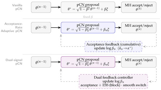
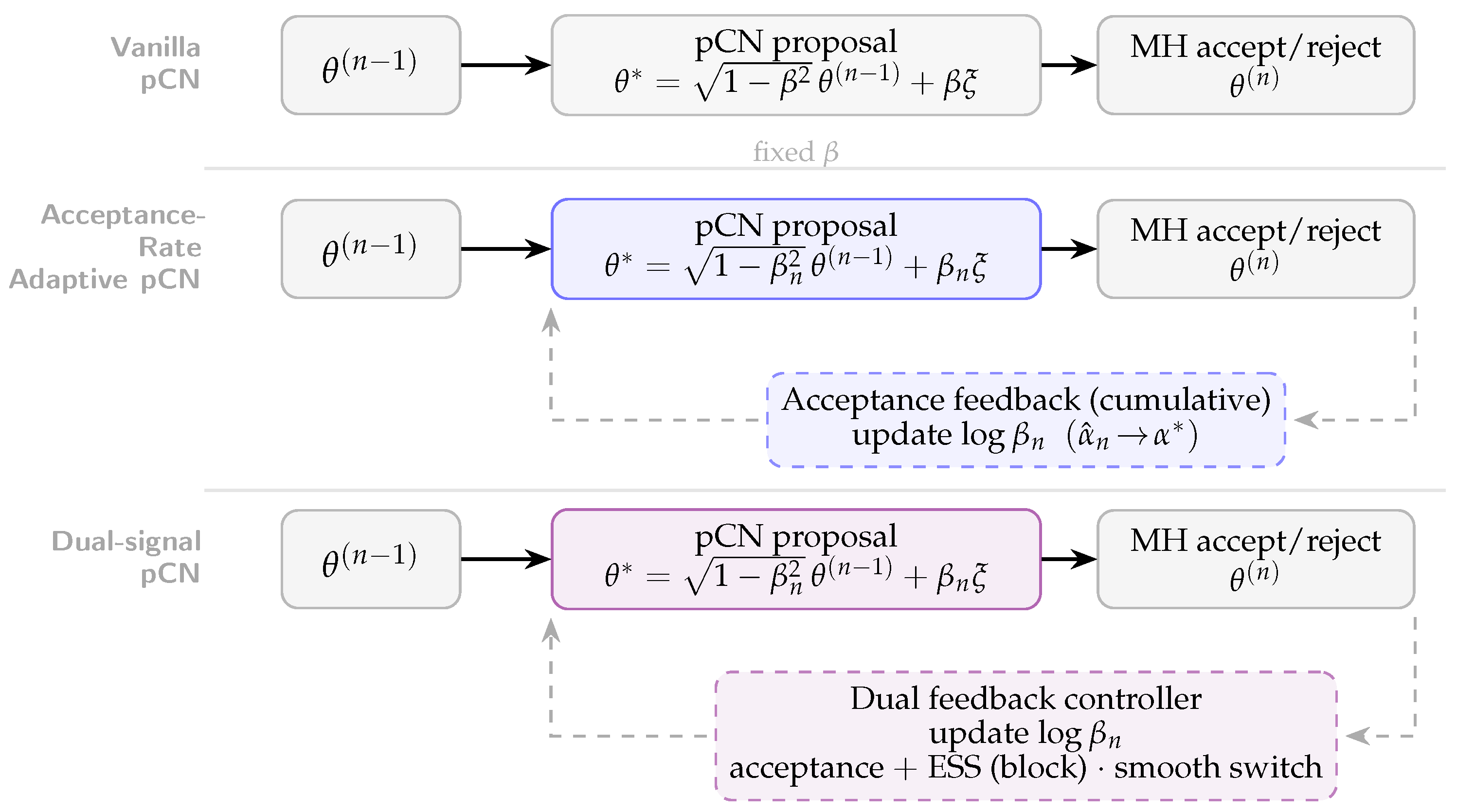
that gradually activates the ESS signal after sufficient samples have been collected. Figure 1 compares these three pCN variants.

Figure 1. Schematic comparison of three pCN variants. Vanilla pCN (gray) uses a fixed step size. Acceptance rate-adaptive (blue) adjusts ${\beta }_n$ via acceptance feedback during burn-in, while dual-signal pCN (purple) adds ESS feedback. Solid arrows denote sampling; dashed elements indicate burn-in adaptation mechanisms.

As in the single-signal variant, adaptation is confined to burn-in and then frozen. Although the dual-signal controller offers a flexible framework for incorporating efficiency diagnostics, the numerical experiments in Section 4 show that its additional benefits are problem-dependent and do not consistently surpass those of the acceptance rate-adaptive scheme. We therefore recommend the acceptance rate-adaptive pCN as the primary practical variant, and regard the dual-signal extension as an exploratory investigation of efficiency-aware feedback that may benefit specific problem classes warranting further study.

2.5. Comparison Methods: Adaptive Metropolis and MALA

We included two well-established MCMC algorithms as comparison baselines: adaptive Metropolis (AM) [18] and the Metropolis-adjusted Langevin algorithm (MALA) [14,26]. These methods employ fundamentally different adaptation strategies and proposal constructions, providing a broad basis for comparison.

The AM algorithm adapts the proposal covariance to the empirical posterior geometry observed during sampling. At iteration n, the proposal is drawn from

$${\theta }^{*}\sim \mathcal{N}\left({\theta }^{(n-1)},s_d{C}_n+s_dϵI_d\right),$$

(10)

where $C_n$ is the running empirical covariance of the chain history, $s_d=2.{38}^2/d$ is the dimension-dependent scaling factor derived from optimal scaling theory [19], and $ϵ>0$ is a small regularization constant ensuring positive definiteness. The covariance $C_n$ is updated incrementally using Welford’s algorithm after a delayed adaptation period (here, the first $10\%$ of burn-in uses a fixed prior-proportional proposal to stabilize early covariance estimates). The AM proposal is symmetric, so the MH acceptance ratio reduces to the standard likelihood–prior ratio. After burn-in, the covariance is frozen and the retained chain is a standard random-walk Metropolis kernel.

The MALA constructs gradient-informed proposals by discretizing the Langevin diffusion $d\theta ={\nabla }_{\theta }log\pi (\theta \mid y)dt+\sqrt{2}d{W}_t$. The proposal at step size h is

$${\theta }^{*}={\theta }^{(n-1)}+{\displaystyle \frac{h}{2}}{\nabla }_{\theta }log\pi ({\theta }^{(n-1)}\mid y)+\sqrt{h}Z,Z\sim \mathcal{N}(0,I_d),$$

(11)

with an MH correction to ensure detailed balance. For the linear-Gaussian benchmarks, exact gradients are available analytically; for the CQNLSE problem, we approximated gradients via forward finite differences with perturbation $\delta ={10}^{-4}$. The step size h was adapted during burn-in using the same Robbins–Monro scheme as the acceptance rate-adaptive pCN, targeting ${\alpha }^{*}=0.234$ (the same target rate as the pCN variants for consistency [26]). Gradient and drift terms were clipped to prevent proposal instability in regions of high curvature.

2.6. Unified Computational Framework

We implemented all five methods (vanilla pCN, acceptance rate-adaptive pCN, dual-signal pCN, AM, and MALA) within a common code structure. The three pCN variants share the same prior-preserving proposal and MH correction while isolating the variant-specific adaptation logic during burn-in; the AM and MALA use their respective proposal mechanisms (Equations (10) and (11)) under the same burn-in/freeze protocol.

Vanilla pCN uses a fixed step size, the acceptance rate-adaptive variant updates ${\beta }_n$ via cumulative acceptance feedback, and the dual-signal extension further incorporates a block-based ESS signal with smooth switching. The AM adapts its proposal covariance, and the MALA employs gradient-driven proposals with an adaptive step size. All variants use identical initialization, burn-in fraction, and post-burn-in freezing; their differences lie solely in the proposal and adaptation mechanism.

Algorithm 1 formalizes this workflow, parameterized by a variant flag V. By restricting adaptation to the burn-in and applying projection-bounded updates, the implementation preserves the ergodicity of the retained samples under standard regularity conditions while enabling straightforward switching between variants.

All details needed to replicate Algorithm 1 are as follows: the adaptation-update formulas appear in Equations (7) and (8); the complete set of hyperparameters (${\alpha }^{*}$, ${\gamma }_n$, K, $N_{\mathrm{burn}}$, projection bounds, initial step size, and dual-signal parameters) is listed in Table 1 with per-parameter justification; and the open-source code is available at https://github.com/cook-55/Ad-Pre-CN-MCMC-for-HD-BIP-main/tree/main (accessed on 1 July 2026).

Algorithm 1 Unified MCMC framework with variant-specific proposals and burn-in adaptation

Require: Forward operator $\mathcal{G}$, data y, noise variance ${\sigma }^2$, prior covariance ${\Sigma }_{\mathrm{prior}}$ Require: Variant flag $V\in \{\mathtt{Vanilla},\mathtt{AcceptanceRate},\mathtt{Dual},\mathtt{AM},\mathtt{MALA}\}$ Ensure: Posterior samples ${\left\{{\theta }^{\left(n\right)}\right\}}_{n=N_{\mathrm{burn}}+1}^{N_{\mathrm{total}}}$     1: Initialize ${\theta }^{\left(0\right)}$, $\beta \leftarrow {\beta }_0$ (or $h\leftarrow h_0$ for MALA), accepted count $a\leftarrow 0$     2: for $n=1$ to $N_{\mathrm{total}}$ do     3:    Proposal:     4:    if $V\in \{\mathtt{Vanilla},\mathtt{AcceptanceRate},\mathtt{Dual}\}$ then     5:       Draw $\xi \sim \mathcal{N}(0,{\Sigma }_{\mathrm{prior}})$;    ${\theta }^{*}\leftarrow \sqrt{1-{\beta }^2}{\theta }^{(n-1)}+\beta \xi$     6:    else if $V=\mathtt{AM}$ then     7:       ${\theta }^{*}\sim \mathcal{N}({\theta }^{(n-1)},s_d{C}_n+s_dϵI_d)$     8:    else if $V=\mathtt{MALA}$ then     9:       ${\theta }^{*}\leftarrow {\theta }^{(n-1)}+{\displaystyle \frac{h}{2}}\nabla log\pi \left({\theta }^{(n-1)}\right|y)+\sqrt{h}Z$,    $Z\sim \mathcal{N}(0,I_d)$   10:    end if   11:    MH step:   12:    if $logu<min(0,log\pi ({\theta }^{*}\mid y)-log\pi ({\theta }^{(n-1)}\mid y))$ then   13:       ${\theta }^{\left(n\right)}\leftarrow {\theta }^{*}$; $a\leftarrow a+1$   14:    else   15:       ${\theta }^{\left(n\right)}\leftarrow {\theta }^{(n-1)}$   16:    end if   17:    Adaptation (only during burn-in):   18:    if $V=\mathtt{Vanilla}$ or $n>N_{\mathrm{burn}}$ then   19:       Parameters frozen   20:    else if $nmodK=0$ then   21:       if $V=\mathtt{AcceptanceRate}$ then   22:          Update $\beta$ using acceptance rate feedback   23:       else if $V=\mathtt{Dual}$ then   24:          Update $\beta$ using combined acceptance rate and ESS feedback with logistic switching   25:       else if $V=\mathtt{AM}$ then   26:          Update running covariance $C_n$ (Welford); scale $s_d$ fixed   27:       else if $V=\mathtt{MALA}$ then   28:          Update step size h using acceptance rate feedback   29:       end if   30:    end if   31: end for

Table 1. Complete specification of algorithmic hyperparameters for all five methods.

Hyperparameter	Symbol	pCN Variants	AM	MALA
Target acceptance rate	${\alpha }^{*}$	0.234 (LG), 0.23 (CQNLSE)	—	0.234
RM gain sequence	${\gamma }_n$	$0.12/\sqrt{n_u+1}$ (LG)	—	$0.12/\sqrt{n_u+1}$
		$0.10/\sqrt{n_u+1}$ (CQNLSE)		$0.10/\sqrt{n_u+1}$
Update interval	K	200 (LG), 50 (CQNLSE)	1	200 (LG), 50 (CQNLSE)
Burn-in length	$N_{\mathrm{burn}}$	6000 (30%)/1500 (25%)	same	same
Projection bounds	$[{\beta }_{min},{\beta }_{max}]$	$[0.004,0.90]/\sqrt{d}$ (LG)	—	$[0.004,0.90]/\sqrt{d}$
		$[0.01,0.80]/\sqrt{d}$ (CQNLSE)		$[0.01,0.80]/\sqrt{d}$
Initial step size	${\beta }_0$/$h_0$	$0.2/\sqrt{d}$(LG), $0.5/\sqrt{d}$(CQNLSE)	—	$0.2/\sqrt{d}$/$0.5/\sqrt{d}$
AM scaling	$s_d$	—	$2.{38}^2/d$	—
AM regularization	$ϵ$	—	${10}^{-6}$	—
AM delayed start	—	—	$10\%$ burn-in	—
ESS block size (dual)	$B_{\mathrm{ess}}$	2000 (LG), 500 (CQNLSE)	—	—
ESS activation threshold	—	$n>2500$/$n>500$	—	—
Logistic switch midpoint	$t_{\mathrm{switch}}$	$0.5N_{\mathrm{burn}}$/2000	—	—
Logistic switch steepness	c	0.2	—	—
MALA gradient clip	—	—	—	${\parallel \nabla \parallel }_{\infty }\le {10}^3$
MALA FD perturbation (CQNLSE)	$\delta$	—	—	${10}^{-4}$
Number of chains	—	4	4	4
Total evaluations	$N_{\mathrm{eval}}$	20,000 (LG), 6000 (CQNLSE)	same	same

3. Theoretical Analysis

The results in this section apply standard Markov chain theory to the freeze-after-burn-in design. They do not claim new mathematical properties of the adaptation mechanism; rather, they confirm that the proposed procedure preserves posterior consistency and characterize the conditional convergence rate of the frozen kernel, setting the stage for the empirical findings in Section 4.

3.1. Ergodicity

Both adaptive pCN variants employ a freeze-after-burn-in strategy: the step size $\beta$ is adapted only during a finite initial burn-in phase and held fixed thereafter. This design circumvents the main technical challenges of fully time-inhomogeneous adaptive MCMC algorithms, and allows asymptotic correctness to follow directly from classical MH theory.

Theorem 1

(Asymptotic correctness under finite adaptation). Let $\pi (\theta \mid y)$ be the posterior distribution defined in (3). For each fixed $\beta \in (0,1)$, let $P_{\beta }$ denote the Markov transition kernel of the pCN MH algorithm induced by the proposal

$${\theta }^{*}=\sqrt{1-{\beta }^2}\theta +\beta \xi ,\xi \sim \mathcal{N}(0,{\Sigma }_{\mathrm{prior}}),$$

together with the acceptance probability (5).

Consider an adaptive scheme that generates a sequence ${\left\{{\theta }^{\left(n\right)}\right\}}_{n\ge 0}$ along with step sizes ${\left\{{\beta }_n\right\}}_{n\ge 0}$ that may depend on the full history ${\theta }^{(0:n-1)}$. Suppose there exists a deterministic integer $N_{\mathrm{adapt}}<\infty$ such that

$${\beta }_n\equiv {\beta }^{★}:={\beta }_{N_{\mathrm{adapt}}}\mathit{for}\mathit{all}n\ge N_{\mathrm{adapt}},$$

where ${\beta }^{★}\in (0,1)$ is a random variable.

Then, conditional on the realized value of ${\beta }^{★}$, the tail chain ${\left\{{\theta }^{\left(n\right)}\right\}}_{n\ge N_{\mathrm{adapt}}}$ is a time-homogeneous Markov chain with transition kernel $P_{{\beta }^{★}}$. Moreover, for $\mathbb{P}$-almost every realization of ${\beta }^{★}$, the kernel $P_{{\beta }^{★}}$ is π-reversible and admits $\pi (·\mid y)$ as an invariant distribution.

If, in addition, $P_{{\beta }^{★}}$ is π-irreducible, aperiodic, and Harris recurrent, then

$$\underset{n\to \infty }{lim}{∥\mathcal{L}\left({\theta }^{(N_{\mathrm{adapt}}+n)}\right)-\pi (·\mid y)∥}_{\mathrm{TV}}=0,\mathit{almost}\mathit{surely}.$$

(12)

Proof. 

Fix any $\beta \in (0,1)$. The pCN proposal is reversible with respect to the Gaussian prior measure. Combined with the MH correction targeting $\pi (·\mid y)$, the resulting kernel $P_{\beta }$ satisfies detailed balance and therefore admits $\pi (·\mid y)$ as an invariant distribution [6,28].

By the finite adaptation assumption, the step size is constant after time $N_{\mathrm{adapt}}$. Hence, conditional on the realized value of ${\beta }^{★}$, the post-adaptation process evolves according to the time-homogeneous kernel $P_{{\beta }^{★}}$. Under $\pi$-irreducibility, aperiodicity, and Harris recurrence, standard Markov chain theory yields convergence to stationarity in total variation, which proves (12). □

Remark 1.

Theorem 1 applies directly to the acceptance rate-adaptive pCN and its dual-signal extension, since both restrict adaptation to a finite burn-in phase and freeze the step size thereafter. Asymptotic correctness thus follows from classical time-homogeneous Markov chain theory without requiring diminishing adaptation or containment conditions.

3.2. Post-Adaptation Convergence Rate

We next state a standard quantitative convergence result for the frozen pCN kernel, which characterizes the convergence speed in the post-burn-in phase.

Theorem 2

(Post-adaptation convergence rate under a spectral gap). Assume the setting of Theorem 1. Suppose that, for $\mathbb{P}$-almost every realization of ${\beta }^{★}$, the frozen kernel $P_{{\beta }^{★}}$ is π-reversible and possesses a nonzero $L^2\left(\pi \right)$ spectral gap $\lambda \left({\beta }^{★}\right)\in (0,1]$, that is,

$$\parallel P_{{\beta }^{★}}{f\parallel }_{L^2\left(\pi \right)}\le (1-\lambda \left({\beta }^{★}\right)){\parallel f\parallel }_{L^2\left(\pi \right)}\mathit{for}\mathit{all}f\in L_0^2\left(\pi \right),$$

(13)

where $L_0^2\left(\pi \right)$ denotes the subspace of mean-zero functions under π.

Then, for any initial distribution $\nu \ll \pi$ with the Radon–Nikodym derivative ${\displaystyle \frac{d\nu }{d\pi }}\in L^2\left(\pi \right)$, the post-burn-in chain satisfies

$${∥\nu P_{{\beta }^{★}}^n-\pi ∥}_{\mathrm{TV}}\le {\displaystyle \frac{1}{2}}{∥{\displaystyle \frac{d\nu }{d\pi }}-1∥}_{L^2\left(\pi \right)}{(1-\lambda \left({\beta }^{★}\right))}^n,n\ge 0,$$

(14)

for $\mathbb{P}$-almost every realization of ${\beta }^{★}$.

Proof. 

For $\mathbb{P}$-almost every realization of ${\beta }^{★}$, reversibility implies that $P_{{\beta }^{★}}$ is self-adjoint on $L^2\left(\pi \right)$. The spectral gap assumption yields geometric contraction on $L_0^2\left(\pi \right)$. Let $h={\displaystyle \frac{d\nu }{d\pi }}-1\in L_0^2\left(\pi \right)$. Then,

$$\parallel P_{{\beta }^{★}}^n{h\parallel }_{L^2\left(\pi \right)}\le {(1-\lambda \left({\beta }^{★}\right))}^n{\parallel h\parallel }_{L^2\left(\pi \right)}.$$

Finally, the standard inequality ${\parallel \mu -\pi \parallel }_{\mathrm{TV}}\le {\displaystyle \frac{1}{2}}{\parallel {\displaystyle \frac{d\mu }{d\pi }}-1\parallel }_{L^2\left(\pi \right)}$ yields (14). □

Remark 2.

Theorem 2 shows that the post-burn-in convergence speed depends on the spectral properties of the frozen kernel, conditional on the existence of a nonzero spectral gap. The adaptation therefore aims to select a step size ${\beta }^{★}$ that improves practical mixing based on acceptance rate feedback. Although we did not prove that adaptation enlarges the spectral gap for every target, the empirical results in Section 4 show that the adapted step sizes consistently yield improved the ESS and convergence diagnostics. Explicit lower bounds on $\lambda \left(\beta \right)$ are problem-dependent, and determining whether $\lambda \left({\beta }^{★}\right)>\lambda \left({\beta }_{\mathrm{manual}}\right)$ in general is a topic for future work.

3.3. Monte Carlo Consistency of Ergodic Averages

We finally confirmed the Monte Carlo consistency of the empirical averages computed from the retained samples.

Corollary 1

(Strong law of large numbers). Assume the setting of Theorem 1. Let $f:{\mathbb{R}}^d\to \mathbb{R}$ be measurable with ${\mathbb{E}}_{\pi }\left[\right|f\left|\right]<\infty$. Then, for $\mathbb{P}$-almost every realization of ${\beta }^{★}$,

$$\underset{N\to \infty }{lim}{\displaystyle \frac{1}{N}}{\displaystyle \sum _{n=N_{\mathrm{adapt}}+1}^{N_{\mathrm{adapt}}+N}}f\left({\theta }^{\left(n\right)}\right)=\int f\left(\theta \right)\pi (\theta \mid y)d\theta \mathit{almost}\mathit{surely}.$$

(15)

Proof. 

For $\mathbb{P}$-almost every realization of ${\beta }^{★}$, the post-adaptation chain is time-homogeneous with invariant distribution $\pi$. Under $\pi$-irreducibility, aperiodicity, and Harris recurrence, the Markov chain ergodic theorem yields the strong law of large numbers for any $\pi$-integrable function f. □

Corollary 1 rigorously justifies using post-burn-in samples for estimating posterior expectations, variances, and credible intervals. The statistical efficiency of such estimators is governed by the integrated autocorrelation time, which is commonly summarized using the ESS.

Remark 3.

The results above confirm that the freeze-after-burn-in adaptive pCN framework retains detailed balance, the correct invariant distribution, and ergodic convergence. Confining adaptation to a finite burn-in window preserves the analytical tractability of time-homogeneous kernels while allowing for fully automated, data-driven step-size selection. The transient adaptation dynamics during burn-in, governed by stochastic approximation theory, are a topic for future study.

4. Numerical Experiments

All comparisons followed the diagnostic definitions and computational budget constraints described in Section 4.1.

4.1. Experimental Design and Evaluation Metrics

Each experiment used a fixed computational budget: 20,000 log-posterior evaluations per chain for the linear-Gaussian benchmarks and 6000 evaluations per chain for the CQNLSE benchmark. Four independent parallel chains were run for each configuration, initialized by a small Gaussian perturbation around the maximum a posteriori estimate:

$${\theta }^{\left(0\right)}\sim \mathcal{N}\left({\theta }_{\mathrm{MAP}},c_0^2\mathrm{diag}\left({\Sigma }_{\mathrm{prior}}\right)\right),$$

(16)

where $c_0=0.05$ for the linear-Gaussian experiments and $c_0=0.1$ for the CQNLSE benchmark.

Thirty percent of the budget was allocated to burn-in for linear-Gaussian experiments (6000 iterations), while 25% (1500 iterations) was used for the CQNLSE benchmark. During the burn-in, the adaptive controllers may update the step size $\beta$; after burn-in, adaptation is terminated and $\beta$ is frozen. The retained samples are thus generated by a time-homogeneous pCN MH kernel targeting the posterior $\pi (\theta \mid y)$.

We compared five methods: vanilla pCN with a fixed step size $\beta$ throughout sampling; acceptance rate-adaptive pCN, which performs periodic Robbins–Monro updates of $log\beta$ based on the cumulative acceptance rate feedback; dual-signal pCN, which augments the acceptance rate feedback with an auxiliary ESS signal activated gradually via a logistic switching schedule; the adaptive Metropolis (AM), which adapts the full proposal covariance using Welford’s incremental algorithm with delayed adaptation; and the Metropolis-adjusted Langevin algorithm (MALA), which uses gradient-informed proposals with an adaptive step size. All algorithmic hyperparameters are explicitly reported in Table 1 and justified below.

The performance was assessed on the post-burn-in samples aggregated across the four chains using the following metrics:

• Split-$\widehat{R}$ convergence diagnostic [29]: Each chain is split into two halves to form eight segments. Let W and B denote the within- and between-segment variances. The potential scale reduction factor is

  $$\widehat{R}=\sqrt{{\displaystyle \frac{\widehat{V}}{W}}},\widehat{V}={\displaystyle \frac{n_2-1}{n_2}}W+{\displaystyle \frac{1}{n_2}}B,$$

  (17)

  where $n_2$ is the segment length. We report the maximum $\widehat{R}$ across all coordinates.
• ESS: For each coordinate, the integrated autocorrelation time $\widehat{\tau }$ is estimated as $1+2{\sum }_{k=1}^L{\widehat{\rho }}_k$, truncated at the first negative autocorrelation or a prescribed maximum lag. Then,

  $$\mathrm{ESS}={\displaystyle \frac{n_{\mathrm{post}}}{max(\widehat{\tau },{10}^{-12})}}.$$

  (18)
  We report both the mean and minimum ESS across coordinates.
• Normalized efficiency:

  $$\mathrm{ESS}/\mathrm{eval}={\displaystyle \frac{\mathrm{ESS}}{N_{\mathrm{eval}}}},\mathrm{ESS}/\sec ={\displaystyle \frac{\mathrm{ESS}}{T_{\mathrm{wall}}}},$$

  (19)

  where $N_{\mathrm{eval}}$ and $T_{\mathrm{wall}}$ denote the total number of log-posterior evaluations and the wall-clock time, respectively.
• Posterior estimation accuracy (linear-Gaussian cases only): the relative ${\ell }_2$ error of the posterior mean (${\mathrm{Err}}_{\mu }$), the relative Frobenius norm error of the posterior covariance (${\mathrm{Err}}_{\Sigma }$), and the trace contraction ratio $\mathrm{Tr}\left(\widehat{\Sigma }\right)/\mathrm{Tr}\left({\Sigma }_{\mathrm{true}}\right)$.

All runs used identical random seeds and hardware. Numerical safeguards included variance flooring and ESS clipping to $[1,n_{\mathrm{post}}]$. All the reported performance metrics (ESS, ESS/eval, ESS/sec, and split-$\widehat{R}$) were computed as the means across the four independent chains. The chain-to-chain variability was quantified by the split-$\widehat{R}$ diagnostic, which captures both within-chain and between-chain discrepancies; values close to 1.0 indicate that all chains explore the same posterior region consistently.

4.1.1. Hyperparameter Specification and Justification

Table 1 provides a complete listing of all algorithmic hyperparameters for both the linear-Gaussian and CQNLSE experiments. Each choice is briefly justified below.

The target acceptance rate was set to ${\alpha }^{*}=0.234$, following the classical optimal scaling result for random-walk Metropolis algorithms in high dimensions [19], which establishes that an acceptance rate near $0.234$ maximizes the expected squared jumped distance under Gaussian targets. For the two-dimensional CQNLSE problem, we used ${\alpha }^{*}=0.23$ as a minor practical adjustment.

For the Robbins–Monro gain sequence, the gain ${\gamma }_n=c_{\gamma }/\sqrt{n_u+1}$ (where $n_u$ counts the number of updates so far) satisfies the standard Robbins–Monro conditions $\sum {\gamma }_n=\infty$, $\sum {\gamma }_n^2<\infty$, ensuring that adaptation diminishes over time while retaining sufficient responsiveness during burn-in. The prefactors ($0.12$ and $0.10$) were selected to yield moderate step-size adjustments that avoid overshooting during early exploration.

The update interval was set to $K=200$ iterations for the linear-Gaussian experiments and $K=50$ for CQNLSE. The larger interval for the linear-Gaussian case ensures that the cumulative acceptance rate has stabilized between updates, while the shorter interval for the low-dimensional CQNLSE problem permits more responsive adaptation.

Regarding the burn-in length, a 30% burn-in for the linear-Gaussian experiments provides ample adaptation time across dimensions up to $d=100$. The 25% burn-in for CQNLSE is sufficient given the low dimensionality ($d=2$) and shorter total chain length.

The projection bounds $[a/\sqrt{d},b/\sqrt{d}]$ reflect the well-known optimal scaling $\beta \sim d^{-1/2}$ for pCN-like proposals. The constants a and b prevent degenerate step sizes (too small or too large) and are set conservatively.

For the dual-signal parameters, the ESS block size determines the window over which autocorrelation-based efficiency is estimated; larger blocks yield more stable estimates, but delay the signal. The logistic switching midpoint $t_{\mathrm{switch}}$ is set near the middle of the burn-in so that the ESS signal is activated only after the acceptance rate controller has brought $\beta$ into a reasonable range.

4.1.2. Sensitivity to Hyperparameter Choices

We note that the proposed adaptation scheme was designed to be robust to moderate variations in its hyperparameters. The Robbins–Monro gain sequence diminishes as $O\left(n_u^{-1/2}\right)$, so the final adapted step size is determined primarily by the cumulative acceptance rate trajectory rather than by the initial gain magnitude. The target acceptance rate ${\alpha }^{*}=0.234$ is grounded in optimal scaling theory, and small perturbations (e.g., ${\alpha }^{*}\in [0.20,0.30]$) produce qualitatively similar behavior in preliminary tests. The projection bounds prevent pathological step sizes, regardless of the other settings. The burn-in length and update interval jointly determine the total number of adaptation steps; as long as this number is sufficiently large (here, ≥30 updates for the linear-Gaussian case and ≥29 for CQNLSE), the Robbins–Monro procedure has adequate opportunity to converge. These design choices collectively ensure that the observed improvements are not attributable to a single favorable tuning configuration, but rather reflect the general benefit of systematic acceptance rate feedback over fixed manual step sizes.

4.2. Benchmark Problems

The methods were evaluated on two complementary classes of benchmarks.

4.2.1. Linear-Gaussian Inverse Problems with Controlled Spectral Structure

These benchmarks take the form $y=A\theta +\eta$, where the forward operator A is constructed via randomized singular value decomposition with a prescribed condition number and a heterogeneous diagonal Gaussian prior is imposed. This setup allows for systematic variation in the dimension ($d=10$ to 100), conditioning ($\kappa =2$ to 200), and signal-to-noise ratio (from $-9$ dB to $+8$ dB). The five regimes are summarized in Table 2.

Table 2. Synthetic experimental regimes for the linear-Gaussian benchmark. All use 20,000 evaluations per chain and four parallel chains.

Experiment	Dimension	Condition Number	SNR (dB)	Purpose
BaselineScan	10–100	20	0	Dimension scaling under fixed conditioning
WellConditioned	80	2	0	Mild anisotropy reference
IllConditioned	80	200	0	Stress test for stiff posterior directions
LowSNR	80	20	$-9$	Weak likelihood information
HighSNR	80	20	$+8$	Sharp posterior dominated by data

4.2.2. Nonlinear Wave Propagation: CQNLSE

The second benchmark identifies coefficients $(\alpha ,\beta )$ in the CQNLSE. This low-dimensional ($d=2$) nonlinear problem serves as a proof of concept for the proposed adaptive methods on non-Gaussian posteriors with PDE-constrained forward operators, rather than as a test of high-dimensional scalability:

$$i{\partial }_{t}u+{\displaystyle \frac{1}{2}}{\partial }_{xx}u+{\alpha \left|u\right|}^{2}u+\beta {\left|u\right|}^{4}u=0,$$

with initial condition $u(x,0)=1.5\mathrm{sech}\left(x\right)$. Forward simulations use a second-order split-step Fourier method. The resulting posterior is non-Gaussian and exhibits strong anisotropy and parameter coupling. The numerical configuration is summarized in Table 3.

Table 3. Numerical configuration for the CQNLSE inverse problem.

Category	Parameter	Setting
Forward model	Governing equation	CQNLSE
	Initial condition	$u(x,0)=1.5\mathrm{sech}\left(x\right)$
	Final time	$T=0.5$
	Spatial grid	64 points, periodic domain
	Time stepping	100 split-step Fourier steps
	Observation noise	Complex Gaussian, ${\sigma }_{\mathrm{obs}}=0.02$
Unknown parameters	True coefficients	${\alpha }^{†}=1.0$, ${\beta }^{†}=0.1$
	Prior on $\alpha$	$\mathcal{N}(0.8,{0.2}^2)$
	Prior on $\beta$	$\mathcal{N}(0.2,{0.1}^2)$
MCMC configuration	Dimension	$d=2$
	Total iterations	6000
	Burn-in	1500
	Adaptation interval	Every 50 steps

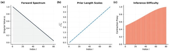
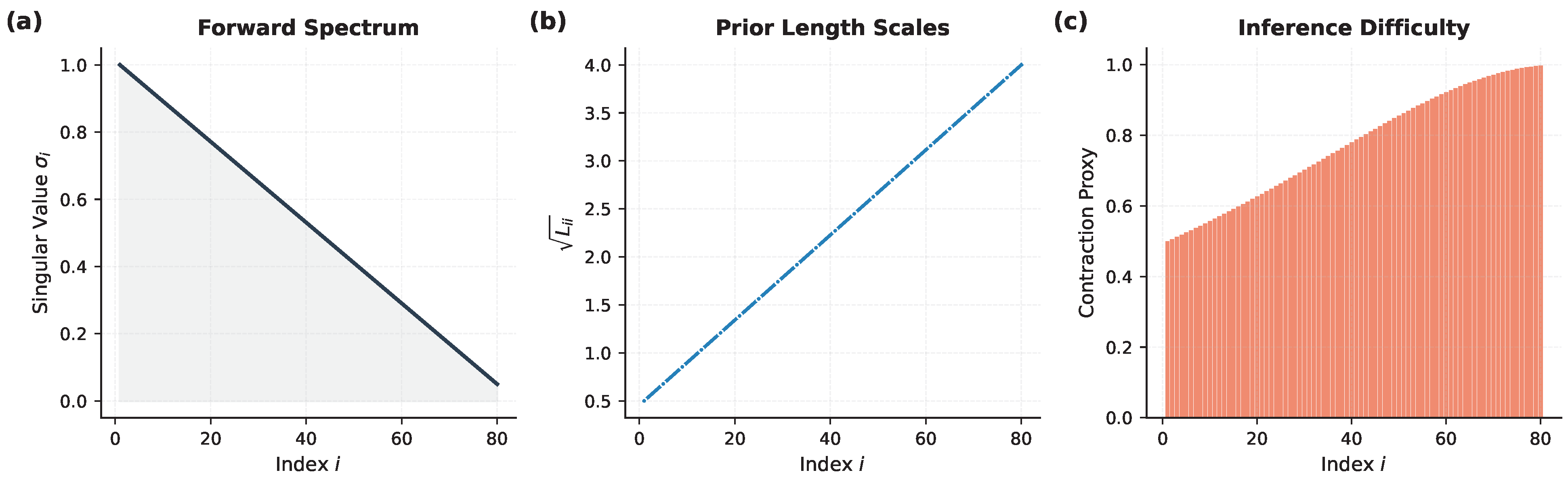
Figure 2 provides a visual overview of the linear-Gaussian benchmark design, illustrating the forward operator spectrum, the prior length scales, and the resulting inference difficulty across different conditioning regimes.

Figure 2. Problem setup for the linear-Gaussian benchmarks. (a) Singular value spectrum of the forward operator showing controlled decay. (b) Prior length scales across dimensions. (c) Inference difficulty as measured by the posterior contraction ratio across regimes.

4.3. Results for Linear-Gaussian Benchmarks

Across all linear-Gaussian regimes, the acceptance rate-adaptive pCN consistently outperformed vanilla pCN in the ESS and convergence diagnostics, while also yielding an improved posterior estimation accuracy in most cases. Among the comparison methods, the adaptive Metropolis (AM) and MALA showed a competitive or superior ESS in several regimes, particularly under well-conditioned and low-SNR settings where the posterior geometry is more amenable to covariance-adapted and gradient-informed proposals. However, their advantages are less consistent in ill-conditioned and high-SNR regimes. The dual-signal pCN extension improves upon the baseline, although its gains are generally less consistent than those of the acceptance rate controller, particularly in ill-conditioned and low signal-to-noise regimes.

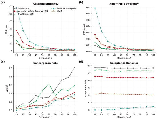
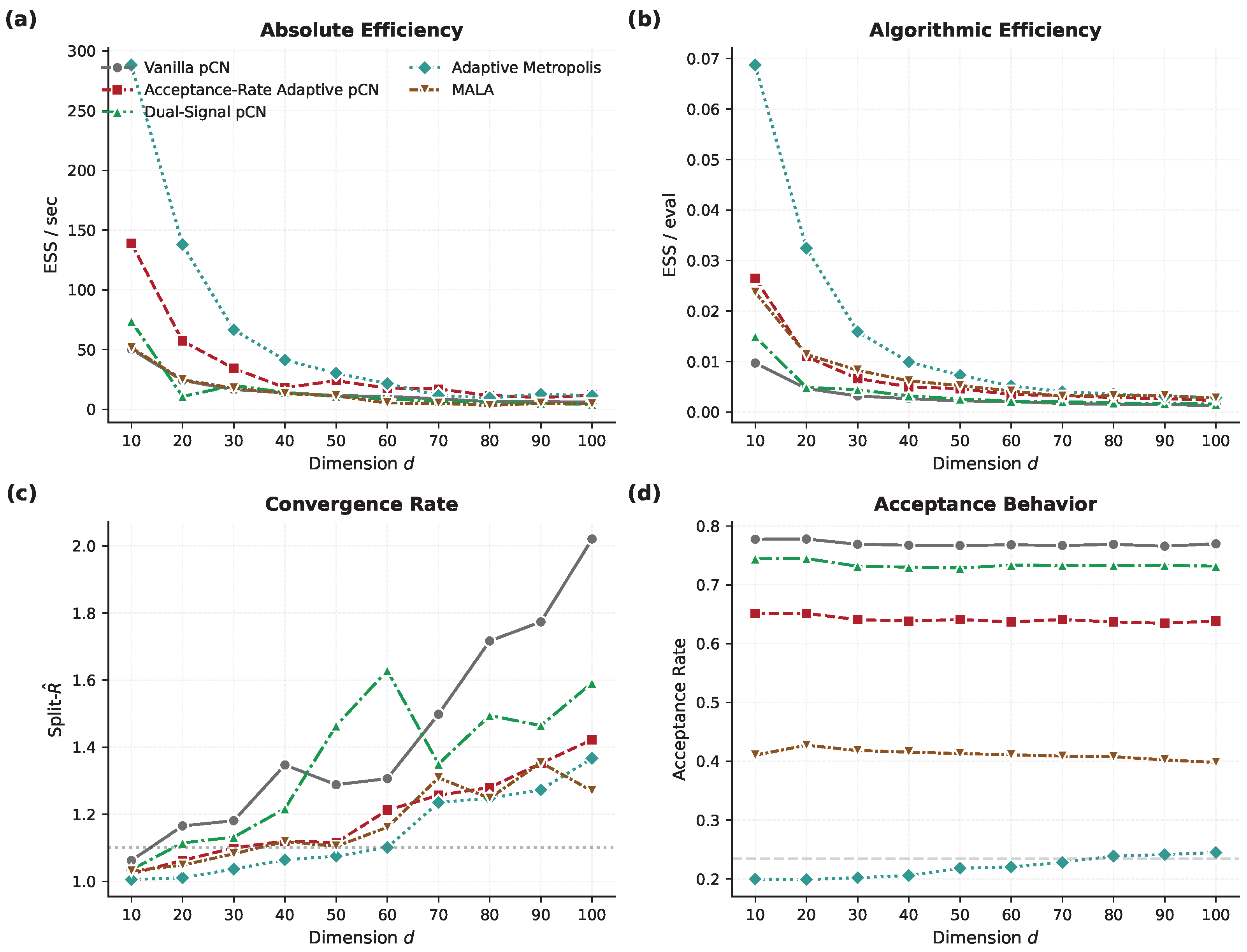
In the baseline dimension scaling sweep ($d=10$ to 100), the acceptance rate-adaptive pCN achieved the highest efficiency, as measured by the ESS per evaluation (Figure 3b). It also maintained a relatively better inter-chain agreement than vanilla pCN, as reflected by the slower growth of split-$\widehat{R}$ with dimension (Figure 3c). The AM and MALA exhibited distinct scaling behaviors: the AM benefits from covariance adaptation at moderate dimensions, but shows increasing computational overhead from the full-tensor covariance update, while the MALA’s gradient-driven proposals maintain a good ESS per evaluation, but require more wall-clock time per iteration. Vanilla pCN shows clear degradation in the convergence quality at higher dimensions, confirming the limitations of manual step-size tuning in moderate-dimensional settings.

Figure 3. Baseline dimension scaling comparison ($d=10$ to 100). (a) ESS per second. (b) ESS per evaluation. (c) Split-$\widehat{R}$. (d) Acceptance rate. The acceptance rate-adaptive pCN exhibited superior algorithmic efficiency and more stable convergence behavior across dimensions.

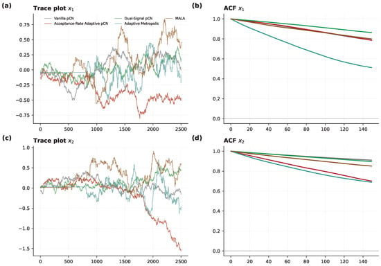
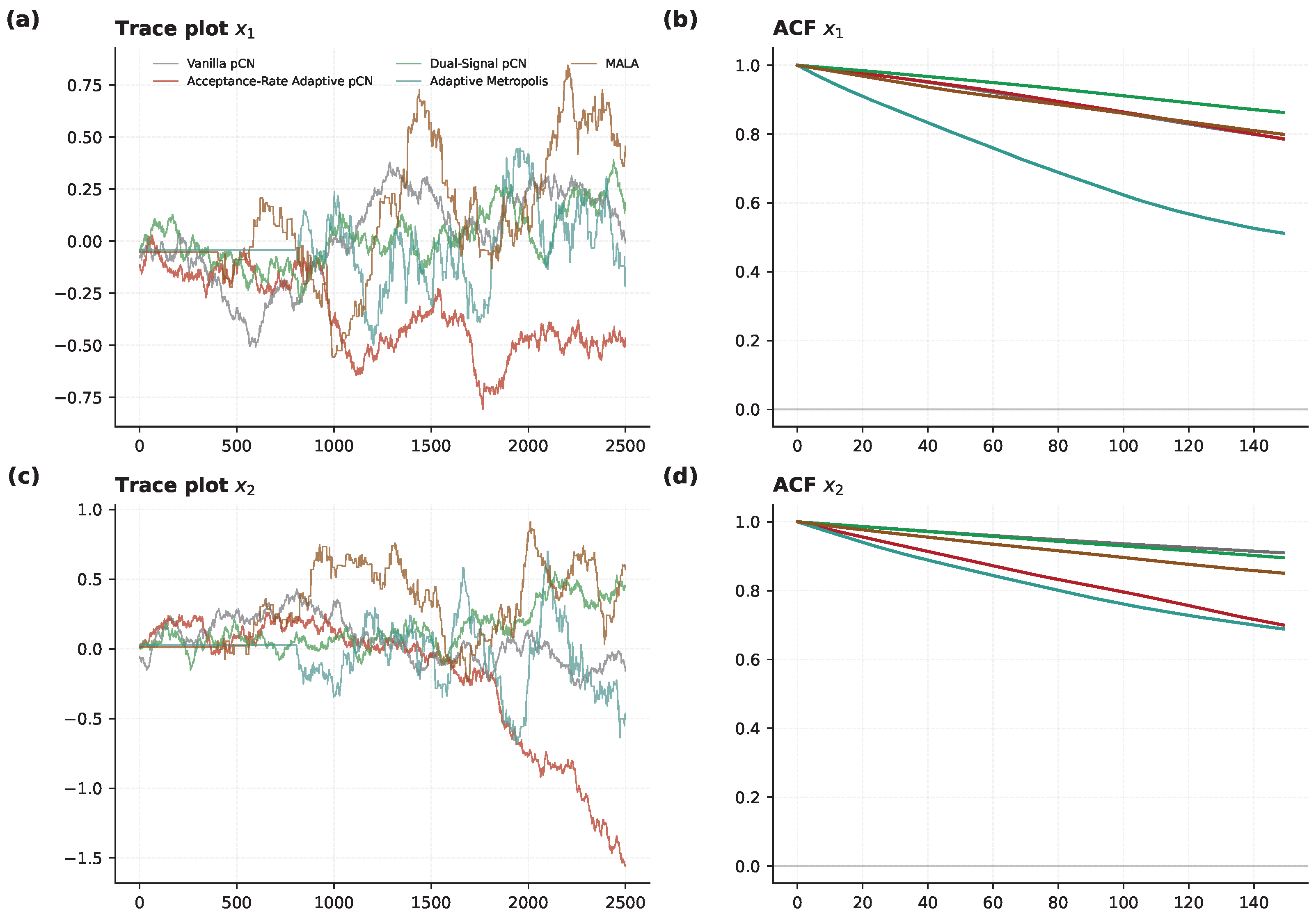
In the severely ill-conditioned regime ($\kappa =200$), the advantage of acceptance rate-adaptive pCN is most pronounced (Table 4 and Figure 4). It roughly doubles the ESS per evaluation relative to vanilla pCN and achieves a clear reduction in split-$\widehat{R}$, indicating significantly improved mixing under strong posterior anisotropy. The AM and MALA achieved comparable ESS/eval to the acceptance rate-adaptive pCN ($0.0030$ and $0.0029$ respectively, versus $0.0028$ for AR-adaptive pCN), and both achieved lower split-$\widehat{R}$ ($1.30$ and $1.29$) than vanilla pCN ($1.66$). However, the AM incurred a higher wall-clock time ($7.02$ s versus $3.80$ s) due to covariance matrix operations, and the MALA was substantially slower ($11.95$ s) due to gradient computation. Trace plots and autocorrelation functions confirmed that adaptive tuning reduces chain stickiness and accelerates decorrelation. The dual-signal pCN extension provides moderate improvement, but is outperformed by the acceptance-rate controller.

Table 4. Results in the ill-conditioned regime ($d=80$, $\kappa =200$, SNR = 0 dB).

Method	AR	ESS	ESS/eval	Split-$\widehat{\mathit{R}}$	ESS/s
Vanilla pCN	0.771	30.5	0.0015	1.655	7.92
Acceptance rate-adaptive pCN	0.645	56.4	0.0028	1.218	14.83
Dual-signal pCN	0.737	31.0	0.0015	1.546	4.86
Adaptive Metropolis	0.239	60.0	0.0030	1.304	8.54
MALA	0.408	57.9	0.0029	1.292	4.85

Figure 4. Trace plots and autocorrelation functions in the ill-conditioned regime for all five methods. (a) Trace plot for $x_1$; (b) autocorrelation function for $x_1$; (c) trace plot for $x_2$; (d) autocorrelation function for $x_2$. Adaptive tuning, particularly acceptance rate feedback, reduces stickiness and accelerates autocorrelation decay compared with vanilla pCN. AM and MALA show intermediate trace behavior, with MALA exhibiting higher autocorrelation at longer lags due to its smaller effective step size.

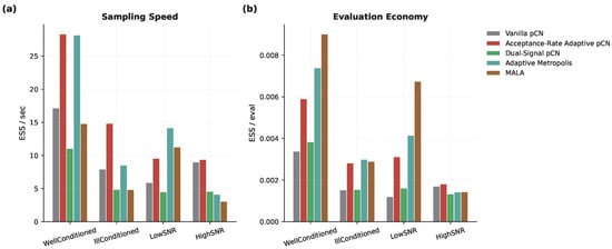
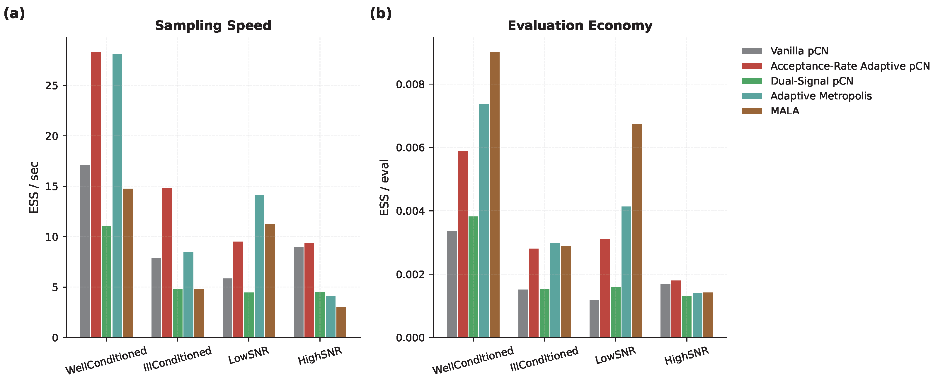
The robustness across conditioning and signal-to-noise ratio variations is summarized in Figure 5. The acceptance rate-adaptive pCN delivered the most consistent efficiency gains across all four regimes. The AM achieved the highest absolute ESS in the well-conditioned regime (ESS = 147.9) and low-SNR regime (ESS = 83.0), showing the benefit of covariance adaptation when the posterior geometry is relatively isotropic. The MALA excelled in the low-SNR regime (ESS = 134.9), where the likelihood is weak and gradient information helps guide the sampler, but underperformed in the high-SNR regime (ESS = 28.7), where the sharp posterior challenges the finite-difference gradient approximation. The dual-signal pCN showed the largest improvements in the ill-conditioned and low-SNR regimes, where fixed-step proposals struggled the most.

Figure 5. Efficiency comparison across regimes at fixed dimension ($d=80$) for all five methods. (a) ESS per second. (b) ESS per evaluation. The acceptance rate-adaptive pCN showed the most consistent gains, while the AM and MALA exhibited regime-dependent advantages.

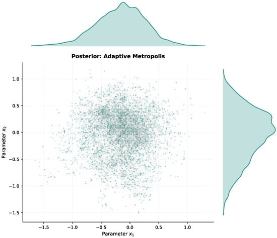
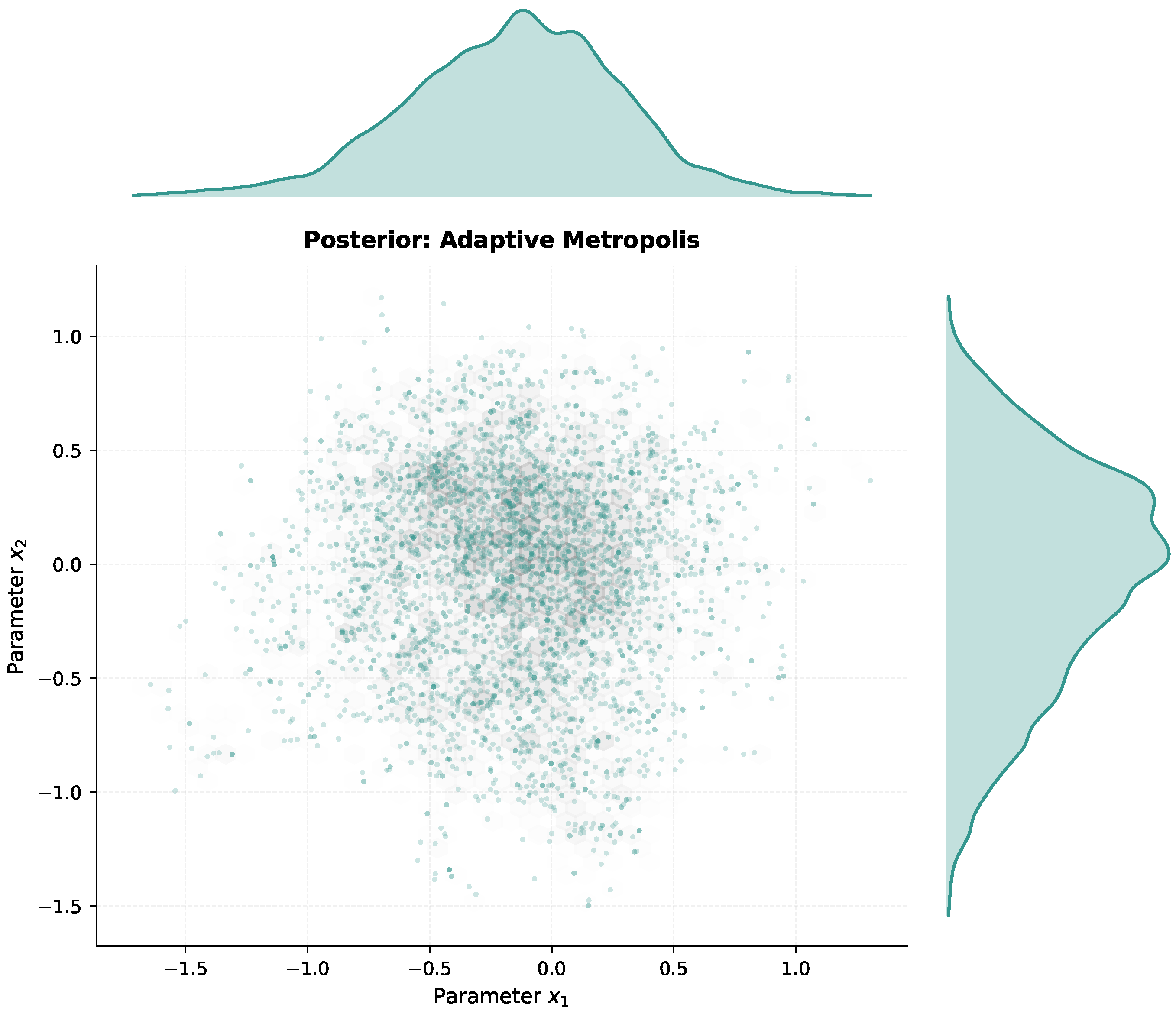
Figure 6 presents the posterior marginal distributions estimated by the AM in the ill-conditioned regime, illustrating the characteristic elliptical posterior geometry and the quality of the marginal approximations achieved by the adapted covariance proposal.

Figure 6. Posterior marginal distributions from the adaptive Metropolis in the ill-conditioned regime ($d=80$, $\kappa =200$). Joint posterior samples (left) and marginal histograms (diagonal) demonstrate that the adapted covariance approximates the posterior geometry.

4.4. Results for the CQNLSE Inverse Problem

Table 5 summarizes the performance of all five methods on the nonlinear benchmark. The adaptive Metropolis achieved the highest ESS (304.5) and the most accurate posterior mean estimates ($|{\alpha }_{\mathrm{err}}|=0.026$, $|{\beta }_{\mathrm{err}}|=0.009$), with favorable convergence diagnostics ($\widehat{R}=1.018$). This substantial improvement over the pCN variants likely stems from the adapted covariance capturing the strong parameter coupling in the two-dimensional CQNLSE posterior. Among the pCN methods, the acceptance rate-adaptive variant (ESS = 171.6) slightly outperformed vanilla pCN (ESS = 170.7) and dual-signal pCN (ESS = 145.0), though all three yielded reasonable convergence diagnostics ($\widehat{R}\le 1.036$). The MALA performed poorly in this implementation (ESS = 12.9, $\widehat{R}=1.49$). Since analytic or adjoint gradients were unavailable, we used finite differences, which require additional forward solves and may be inaccurate for the oscillatory CQNLSE model. This may put the MALA at a disadvantage, so the result should not be taken as a general limitation of the MALA with accurate gradients. We note that the pCN and AM results exhibit more favorable convergence diagnostics than the MALA, whose elevated $\widehat{R}$ indicates incomplete mixing within the allocated budget.

Table 5. Results for the CQNLSE inverse problem. True values are ${\alpha }^{†}=1.0$ and ${\beta }^{†}=0.1$.

Method	AR	ESS	$\widehat{\mathit{R}}$	$|{\mathit{\alpha }}_{\mathbf{err}}|$	$|{\mathit{\beta }}_{\mathbf{err}}|$
Vanilla pCN	0.029	170.7	1.011	0.050	0.019
Acceptance rate-adaptive pCN	0.049	171.6	1.036	0.051	0.020
Dual-signal pCN	0.058	145.0	1.019	0.049	0.019
Adaptive Metropolis	0.307	304.5	1.018	0.026	0.009
MALA	0.172	12.9	1.490	0.044	0.017

We caution that the posterior mean estimates and credible intervals for the CQNLSE problem should be interpreted with care, as the convergence diagnostics vary across methods and complete convergence may not have been achieved within the allocated computational budget.

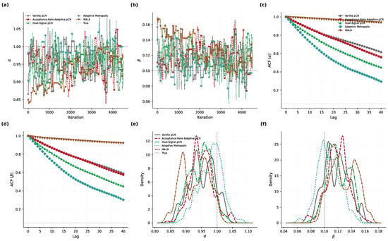
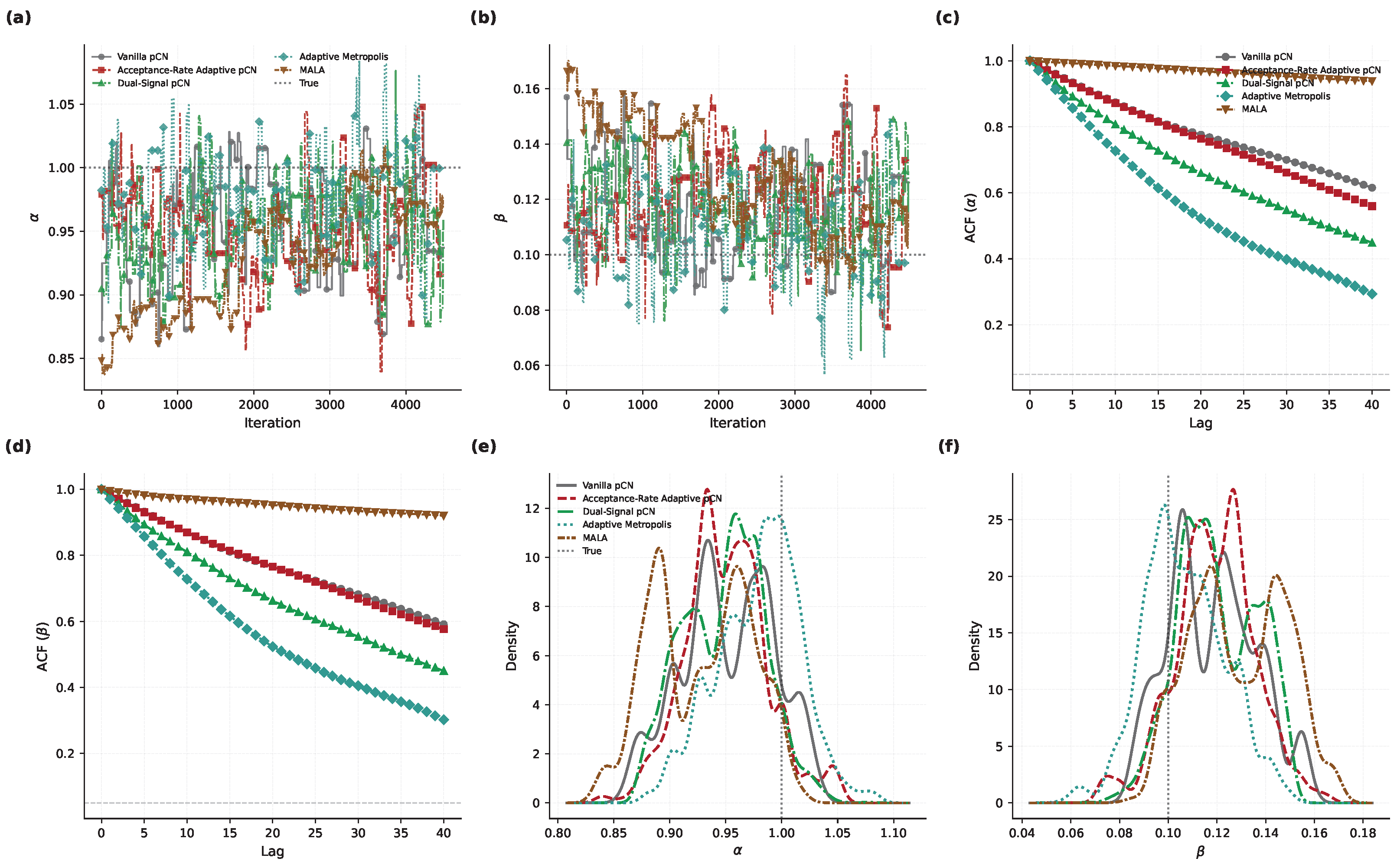
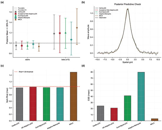
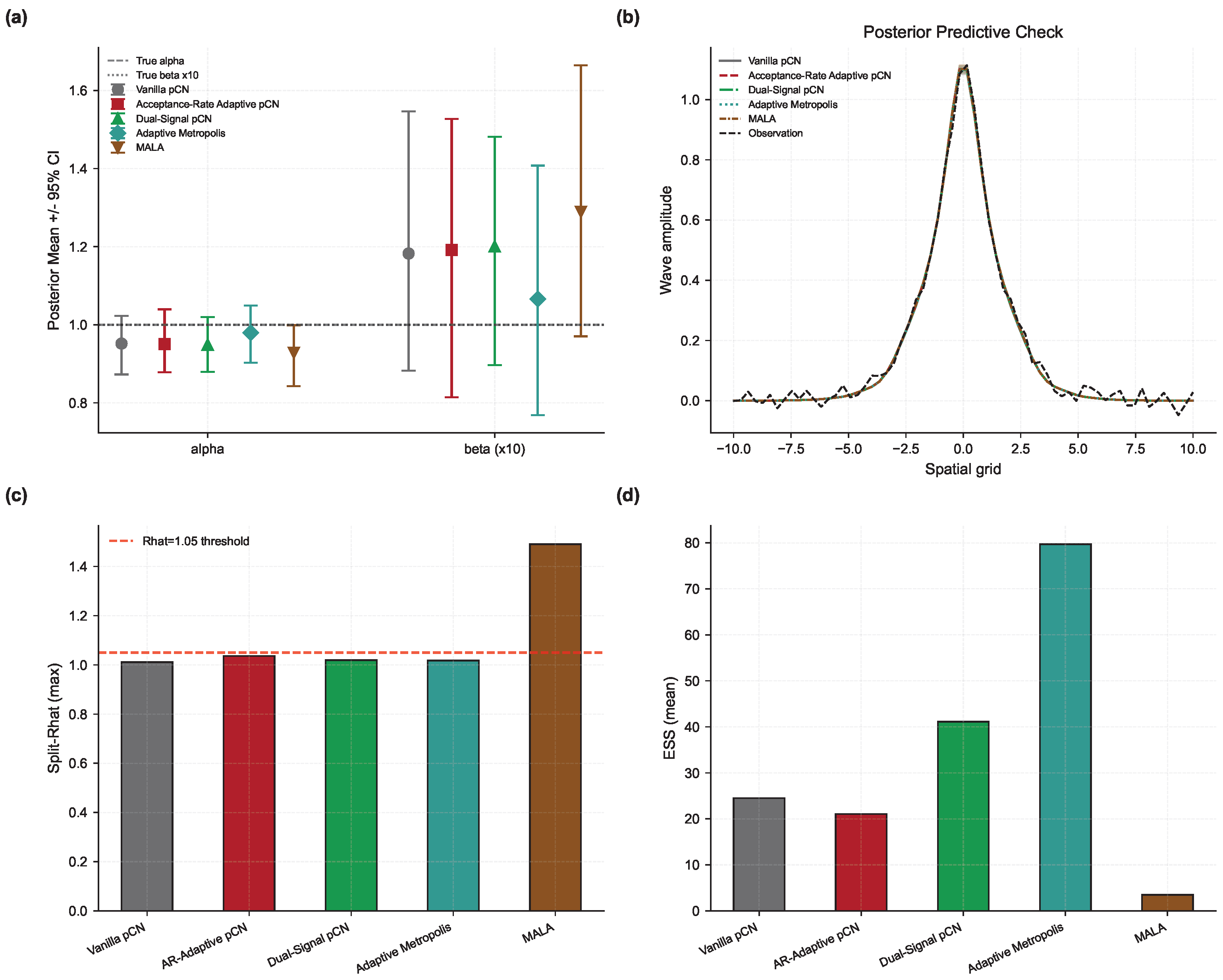
The sampling diagnostics (Figure 7) show that the AM exhibited the fastest autocorrelation decay and smoothest trace plots, followed by the three pCN variants, which showed comparable mixing behavior. The MALA’s trace plots revealed poor exploration, consistent with its low ESS and high $\widehat{R}$. The split-$\widehat{R}$ values (Figure 8, panel (c)) indicate reasonable convergence for all pCN variants and the AM ($\widehat{R}\le 1.036$), while the MALA remained far from convergence ($\widehat{R}=1.49$).

Figure 7. Sampling diagnostics for the CQNLSE inverse problem across all five methods. (a) Trace plots of $\alpha$; (b) trace plots of $\beta$; (c) autocorrelation functions for $\alpha$; (d) autocorrelation functions for $\beta$; and (e,f) posterior marginal densities. The AM showed the fastest decorrelation, while the MALA exhibited poor mixing.

Figure 8. Uncertainty quantification and posterior predictive validation for the CQNLSE inverse problem across all five methods. (a) Posterior means and 95% credible intervals for $\alpha$ and $\beta$; (b) posterior predictive bands for the terminal wave profile; (c) split-$\widehat{R}$ values; and (d) the ESS and wall-clock time.

Uncertainty quantification and posterior predictive checks (Figure 8) indicate that all methods produced credible intervals containing the true coefficients (panel (a)). The AM yielded the tightest credible intervals for both $\alpha$ and $\beta$, consistent with its superior ESS and convergence diagnostics. The posterior predictive distributions reproduce the general features of the observed wave profile (panel (b)), and panel (d) highlights the efficiency differences across methods in terms of the ESS and wall-clock time.

Overall, the CQNLSE benchmark demonstrates that the AM provided the best performance on this low-dimensional nonlinear problem, while among the pCN variants, acceptance rate adaptation yielded modest, but consistent, improvements. The MALA result should be interpreted in light of the finite-difference implementation and the limited computational budget.

4.5. Sensitivity Analysis

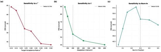
We assessed the sensitivity of the acceptance rate-adaptive pCN to hyperparameter choices by varying three key parameters: the target acceptance rate ${\alpha }^{*}$, the adaptation interval K, and the burn-in fraction. All experiments used the ill-conditioned linear-Gaussian benchmark ($d=80$, $\kappa =200$) with the acceptance rate-adaptive pCN and four chains. The results are summarized in Figure 9 and Table 6.

Figure 9. Sensitivity analysis of the acceptance rate-adaptive pCN on the ill-conditioned benchmark ($d=80$, $\kappa =200$). (a) ESS and $\widehat{R}$ versus target acceptance rate ${\alpha }^{*}$. (b) ESS and $\widehat{R}$ versus adaptation interval K. (c) ESS and $\widehat{R}$ versus burn-in fraction. The method was moderately sensitive to all three hyperparameters, with the default settings providing a robust performance.

Table 6. Sensitivity analysis of acceptance rate-adaptive pCN hyperparameters on the ill-conditioned benchmark ($d=80$, $\kappa =200$).

Parameter	Value	ESS	ESS/s	$\widehat{\mathit{R}}$
${\alpha }^{*}$	0.10	64.2	14.97	1.233
${\alpha }^{*}$	0.234 (default)	52.2	12.14	1.321
${\alpha }^{*}$	0.50	43.3	10.09	1.613
K	50	89.5	20.93	1.213
K	200 (default)	53.8	12.55	1.395
K	800	40.1	9.30	1.456
Burn-in	0.05	41.0	9.59	1.403
Burn-in	0.25	57.9	13.50	1.308
Burn-in	0.30 (default)	52.5	12.23	1.385
Burn-in	0.50	49.9	10.57	1.313

By varying the target acceptance rate ${\alpha }^{*}$ from $0.10$ to $0.50$, we observed a monotonic decrease in the ESS as ${\alpha }^{*}$ increased beyond the theoretically optimal $0.234$. The best performance occurred at ${\alpha }^{*}=0.10$ (ESS = 64.2), while the standard choice ${\alpha }^{*}=0.234$ yielded an ESS = 52.2. Higher targets (${\alpha }^{*}=0.40$–$0.50$) produced a substantially lower ESS (43–44) and degraded convergence ($\widehat{R}>1.4$). This confirms that targeting overly conservative acceptance rates leads to overly cautious proposals and a reduced exploration efficiency.

Regarding the adaptation interval, the update interval K controls how frequently the step size is adjusted. Smaller intervals ($K=50$, ESS = 89.5) allow for faster adaptation, but may introduce noise from unstable acceptance rate estimates. Larger intervals ($K=800$, ESS = 40.1) result in sluggish adaptation that fails to converge to an effective step size within the burn-in budget. The intermediate values $K=100$–200 provide a good balance, with $K=100$ achieving an ESS = 77.2.

As for the burn-in fraction, the fraction of the chain devoted to adaptation affects both the quality of the adapted step size and the number of retained samples. A very short burn-in ($5\%$, ESS = 41.0) provides insufficient adaptation time, while moderate fractions ($25\%$, ESS = 57.9) achieve near-optimal performance. Burn-in fractions above $30\%$ show diminishing returns as the reduced post-burn-in sample size begins to dominate. The default $30\%$ burn-in (ESS = 52.5) represents a conservative choice that ensures reliable adaptation across problem configurations.

The sensitivity analysis shows that the default hyperparameter settings (${\alpha }^{*}=0.234$, $K=200$, burn-in = 30%) deliver a performance close to the best observed across the tested range. The method degrades gracefully: even with suboptimal hyperparameter choices, the adaptive scheme substantially outperforms vanilla pCN (ESS = 30.5), confirming that the primary benefit of adaptation—eliminating manual step-size tuning—holds across a wide range of configurations.

4.6. Multi-Seed Uncertainty Quantification

We assessed the reproducibility by repeating the ill-conditioned benchmark ($d=80$, $\kappa =200$) with five independent random seeds per method. Table 7 reports the mean and standard deviation of key metrics across seeds.

Table 7. Multi-seed uncertainty quantification ($d=80$, $\kappa =200$, 5 seeds). Values reported as mean ± standard deviation.

Method	ESS	ESS/s	ESS/eval	$\widehat{\mathit{R}}$	AR	Errμ
Vanilla pCN	$31.0\pm 1.1$	$6.5\pm 0.2$	$0.0016$	$1.70\pm 0.12$	$0.773$	$1.53\pm 0.06$
AR-Adaptive pCN	$55.7\pm 2.2$	$12.4\pm 0.9$	$0.0028$	$1.33\pm 0.09$	$0.643$	$1.48\pm 0.04$
Dual-Signal pCN	$36.3\pm 2.6$	$6.5\pm 0.4$	$0.0018$	$1.56\pm 0.13$	$0.737$	$1.50\pm 0.03$
AM	$64.6\pm 2.6$	$12.3\pm 1.8$	$0.0032$	$1.26\pm 0.02$	$0.242$	$1.77\pm 0.06$
MALA	$59.7\pm 4.2$	$6.0\pm 0.6$	$0.0030$	$1.27\pm 0.04$	$0.408$	$1.76\pm 0.03$

The results demonstrate a low variance across seeds for all methods, with relative standard deviations in the ESS being below $10\%$ in all cases. The AR-adaptive pCN consistently achieved an approximately $1.8\times$ higher ESS than vanilla pCN across all seeds, and its $\widehat{R}$ values were significantly lower ($1.33\pm 0.09$ versus $1.70\pm 0.12$), confirming the robustness of the improvement. The AM and MALA showed competitive ESS values ($64.6$ and $59.7$, respectively), but with higher posterior mean errors, suggesting that, while these methods generate more effectively independent samples, their proposals may introduce bias in the posterior mean estimate at this sample size. The low inter-seed variance across all methods confirms that the reported performance differences are systematic rather than stochastic artifacts.

4.7. Comparison with Adaptive Metropolis and MALA

Comparing with AM and MALA clarifies the positioning of the adaptive pCN variants relative to established alternatives. The results highlight several distinctions.

In terms of the regime-dependent performance, the AM achieved the highest ESS in well-conditioned (ESS = 147.9) and low-SNR (ESS = 83.0) regimes where the posterior is relatively isotropic and the empirical covariance provides a good approximation to the posterior geometry. However, in the ill-conditioned regime, the AM’s advantage narrowed (ESS = 60.0 versus AR-adaptive pCN’s 56.4), and in the high-SNR regime, the AM underperformed (ESS = 28.5 versus AR-adaptive pCN’s 36.2), likely because the sharp posterior concentrated along a few directions makes covariance adaptation more challenging. The MALA showed a similar pattern: an excellent performance in low-SNR (ESS = 134.9), but a degraded performance in high-SNR (ESS = 28.7) and ill-conditioned settings.

Regarding the computational cost, the pCN variants had the lowest per-iteration cost, completing in $3.8$–$6.4$ s across all regimes. The AM incurred $1.5$–$2\times$ overhead from covariance matrix operations (Cholesky factorization, Welford updates), requiring $5.3$–$7.0$ s. The MALA was the most expensive, at $9.2$–$20.2$ s due to gradient computation, which, for the linear-Gaussian case, involves matrix-vector products and, for CQNLSE, requires finite-difference approximation with multiple forward model evaluations.

For the CQNLSE benchmark, the AM substantially outperformed all pCN variants (ESS = 304.5 versus 145–172), confirming that covariance adaptation is highly effective for low-dimensional problems with strong parameter coupling. The MALA mixed poorly in our finite-difference implementation (ESS = 12.9, $\widehat{R}=1.49$). The extra cost and possible inaccuracy of the finite-difference gradients may partly explain this result.

Acceptance rate-adaptive pCN is most useful when the prior is Gaussian, gradients are unavailable or expensive, and adapting a full covariance matrix is undesirable, as in moderate-dimensional problems with costly forward models. It has a low adaptation overhead and avoids manual step-size tuning. In contrast, the AM may be preferable in low-dimensional or well-conditioned problems, while the MALA can be more efficient when accurate gradients are inexpensive.

5. Conclusions

This work tackled a practical limitation of the pCN algorithm in Bayesian inverse problems—its sensitivity to manual tuning of the proposal step-size parameter $\beta$. We introduced two adaptive pCN variants (acceptance rate-adaptive and dual-signal pCN) and compared them with the vanilla pCN, adaptive Metropolis (AM), and MALA across benchmarks with dimensions of $d=10$ to 100, condition numbers of $\kappa =2$ to 200, an SNR from $-9$ dB to $+8$ dB, and a nonlinear PDE-constrained problem.

Both adaptive pCN variants preserved posterior consistency by restricting adaptation to a finite burn-in phase and freezing the step size thereafter. The retained chain is a standard time-homogeneous MH kernel, under which ergodicity and Monte Carlo consistency follow from classical Markov chain theory. A conditional spectral-gap argument characterizes the post-adaptation convergence rate.

Numerical experiments showed that different methods excel in different regimes. The acceptance rate-adaptive pCN gave the most consistent improvement over vanilla pCN across all linear-Gaussian benchmarks ($1.8\times$ ESS improvement on average in the ill-conditioned regime with a low inter-seed variance). The AM performed best on well-conditioned and low-dimensional problems, where covariance adaptation captures posterior geometry, but incurs a higher computational cost and shows diminishing returns under strong anisotropy. The MALA excelled in low-SNR regimes, but degraded in high-SNR settings and mixed poorly on the CQNLSE benchmark. The latter result may partly reflect the use of finite-difference gradients. A sensitivity analysis confirmed that the adaptive pCN is robust to hyperparameter variations, with the default settings giving a near-optimal performance across the tested range. Multi-seed experiments support the conclusion that the reported improvements on the linear-Gaussian benchmarks are systematic and reproducible.

Two limitations should be noted. First, the linear-Gaussian benchmarks were limited to $d\le 100$, which is moderate rather than truly high-dimensional by the standards of modern large-scale Bayesian inverse problems. Second, the nonlinear CQNLSE example involved only two unknown parameters and served as a proof of concept for nonlinear forward operators rather than a demonstration of high-dimensional nonlinear scalability. Extending the framework to genuinely high-dimensional nonlinear problems ($d\gg 100$) is a natural next step.

Finally, we note that the current experimental validation is limited to linear-Gaussian benchmarks and a single nonlinear PDE-constrained problem (CQNLSE). Extending the adaptive framework to additional nonlinear inverse problems—such as PDE coefficient identification, diffusion inverse problems, and tomographic reconstruction—represents an important priority for future work.

Several directions remain open. Extending the adaptive framework to high-dimensional nonlinear inverse problems with expensive PDE forward models would broaden its practical reach. Combining the step-size adaptation mechanism with geometric MCMC methods—such as Riemannian manifold Langevin or Hamiltonian Monte Carlo—could exploit local posterior geometry for additional efficiency gains. A theoretical characterization of the transient adaptation dynamics during burn-in, rather than only the post-freezing behavior, would improve the understanding of stochastic-approximation-driven MCMC. Applying the framework to real-world inverse problems in medical imaging, geoscience, and computational fluid dynamics is also a promising direction.

References

- Kaipio, J.; Somersalo, E. Statistical and Computational Inverse Problems; Springer: New York, NY, USA, 2005. [Google Scholar] [CrossRef] [Scilit]
- Gelman, A.; Carlin, J.B.; Stern, H.S.; Dunson, D.B.; Vehtari, A.; Rubin, D.B. Bayesian Data Analysis, 3rd ed.; Chapman & Hall/CRC: Boca Raton, FL, USA, 2013. [Google Scholar] [CrossRef] [Scilit]
- Arridge, S.R. Optical tomography in medical imaging. Inverse Probl. 1999, 15, R41–R93. [Google Scholar] [CrossRef] [Scilit]
- Starck, J.L.; Murtagh, F.; Fadili, J.M. Sparse Image and Signal Processing: Wavelets, Curvelets, Morphological Diversity; Cambridge University Press: Cambridge, UK, 2010. [Google Scholar] [CrossRef] [Scilit]
- Amoudruz, L.; Litvinov, S.; Papadimitriou, C.; Koumoutsakos, P. Bayesian inference for PDE-based inverse problems using the optimization of a discrete loss. Comput. Methods Appl. Mech. Eng. 2026, 455, 118903. [Google Scholar] [CrossRef] [Scilit]
- Cotter, S.L.; Roberts, G.O.; Stuart, A.M.; White, D. MCMC methods for functions: Modifying old algorithms to make them faster. Stat. Sci. 2013, 28, 424–446. [Google Scholar] [CrossRef] [Scilit]
- Neal, R.M. MCMC using Hamiltonian dynamics. In Handbook of Markov Chain Monte Carlo; Brooks, S., Gelman, A., Jones, G.L., Meng, X.L., Eds.; Chapman & Hall/CRC: Boca Raton, FL, USA, 2011; pp. 113–162. [Google Scholar] [CrossRef] [Scilit]
- Qian, J.; Liu, Y.; Yang, J.; Zhou, Q. Bayesian imaging inverse problem with SA-Roundtrip prior via HMC-pCN sampler. Comput. Stat. Data Anal. 2024, 196, 107930. [Google Scholar] [CrossRef] [Scilit]
- Ou, N.; Zhang, Z.; Lin, G. A replica exchange preconditioned Crank–Nicolson Langevin dynamic MCMC method with multi-variance strategy for Bayesian inverse problems. J. Comput. Phys. 2024, 510, 113067. [Google Scholar] [CrossRef] [Scilit]
- Carrera, B.; Papaioannou, I. Covariance-based MCMC for high-dimensional Bayesian updating with sequential Monte Carlo. Probabilistic Eng. Mech. 2024, 77, 103667. [Google Scholar] [CrossRef] [Scilit]
- Cui, T.; Martin, J.; Marzouk, Y.M.; Solonen, A.; Spantini, A. Likelihood-informed dimension reduction for nonlinear inverse problems. Inverse Probl. 2014, 30, 114015. [Google Scholar] [CrossRef] [Scilit]
- Cui, T.; Law, K.J.H.; Marzouk, Y.M. Dimension-independent likelihood-informed MCMC for large-scale inverse problems. J. Comput. Phys. 2016, 304, 109–137. [Google Scholar] [CrossRef] [Scilit]
- Beskos, A.; Girolami, M.; Lan, S.; Farrell, P.E.; Stuart, A.M. Geometric MCMC for infinite-dimensional inverse problems. J. Comput. Phys. 2017, 335, 327–351. [Google Scholar] [CrossRef] [Scilit]
- Girolami, M.; Calderhead, B. Riemann manifold Langevin and Hamiltonian Monte Carlo methods. J. R. Stat. Soc. Ser. B Stat. Methodol. 2011, 73, 123–214. [Google Scholar] [CrossRef] [Scilit]
- Parno, M.D.; Marzouk, Y.M. Transport map accelerated Markov chain Monte Carlo. SIAM/ASA J. Uncertain. Quantif. 2018, 6, 645–682. [Google Scholar] [CrossRef] [Scilit]
- Liu, M.; Grana, D.; Mosegaard, K.; Sen, M.K.; Xu, M.; Mukerji, T. Bayesian Inference for Subsurface Geophysical Inverse Problems. Rev. Geophys. 2026, 64, e2025RG000884. [Google Scholar] [CrossRef] [Scilit]
- Hoffman, M.D.; Gelman, A. The No-U-Turn sampler: Adaptively setting path lengths in Hamiltonian Monte Carlo. J. Mach. Learn. Res. 2014, 15, 1593–1623. [Google Scholar] [CrossRef] [Scilit]
- Haario, H.; Saksman, E.; Tamminen, J. An adaptive Metropolis algorithm. Bernoulli 2001, 7, 223–242. [Google Scholar] [CrossRef] [Scilit]
- Roberts, G.O.; Rosenthal, J.S. Examples of adaptive MCMC. Stat. Comput. 2009, 18, 349–367. [Google Scholar] [CrossRef] [Scilit]
- Andrieu, C.; Thoms, J. A tutorial on adaptive MCMC. Stat. Comput. 2008, 18, 343–373. [Google Scholar] [CrossRef] [Scilit]
- Andrieu, C.; Moulines, É. On the ergodicity properties of some adaptive MCMC algorithms. Ann. Appl. Probab. 2006, 16, 1462–1505. Available online: http://www.jstor.org/stable/25442804 (accessed on 15 July 2026). [CrossRef] [Scilit]
- Atchadé, Y.F.; Rosenthal, J.S. On adaptive Markov chain Monte Carlo algorithms. Bernoulli 2005, 11, 815–828. [Google Scholar] [CrossRef] [Scilit]
- Hu, Z.; Yao, Z.; Li, J. On an adaptive preconditioned Crank–Nicolson MCMC algorithm for infinite dimensional Bayesian inference. J. Comput. Phys. 2017, 332, 492–503. [Google Scholar] [CrossRef] [Scilit]
- Arabpour, A.; Moghadam, R.H.; Niri, M.E. Geophysical bayesian inverse problem solving with tuning-free adaptive MCMC sampler. Earth Sci. Inform. 2025, 18, 186. [Google Scholar] [CrossRef] [Scilit]
- Chada, N.K.; Jasra, A.; Maama, M.; Tempone, R. Unbiased parameter estimation for bayesian inverse problems. Stat. Comput. 2025, 36, 17. [Google Scholar] [CrossRef] [Scilit]
- Roberts, G.O.; Rosenthal, J.S. Optimal scaling of discrete approximations to Langevin diffusions. J. R. Stat. Soc. Ser. B Stat. Methodol. 1998, 60, 255–268. [Google Scholar] [CrossRef] [Scilit]
- Stuart, A.M. Inverse problems: A Bayesian perspective. Acta Numer. 2010, 19, 451–559. [Google Scholar] [CrossRef] [Scilit]
- Beskos, A.; Roberts, G.; Stuart, A.; Voss, J. MCMC methods for diffusion bridges. Stoch. Dyn. 2008, 8, 319–350. [Google Scholar] [CrossRef] [Scilit]
- Vehtari, A.; Gelman, A.; Simpson, D.; Carpenter, B.; Bürkner, P.C. Rank-normalization, folding, and localization: An improved for assessing convergence of MCMC. Bayesian Anal. 2021, 16, 667–718. [Google Scholar] [CrossRef] [Scilit]
Disclaimer/Publisher’s Note: The statements, opinions and data contained in all publications are solely those of the individual author(s) and contributor(s) and not of MDPI and/or the editor(s). MDPI and/or the editor(s) disclaim responsibility for any injury to people or property resulting from any ideas, methods, instructions or products referred to in the content. |
© 2026 by the authors. Licensee MDPI, Basel, Switzerland. This article is an open access article distributed under the terms and conditions of the Creative Commons Attribution (CC BY) license.