A VMD-JMD Hybrid Decomposition and CFC-FLCA Network for COVID-19 Multi-Step Epidemic Forecasting

Abstract

To address the high non-stationarity of COVID-19 pandemic time-series data and the severe error accumulation issue in long-horizon forecasting, a spatiotemporal two-branch multi-step forecasting model named CFC-FLCA is proposed. This model integrates closed-form continuous-time neural networks (CFC), a hybrid decomposition strategy combining variational mode decomposition (VMD) and jump plus AM-FM mode decomposition (JMD), and a cross-attention (CA) mechanism. First, the VMD-JMD hybrid mode decomposition method is applied to preprocess raw new case sequences. By leveraging the complementary advantages of the two decomposition algorithms, non-stationary sequences are adaptively decomposed into high-frequency noise components and low-to-mid-frequency trend-periodic components, eliminating random disturbance interference at the data source. On this basis, a time–frequency dual-branch feature extraction network is constructed. CFC provides ultra-long-range temporal dependency modeling capability; the time-domain branch adopts Legendre projection units (LPU) to extract robust temporal evolution features, while the frequency-domain branch employs frequency-enhanced units (FEU) to uncover latent periodic patterns that are difficult to capture using traditional time-domain methods. A cross-attention mechanism is introduced to dynamically learn the importance weights of time–frequency-domain features, enabling the adaptive deep integration of complementary information and effectively mitigating error accumulation in long-horizon forecasting. Multi-step forecasting experiments are conducted on real-world COVID-19 datasets from Belgium, the Czech Republic, and Ireland, with comprehensive comparisons against mainstream time series forecasting models. The experimental results demonstrate that the CFC-FLCA model outperforms all comparison models across all evaluation metrics for all prediction horizons.

1. Introduction

COVID-19 exhibits the core characteristics of a once-in-a-century pandemic pathogen. Its global spread not only directly threatens the lives and health of the entire population but has also severely disrupted the normal order of people’s work and daily lives, causing incalculable damage to global socioeconomic development [1]. Although countries have implemented targeted prevention and control measures, the spatiotemporal variability in COVID-19 incidence necessitates the formulation of regionalized public health policies, which has significantly increased the practical need for timely assessments of local epidemic trends, resource reserves, and transmission risks [2]. Accurate infectious disease forecasting is a core prerequisite for achieving scientific epidemic control and early warning, and holds critical practical significance for safeguarding public health, maintaining the stability of healthcare systems, and balancing epidemic prevention and control with socioeconomic development [3].

Since the outbreak of the COVID-19 pandemic, research on the epidemiological trends and transmission dynamics of the novel coronavirus, both domestically and internationally, has primarily relied on two core analytical methods: mathematical modeling-based prediction methods and artificial intelligence (AI)-based prediction methods [4]. Mathematical model-based forecasting methods include transmission dynamics models and time series models. Transmission dynamics models can quantitatively analyze the mechanisms of infectious disease transmission and predict epidemic trends [5], while time series analysis relies on statistical patterns in time-series data to forecast future values [6]. The former heavily relies on predefined assumptions regarding transmission mechanisms and lacks adaptability to dynamic real-world scenarios such as viral mutations and adjustments to prevention and control policies. The latter struggles to capture the nonlinear and abrupt characteristics of epidemic development, leading to a significant decline in long-term prediction accuracy. Continuous breakthroughs in artificial intelligence technology have enabled deep learning models—which possess superior nonlinear fitting capabilities and multi-level feature abstraction advantages—to gradually become the mainstream method in the field of disease prediction. Reference [7] employs autoregressive moving average (ARMA) models and vector autoregressive models to analyze the COVID-19 infection processes in Italy and Spain and to predict the characteristics and dynamics of the epidemic’s spread. Reference [8] constructs a machine learning-based framework for COVID-19 trend prediction and analysis to forecast the dynamic evolution and future trends of the pandemic. Reference [9] proposed a COVID-19 prediction method based on a multiple linear regression model to forecast the number of new active cases during the pandemic. While the aforementioned traditional machine learning models struggle to extract deep-level features from the data, deep learning models, leveraging the automatic feature learning capabilities of neural networks, demonstrate superior generalization and predictive performance.

Reference [10] proposed a combined prediction model based on k-means clustering and LSTM neural networks to forecast the number of confirmed COVID-19 cases. Reference [11] employed three types of deep learning models—long short-term memory network (LSTM), gated recurrent unit (GRU), and bidirectional long short-term memory (Bi-LSTM)—to achieve high-precision predictions of COVID-19 epidemic trends, leveraging their strong fitting capabilities for nonlinear time-series data and their ability to capture long-term temporal dependencies. Reference [12] proposed a transfer learning prediction model based on LSTM networks. Leveraging its core advantage of addressing the challenges of insufficient fitting and poor generalization in small-sample data during the early stages of the pandemic, this model was used for the precise prediction of confirmed COVID-19 cases and deaths. Reference [13] proposed a data-driven hybrid ensemble model based on multiple neural networks and reinforcement learning, leveraging the strong robustness of complementary multi-model approaches and the high-precision prediction capabilities of reinforcement learning’s adaptive optimization. Reference [14] proposed a hybrid prediction model integrating multi-head self-attention mechanisms with a Bi-LSTM network. Leveraging its comprehensive capture of bidirectional temporal features and global modeling of multidimensional information, this model was applied to high-precision long-term predictions of epidemic transmission trends and infection scales. Reference [15] constructed a hybrid deep learning model integrating convolutional neural network (CNN) and CFC. Leveraging CFC’s efficient modeling of sequence features and its lightweight advantages, this model is used for the benign, malignant classification of skin cancer lesions and disease risk prediction. Reference [16] proposed an ODE-LSTM model integrating liquid time-constant (LTC) and LSTM. Leveraging its strong modeling ability for the continuous dynamic evolution of epidemic time-series data and its adaptability to non-uniformly sampled data, this model is used for the precise prediction of new confirmed cases. However, the aforementioned methods directly use raw case time series as a single input source, failing to effectively decompose the multiscale fluctuation characteristics within the signal.

Reference [17] developed a CEEMDAN-R-ILSTM-Elman ensemble deep learning prediction model. By leveraging the advantages of complete ensemble empirical mode decomposition with adaptive noise (CEEMDAN) in smoothing nonlinear, non-stationary epidemic data, the model achieved high-precision predictions of epidemic trends in BRICS countries. Reference [18] proposed a hybrid forecasting model based on ensemble empirical mode decomposition (EEMD) and LSTM neural networks. Leveraging its advantages in multiscale feature decomposition and the nonlinear fitting of pandemic time-series data, this model was used for the precise forecasting of confirmed COVID-19 cases. Reference [19] leveraged the advantages of sequential variational mode decomposition (SVMD) in adaptively smoothing epidemic data and removing noise to achieve high-precision short-term forecasts of daily new confirmed cases and deaths. The aforementioned studies primarily employed single decomposition methods, which have certain limitations in feature extraction for complex signals. These methods struggle to fully capture multiscale information, resulting in insufficient feature representational capacity.

To address the aforementioned limitations, this study conducts the following research:

(1) The VMD-JMD hybrid modal decomposition algorithm is applied to process non-stationary infectious disease time-series data. Through multi-scale decomposition, the trend, periodic and disturbance components embedded in the raw sequence are decoupled, which effectively mitigates the adverse effects of data non-stationarity and stochastic noise, thus providing high-quality input features for subsequent prediction modeling.

(2) A novel deep learning prediction model named CFC-FLCA is proposed. The CFC backbone encodes long-range temporal dependencies of the input features; the LPU module and FEU module extract time-domain and frequency-domain features, respectively; and a cross-attention mechanism is introduced to realize adaptive multi-source feature fusion, fully capturing the coupling correlations between epidemic evolution patterns and external influencing factors.

(3) Extensive comparative experiments are carried out on public benchmark datasets, and the effectiveness of the proposed method and its functional modules are comprehensively verified via mainstream evaluation metrics.

(4) Compared with existing modal decomposition-based prediction methods relying on single decomposition strategies and single-domain feature modeling, the proposed CFC-FLCA exploits the complementary strengths of dual decomposition algorithms and achieves deep fusion of time–frequency dual-branch features. It improves decomposition quality at the data level and strengthens multi-scale temporal pattern mining at the algorithm level, yielding higher prediction accuracy and robustness for complex epidemic time series.

2. Data Preprocessing

2.1. Introduction to the Dataset

The multivariate time-series dataset adopted in this study is the publicly available integrated resource hosted on Zenodo [20]. (https://zenodo.org/records/10203446, accessed on 17 January 2026.) This composite dataset systematically aggregates multi-dimensional open-access variables covering European Union nations, with raw data retrieved from several authoritative open repositories: COVID-19 epidemiological metrics from the Our World in Data open repository, human mobility records provided by Google, meteorological indicators supplied by the Copernicus Climate Change Service (C3S), alongside social, demographic and economic statistics sourced from Eurostat and the United Nations Development Programme. Where raw records permit, all variables are unified into daily, weekly, monthly and annual time series, which enables both cross-country and in-country comparative epidemic and socioeconomic analysis. The dataset includes the following metrics: total cases, new cases, total deaths, new deaths, total tests, new tests, positive rate, stringency index, total vaccinations, people vaccinated, people fully vaccinated, new vaccinations, total boosters, retail recreation, grocery pharmacy, parks, transit stations, workplaces, and residential.

This study selected Ireland as the target region for analysis. The choice covers a period of 860 days, from 15 February 2020 to 23 June 2022. Novel coronavirus variants keep mutating with rising transmission speed, while many countries reduced the frequency of pandemic data-reporting, generating fragmented time-series data. Official COVID-19 records are from 15 February 2020 to 23 June 2022, without long-term reporting pauses or massive missing values, constructing a complete long epidemic sequence. Over this period, Ireland witnessed successive outbreaks of multiple virus variants and gradual adjustments of public health policies, which produce strong non-stationary fluctuations and external disturbances in case data. Such data features perfectly match the test requirements of our time–frequency fusion forecasting model, enabling a comprehensive evaluation of the model’s stability and prediction performance under complex real-world epidemic conditions.

2.2. Correlation Analysis

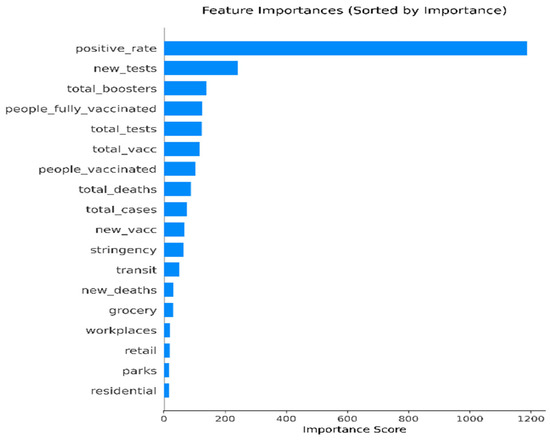
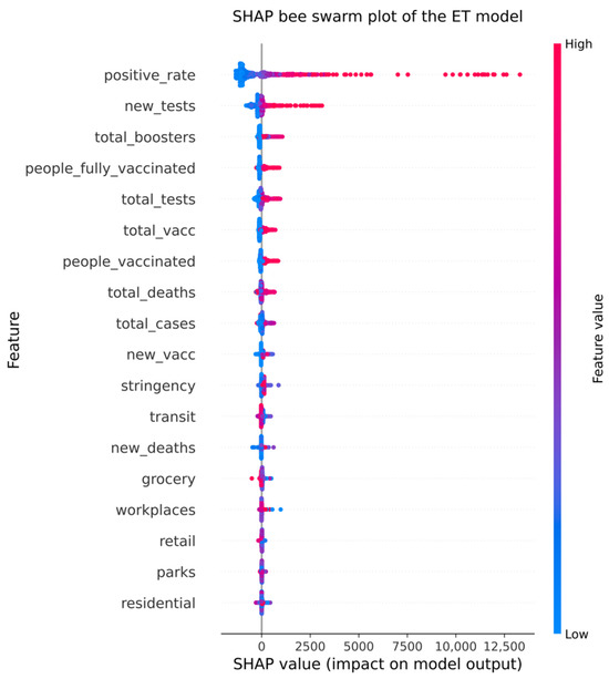
This study uses Pearson’s correlation coefficient to measure the strength of the linear relationship between daily new confirmed cases and various external factors. Extremely Randomized Trees (ET) quantify the association between each factor and the daily number of new confirmed cases, while shapley additive explanations (SHAP) scores reflect the feature importance of each factor in the model [21]. By combining these three approaches, the correlation and actual influence of each factor on new confirmed cases are comprehensively assessed, thereby providing a basis for variable selection in disease prediction models. The results of this analysis are presented in Table 1 and Figure 1. The Pearson correlation coefficients between the two datasets and are respectively expressed as

$$r_{xy}={\displaystyle \frac{{\displaystyle \sum _{i=1}^n(x_i-\overline{x})(y_i-\overline{y})}}{\sqrt{{\displaystyle \sum _{i=1}^n{(x_i-\overline{x})}^2{\displaystyle \sum _{i=1}^n{(y_i-\overline{y})}^2}}}}}$$

(1)

where $r_{xy}$ denotes the Pearson correlation coefficient between variables x and y, n is the total number of sample points in the time series, $\overline{x}$ and $\overline{y}$ are the means of x and y over all samples, $x_i$ and $y_i$ represent the values of the sample of variables x and y, respectively.

Table 1. Correlation Analysis Between Daily New Cases and External Factors.

Feature	Pearson	ET	SHAP
Total cases	0.398	0.031	74.875
Total deaths	0.393	0.036	88.072
New deaths	0.110	0.006	30.269
Total tests	0.483	0.046	123.797
New tests	0.604	0.149	242.727
Positive rate	0.780	0.501	1187.921
Stringency index	−0.248	0.008	64.820
Total vaccinations	0.500	0.030	117.214
People vaccinated	0.459	0.040	103.276
People fully vaccinated	0.483	0.040	125.542
New vaccinations	0.175	0.021	66.158
Total boosters	0.477	0.046	138.951
Retail recreation	0.167	0.006	18.633
Grocery pharmacy	0.062	0.005	29.731
Parks	−0.028	0.006	18.421
Transit stations	−0.050	0.016	51.253
Workplaces	0.067	0.006	19.631
Residential	−0.066	0.007	18.099

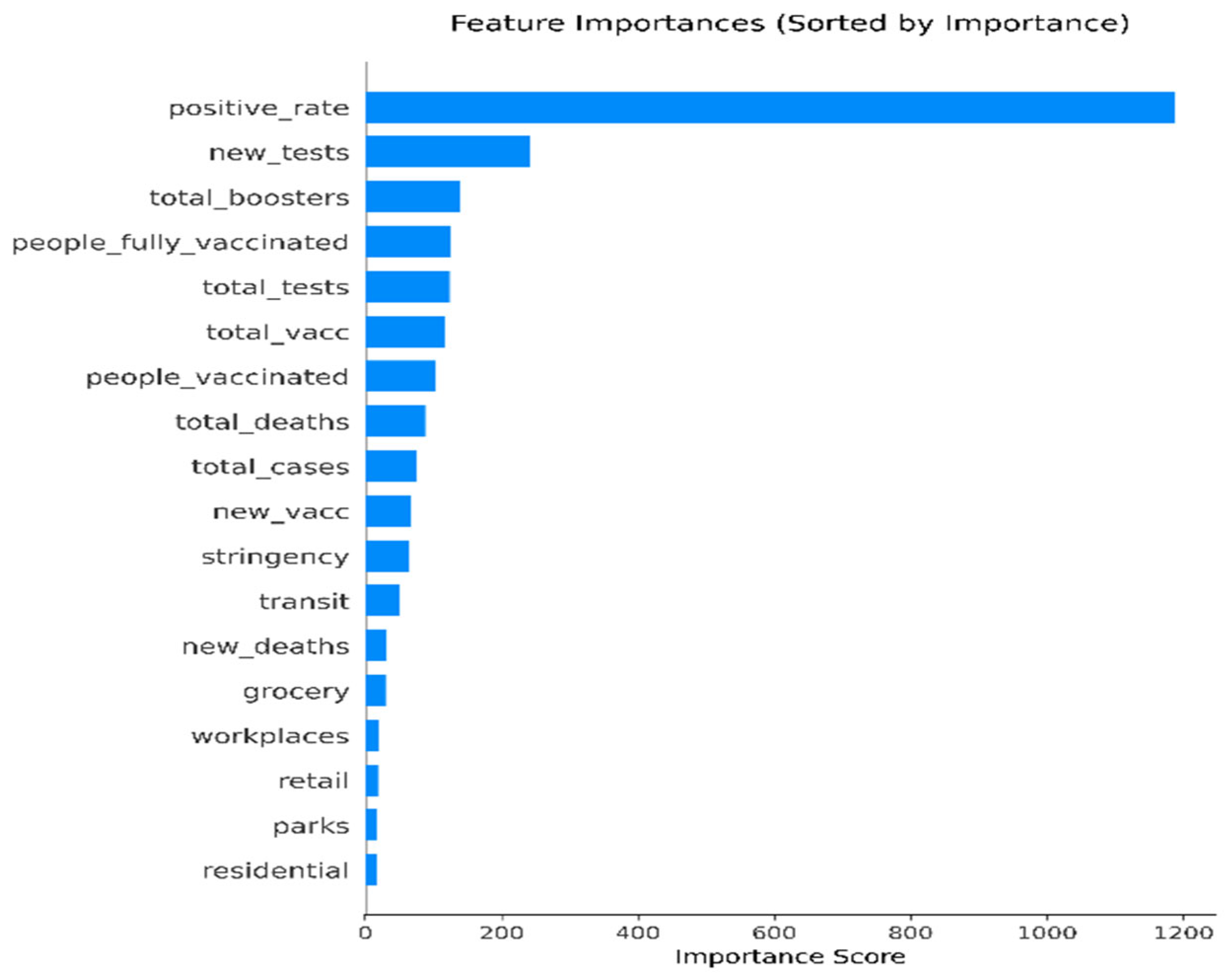
Figure 1. Results of the ET analysis for the relevant variables.

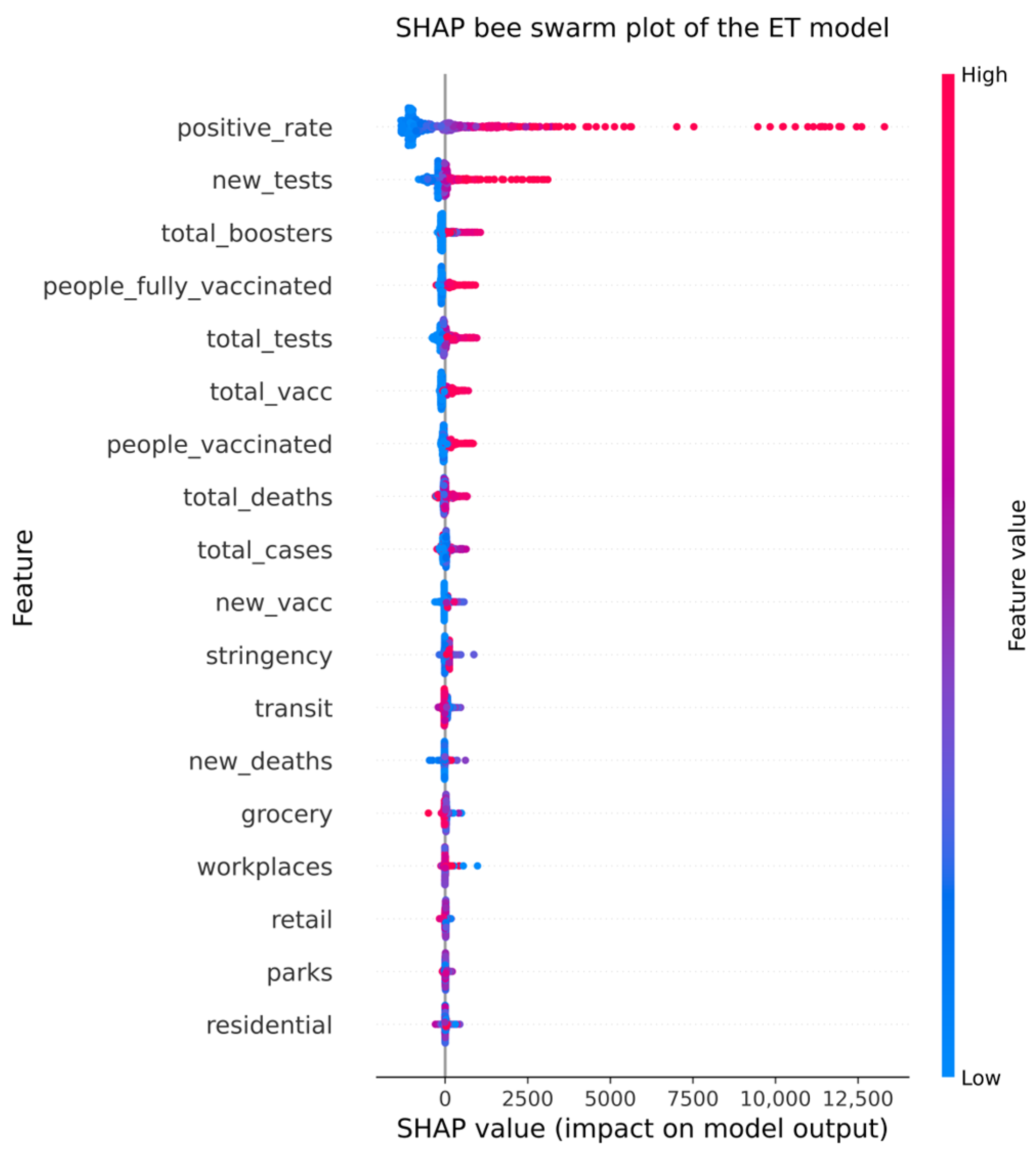
As shown in Table 1, the Pearson correlation coefficients between the nine variables and the new cases were greater than 0.2, indicating a significant linear relationship. Among these, the positivity rate and the new tests showed a strong positive correlation with the new cases, while variables such as the total vaccinations, the total tests, and the number of people fully vaccinated showed a moderate positive correlation. The correlation coefficients for new deaths, new vaccinations, and indicators of population activity such as retail recreation and transit stations were all less than 0.2, indicating an extremely weak linear relationship; these variables were therefore preliminarily excluded. As shown in Figure 1, the results of the ET model’s feature importance analysis align closely with the conclusions of the Pearson correlation analysis; variables with high correlation coefficients also consistently rank at the top in the ET importance rankings. The ET scores for positivity rate and new testing volume ranked first and second among all variables, respectively. Core variables such as booster dose volume and total testing volume also ranked highly in ET scores, confirming that these variables provide effective information gain for nonlinear prediction models and serve as the core support for model predictions. The SHAP analysis in Figure 2 further validated the robustness of feature importance and simultaneously addressed the black box issue of tree-based models. The global importance ranking is fully consistent with the results of the first two analyses and clarifies the direction of feature effects: high values for the positivity rate, testing volume, and vaccination indicators all correspond to positive SHAP contributions. That is, an increase in these indicators drives up the predicted number of new cases, which is fully consistent with the epidemiological logic of infectious diseases and provides an interpretable scientific basis for feature selection.

Figure 2. Results of the SHAP analysis for the relevant variables.

Based on this, this study ultimately identified the positivity rate, new tests, people vaccinated, total boosters, number of people fully vaccinated, total tests, total vaccinations, total cases, and total deaths as core predictive factors. This multidimensional selection strategy avoids the selection bias associated with single indicators and aligns with the characteristics of the ET model. While streamlining the feature dimensions and reducing the risk of overfitting, it balances the model’s predictive performance with interpretability.

2.3. Mixed Decomposition

JMD is a signal decomposition method based on a variational optimization framework that jointly extracts AM-FM narrowband oscillatory components and broadband jump components from non-stationary signals. By designing a joint optimization objective function and iteratively solving it using the Alternating Direction Method of Multipliers (ADMM), this method overcomes the limitations of traditional methods in handling mixed jump–oscillatory signals [22].

VMD is a signal decomposition method based on variational optimization. By constructing a constrained variational model, it decomposes a signal into multiple modal components with sparse frequency bands [23].

The time series of new cases exhibits typical characteristics of strong nonlinearity, non-stationarity, and multi-scale fluctuation coupling. The series simultaneously incorporates long-term epidemic trends, medium-term cyclical fluctuations, and short-term random disturbances caused by sudden factors. Direct modeling of the raw series is prone to noise interference and struggles to balance the accuracy of trend fitting and fluctuation capture. Single-modal decomposition methods generally suffer from inherent limitations such as mode aliasing, modal component bias, and loss of effective features, making it impossible to fully decouple the multiscale characteristics of the time series. To address this, this paper constructs a hybrid modal decomposition framework combining JMD and VMD to perform full-scale time–frequency decoupling on the raw time series of new confirmed cases, thereby overcoming the performance bottlenecks of single-modal decomposition methods.

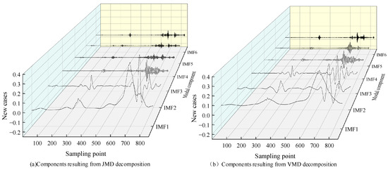
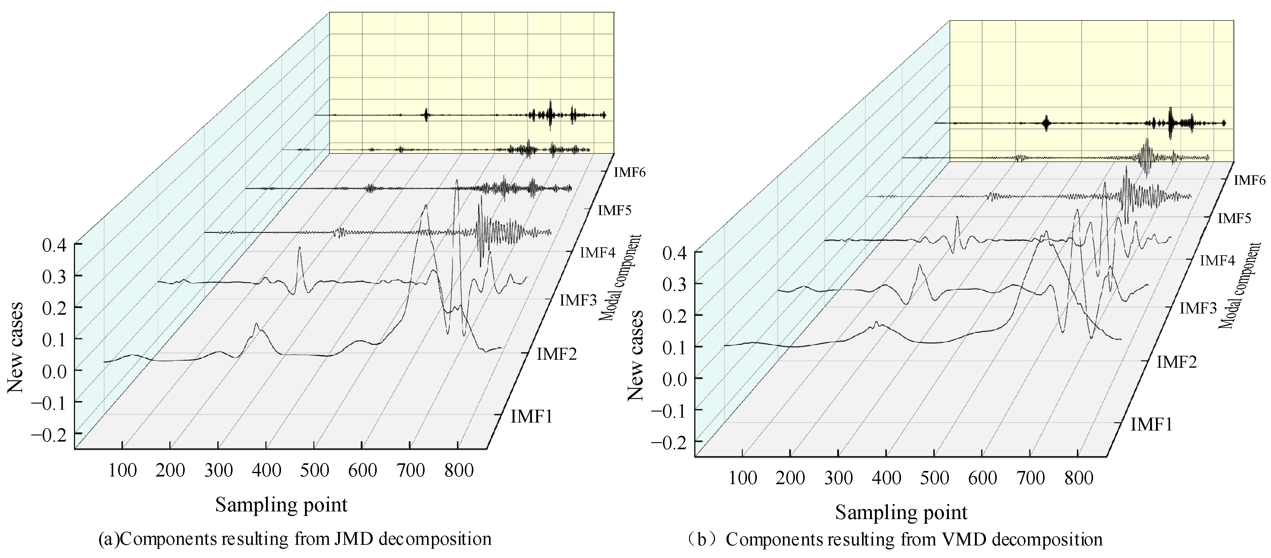
Figure 3 illustrates the component decoupling performance of different decomposition methods on the sequence of new confirmed cases. JMD decompose the original time series into six modal components across different time scales. While stripping away random noise from the sequence, it fully preserves the trend evolution characteristics and nonlinear correlation patterns of different epidemic phases, significantly reducing the difficulty of feature learning for subsequent models and laying the foundation for improved prediction accuracy and robustness. VMD decomposes the original time series into six eigenmodes, complementing JMD’s time-domain decomposition logic. Inputting the sequences obtained from JMD and VMD into deep learning prediction models enables both the collaborative exploration of detailed correlations in high-frequency fluctuations and the precise capture of long-term evolutionary trends in low-frequency components, providing comprehensive, multi-scale feature support for the accurate prediction of new confirmed cases in complex epidemic environments.

Figure 3. New cases’ decomposition results.

2.4. Dual-Branch Input Matrix Configuration

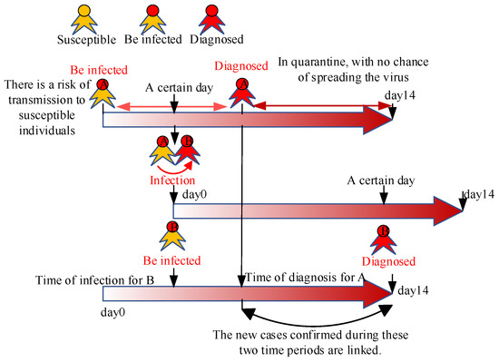
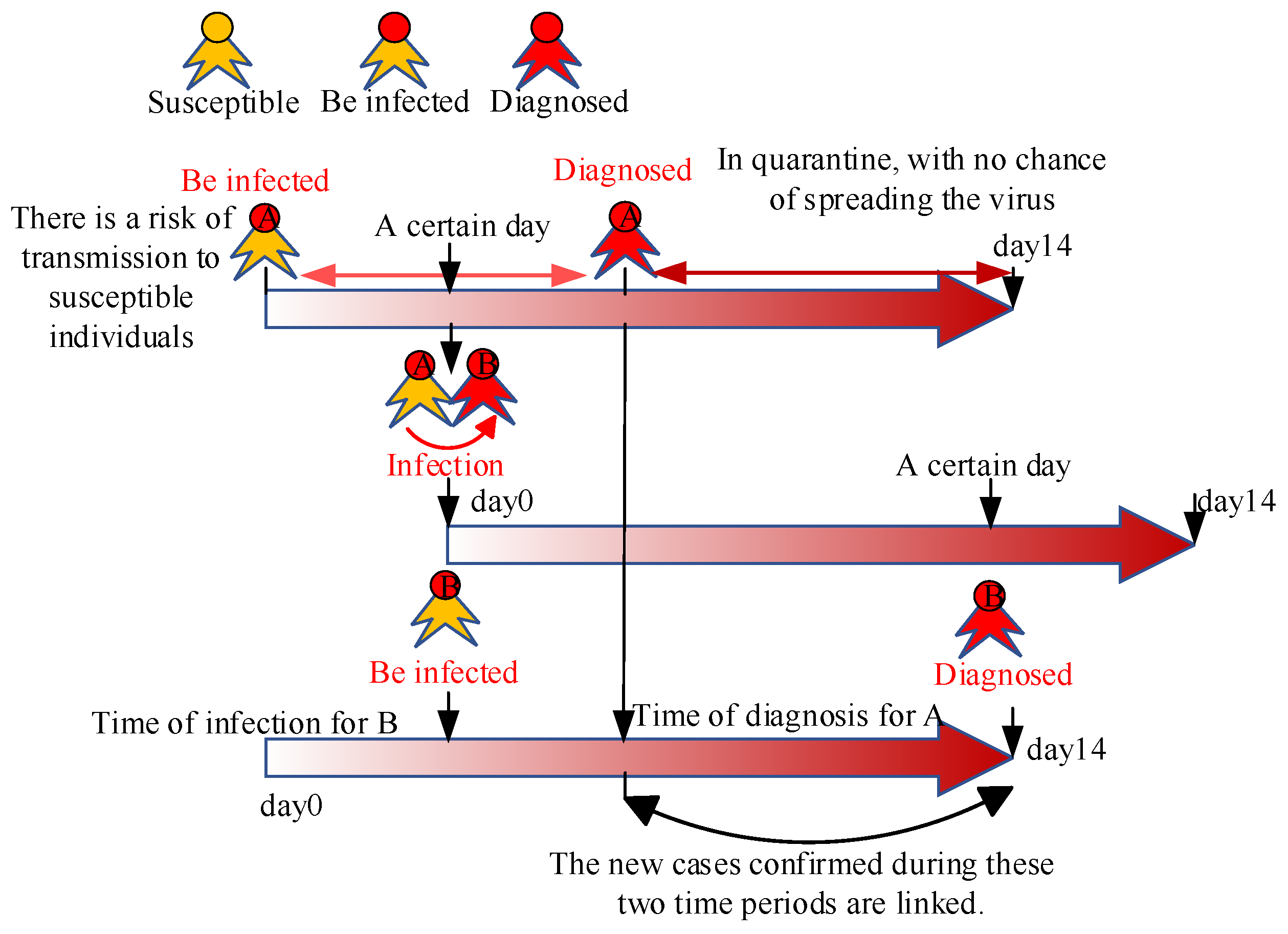
Epidemiological studies have confirmed that the implemented epidemic prevention and control measures had a significant suppressing effect on the transmission of COVID-19 approximately two weeks after their implementation. This phenomenon is highly consistent with the basic transmission dynamics of the virus: the vast majority of infected individuals develop clinical symptoms and are diagnosed within 14 days of exposure, and even if they are not promptly tested and diagnosed, they remain infectious throughout the entire incubation period [24]. The transmission timeline shown in Figure 4 further reveals that expanding the coverage of nucleic acid testing and strengthening the management of close contacts can effectively shorten an individual’s actual infectious period. Yellow icons represent susceptible individuals, red icons represent infected patients. Capital letters A and B denote two typical individual cases used to illustrate infection transmission logic. Horizontal gradient red arrows represent the 14-day infectious time window of each infected person; bidirectional horizontal arrows mark the time interval between infection onset and diagnosis; curved arrows indicate transmission links between susceptible and infected persons; the bottom curved black arrow reflects the correlation between newly confirmed cases in two distinct 14-day time windows.

Figure 4. Timeline of the spread.

Comprehensive epidemiological data indicate that the infectious period for COVID-19 patients typically does not exceed 14 days, meaning that the sources of infection for new confirmed cases reported at any given time almost exclusively originate from individuals infected within the past 14 days. Based on these core epidemiological principles, this study established a research framework that uses daily new confirmed cases and related characteristic variables from the past 14 days as model inputs to predict the number of new cases over the next 1–3 days.

The proposed model adopts a dual-branch input structure to separately model the intrinsic fluctuation patterns of the epidemic sequence and the influence of external associated factors, with strict temporal alignment between the two branches.

The new case feature matrix ${\mathit{F}}_{\mathrm{N}}\in {ℝ}^{T\times 12}$ is constructed by concatenating 12 intrinsic mode functions generated from the raw new case sequence via VMD-JMD hybrid decomposition, where T denotes the total length of the time series. The correlation variable feature matrix ${\mathit{F}}_{\mathrm{V}}\in {ℝ}^{T\times 9}$ is formed by aggregating nine external factors screened by Pearson correlation analysis, and each time step of F_V is strictly aligned with the corresponding timestamp of F_N.

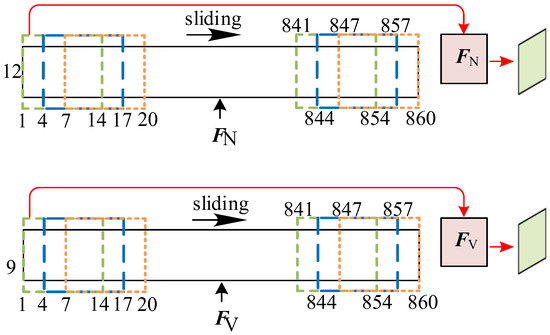
All input samples are generated via a fixed-size sliding window strategy with an input window length $l=14$ and prediction horizons of one, two, and three steps. Taking the three-step forecasting task as an example:

(1) For the new case branch, a continuous time window covering 14 consecutive time steps is intercepted from F_N to form a 14 × 12 input feature block;

(2) For the correlation variable branch, a time window with exactly the same start and end timestamps is intercepted from F_V to form a 14 × 9 input feature block, ensuring complete temporal consistency between the two branches;

(3) The ground-truth labels corresponding to the input window are the actual new case counts of the first, second, and third time steps immediately after the window.

For forecasting tasks with different step sizes, only the length of the label sequence needs to be adjusted, while the input window length, data preprocessing workflow, and dual-branch construction logic remain completely unchanged. This unified construction framework ensures the consistency and reusability of the overall method across different prediction scenarios.

Figure 5 illustrates the process of constructing time-aligned sliding windows for a dual-branch input matrix in a three-step prediction task. The upper and lower subfigures correspond to the new case feature matrix F_N and the relevant variable feature matrix F_V, respectively, with their timestamps fully synchronized. The green, blue, and orange dashed rectangles represent three different local sampling windows used for segment extraction; these two sets of colored dashed boxes show typical starting and ending positions of the sliding windows along the time series. The black right-pointing arrows indicate the synchronized left-to-right sliding direction of the windows on both branches; the vertical black upward arrows represent the types of the two matrices, respectively; and the closed red curved arrows depict the process of extracting windowed segments to generate the final feature matrix. Upon completion of the entire sliding pass, all overlapping input samples are merged, which intuitively demonstrates the overlapping sampling mechanism adopted for time-series data.

Figure 5. Constructing a double-branch input matrix.

3. Deep Learning Models with Dual-Branch Inputs

This chapter elaborates on the architecture and core components of the proposed CFC-FLCA dual-branch forecasting model. Built on the VMD-JMD hybrid decomposition preprocessing scheme, the model adopts a time–frequency dual-branch structure to capture both long-term temporal evolution patterns and latent periodic features. The subsequent subsections sequentially introduce the CFC backbone, FEU module, LPU module, cross-attention fusion mechanism, overall model structure, and the evaluation metrics used in this work.

3.1. CFC Module

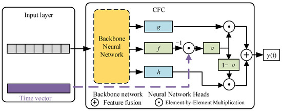
CFC are a novel type of liquid neural network proposed by Ramin M. Hasani et al. [25]. The core idea is to use continuous-time differential equations to describe the dynamic changes in neuron states in response to inputs, while allowing the time constant to adaptively adjust with the input, thereby making it a continuous-time model. The CFC module structure is shown in Figure 6. CFC is an improvement upon LTC networks, replacing the ODE solver in LTC networks with a closed-form approximation. This approach maintains accuracy while circumventing the massive computational overhead required for solving ordinary differential equations, resulting in significantly improved inference and training speeds.

Figure 6. Closed-form continuous-depth neural structure.

3.2. FEU Module

The frequency-domain enhancement unit addresses the core challenges faced by traditional time-domain deep learning models in long-term time series forecasting, including susceptibility to high-frequency noise, insufficient ability to capture long-term trends, and poor generalization performance. Taking time-series features as input, this module first maps the time-domain signal to the frequency-domain space using a real-valued Fast Fourier Transform (rFFT), leveraging the conjugate symmetry of the real-valued Fourier transform to reduce computational redundancy [26]. A low-frequency mode selection strategy is employed to identify the top k low-frequency components that are strongly correlated with the long-term evolution of the sequence, thereby filtering out high-frequency random noise with no predictive value at its source. Finally, the real and imaginary parts of the filtered frequency-domain features are separated and concatenated; after linear projection and layer normalization, high-robustness frequency-domain features of a fixed dimension are output. In disease time-series forecasting scenarios, such as the prediction of new cases, this module effectively eliminates high-frequency disturbances—including reporting delays during holidays, back-reported cases, localized cluster-induced fluctuations, and statistical sampling errors—while accurately encoding core predictive information such as the seasonal cycles, medium- to long-term growth, and decline trends of disease epidemics. This makes it well-suited for the medium- to long-term trend forecasting needs in the public health sector.

3.3. LPU Module

The mathematical foundation of the Legendre projection unit stems from the LegT orthogonal projection operator within the HiPPO (High-order Polynomial Projection Operators) framework. It is designed to address the core challenges faced by traditional time-domain deep learning models in long-term time series forecasting, including insufficient capture of long-range dependencies, high risk of gradient vanishing, and poor robustness in fitting non-stationary time series features [27]. This module takes time-series features as input and performs redundancy-free, multi-scale feature extraction in the time dimension based on the Legendre orthogonal polynomial basis. It utilizes a predefined matrix with no training parameters, uniquely determined by the orthogonality and recursive relationships of Legendre polynomials. Finally, after linear projection and layer normalization, the projected multi-scale coefficients are output as highly robust time-series features of a fixed dimension. In disease time-series forecasting scenarios, such as the prediction of new infectious disease cases, this module can accurately capture the multiscale evolutionary patterns of disease outbreaks and the long-term lagged correlations with exogenous drivers. It exhibits strong resistance to interference from sudden fluctuations in non-stationary epidemic data, significantly improving the accuracy and interpretability of medium- to long-term disease trend forecasts, thereby meeting the needs for decision-making support in public health prevention and control.

3.4. Cross-Attention Module

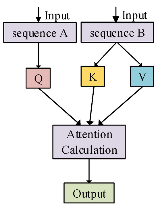
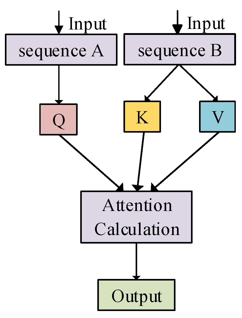
Unlike self-attention, the cross-attention mechanism models dynamic interactions across feature spaces. It addresses the core challenges of traditional linear fusion methods—namely, their inability to model nonlinear dynamic relationships between heterogeneous features and to adaptively quantify the contribution weights of different features to the prediction target. In multi-branch feature fusion scenarios, it demonstrates exceptional modeling capabilities and interpretability. This module achieves cross-branch feature association modeling by mapping the query vector (Q), key vector (K), and value vector (V) to two distinct feature spaces. Its structure is shown in Figure 7. Unlike the homogeneous design of self-attention, where Q, K, and V originate from the same feature branch, in cross-attention, Q comes from one feature branch while K and V come from another.

Figure 7. Structure of the Cross-Attention Module.

3.5. Model Structure

To address the core challenges commonly associated with new case time-series data, including strong non-stationarity, reporting delays, significant noise interference from sudden clustered fluctuations, and the limitations of traditional deep learning models in capturing long-range temporal dependencies, poor adaptability to irregularly sampled data, and weak robustness in medium- to long-term forecasting, a CFC-FLCA forecasting model is proposed for precise feature extraction and the effective integration of new case data and strongly correlated external factor data.

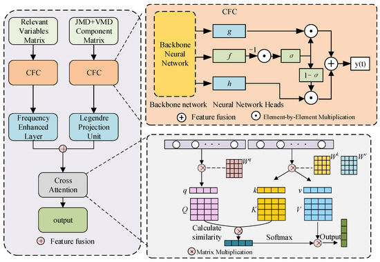
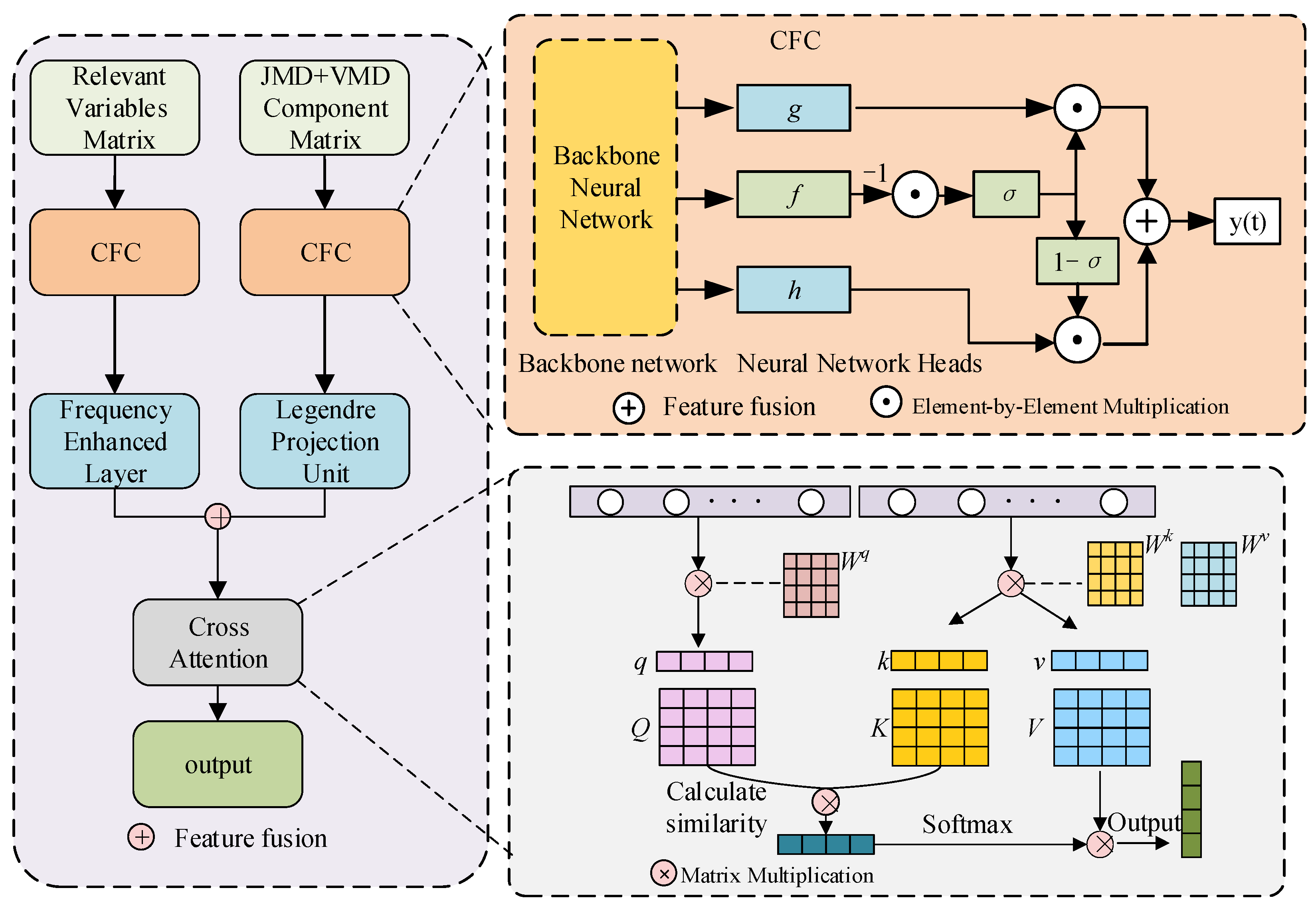
As shown in Figure 8, this model adopts a dual-branch parallel input architecture. Firstly, the CFC component performs unified modeling of the continuous-time dimension of the time series. By leveraging closed-form analytical solutions based on neural differential equations, the CFC avoids the inherent shortcomings of traditional continuous-time models, such as low computational efficiency and training instability caused by reliance on numerical integration.

Figure 8. Structure of the CFC-FLCA model.

Secondly, the two branches are fed into the FEU and LPU, respectively, to perform a targeted encoding of heterogeneous features: the branch containing the new case sequences resulting from the JMD and VMD mixed decomposition passes through the FEU, which employs real-valued fast Fourier transform and low-frequency mode selection strategies to filter out residual high-frequency reporting noise and sudden clustering fluctuations in the sequences, thereby accurately encoding the endogenous epidemic cycles and medium- to long-term evolutionary trends of the new case sequences. The branch containing highly correlated external factor data passes through the LPU, which leverages the global projection characteristics of the Legendre orthogonal polynomial basis to achieve redundancy-free, multi-scale feature extraction of exogenous driving factors, effectively capturing the long-lag correlation between external influencing factors and the sequence of new cases.

Finally, through a cross-attention mechanism, the time–frequency-domain heterogeneous features from the dual branches undergo adaptive weighting and nonlinear deep interaction, overcoming the limitation of traditional linear fusion that can only achieve static feature superposition. This mechanism adaptively quantifies the contribution weights of endogenous trend features and exogenous driving features to the prediction target, suppressing redundant interference while enhancing core effective signals. The fused features undergo dimension mapping via a fully connected layer, outputting the predicted number of new cases for the target time period.

3.6. Model Evaluation Metrics

To systematically evaluate the performance of the predictive models, this study employed four commonly used error metrics: mean absolute error (MAE), mean absolute percentage error (MAPE), root mean square error (RMSE), and coefficient of determination (R²). The formulas for calculating these error metrics are as follows:

$$E_{\mathrm{MAE}}={\displaystyle \frac{1}{m}}{\displaystyle \sum _{i=1}^m|P_i-{\widehat{P}}_i|}$$

(2)

$$E_{\mathrm{MAPE}}={\displaystyle \frac{1}{m}}{\displaystyle \sum _{i=1}^m\left|\frac{P_i-{\widehat{P}}_i}{P_i}\right|}$$

(3)

$$E_{\mathrm{RMSE}}=\sqrt{{\displaystyle \frac{1}{m}}{\displaystyle \sum _{i=1}^m{(P_i-{\widehat{P}}_i)}^2}}$$

(4)

$$R^2=1-{\displaystyle \frac{{\displaystyle \sum _{i=1}^m{(P_i-{\widehat{P}}_i)}^2}}{{\displaystyle \sum _{i=1}^m{(P_i-\overline{P})}^2}}}$$

(5)

where m is the total number of samples in the test set, $P_i$ is the actual number of new cases, ${\widehat{P}}_i$ is the number of new cases predicted by the model, and $\overline{P}$ is the arithmetic mean of the actual new case values in the test set. E_MAE, E_MAPE and E_RMSE measure the deviation between predicted and actual values from absolute error, relative error and squared error perspectives, respectively; smaller values indicate higher prediction accuracy; R² reflects the proportion of data variance explained by the model, ranging from 0 to 1, where a value closer to 1 indicates a better fitting effect of the model.

4. Experimental Procedure and Framework

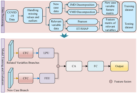
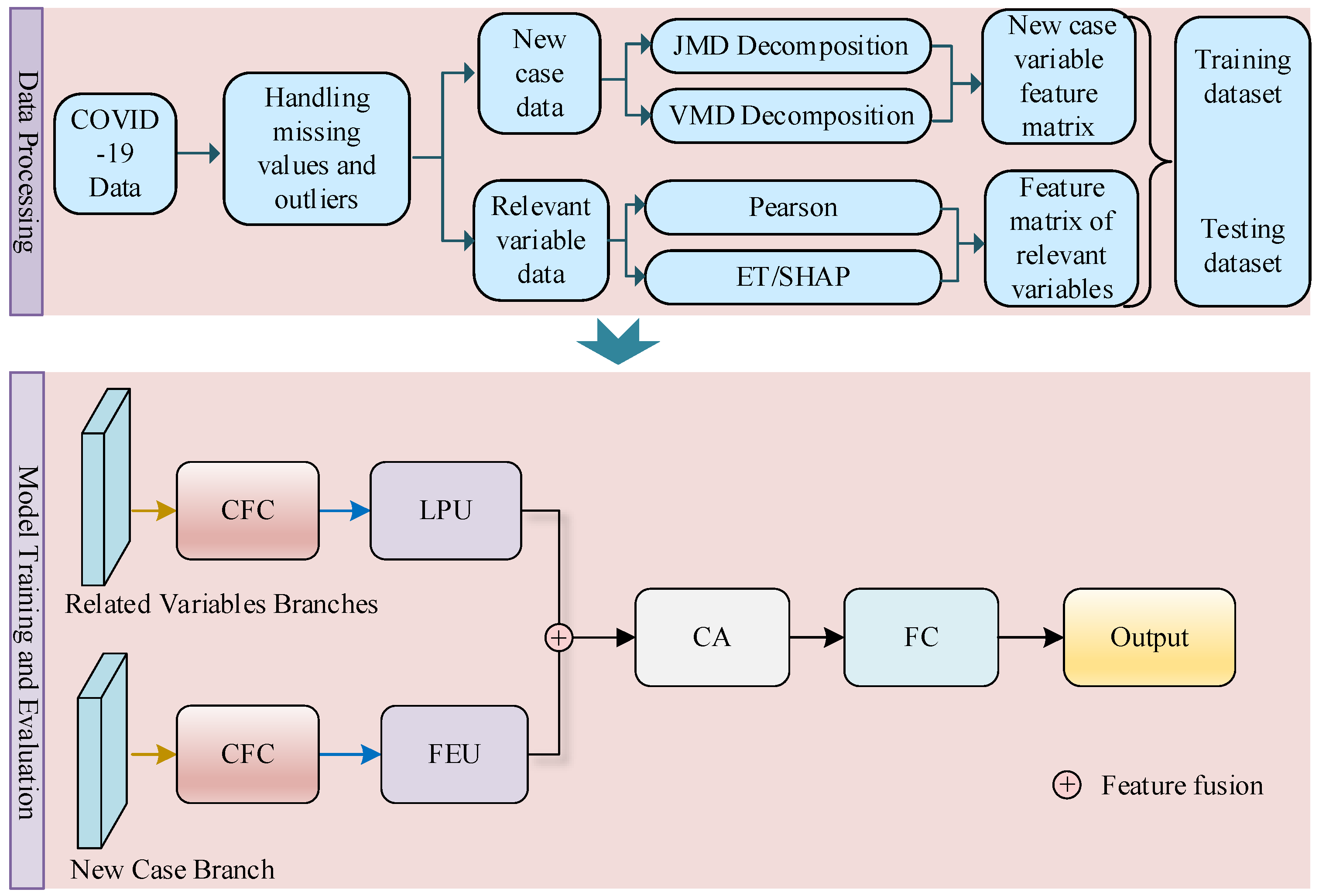
The overall experimental procedure is divided into two core stages: data preprocessing, and model training and evaluation. The complete prediction workflow is illustrated in Figure 9.

Figure 9. Experimental Procedure and Prediction Framework.

4.1. Experimental Data Preprocessing and Sample Construction

In the data preprocessing stage, raw epidemic data are first cleaned, and missing values are imputed via linear interpolation to ensure sequence integrity. Then, the Pearson correlation coefficient between each external factor and the number of new COVID-19 cases is calculated, and nine external factors with absolute correlation coefficients greater than 0.2 are selected as input covariates. All variables are scaled via min–max normalization to eliminate dimensional inconsistency and enhance the model’s ability to capture fine-grained data fluctuations.

After correlation screening and normalization, the feature matrix of correlated variables F_V is constructed as the input of the correlated variable branch. For the new case sequence, the normalized data are further processed via the proposed VMD-JMD hybrid decomposition strategy: the JMD method extracts six subsequences, and the VMD method generates six subsequences. The 12 subsequences are concatenated to form the new case feature matrix F_N, which serves as the input of the new case branch.

To adapt to short-term epidemic forecasting requirements, prediction horizons are set to one-step-, two-steps-, and three-steps-ahead forecasting. The input time window length is uniformly set to 14 for both branches: The new case branch uses a feature matrix of size 14 × 12, which selects the first 14 time steps of the new case feature matrix. The correlated variable branch uses a feature matrix of size 14 × 9, which takes the first 14 time steps of the correlated variable feature matrix. Correspondingly, for one-step forecasting, the model outputs the new case data of the 15th day; for two-step forecasting, it outputs the new case data of the 15th and 16th days; for three-step forecasting, it outputs the new case data from the 15th to 17th day.

The complete dataset is randomly split into a training dataset and a testing dataset at a 7:3 ratio. The training subset accounts for 70% of all time-series samples to provide sufficient data for model fitting and parameter optimization, while the remaining 30% of samples form the testing subset to evaluate the generalization and forecasting performance of the trained model on unseen epidemic data.

4.2. Implementation Details of the CFC-FLCA Forecasting Model

In the training and evaluation stage, the proposed CFC-FLCA model adopts a multi-module collaborative mechanism to efficiently extract and fuse multi-scale temporal features from new case sequences and highly correlated external factors, so as to improve the forecasting accuracy of non-stationary epidemic time series. The mathematical derivation of each module is detailed as follows.

4.2.1. Implementation of the CFC and Gating Mechanism

The CFC module uses a shared backbone network to learn the joint representation of the input feature matrix $\mathit{F}(t)$ and the historical hidden state $\mathit{x}(t-1)$, which avoids redundant computation and accelerates model convergence. Let the backbone parameter be ${\theta }_{\mathrm{back}}$, the input be the concatenation of $\mathit{F}(t)$ and $\mathit{x}(t-1)$, and the output be the shared hidden feature $\mathit{h}(t)$. The computation process is as follows:

$$\mathit{h}(t)=\mathrm{Backbone}\left(\mathrm{concat}\left(\mathit{F}(t),\mathit{x}(t-1)\right);{\theta }_{\mathrm{back}}\right)$$

(6)

where $\mathit{F}\in {ℝ}^{N\times J}$ is the input feature matrix, N is the length of the input time window, and J is the feature dimension. The inputs to the two branches are F_N and F_V, respectively; $\mathit{h}(t)\in {ℝ}^{N\times H}$ is the shared hidden feature, and H is the hidden dimension of the backbone network; $\mathrm{concat}(\cdot )$ denotes the feature concatenation operation along the feature dimension.

Subsequently, the shared features are fed into three independent fully connected head networks to generate three gating-related vectors. The computation is

$$\left\{\begin{array}{c}{\mathit{f}}_t=f\left(\mathit{h}(t);{\theta }_f\right)\\ {\mathit{g}}_t=g\left(\mathit{h}(t);{\theta }_g\right)\\ {\mathit{h}}_t=h\left(\mathit{h}(t);{\theta }_h\right)\end{array}\right.$$

(7)

where ${\mathit{f}}_t$ is the time-constant modulation vector, ${\mathit{g}}_t$ and ${\mathit{h}}_t$ are nonlinear transformation vectors; $f(\cdot )$, $g(\cdot )$ and $h(\cdot )$ represent three independent fully connected nonlinear mapping functions corresponding to the head networks; and ${\theta }_f$, ${\theta }_g$ and ${\theta }_h$ are the trainable parameters of the three head networks, respectively.

To mitigate the vanishing gradient problem and enhance numerical stability for long-sequence modeling tasks, the original exponential decay term in the closed-form solution is replaced by a reverse sigmoid gating mechanism. The gating output is computed as follows:

$${\mathit{\Gamma }}_t=\sigma \left(-{\mathit{f}}_t\odot \Delta t\right)$$

(8)

where $\sigma$ denotes the sigmoid activation function; $\odot$ denotes the Hadamard product; $\Delta t$ is the time step interval between adjacent samples; and ${\mathit{\Gamma }}_t$ is the output of the reverse time gate.

Finally, the hidden state of the current time step is obtained by the weighted fusion of ${\mathit{g}}_t$ and ${\mathit{h}}_t$ via the time gate:

$${\mathit{F}}_{\mathrm{C}}={\mathit{\Gamma }}_t\odot {\mathit{g}}_t+(\mathbf{1}-{\mathit{\Gamma }}_t)\odot {\mathit{h}}_t$$

(9)

where ${\mathit{F}}_{\mathrm{C}}\in {ℝ}^{N\times H}$ is the output feature of the CFC module. For the two branches, the CFC outputs are denoted as new case branch F_C1 and correlated variable branch F_C2, respectively.

4.2.2. Configuration of the Frequency-Domain Enhancement Unit

The output F_C1 of the new case branch from the CFC module is fed into the FEU module. Frequency-domain features are extracted via fast Fourier transform, low-frequency mode filtering, low-rank approximation of frequency-domain linear transformation, and real-imaginary component concatenation and aggregation. The computation process is

$$\left\{\begin{array}{c}\widehat{\mathit{X}}=\mathrm{FFT}\left({\mathit{F}}_{\mathrm{C}1},\dim =1\right)\\ {\widehat{\mathit{X}}}_M=\widehat{\mathit{X}}[:,:M,:]\\ \widehat{\mathit{Y}}={\widehat{\mathit{X}}}_M\cdot {\mathit{W}}_1\cdot {\mathit{W}}_2\cdot {\mathit{W}}_3^{\mathrm{T}}\\ {\mathit{O}}_{\mathrm{FEU}}=\mathrm{GAP}\left(\mathrm{concat}\left(\mathrm{Re}(\widehat{\mathit{Y}}),\mathrm{Im}(\widehat{\mathit{Y}})\right)\right)\end{array}\right.$$

(10)

where $\mathrm{FFT}(\cdot ,\dim =1)$ is the fast Fourier transform operator along the time dimension; $\widehat{\mathit{X}}$ is the complex frequency-domain representation of the time-domain input after Fourier transform; $M$ is the threshold of low-frequency mode filtering; ${\widehat{\mathit{X}}}_M$ is the truncated frequency-domain feature after low-frequency mode filtering; ${\mathit{W}}_1$, ${\mathit{W}}_2$ and ${\mathit{W}}_3$ are the weight matrices of low-rank decomposition for the frequency-domain linear layer, which reduces parameter redundancy compared with the full-rank linear layer; $\mathrm{T}$ denotes the matrix transpose operation; $\widehat{\mathit{Y}}$ is the output feature after frequency-domain linear transformation; $\mathrm{Re}(\cdot )$ and $\mathrm{Im}(\cdot )$ are the real-part and imaginary-part extraction operators for complex tensors, respectively; $\mathrm{GAP}(\cdot )$ denotes the global average pooling operation; ${\mathit{O}}_{\mathrm{FEU}}$ is the final aggregated frequency-domain feature.

4.2.3. Setup of the Legendre Time-Domain Projection Unit

The correlated variable branch takes the CFC output F_C2 as input, and projects it into the Legendre memory space to capture multi-scale temporal dependencies. The calculation process is

$$\left\{\begin{array}{l}{\mathit{C}}_t=\mathit{A}{\mathit{C}}_{t-1}+\mathit{B}\cdot {\mathit{F}}_{\mathrm{C}2}[:,t,:]\hfill \\ {\mathit{C}}_{\mathrm{flat}}=\mathrm{Flatten}({\mathit{C}}_t)\hfill \\ {\mathit{Y}}_{\mathrm{proj}}={\mathit{C}}_{\mathrm{flat}}\cdot {\mathit{W}}_{\mathrm{proj}}+{\mathit{b}}_{\mathrm{proj}}\hfill \\ {\mathit{O}}_{\mathrm{LPU}}=\mathrm{LN}\left({\mathit{Y}}_{\mathrm{proj}}\right)\hfill \end{array}\right.$$

(11)

where A and B are the predefined, non-trainable state transition matrix and input matrix of the Legendre memory unit, determined by the order of Legendre polynomials; ${\mathit{C}}_t$ is the state of the Legendre memory cell at time step t, initialized as a zero vector at $t=0$; $\mathrm{Flatten}(\cdot )$ denotes the feature flattening operation; ${\mathit{W}}_{\mathrm{proj}}$ and ${\mathit{b}}_{\mathrm{proj}}$ are the trainable weight matrix and bias vector of the output linear projection layer, respectively; ${\mathit{Y}}_{\mathrm{proj}}$ is the output feature of the linear projection layer; $\mathrm{LN}(\cdot )$ denotes the layer normalization operation; and ${\mathit{O}}_{\mathrm{LPU}}$ is the final output time-domain feature.

4.2.4. Cross-Attention Fusion Module Deployment

The outputs of the FEU module and the LPU module are fed into the cross-attention module to realize the complementary fusion of frequency-domain and time-domain features. The computation process is

$$\left\{\begin{array}{c}{\mathit{Q}}_F={\mathit{O}}_{\mathrm{FEU}}\times {\mathit{W}}^Q\\ {\mathit{K}}_L={\mathit{O}}_{\mathrm{LPU}}\times {\mathit{W}}^K\\ {\mathit{V}}_L={\mathit{O}}_{\mathrm{LPU}}\times {\mathit{W}}^V\\ {\mathit{F}}_{\mathrm{CA}}=\mathrm{softmax}\left({\displaystyle \frac{{\mathit{Q}}_F\times {{\mathit{K}}_L}^{\mathrm{T}}}{\sqrt{d_k}}}\right){\mathit{V}}_L\end{array}\right.$$

(12)

where ${\mathit{W}}^Q$, ${\mathit{W}}^K$ and ${\mathit{W}}^V$ are the query, key and value weight matrices of the cross-attention module, respectively; ${\mathit{Q}}_F$, ${\mathit{K}}_L$ and ${\mathit{V}}_L$ are the query, key and value matrices corresponding to the cross-attention module, respectively; softmax is the normalization function; $d_k$ is the dimension of the key vector; and ${\mathit{F}}_{\mathrm{CA}}$ is the fused feature sequence output by the cross-attention module.

4.2.5. Output Layer and Prediction Performance Calculation

Finally, the fused feature sequence generated by the cross-attention module is fed into a fully connected layer to obtain the predicted new COVID-19 case values across all target forecasting horizons, and the prediction performance is quantitatively assessed using multiple error metrics.

5. Discussion

This paper designs five sets of experiments: experiments on optimal hyperparameter tuning, Computational Complexity Analysis, comparisons of different decomposition methods, comparisons of different models, and comparisons of data from different countries. Each set of experiments is run 10 times, and the results are averaged to reduce randomness. The experimental platform was based on hardware specifications including a CPU (Intel Core i5-13400F 2.5 GHz), RAM (32 GB), and GPU (RTX 3060 12 G). Deep learning models were built in the PyCharm 2025.1 environment, and the Adam optimization algorithm was used during training to improve convergence efficiency and stability.

5.1. Experiments on Model Training Hyperparameter Settings

Hyperparameter configuration directly determines the model’s training convergence efficiency and final task performance; different combinations can lead to significant differences in prediction accuracy, convergence speed, and stability. Through systematic hyperparameter comparison experiments, it is possible to conduct a side-by-side comparison of the performance of different configurations, precisely identify the optimal hyperparameter combination suited to the target task and dataset, and ensure the model’s accuracy and stability at the training level. See Table 2 for the experimental results of the optimal model parameters and multiple sets of training hyperparameters.

Table 2. Comparison of Experimental Errors in Model Hyperparameter Tuning.

Number	Epoch	Batch	Learning Rate	Runtime/min	Methodology
					EMAE	EMAPE%	ERMSE	R2
1	500	7	0.001	18.50	272.977	7.073	730.369	0.977
2	500	14	0.001	9.16	272.117	7.126	643.058	0.982
3	300	21	0.001	3.13	301.358	7.751	561.010	0.986
4	500	21	0.001	6.03	167.102	5.841	289.779	0.996
5	500	21	0.0001	6.03	262.059	6.556	465.113	0.990
6	800	21	0.001	9.34	229.794	6.515	427.785	0.992
7	500	28	0.001	4.50	300.351	7.413	546.548	0.987
8	800	28	0.001	8.04	286.708	6.774	529.362	0.988

As summarized in Table 2, the proposed model delivers the most stable convergence and superior forecasting performance with an initial learning rate of 0.001. By contrast, a smaller learning rate of 0.0001 hinders parameter updating speed, slows training convergence, and triggers the conspicuous deterioration of prediction quality, reflected by prominent elevations across all error indicators.

With the learning rate fixed at 0.001 and batch size set to 21, extending training epochs from 300 to 500 effectively suppresses forecasting errors and markedly elevates the overall fitting capability. Nevertheless, further expanding iterations to 800 brings no performance benefits: all error metrics rebound noticeably alongside degraded fitting effects, while the total training runtime rises from 6.03 min to 9.34 min, introducing unnecessary computational overhead.

Regarding batch size ablation under a constant learning rate of 0.001 and 500 training epochs, larger batches consistently shorten total training time. When the batch size grows from 7 to 21, the runtime drops sharply from 18.50 min to 6.03 min, accompanied by continuous performance improvements. However, pushing the batch size to 28 further cuts runtime to 4.50 min at the cost of weakened generalization: all error values rise substantially and prediction fitting capacity degrades accordingly. On the other hand, an excessively tiny batch size, though capable of eventual convergence, drastically prolongs training duration, which incurs unaffordable time costs and limits the model’s practical engineering deployment value.

In aggregate, the hyperparameter combination of 500 training epochs, a batch size of 21, and a learning rate of 0.001 is identified as the optimal configuration for the proposed forecasting task. This set of hyperparameters enables the model to attain state-of-the-art prediction accuracy while maintaining a moderate training runtime, striking a favorable trade-off between forecasting performance and practical engineering efficiency.

5.2. Computational Complexity Analysis

To quantitatively evaluate the parameter scale and computational overhead of our proposed architecture, we design a series of controlled comparative ablation experiments based on the dual-branch CFC. First, lightweight LPU and FEU are integrated into the vanilla dual-branch CFC to build the CFC-FL variant. On this basis, a cross-branch cross-attention module is further embedded into CFC-FL to construct the final complete forecasting model. This stepwise module stacking strategy enables us to quantify the incremental parameters and computational load brought by each individual component. Classical time-series forecasting models including CNN, LSTM and temporal convolutional network (TCN) are selected as external baselines for horizontal comparison. Three metrics are adopted for evaluation: trainable parameters (Params), floating-point operations (FLOPs), and end-to-end inference runtime under the 1-step-ahead forecasting setting. The results reflect the trade-off between prediction performance gain and computational resource consumption of the proposed model.

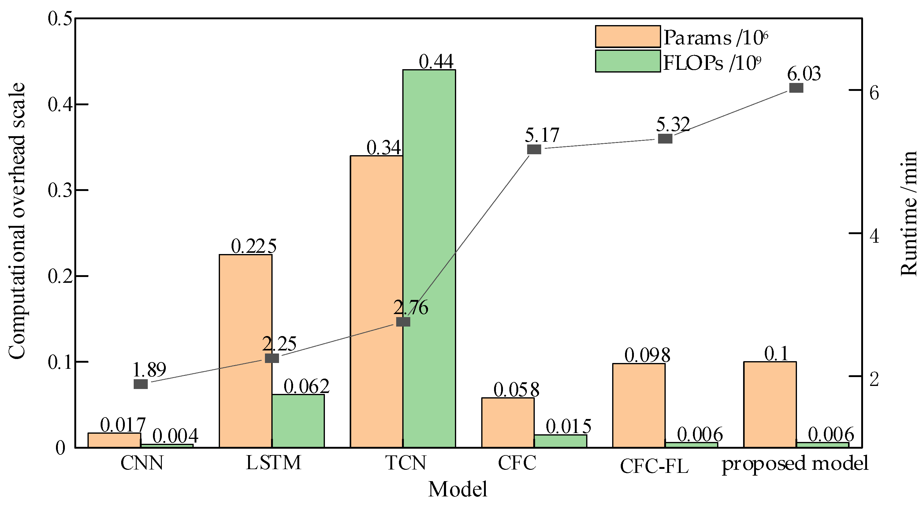
As shown in the experimental results in Table 3 in terms of prediction accuracy, the proposed model achieves far superior fitting ability compared with CNN, LSTM and TCN. From the perspective of computational overhead, CNN holds the minimal parameter count 0.017 × 10⁶ and FLOPs 0.004 × 10⁹, with the shortest inference runtime of 1.89 min, yet its forecasting precision is severely insufficient. LSTM and TCN bring a moderate accuracy promotion but introduce drastically increased computational burden: TCN requires the maximum trainable parameters 0.340 × 10⁶, the highest FLOPs 0.440 × 10⁹ and the longest inference time among all traditional baselines, which severely limits its deployment efficiency. By contrast, our model only consumes 0.100 × 10⁶ trainable parameters and 0.006 × 10⁹ FLOPs, which are significantly lower than LSTM and TCN, proving that the proposed architecture avoids the redundant parameter stacking and heavy calculation of recurrent and temporal convolution frameworks.

Table 3. Comparison of the Computational Complexity and Training Costs of Models.

Model	EMAE	EMAPE%	ERMSE	R2	Params/106	FLOPs/109	Runtime/min
CNN	1640.539	62.921	2427.266	0.747	0.017	0.004	1.89
LSTM	1476.437	48.061	2213.968	0.791	0.225	0.062	2.25
TCN	1320.411	69.708	1580.595	0.893	0.340	0.440	2.76
CFC	338.684	8.905	713.351	0.978	0.058	0.015	5.17
CFC-FL	220,120	6.783	523.432	0.981	0.098	0.006	5.32
proposed model	167.102	5.841	289.779	0.996	0.100	0.006	6.03

Compared with the dual-branch CFC, the CFC-FL variant integrated with LPU and FEU modules slightly increases trainable parameters, and extends inference runtime marginally from 5.17 min to 5.32 min. This minor computational increment delivers moderate accuracy gains, which validates the lightweight optimization effect of the LPU and FEU. On this basis, the proposed model further embeds a cross-attention module into the CFC-FL framework. Only a tiny growth of parameters and a slight rise in inference time are observed, with FLOPs remaining constant at 0.006 × 10⁹. The negligible extra computational overhead brings substantial forecasting performance promotion and all error metrics achieve the minimum values across all comparison models. This contrast proves that the introduced cross-branch cross-attention module imposes almost no extra computational burden, and the trivial added runtime cost is fully worth the prominent accuracy improvement.

Synthesizing all prediction and computational metrics, the proposed model achieves an optimal trade-off between forecasting performance and computational resource consumption. When benchmarked against conventional time-series baselines CNN, LSTM, TCN, the proposed method obtains far superior prediction fitting capacity despite its marginally longer inference latency. In particular, compared with the heavyweight recurrent and temporal convolution models LSTM and TCN, our framework has far fewer trainable parameters and much lower floating-point computation volume, which endows it with a prominent lightweight deployment capability for real-world forecasting tasks. Overall, the proposed dual-branch CFC architecture with cross-attention attains state-of-the-art prediction accuracy under constrained computational cost, fully verifying its high efficiency and lightweight design superiority.

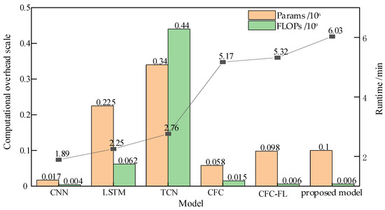
As shown in the experimental results in Figure 10, the left vertical axis corresponds to the magnitude of trainable parameters (10⁶, orange bars) and FLOPs (10⁹, green bars). The right vertical axis represents inference runtime (min, black polyline). Traditional CNN, LSTM and TCN show a positive correlation between parameter scale, calculation volume and inference time, with TCN owning the heaviest computational burden. The ablation chain CFC → CFC-FL → proposed model verifies that LPU, FEU and cross-attention modules introduce minimal extra computational overhead, demonstrating the lightweight design advantage of the dual-branch CFC framework with cross-attention.

Figure 10. Comparison of model computational complexity and inference cost.

5.3. Comparative Experiments Using Different Decomposition Methods

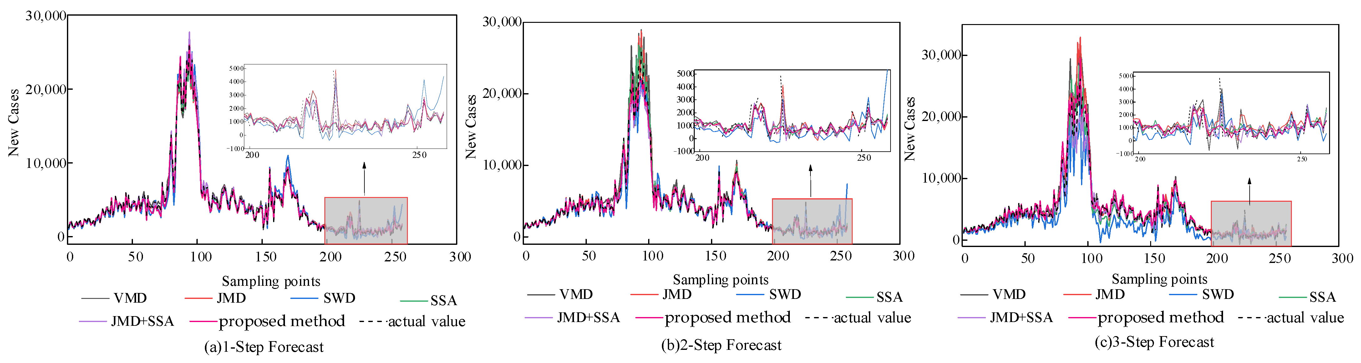
To verify the superiority of the proposed hybrid decomposition strategy over single-decomposition methods in terms of prediction performance, the original sequences were first preprocessed using JMD and VMD, respectively, and the resulting modal components were fed into the dual-branch CFC-FLCA network for prediction. To further evaluate the effectiveness of this hybrid approach, Swarm Decomposition (SWD) and Singular Spectrum Analysis (SSA) were introduced as additional control methods. Comparative experiments were conducted by combining all these decomposition algorithms with the dual-branch prediction framework. The results of each method under three prediction strides (1, 2, and 3) are shown in Table 3 using multi-dimensional error evaluation metrics. Figure 10 displays the prediction curves from the decomposition comparison experiments, analyzing the stability and performance differences in various decomposition strategies in prediction.

As shown in the experimental results in Table 4 and Figure 11, the proposed hybrid modal decomposition method integrates the complementary advantages of two decomposition algorithms, and outperforms all single-decomposition and other combined decomposition methods under all prediction horizons across every evaluation metric. This reflects its ability to extract multi-scale features and suppress noise for non-stationary epidemic time series.

Table 4. Comparison of Prediction Errors from Different Decomposition Methods.

Decomposition Method	EMAE			EMAPE%			ERMSE			R2
	1-Step	2-Step	3-Step	1-Step	2-Step	3-Step	1-Step	2-Step	3-Step	1-Step	2-Step	3-Step
VMD	471.176	685.352	802.466	21.938	24.155	29.052	718.225	1171.607	1544.534	0.978	0.941	0.898
JMD	170.656	350.122	683.35	8.36	12.745	26.918	309.226	656.621	1364.937	0.99	0.981	0.92
SWD	529.042	589.138	1440.76	24.283	26.737	41.983	735.578	1004.781	2157.678	0.976	0.957	0.8019
SSA	179.151	377.269	534.858	9.6378	13.378	17.253	391.639	700.644	922.309	0.983	0.979	0.963
JMD + SSA	171.575	339.871	527.236	8.481	9.56	16.357	316.881	745.83	963.388	0.99	0.976	0.96
proposed method	167.102	308.553	514.808	5.841	10.23	15.546	289.779	601.867	884.605	0.996	0.984	0.966

Figure 11. Comparison of Predicted Trends from Different Decomposition Experiments.

Figure 11 presents prediction curves of all decomposition schemes under one-step, two-step and three-step forecasting settings. All models show increasing prediction deviation as the prediction steps expand, which conforms to the common error accumulation rule of multi-step forecasting. The curve of the proposed method overlaps most closely with ground-truth values at all forecasting strides.

Taking the challenging three-step forecast as an example, standalone VMD yields E_MAE is 802.466, E_MAPE is 29.052, E_RMSE is 1544.534 and R² is 0.898, while the proposed method reduces the three error metrics by 35.8%, 46.5% and 42.7%, respectively, and lifts R² to 0.966, achieving prominent fitting improvement. The superiority is more obvious in one-step forecasting: E_MAPE drops from 21.938 (single VMD) to 5.841, with a relative error reduction over 73.3%. The hybrid decomposition retains VMD’s ability to filter high-frequency noise and leverages JMD’s strength in capturing low-frequency trends, remedying the inherent defects of single decomposition strategies.

The proposed decomposition also surpasses the JMD + SSA combined scheme on all metrics. For three-step prediction, its E_RMSE reaches 884.605, 8.2% lower than the 963.388 of JMD + SSA. Meanwhile, E_MAPE falls by 5.0%, E_MAE declines by 2.4%, and R² rises from 0.960 to 0.966. The marginal performance gain of simple modal concatenation indicates that direct stacking introduces redundant modal information and fails to realize effective feature complementarity.

5.4. Comparative Experiment of Different Models

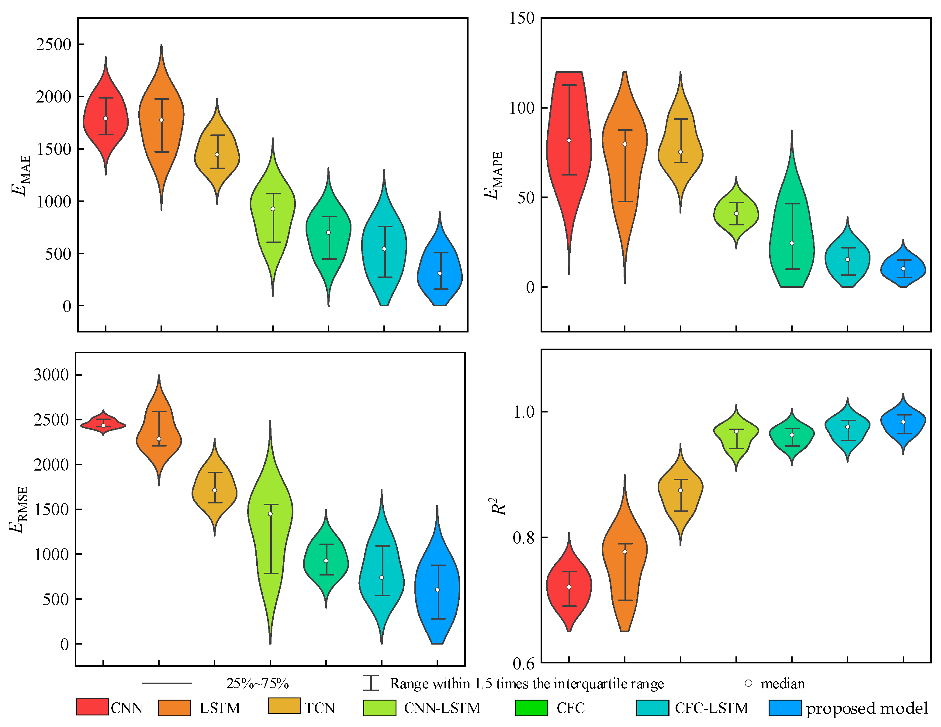
To validate the advantages of the proposed dual-branch deep learning model, CFC-FLCA, this paper selected several models for comparison. These include CNN, LSTM, TCN, CFC, and the combined prediction models CNN-LSTM and CFC-LSTM. To compare the generalization capabilities of each model, data processed through mixed decomposition and normalization was input into the various combined new case prediction models, and predictions were performed for one, two, and three steps. The specific experimental results are shown in Table 5 and Figure 12.

Table 5. Comparison of Prediction Errors from Different Model Methods.

Model	EMAE			EMAPE%			ERMSE			R2
	1-Step	2-Step	3-Step	1-Step	2-Step	3-Step	1-Step	2-Step	3-Step	1-Step	2-Step	3-Step
CNN	1640.539	1791.539	1990.747	62.921	81.831	112.919	2427.266	2435.14	2509.295	0.747	0.721	0.692
LSTM	1476.437	1775.33	1980.873	48.061	79.743	87.812	2213.968	2286.371	2593.904	0.791	0.777	0.701
TCN	1320.411	1446.12	1634.258	69.708	75.308	94.049	1580.595	1714.048	1917.729	0.893	0.875	0.843
CNN-LSTM	614.209	925.769	1078.535	35.195	41.004	47.666	793.466	1450.237	1560.365	0.973	0.969	0.942
CFC	455.913	700.276	862.372	10.448	24.514	46.838	779.321	924.676	1120.001	0.974	0.963	0.946
CFC-LSTM	279.357	542.531	764.226	7.207	15.338	22.459	548.255	740.458	1101.18	0.987	0.976	0.955
proposed model	167.102	308.553	514.808	5.841	10.23	15.546	289.779	601.867	884.605	0.996	0.984	0.966

Figure 12. Comparison of Violin Images with Cases Under Different Error Types as Predicted by Various Models.

As shown in Table 5, the proposed CFC-FLCA dual-branch model yields optimal forecasting results across one-step, two-step and three-step horizons, surpassing conventional time-series baselines and other CFC derivative variants comprehensively. Taking the challenging three-step long-term forecasting task as an example, the E_RMSE of the proposed model equals 884.605, which is 64.7%, 65.9%, 53.9%, 43.3%, 21.0% and 19.7% lower than CNN, LSTM, TCN, CNN-LSTM, vanilla CFC and CFC-LSTM separately. Meanwhile, its E_MAPE drops to 15.546, and the corresponding R² reaches 0.966 to deliver superior fitting capabilities. Such superiority becomes more prominent under short-term one-step forecasting: the model achieves E_MAE is 167.102 and peak R² is 0.996, with a 40.2% reduction in E_MAE relative to the suboptimal CFC-LSTM. These outcomes verify that the collaborative design of spatiotemporal dual branches and cross-attention fusion breaks through the performance limitations of single-branch temporal prediction networks.

Figure 12 provides violin plots to visualize the overall error distribution of all comparative models. For all four evaluation metrics, the distribution corresponding to the proposed model presents the narrowest shape, the minimum median error, and the smallest interquartile range (25–75%) and 1.5 × IQR boundary. This feature implies that prediction errors of most samples are restrained within a tight interval without severe extreme outliers. By contrast, classic models including CNN and LSTM display widely scattered error distributions accompanied by massive outliers, which trigger violent fluctuations in prediction outputs. Although CFC and CFC-LSTM alleviate this instability to a certain degree, their error concentration still cannot match that of the CFC-FLCA model.

Consistent with the universal error accumulation law of multi-step forecasting, error metrics of all models rise continuously as prediction steps extend from one step to three steps. Among all candidates, the proposed model shows the mildest performance attenuation: its E_MAPE only rises by 166.2%, which is far below the 211.6% growth of CFC-LSTM. This characteristic confirms its outstanding long-range generalization and robustness.

5.5. Experiment Comparing Data Across Different Countries

To further verify the cross-regional generalization of the proposed CFC-FLCA model based on the primary Irish dataset, datasets from Belgium and the Czech Republic are selected for supplementary validation, covering the period from 28 February 2020 to 19 June 2022. The selection is mainly based on three considerations:

(1) The time spans of the three datasets are highly similar, enabling a unified hybrid modal decomposition and preprocessing pipeline to be applied to all datasets, which ensures experimental consistency and comparability.

(2) The public epidemic data of Belgium and the Czech Republic have few missing values and standardized statistical calibers, with reliable data quality suitable for quantitative comparative experiments.

(3) The three countries show distinct epidemic fluctuation patterns, peak magnitudes and transmission dynamics, which can fully test the model’s adaptability to different regional prevalence scenarios and effectively verify its robustness.

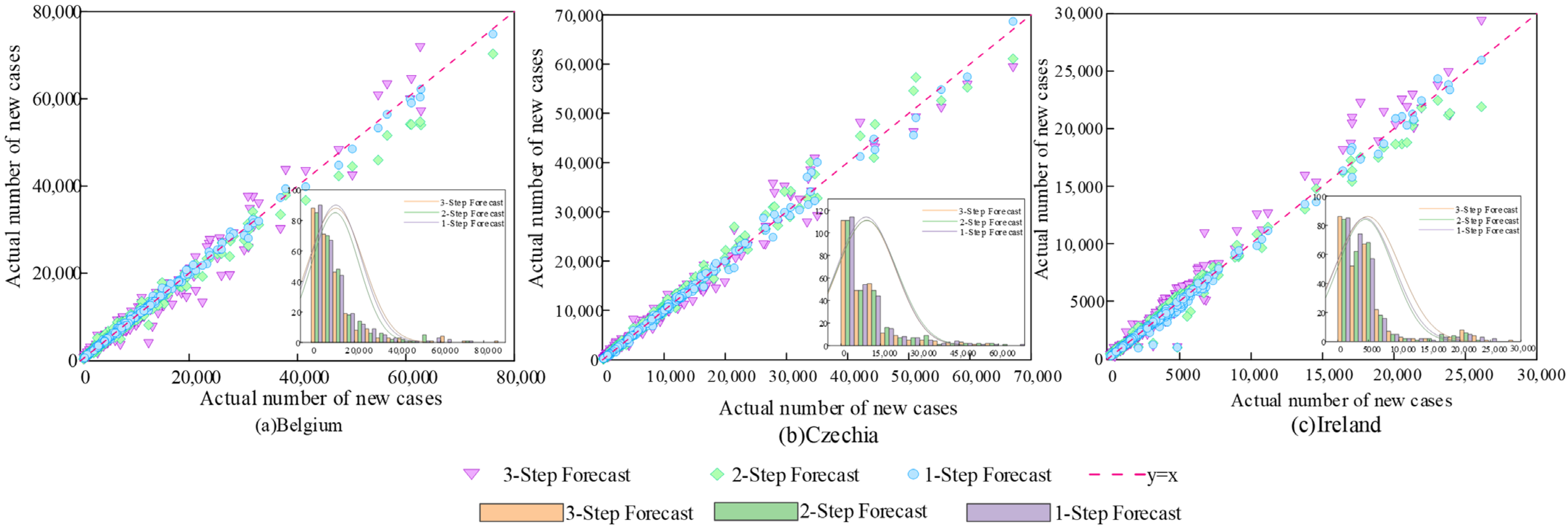
All datasets are uniformly preprocessed and split into 70% training and 30% test sets. All models perform one-step, two-step and three-step forecasting under identical experimental conditions, with the results presented in Table 6 and Figure 13.

Table 6. Comparison of Prediction Errors in Data Experiments Across Different Countries.

Data	EMAE			EMAPE%			ERMSE			R2
	1-Step	2-Step	3-Step	1-Step	2-Step	3-Step	1-Step	2-Step	3-Step	1-Step	2-Step	3-Step
Belgium	321.654	724.559	911.674	3.424	8.78	10.023	548.634	1611.542	1825.463	0.997	0.982	0.979
Czechia	353.742	639.671	833.647	9.581	11.612	18.864	798.129	1211.718	1783.715	0.994	0.988	0.966
Ireland	167.102	308.553	514.808	5.841	10.23	15.546	289.779	601.867	884.605	0.996	0.984	0.966

Figure 13. Comparison of Data Fits Across Countries.

As shown in Table 6, the CFC-FLCA model proposed in this paper demonstrates excellent predictive performance and strong cross-country generalization capabilities across different national datasets. Taking the Belgian dataset as an example, the one-step prediction achieved an E_MAE of only 321.654, an E_MAPE as low as 3.424, an E_RMSE of 548.634, and an R² as high as 0.997. For the Irish dataset, due to the relatively small number of cases, the model’s prediction accuracy improved further: the E_MAE for a one-step forecast was only 167.102, the E_RMSE was 289.779, and R² reached 0.996; even on the Czech dataset, where the characteristics of pandemic fluctuations differ, the model’s R² for a one-step forecast remained at a high level of 0.994.

The model demonstrated exceptional performance stability in multi-step forecasting tasks; although prediction accuracy decreased systematically as the forecast horizon increased, it remained at a high level. Taking the Belgian dataset as an example, from one-step to three-step forecasting, E_MAE increased from 321.654 to 911.674, E_MAPE rose from 3.424 to 10.023, and E_RMSE increased from 548.634 to 1825.463, yet the coefficient of determination R² remained as high as 0.979; for the Irish dataset, the three-step prediction E_MAE was only 514.808, and E_RMSE was 884.605, and R² remained at 0.966. Although the three-step prediction E_MAPE for the Czech dataset was 18.864, its R² still reached 0.966, indicating that the model could still accurately capture the overall trend of the epidemic.

Analysis of Figure 13 reveals that the scatter plot of observed and predicted values, along with the error distribution analysis, further validates the reliability and stability of the model’s predictions. The scatter plot shows that all data points from the one-step, two-step, and three-step predictions are tightly clustered around the y = x diagonal line, with virtually no outliers showing significant deviation, indicating a strong linear correlation between the model’s predictions and the observed values. The embedded error distribution histogram shows that the errors for all prediction horizons exhibit a right-skewed unimodal distribution, with the prediction errors for the vast majority of samples concentrated around 0, and the proportion of samples with large errors being extremely low. These findings highlight the CFC-FLCA model’s advantage in capturing the complex nonlinear characteristics of the epidemic. The model exhibits neither systematic overestimation nor systematic underestimation biases; its prediction results are accurate and reliable, capable of providing data support for epidemic prevention and control decisions in different countries.

6. Conclusions

Based on VMD-JMD hybrid modal decomposition, CFC, cross-attention mechanisms, and a dual-branch time–frequency input approach, this paper proposes a CFC-FLCA hybrid forecasting model for predicting new cases. Through experiments, the following conclusions were drawn:

(1) By preprocessing new case data using two complementary modal decomposition methods—VMD and JMD—the original non-stationary incidence sequence is adaptively decomposed into multiple multiscale modal components with clear physical significance. Specifically, VMD effectively separates the high-frequency random noise components in the sequence, while JMD accurately captures the long-term trends and dominant periodic characteristics of the epidemic. The combination of these two methods significantly mitigates the non-stationarity, non-linearity, and random fluctuations in the raw data, thereby improving the input quality and robustness of subsequent prediction models at the data source.

(2) A forecasting network integrating time-domain and frequency-domain input information is constructed. The dual-path CFC backbone, leveraging the inherent long-term memory characteristics of continuous-time differential equations, effectively addresses the gradient vanishing issue and limited local receptive fields of traditional models. The LPU extracts robust time-domain evolutionary features through orthogonal basis transformation, while the FEU uncovers latent periodic patterns that are difficult for traditional time-domain methods to capture. The cross-attention mechanism dynamically learns the importance weights of time–frequency-domain features, enabling adaptive deep integration of information across different dimensions and ultimately achieving precision predictions of new cases.

(3) Compared to traditional time-series models such as CNN, LSTM, and TCN, as well as mainstream hybrid models like CNN-LSTM, CFC, and CFC-LSTM, the CFC-FLCA model proposed in this paper achieves the best overall prediction performance across all prediction horizons. Particularly in the most challenging three-step prediction task, the model maintained high accuracy and stability. An error distribution analysis of the violin plot further validated the consistency and reliability of the model’s predictions, fully demonstrating the feasibility of this method in disease time-series prediction tasks.

(4) Nevertheless, this study still has certain limitations. First, the VMD-JMD hybrid decomposition adopted in this work uses empirically set modal parameters, which cannot be adaptively adjusted according to the fluctuation characteristics of input sequences, resulting in insufficient robustness of feature extraction when dealing with abrupt changes in the epidemic. Second, the core hyperparameters of the prediction network are determined through manual debugging, and there is a lack of dynamic optimization mechanism synchronized with the evolution of the epidemic, which weakens the model’s adaptability to time-varying transmission dynamics. Third, the current verification is only carried out on COVID-19 case data, and the performance of the proposed framework in other infectious disease prediction tasks remains to be explored, which restricts the popularization and application of the method.

(5) In future research, targeted optimization will be conducted around the above shortcomings:

① More advanced adaptive signal decomposition algorithms will be introduced to optimize the modal decomposition effect, further improving the precision and robustness of multi-scale feature extraction.

② An intelligent parameter optimization mechanism will be explored to realize dynamic adaptive adjustment of model parameters along with epidemic changes, enhancing the model’s ability to respond to sudden transmission fluctuations.

③ The time–frequency hybrid forecasting framework will be extended to other infectious disease trend prediction scenarios to verify its generalizability, so as to provide more reliable technical support for public health decision-making.

References

- Gates, B. Responding to COVID-19—A once-in-a-century pandemic? N. Engl. J. Med. 2020, 382, 1677–1679. [Google Scholar] [CrossRef] [Scilit] [PubMed]
- Portus, H.M.; Ban, M.J.; Kim, K.; Cho, K.H.; Kim, S.; Kim, J.H.; Kang, J.-H. Temporal fusion transformer-based forecasting of COVID-19 infection trends using environmental indicators. J. Hazard. Mater. 2026, 512, 141381. [Google Scholar] [CrossRef] [Scilit]
- Shi, Y.; Zhu, X.; Zhu, X.; Cheng, B.; Zhong, Y. Kalman filter-based epidemiological model for post-COVID-19 era surveillance and prediction. Sensors 2025, 25, 2507. [Google Scholar] [CrossRef] [Scilit] [PubMed]
- Wang, Z.A.; Xu, Z.S.; Lin, L.D. Review of COVID-19 propagation prediction methods. Comput. Eng. Appl. 2023, 59, 49–61. [Google Scholar]
- Li, H.; Duan, D.G.; Tao, X.G.; Chen, E.; Gao, S.T. Review on infectious disease dynamics models and their applications in COVID-19 epidemic simulation and prediction. Chin. Med. Equip. J. 2020, 41, 7–12. [Google Scholar]
- Dudukcu, H.V.; Taskiran, M.; Taskiran, Z.G.C.; Yildirim, T. Temporal convolutional networks with RNN approach for chaotic time series prediction. Appl. Soft Comput. 2023, 133, 109945. [Google Scholar] [CrossRef] [Scilit]
- Monllor, P.; Su, Z.; Gabrielli, L.; Taltavull de La Paz, P. COVID-19 infection process in Italy and Spain: Are data talking? Evidence from ARMA and vector autoregression models. Front. Public Health 2020, 8, 550602. [Google Scholar] [CrossRef] [Scilit] [PubMed]
- Özen, F. Random forest regression for prediction of COVID-19 daily cases and deaths in Turkey. Heliyon 2024, 10, e25746. [Google Scholar] [CrossRef] [Scilit] [PubMed]
- Rath, S.; Tripathy, A.; Tripathy, A.R. Prediction of new active cases of coronavirus disease (COVID-19) pandemic using multiple linear regression model. Diabetes Metab. Syndr. Clin. Res. Rev. 2020, 14, 1467–1474. [Google Scholar] [CrossRef] [Scilit]
- Vadyala, S.R.; Betgeri, S.N.; Sherer, E.A.; Amrutur, A. Prediction of the number of COVID-19 confirmed cases based on K-means-LSTM. Array 2021, 11, 100085. [Google Scholar] [CrossRef] [Scilit] [PubMed]
- Shahid, F.; Zameer, A.; Muneeb, M. Predictions for COVID-19 with deep learning models of LSTM, GRU and Bi-LSTM. Chaos Solit. Fractals 2020, 140, 110212. [Google Scholar] [CrossRef] [Scilit]
- Gautam, Y. Transfer learning for COVID-19 cases and deaths forecast using LSTM network. ISA Trans. 2022, 124, 41–56. [Google Scholar] [CrossRef] [Scilit] [PubMed]
- Jin, W.Q.; Dong, S.Q.; Yu, C.Q.; Luo, Q.Q. A data-driven hybrid ensemble AI model for COVID-19 infection forecast using multiple neural networks and reinforced learning. Comput. Biol. Med. 2022, 146, 105560. [Google Scholar] [CrossRef] [Scilit] [PubMed]
- Zhang, C.; Sun, G.X. COVID-19 Spreading Prediction Model Based on a Multi-Head Self-Attention Mechanism. Res. Sq. 2024, 2024051234. [Google Scholar] [CrossRef] [Scilit] [PubMed]
- Samuelsson, H. Enhancing Skin Cancer Classification: A Hybrid Convolutional Neural Network and Closed-Form Continuous-Time Approach for Improved Accuracy and Efficiency. Master’s Thesis, KTH Royal Institute of Technology, Stockholm, Sweden, 2024. [Google Scholar]
- Lechner, M.; Hasani, R. Learning long-term dependencies in irregularly-sampled time series. In Proceedings of the 2020 IEEE 23rd International Conference on Information Fusion (FUSION), Virtual, 6–9 July 2020; pp. 1–8. [Google Scholar]
- Zhao, Q.; Zheng, Z.T. Prediction of COVID-19 in BRICS countries: An integrated deep learning model of CEEMDAN-R-ILSTM-Elman. Comput. Math. Methods Med. 2022, 2022, 1566727. [Google Scholar] [CrossRef] [Scilit] [PubMed]
- Liu, S.; Wan, Y.; Yang, W.; Tan, A.; Jian, J.; Lei, X. A hybrid model for coronavirus disease 2019 forecasting based on ensemble empirical mode decomposition and deep learning. Int. J. Environ. Res. Public Health 2023, 20, 617. [Google Scholar]
- Yang, H.; Liu, H.; Li, G. A novel prediction model based on decomposition-integration and error correction for COVID-19 daily confirmed and death cases. Comput. Biol. Med. 2023, 156, 106674. [Google Scholar] [CrossRef] [Scilit] [PubMed]
- Oană, I.; Mihăilă-Pințoiu, B.-E.; Hâncean, M.-G. COVID-19 Integrated Dataset: A Unique Blend of Social Dynamics and Weather Conditions; Version 2; Zenodo: Geneva, Switzerland, 2023. [Google Scholar] [CrossRef]
- Wang, Z.; Guo, L.; Gong, H.; Li, X.; Zhu, L.; Sun, Y.; Chen, B.; Zhu, X. Land subsidence simulation based on extremely randomized trees combined with Monte Carlo algorithm. Comput. Geosci. 2023, 178, 105415. [Google Scholar] [CrossRef] [Scilit]
- Nazari, M.; Korshøj, A.R.; Rehman, N.U. Jump plus AM-FM mode decomposition. IEEE Trans. Signal Process. 2025, 73, 1081–1093. [Google Scholar] [CrossRef] [Scilit]
- Dragomiretskiy, K.; Zosso, D. Variational mode decomposition. IEEE Trans. Signal Process. 2013, 62, 531–544. [Google Scholar] [CrossRef] [Scilit]
- Zhang, X.-S.; Vynnycky, E.; Charlett, A.; De Angelis, D.; Chen, Z.; Liu, W. Transmission dynamics and control measures of COVID-19 outbreak in China: A modelling study. Sci. Rep. 2021, 11, 2652. [Google Scholar] [CrossRef] [Scilit] [PubMed]
- Hasani, R.; Lechner, M.; Amini, A.; Liebenwein, L.; Ray, A.; Tschaikowski, M.; Teschl, G.; Rus, D. Closed-form continuous-time neural networks. Nat. Mach. Intell. 2022, 4, 992–1003. [Google Scholar] [CrossRef] [Scilit]
- Zhou, T.; Ma, Z.; Wang, X.; Wen, Q.; Sun, L.; Yao, T.; Yin, W.; Jin, R. FiLM: Frequency improved Legendre memory model for long-term time series forecasting. arXiv 2022, arXiv:2205.08897. [Google Scholar] [CrossRef] [Scilit]
- Gu, A.; Dao, T.; Ermon, S.; Rudra, A.; Ré, C. HiPPO: Recurrent memory with optimal polynomial projections. In Advances in Neural Information Processing Systems 33 (NeurIPS 2020); Curran Associates: Red Hook, NY, USA, 2020; pp. 1474–1487. [Google Scholar]
Disclaimer/Publisher’s Note: The statements, opinions and data contained in all publications are solely those of the individual author(s) and contributor(s) and not of MDPI and/or the editor(s). MDPI and/or the editor(s) disclaim responsibility for any injury to people or property resulting from any ideas, methods, instructions or products referred to in the content. |
© 2026 by the authors. Licensee MDPI, Basel, Switzerland. This article is an open access article distributed under the terms and conditions of the Creative Commons Attribution (CC BY) license.