Belief-Guided Homeostatic Estimation for Regime Adaptation in Multi-Layer Industrial Network Scheduling

Abstract

Scheduling in multi-layer industrial networks must remain stable even when the feedback mechanism of the environment changes inside a single production episode. The system can switch between a step-continuous regime with dense process feedback and a task-driven regime with sparse milestone feedback, so that the same state requires different behaviour before and after the switch. A regime-oblivious policy may therefore optimise the wrong action preference after a switch. We formulate this setting as a mode-switched multi-industrial-chain Markov decision process (MS-MIC-MDP) and prove that a single fixed action preference is necessarily suboptimal in at least one regime. We then propose BHERA, a belief-guided homeostatic estimation framework for regime adaptation. BHERA builds cross-layer representations, performs structured variational inference of slow and fast latent beliefs, estimates the posterior probability of the task-driven regime, and uses that posterior to regulate sample weights, entropy strength, return-prediction emphasis, and latent information capacity. A homeostatic feedback rule on the Kullback–Leibler (KL) divergence keeps the latent representation informative without allowing uncontrolled information growth, and we analyse it as a two-timescale stochastic approximation with an associated convergence argument and a per-iteration complexity bound. Experiments in a multi-layer industrial scheduling simulator show that BHERA achieves higher return, lower cost, and higher utility than CReSCENT, HiTAC-MuSE, Informed Switching, and WToE across all tested perturbations, with paired statistical tests confirming significance. Expanded ablations and parameter-sensitivity studies confirm the importance of regime belief, regime-balanced weighting, bootstrap prediction, homeostatic capacity control, and the dual-timescale latent split.

1. Introduction

Modern industrial production is increasingly organised as a multi-layer network rather than as a single isolated shop floor. Sensing, transport, buffering, and processing are distributed across coupled layers, and the cyber-physical integration promoted by Industry 4.0 connects these layers into one networked system [1,2]. Surveys of multi-factory and networked production show that dispatching decisions in such systems depend on transport delays, finite buffers, cross-site constraints, and heterogeneous capacity, so that a locally good choice in one layer can be globally poor once its downstream effects appear [3]. Because the network state changes at every step while the consequences of a decision are revealed much later, scheduling in these systems is a sequential decision problem under uncertainty rather than a static assignment problem. Recent work on multiplex networked industrial chains makes the same point: task migration and chain-disruption risk have to be handled online under shifting operating conditions [4,5].

Deep reinforcement learning (RL) has become a natural tool for this problem because it can adapt a dispatching policy from simulation and online interaction instead of relying on a fixed analytical model [6,7]. Most learning-based schedulers, however, assume that the feedback mechanism is fixed for the whole episode. This paper studies a harder and, in practice, common situation in which the feedback mechanism itself switches inside a single episode. During a step-continuous regime, every decision produces dense process-level feedback. During a task-driven regime, reward is released only when a structural milestone is reached. The same state can therefore require different behaviour depending on the current regime: a locally efficient dispatching choice is appropriate when feedback is dense, while a broader structural exploration choice is appropriate when reward is delayed.

This within-episode regime switch makes training non-stationary. The reward scale changes, the useful time horizon changes, and the gradient direction changes. A scheduler that assumes one fixed feedback mechanism is likely to drift after a switch. Cross-layer coordination methods can reduce conflicts under continuous feedback, but they are not designed to detect when the feedback semantics have changed. Intrinsic-motivation methods can help during sparse milestones, but they may keep injecting exploratory pressure after the system returns to a dense regime. Trigger-based exploration methods learn when to switch behaviour [8,9], yet their triggers often react after value inconsistency has already appeared.

This difficulty matters directly to engineering practice. A production scheduler that silently mis-weights its updates after a regime switch will either over-explore and waste capacity when feedback is already dense, or under-explore and stall when reward becomes delayed. In both cases, the operator sees unstable throughput, fluctuating cost, and a controller that must be retuned by hand whenever the operating mode changes. A method that infers the current feedback regime and adjusts its own learning pressure removes this manual retuning, keeps resource use controlled, and gives more predictable behaviour across operating modes. The belief-guided homeostatic view is attractive for the applied community precisely because it turns an implicit and fragile design choice, namely how strongly to explore right now, into an explicit quantity that is estimated from data and regulated by feedback.

The literature gap addressed here can be stated compactly. Coordination methods, intrinsic-motivation methods, and trigger-based exploration methods all assume a single reward semantics and react to its symptoms, but none of them explicitly infers the posterior probability of the current feedback regime and uses that posterior to modulate sample weighting, entropy, auxiliary prediction, and representation capacity at the same time. BHERA, Belief-guided Homeostatic Estimation for Regime Adaptation, closes this gap. It builds a cross-layer representation, infers slow and fast latent beliefs through structured variational inference, estimates the posterior probability of the task-driven regime, and uses that posterior as a single control signal for the whole learning dynamics. The method is homeostatic because the information budget of the latent representation is not scheduled in advance. It is adjusted by feedback from the observed KL divergence between the latent posterior and its prior. When the latent carries too much information and risks overfitting switch noise, the KL coefficient increases. When the latent collapses and cannot separate regimes, the coefficient relaxes.

The contributions are as follows.

• We formulate multi-layer industrial scheduling with within-episode feedback switching as a mode-switched multi-industrial-chain Markov decision process (MS-MIC-MDP) that explicitly represents step-continuous and task-driven feedback, and we prove that a regime-oblivious policy is necessarily suboptimal in at least one regime, with a lower bound on the incurred gap.
• We introduce BHERA, which performs structured variational inference of dual-timescale latent belief and uses the regime posterior to jointly control sample weighting, entropy strength, return-prediction emphasis, and latent information capacity, so that updates follow the current feedback regime rather than a fixed objective mixture.
• We give a probabilistic derivation of the belief model and the posterior-guided update rules, a per-iteration complexity analysis, and a two-timescale convergence argument for the homeostatic KL controller.
• We report an expanded empirical study with paired statistical tests, a broadened ablation, and parameter-sensitivity analyses for the posterior weight, the uncertainty discount, the adaptive-entropy gain, the capacity target, and the slow-belief window, showing robustness under layer, task, worker, and episode-length perturbations.

Throughout, MARL denotes multi-agent reinforcement learning, PPO denotes proximal policy optimisation, GAE denotes generalised advantage estimation, VAE denotes variational autoencoder, BiGRU denotes a bidirectional gated recurrent unit, BCE denotes binary cross-entropy, and KL denotes the Kullback–Leibler divergence.

2. Related Work

To make the role of each cited work explicit, we organise the related literature into six themes: (A) multi-layer industrial scheduling, (B) within-episode change and non-stationary learning, (C) the task-driven regime and exploration timing, (D) feedback modulation, (E) classic decision models, and (F) deep representation and multi-agent models. Table 1 summarises the six themes and their relation to BHERA, and the literature gap is stated at the end of the section.

Table 1. Related work organised into six themes for regime-adaptive industrial scheduling.

Theme	Representative Work	Treatment of Feedback Changes	Implication for BHERA
(A) Multi-layer industrial scheduling	[1,2,3,4,5,6]	Models networked manufacturing and online industrial-chain decisions under fixed feedback	Defines the domain, while BHERA models regime switches inside the episode
(B) Within-episode change	[10,11,12,13,14,15]	Detects context change, infers latent task, or models time-varying risk	Supports online regime inference and belief-conditioned behaviour
(C) Task-driven regime and timing	[8,9,16,17,18,19,20,21,22,23,24,25,26]	Adds or times exploration from novelty or value inconsistency	Motivates exploration control through inferred regime probability
(D) Feedback modulation	[27,28,29,30,31,32]	Stabilises updates and shapes reward under one objective family	Supplies the PPO, entropy, and shaping base that BHERA modulates by posterior
(E) Classic decision models	[7,33,34,35,36,37]	Represents hidden state, uncertainty, and temporal abstraction	Justifies slow and fast latent beliefs under partial regime observability
(F) Deep representation and MARL	[38,39,40,41,42,43,44,45,46,47,48,49,50,51,52,53,54,55,56]	Learns latent spaces with controllable capacity and coordinates agents	Supports the dual-timescale latent representation and cross-layer encoding

(A) Multi-layer industrial scheduling. Industrial scheduling under networked production is shaped by the cyber-physical integration that motivates Industry 4.0 systems [1,2]. Multi-factory planning surveys show that dispatching decisions are influenced by transport, buffers, cross-site constraints, and heterogeneous capacity [3], and deep reinforcement learning has been applied to global production scheduling because it adapts policies through simulation and online interaction [6]. Two studies by the present authors and their collaborators on multiplex networked industrial chains are cited here because they establish the specific application domain of this paper: one formulates task migration across coupled chains [4], and one studies chain-disruption risk that alters the operating conditions of the network [5]. These two are retained because they provide the multi-layer industrial-chain setting and the notion of changing operating conditions on which the present work builds; both treat the feedback mechanism as fixed within an episode, whereas BHERA models regime switches inside the scheduling episode.

(B) Within-episode change and non-stationary learning. The problem studied here is a form of non-stationary reinforcement learning, where the reward semantics change within an episode. Surveys of reinforcement learning in dynamically varying environments organise the available strategies for change detection and adaptation [10]. Classic context-detection methods explicitly switch between sub-models when the environment changes [11], and Bayes-adaptive meta-RL infers a latent task variable and conditions behaviour on its belief [12]. We take a small number of analogues from adjacent applied studies in the Journal of Tsinghua University that involve latent environment recognition, time-varying risk, and adaptive control: an odour-reward-shaping environment-recognition method that infers a latent operating context [13], a hybrid model of coupled time-varying effects for transport risk [14], and a dynamic resilience assessment under changing wildfire scenarios [15]. These three are cited because each one treats a hidden or time-varying regime, which is the structural analogue of the feedback switch studied here; BHERA differs by inferring the regime posterior online and using it to control learning.

(C) Task-driven regime and exploration timing. The task-driven regime requires wider structural search because reward is delayed to milestones. Curiosity, random network distillation, count-based bonuses, and noisy networks improve exploration when extrinsic rewards are weak [16,17,18,19,20]. Episodic and return-first methods improve deep exploration over long horizons [21,22]. A separate line learns when to explore or how to allocate exploration in single-agent and multi-agent settings [8,9,23,24,25,26]. These methods change exploration in response to value inconsistency or novelty, while BHERA estimates the current feedback regime and uses that belief to raise or lower exploration pressure continuously.

(D) Feedback modulation. Modern policy-gradient learning supplies the tools that BHERA modulates. GAE and PPO are common choices for stable training [27,28], maximum-entropy reinforcement learning treats entropy as part of the objective [29], and reward-shaping theory clarifies when auxiliary signals preserve the optimal preference [30]. Safe reinforcement learning argues that update pressure should be controlled under uncertainty and changing conditions [31], and broad surveys summarise how deep function approximation changes value learning and policy search [32]. BHERA uses these ideas through posterior-weighted PPO, uncertainty discounting, adaptive entropy, and a homeostatic KL feedback rule, where the modulation strength is set by the regime posterior rather than by a fixed schedule.

(E) Classic decision models. The regime-adaptation problem rests on classical sequential decision theory. Markov decision process theory and temporal-difference learning provide the long-horizon objective [7,33,34]. Partially observable planning and Bayesian reinforcement learning view hidden modes as latent variables that must be inferred from observation and reward evidence [35,36], and hierarchical decomposition gives a related view of temporal abstraction [37]. BHERA adopts this belief perspective for mode-switched industrial scheduling and makes the posterior directly control sample weights, entropy, and representation capacity.

(F) Deep representation and multi-agent models. Detecting regimes from distributed evidence and acting on it requires deep representation and multi-agent machinery. Contrastive predictive coding and SimCLR learn latent spaces that preserve informative similarity [38,39]; variational autoencoders, beta-VAE, and the variational-inference framework show how latent variables can be regularised by information capacity [40,41,42]; and recurrent encoders such as GRU models fuse ordered evidence across time or layers [43]. Latent visualisation helps inspect whether the inferred representation separates modes [44]. On the multi-agent side, surveys describe non-stationarity, credit assignment, and scalability [45,46,47,48]; actor–critic methods with centralised training improve coordination [49,50,51]; and value factorisation and MAPPO-style methods provide strong cooperative baselines [52,53,54,55,56]. BHERA combines these tools in a dual-timescale belief model that separates slow background regime evidence from fast boundary evidence.

Literature gap. Across themes (A)–(F), coordination methods optimise one reward semantics, intrinsic-motivation and timing methods react to novelty or value inconsistency, and classic belief models infer hidden state without tying it to a concrete control of the learning dynamics. None of them estimates the posterior probability of the current feedback regime and uses that single posterior to jointly regulate sample weighting, entropy, auxiliary prediction, and representation capacity under a homeostatic information budget. BHERA is designed to fill exactly this gap.

3. Problem Formulation

3.1. Mode-Switched Multi-Industrial-Chain MDP

Let the industrial network contain M layers. At time t, layer ℓ observes $o_t^{\mathsf{\ell }}$ and chooses action $a_t^{\mathsf{\ell }}$. The joint action is $a_t=(a_t^0,\dots ,a_t^{M-1})$. We extend the state with a regime indicator ${\delta }_t\in \{0,1\}$, where ${\delta }_t=0$ denotes the step-continuous regime and ${\delta }_t=1$ denotes the task-driven regime. The mode-switched process is

$${\mathcal{M}}^{ms}=\left(\left\{{\mathcal{O}}^{\mathsf{\ell }}\right\},\tilde{\mathcal{S}},\left\{{\mathcal{A}}^{\mathsf{\ell }}\right\},P,R^{ms},\alpha ,\beta ,\gamma \right),$$

(1)

where ${\tilde{s}}_t=(s_t,{\delta }_t)$ extends the classical Markov decision process [7,34] with the regime variable. The reward is

$$\begin{array}{cc}\hfill R^{ms}(s_t,a_t)=& \mathbb{I}[{\delta }_t=0]R^{sc}(s_t,a_t)\hfill \\ \hfill & +\mathbb{I}[{\delta }_t=1]r^{mil}(s_t,a_t,s_{t+1}).\hfill \end{array}$$

(2)

The step-continuous reward $R^{sc}$ provides dense process feedback. The task-driven reward $r^{mil}$ is released at structural milestones. The regime sequence is piecewise constant inside an episode, with a finite switch set ${\mathcal{T}}_{sw}$.

The regime variable ${\delta }_t$ is not observed by the policy at execution time; it must be inferred. The MS-MIC-MDP is therefore a special case of a partially observable and non-stationary decision process [10,35], in which the hidden mode is piecewise constant rather than slowly drifting. The contribution of the formulation is not the use of a multi-chain MDP, which is standard, but the explicit separation of the two reward semantics through ${\delta }_t$ and the resulting requirement that an optimal policy condition its update dynamics on a belief over ${\delta }_t$. This is what connects the formulation to Bayes-adaptive and context-detection methods [11,12] and distinguishes it from a fixed-feedback multi-agent scheduler.

3.2. Preference Conflict

Proposition 1

(Static preference conflict under within-episode regime switching). Suppose there exists a state region ${\mathcal{S}}_m$ and two candidate actions $a_c$ and $a_d$ such that $A_{sc}(s,a_c)>A_{sc}(s,a_d)$ but $A_{td}(s,a_c)<A_{td}(s,a_d)$ for $s\in {\mathcal{S}}_m$, where $A_{sc}$ and $A_{td}$ are the advantage functions in the step-continuous and task-driven regimes. Then, any regime-oblivious policy that keeps a single action preference across regimes on ${\mathcal{S}}_m$ cannot be optimal in both regimes. Moreover, if the regime is task-driven with probability $p\in (0,1)$ on ${\mathcal{S}}_m$, the expected suboptimality of the best single preference is at least

$${\Delta }^{★}\ge min\left(p{\zeta }_{td},(1-p){\zeta }_{sc}\right),$$

(3)

where ${\zeta }_{sc}=A_{sc}(s,a_c)-A_{sc}(s,a_d)>0$ and ${\zeta }_{td}=A_{td}(s,a_d)-A_{td}(s,a_c)>0$ are the per-regime advantage gaps.

Proof. 

Optimality in the step-continuous regime requires the policy to assign higher preference to $a_c$ than to $a_d$ on ${\mathcal{S}}_m$, because ${\zeta }_{sc}>0$. Optimality in the task-driven regime requires the reverse, because ${\zeta }_{td}>0$. A single fixed preference ordering selects one of the two actions on ${\mathcal{S}}_m$. If it selects $a_c$, it loses ${\zeta }_{td}$ whenever the regime is task-driven, which happens with probability p, giving an expected loss of at least $p{\zeta }_{td}$. If it selects $a_d$, it loses ${\zeta }_{sc}$ whenever the regime is step-continuous, giving an expected loss of at least $(1-p){\zeta }_{sc}$. The best single preference attains the smaller of the two, which is the bound in (3). Since both ${\zeta }_{sc}$ and ${\zeta }_{td}$ are strictly positive and $p\in (0,1)$, the bound is strictly positive, so the regime-oblivious policy is strictly suboptimal in at least one regime.    □

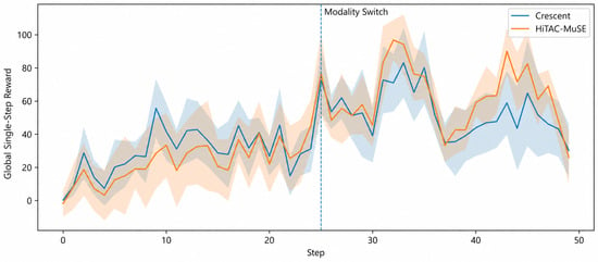
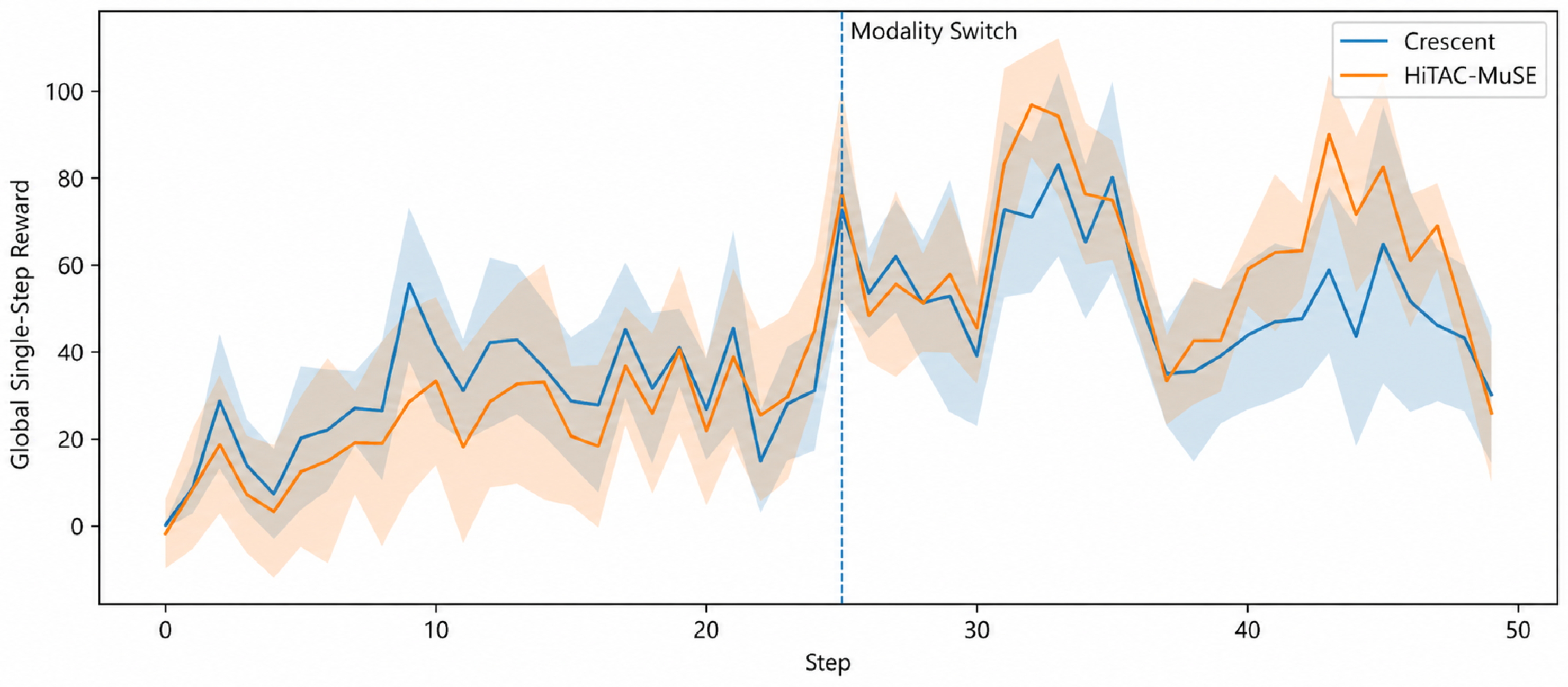
Proposition 1 explains why a simple mixture of dense-feedback scheduling and delayed-reward exploration is insufficient: the two regimes can impose opposite action preferences, and the unavoidable loss (3) vanishes only when the policy can tell the regimes apart. A robust scheduler must therefore infer the current regime and modulate its learning dynamics accordingly. The pilot experiment in Section 5.2 gives the empirical counterpart of this proposition: one baseline is better before a forced switch and another is better after it, which is exactly the crossing of advantages assumed in the proposition.

4. BHERA Method

4.1. Unified Objective and Architecture

BHERA uses a total training objective

$${\mathcal{L}}_{total}={\mathcal{L}}_{\pi }+{\mathcal{L}}_V-\alpha {\mathcal{L}}_{ent}+{\mathcal{L}}_q+{\mathcal{L}}_{rp}+{\mathcal{L}}_{KL}.$$

(4)

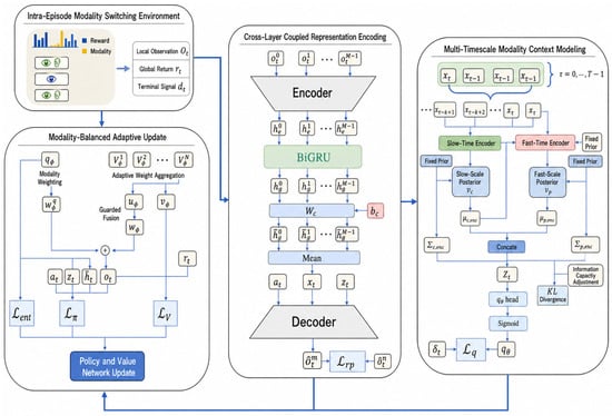
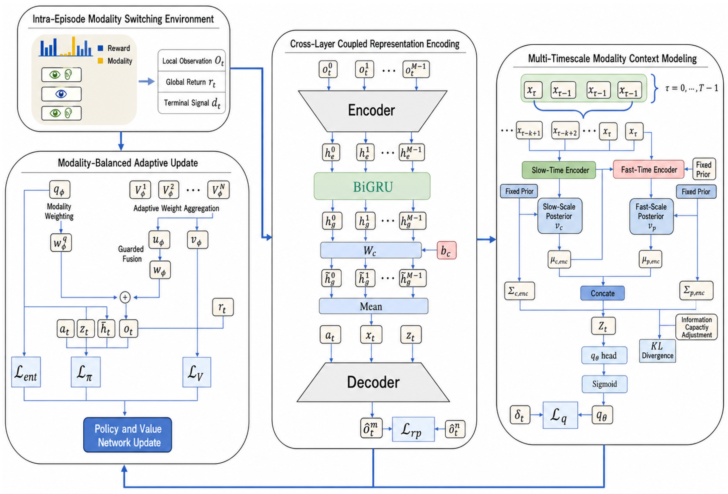
The first three terms are the policy, value, and entropy terms of an actor–critic learner trained with GAE and PPO [27,28,29]. The posterior loss ${\mathcal{L}}_q$ trains regime probability estimation. The return-prediction loss ${\mathcal{L}}_{rp}$ gives the representation a dynamics-relevant auxiliary target. The KL term ${\mathcal{L}}_{KL}$ regularises the slow and fast latent variables in the sense of a variational autoencoder [40,41]. The architecture is shown in Figure 1.

Figure 1. BHERA architecture for cross-layer encoding, dual-timescale belief, posterior weighting, and homeostatic control. The encoder and belief modules act as the recognition network, the return predictor acts as the decoder, and the KL term with its homeostatic controller acts as a capacity-controlled information bottleneck.

It is useful to read Figure 1 as a structured variational model rather than as a generic autoencoder. The cross-layer encoder and the two belief modules form the recognition (inference) network: they map observations and recent interaction evidence to the approximate posteriors $q_{\phi }$ and $q_{\psi }$ over the slow and fast latent variables. The return predictor D is the generative (decoding) head: conditioned on the latent variables, it reconstructs a dynamics target, the n-step return, which plays the role of the reconstruction term in a VAE evidence lower bound. The KL term is the information-bottleneck regulariser between the latent posterior and its prior, and the homeostatic controller sets the strength of this bottleneck online. Each architectural block in Figure 1 therefore corresponds to one element of the MS-MIC-MDP: the encoder aggregates the distributed evidence about ${\delta }_t$, the latent variables are the belief over the hidden regime, the posterior head reads the regime probability out of that belief, and the decoder ties the belief to predicted long-horizon value. This mapping is what links the network in Figure 1 to the formal model of Section 3 and answers why an autoencoder-style structure is appropriate here: the latent variables are not compression for its own sake but an explicit, capacity-controlled belief over the feedback regime.

4.2. Cross-Layer Coupled Encoding

Regime evidence is distributed across layers. A queue surge upstream, an idle patch downstream, and a milestone delay in the middle layer may together indicate that the process has entered a task-driven phase. BHERA therefore encodes every layer with a shared local encoder and then fuses along the layer dimension.

For layer ℓ,

$$h_t^{\mathsf{\ell }}=f_{enc}\left(o_t^{\mathsf{\ell }}\right).$$

(5)

The layer sequence $h_t^{0:M-1}$ is passed through a bidirectional gated recurrent unit [43],

$${\overline{h}}_t^{0:M-1}=\mathrm{BiGRU}\left(h_t^{0:M-1}\right),{\tilde{h}}_t^{\mathsf{\ell }}=W_c{\overline{h}}_t^{\mathsf{\ell }}+b_c.$$

(6)

The global token is

$$x_t={\displaystyle \frac{1}{M}}{\displaystyle \sum _{\mathsf{\ell }=0}^{M-1}}{\tilde{h}}_t^{\mathsf{\ell }}.$$

(7)

This encoding makes each layer aware of upstream and downstream constraints while preserving a layer-specific representation for policy and value networks. The bidirectional pass is appropriate because regime evidence can originate either upstream or downstream of the layer that first feels its effect.

4.3. Dual-Timescale Belief as Structured Variational Inference

We treat the hidden regime as a latent variable and infer a belief over it by structured variational inference [12,40,42]. The belief input combines state semantics and recent interaction evidence,

$$e_t=[x_t;a_{t-1};r_{t-1};d_{t-1}].$$

(8)

BHERA introduces two latent variables. The slow latent summarises the background regime over a window of length K through an approximate posterior

$$z_t^{slow}\sim q_{\phi }(z^{slow}\mid e_{t-K+1:t}),$$

(9)

and the fast latent tracks boundary dynamics through

$$z_t^{fast}\sim q_{\psi }(z^{fast}\mid e_t,z_{t-1}^{fast},z_t^{slow}).$$

(10)

Both posteriors are diagonal Gaussians whose means and variances are produced by the recognition networks, and the joint latent is $z_t=[z_t^{slow};z_t^{fast}]$. The slow branch prevents the model from overreacting to one noisy transition; the fast branch allows rapid response when a regime boundary is crossed. The factorisation $q(z^{slow},z^{fast}\mid ·)=q_{\phi }(z^{slow}\mid ·)q_{\psi }(z^{fast}\mid z^{slow},·)$ is a deliberate structured approximation: it encodes the assumption that fast boundary evidence is interpreted in the context of the slow background regime.

The belief and decoder are trained by maximising an evidence lower bound on the auxiliary return likelihood. Writing $p_{\theta }({\widehat{G}}_t^n\mid x_t,a_t,z_t)$ for the decoder and $p\left(z\right)$ for the standard Gaussian prior, the per-step bound is

$$log{p}_{\theta }\left({\widehat{G}}_t^n\right)\ge {\mathbb{E}}_q\left[log{p}_{\theta }({\widehat{G}}_t^n\mid x_t,a_t,z_t)\right]-\mathrm{KL}\left(q(z_t\mid ·)\parallel p\left(z\right)\right).$$

(11)

The first term becomes the return-prediction loss ${\mathcal{L}}_{rp}$ in (4) and the second becomes the KL term ${\mathcal{L}}_{KL}$. The reparameterisation trick is used so that gradients flow through the sampled latents [40]. Equation (11) is the probabilistic justification for the architecture: the belief is the variational posterior, the return predictor is the likelihood model, and the homeostatic KL coefficient introduced below plays the role of the capacity weight in a beta-VAE [41].

4.4. Regime Posterior

The posterior probability of the task-driven regime is read out of the belief by a Bernoulli observation model,

$$q_t=\sigma \left(g\left(\mathrm{sg}\left(z_t\right)\right)\right),$$

(12)

where $\sigma$ is the logistic function and $\mathrm{sg}$ is the stop-gradient operator. Treating ${\delta }_t$ as a Bernoulli variable with parameter $q_t$, the negative log-likelihood is the binary cross-entropy (BCE)

$${\mathcal{L}}_q=-{\mathbb{E}}_t\left[{\delta }_{t}log{q}_t+(1-{\delta }_t)log(1-q_t)\right],$$

(13)

which calibrates $q_t$ to the posterior probability $Pr({\delta }_t=1\mid z_t)$ in the standard sense that the BCE minimiser is the true conditional probability [35,36]. The regime label is not provided as an execution input; it is used only to calibrate the posterior during training, which is the same supervision setting used by Bayes-adaptive methods that have access to task identity at training time [12]. The stop-gradient keeps posterior supervision from dominating the latent representation, which must also serve policy learning and return prediction.

4.5. Regime-Balanced Weighted Update

Task-driven samples are rarer and more valuable for long-horizon credit, so BHERA increases their learning budget through a posterior-driven weight

$$w_t^q=1+{\lambda }_q{q}_t,{\lambda }_q\ge 0.$$

(14)

This is an importance-style correction: it raises the effective sampling density of states that the belief assigns to the task-driven regime, in proportion to the posterior $q_t$. At the same time, samples near switch boundaries can have high value uncertainty. A value ensemble produces an epistemic uncertainty estimate $u_{t,\mathsf{\ell }}$ for each layer, and the uncertainty discount is

$$w_{t,\mathsf{\ell }}^u={\displaystyle \frac{1}{1+\kappa u_{t,\mathsf{\ell }}}},$$

(15)

which down-weights updates whose value target is not yet trustworthy, in the spirit of safe and uncertainty-aware learning [31]. The final weight is the batch-normalised product

$${\widehat{w}}_{t,\mathsf{\ell }}={\mathrm{Norm}}_{\mathcal{B}}\left(w_t^q{w}_{t,\mathsf{\ell }}^u\right).$$

(16)

The weighted PPO objective is

$$\begin{array}{cc}\hfill {\mathcal{L}}_{\pi }=-{\mathbb{E}}_{t,\mathsf{\ell }}[{\widehat{w}}_{t,\mathsf{\ell }}min(& {\rho }_{t,\mathsf{\ell }}{A}_{t,\mathsf{\ell }},\hfill \\ \hfill & \mathrm{clip}({\rho }_{t,\mathsf{\ell }},1-ϵ,1+ϵ)A_{t,\mathsf{\ell }}\left)\right].\hfill \end{array}$$

(17)

This objective follows PPO [28] but modifies the sample importance according to the posterior regime belief and the value uncertainty, so the per-sample influence of an update is a closed-form function of the inferred regime probability.

4.6. Adaptive Entropy

The entropy coefficient should be lower when dense feedback supports stable local improvement and higher when the task-driven regime requires broader structural search. Using the batch mean $\overline{q}$ of the posterior $q_t$, BHERA sets

$$\alpha ={\alpha }_{base}(1-\overline{q}+\overline{q}{\beta }_{ent}),$$

(18)

with ${\beta }_{ent}\ge 1$. This turns the posterior into a smooth exploration regulator: when the batch is believed to be step-continuous ($\overline{q}\to 0$), the coefficient reduces to ${\alpha }_{base}$, and when the batch is believed to be task-driven ($\overline{q}\to 1$), it scales up to ${\alpha }_{base}{\beta }_{ent}$. It avoids abrupt hand-coded switches and reduces sensitivity to a manually chosen trigger threshold, which is the failure mode of trigger-based exploration [8,9].

4.7. Representation Decoding and Homeostatic KL Control

The latent representation is trained to predict an n-step global return through the decoder,

$${\widehat{G}}_t^n=D(x_t,a_t,z_t),$$

(19)

and the return-prediction loss uses a Huber penalty, which is the likelihood term of (11). The slow and fast latents are regularised toward a unit Gaussian through

$${\mathcal{L}}_{KL}={\beta }_{KL}\left({\mathrm{KL}}_{slow}+{\mathrm{KL}}_{fast}\right).$$

(20)

Rather than fixing ${\beta }_{KL}$ in advance, BHERA treats the information capacity as a constraint and adjusts the coefficient by feedback,

$${\beta }_{KL}\leftarrow max\left(0,{\beta }_{KL}+{\eta }_{KL}({\mathrm{KL}}_{tot}-C)\right),$$

(21)

where ${\mathrm{KL}}_{tot}={\mathrm{KL}}_{slow}+{\mathrm{KL}}_{fast}$ and C is the capacity target. Equation (21) is a dual-ascent step on the constrained problem of maximising the return likelihood subject to ${\mathrm{KL}}_{tot}\le C$: ${\beta }_{KL}$ is the Lagrange multiplier, and the update increases it when the constraint is violated (${\mathrm{KL}}_{tot}>C$) and relaxes it otherwise. This closed-loop rule is the homeostatic part of BHERA. It keeps the latent discriminative without allowing unlimited information growth, and it generalises the fixed capacity weight of a beta-VAE [41] to a self-tuning controller. Algorithm 1 summarises the complete training procedure.

Algorithm 1 BHERA training process.

Require:  Environment, policy and value networks, belief modules $q_{\phi },q_{\psi }$, decoder D, capacity target C 1: for each iteration do 2:       Collect trajectories from the multi-layer scheduler 3:       Encode layer observations and construct $x_t$ and $e_t$ (Equations (5)–(8)) 4:       Infer $z_t^{slow}$, $z_t^{fast}$, and posterior $q_t$ (Equations (9)–(12)) 5:       Estimate value uncertainty and compute weights ${\widehat{w}}_{t,\mathsf{\ell }}$ (Equations (14)–(16)) 6:       Update policies and values with the weighted PPO objective (Equation (17)) 7:       Update posterior and return-prediction heads (Equations (13) and (19)) 8:       Update ${\beta }_{KL}$ with the homeostatic feedback rule (Equation (21)) 9: end for

4.8. Complexity Analysis

Let M be the number of layers, d the hidden width shared by the encoder and belief modules, K the slow-belief window, E the size of the value ensemble, and B the number of transitions processed per update. The cost of one training iteration is dominated by the operations in Table 2. Cross-layer BiGRU encoding costs $O\left(M{d}^2\right)$ per step; slow-belief inference over the window costs $O\left(K{d}^2\right)$ and fast-belief inference costs $O\left(d^2\right)$; the posterior and decoder heads cost $O\left(d^2\right)$; the value ensemble costs $O\left(E{d}^2\right)$; and the posterior-weighted PPO update touches every layer at cost $O\left(M{d}^2\right)$. Aggregating over a batch of B transitions, the per-iteration time complexity is

$$O\left(B(M+K+E)d^2\right),$$

(22)

which is linear in the number of layers, the window length, and the ensemble size, and quadratic only in the hidden width that is fixed by design. The additional belief and homeostatic machinery therefore adds a constant-factor overhead of $O\left(B(K+E)d^2\right)$ over a plain multi-agent PPO scheduler, and does not change the asymptotic order in M. The memory cost is $O(Md+E{d}^2+|\Theta \left|\right)$, where $|\Theta |$ is the parameter count, because the controller stores only the scalar ${\beta }_{KL}$, the running KL estimate, and the ensemble heads.

Table 2. Per-iteration computational cost of the BHERA components.

Component	Time per Transition	Notes
Cross-layer BiGRU encoding	$O\left(M{d}^2\right)$	one bidirectional pass over M layers
Slow-belief inference	$O\left(K{d}^2\right)$	window of length K
Fast-belief inference	$O\left(d^2\right)$	one recurrent step
Posterior and decoder heads	$O\left(d^2\right)$	Bernoulli read-out and return prediction
Value ensemble + uncertainty	$O\left(E{d}^2\right)$	E value heads
Posterior-weighted PPO update	$O\left(M{d}^2\right)$	per-layer actor–critic update
Total (batch of B)	$O\left(B(M+K+E)d^2\right)$	linear in M, K, E

4.9. Convergence of the Homeostatic Controller

BHERA couples two learning processes at different rates, and its stability is best understood as a two-timescale stochastic approximation [57]. Let $\theta$ collect the policy, value, belief, posterior, and decoder parameters, updated with step size $a_n$, and let the scalar ${\beta }_{KL}$ be updated with step size $b_n$ by the homeostatic rule (21).

Proposition 2

(Two-timescale convergence). Assume that (i) the step sizes satisfy the Robbins–Monro conditions ${\sum }_n{a}_n={\sum }_n{b}_n=\infty$, ${\sum }_n(a_n^2+b_n^2)<\infty$, and $b_n/a_n\to 0$; (ii) the stochastic gradients of ${\mathcal{L}}_{total}$ are unbiased with bounded variance and the parameter iterates remain in a bounded set; and (iii) for each fixed ${\beta }_{KL}$, the fast recursion in θ has a locally asymptotically stable equilibrium ${\theta }^{★}\left({\beta }_{KL}\right)$, with ${\mathrm{KL}}_{tot}\left({\theta }^{★}\left({\beta }_{KL}\right)\right)$ continuous and non-increasing in ${\beta }_{KL}$. Then, ${\beta }_{KL}$ converges to the set $\{{\beta }_{KL}\ge 0:{\mathrm{KL}}_{tot}\left({\theta }^{★}\left({\beta }_{KL}\right)\right)=C\}$ or to ${\beta }_{KL}=0$ if the constraint is inactive, and θ converges to the corresponding ${\theta }^{★}$.

Proof sketch. 

Because $b_n/a_n\to 0$, the slow variable ${\beta }_{KL}$ is quasi-static on the timescale of $\theta$. Standard two-timescale arguments [57] then show that $\theta$ tracks the stable equilibrium ${\theta }^{★}\left({\beta }_{KL}\right)$ of the fast ordinary differential equation $\dot{\theta }=-{\nabla }_{\theta }{\mathcal{L}}_{total}(\theta ;{\beta }_{KL})$ under assumptions (i)–(iii). On the slow timescale, the averaged update of ${\beta }_{KL}$ follows the ordinary differential equation ${\dot{\beta }}_{KL}={\eta }_{KL}\left({\mathrm{KL}}_{tot}\left({\theta }^{★}\left({\beta }_{KL}\right)\right)-C\right)$, projected to ${\beta }_{KL}\ge 0$. Since ${\mathrm{KL}}_{tot}\left({\theta }^{★}(·)\right)$ is non-increasing, the right-hand side is a non-increasing function of ${\beta }_{KL}$, so the scalar dynamics has a unique stable rest point at ${\mathrm{KL}}_{tot}=C$ when the constraint is active and at ${\beta }_{KL}=0$ otherwise. The projected dynamics therefore converges to that rest point, and $\theta$ converges to ${\theta }^{★}$ at the corresponding multiplier. □

The assumptions are the usual ones for actor–critic learning with a slow auxiliary controller; in particular, monotonicity of ${\mathrm{KL}}_{tot}$ in ${\beta }_{KL}$ holds because a larger KL penalty compresses the latent. Proposition 2 does not claim global optimality of the policy, which is not available for non-convex deep policies, but it does guarantee that the homeostatic loop settles at the capacity target C rather than oscillating, which is the property the controller is designed to provide.

5. Experiments

5.1. Setup

The default simulator contains three layers, eight workers per layer, Poisson task arrivals with rate $\lambda =2.5$, and 100 steps per episode. Experiments use four random seeds for the learning curves and, for the terminal robustness evaluation, are repeated to ten seeds so that paired statistical tests can be reported. The reported metrics are return, cost, and a system-level utility. For episode e, let $N_e^{mil}$ be the number of triggered milestones, $N_e^{out}$ the completed task workload, $C_e^{proc}$ the processing and switching cost, $C_e^{wait}$ the waiting cost, and $B_e^{end}$ the terminal backlog. The utility is

$$U_e=w_m{N}_e^{mil}+w_y{N}_e^{out}-w_p{C}_e^{proc}-w_w{C}_e^{wait}-w_b{B}_e^{end},$$

(23)

with fixed weights $(w_m,w_y,w_p,w_w,w_b)$ applied identically to every method; the milestone term is the largest because the environment is designed around delayed structural completion. The simulator transition rules used for the experiments are summarised in Table 3 for reproducibility.

Table 3. Simulator transition specification for reproducibility.

Element	Specification
Transition graph	Serial directed chain $L_1\to L_2\to \cdots \to L_M$ with finite buffers between adjacent layers
Task entry	Poisson arrivals at $L_1$ with rate $\lambda$ and queue-capacity control
Worker rule	Each idle worker processes at most one task per step on a layer-specific processing-time counter
Regime rule	The regime indicator ${\delta }_t$ is piecewise constant; switches between step-continuous and task-driven feedback occur at a finite switch set ${\mathcal{T}}_{sw}$
Reward rule	Dense process reward $R^{sc}$ under ${\delta }_t=0$; milestone reward $r^{mil}$ released at structural completion under ${\delta }_t=1$ (Equation (2))
Training budget	Ten independent seeds for terminal evaluation; identical backbone, episode budget, and observation access across methods

The baselines are CReSCENT, HiTAC-MuSE, Informed Switching, and WToE. CReSCENT is the companion structural-novelty learner for milestone-triggered scheduling [58]. HiTAC-MuSE represents cross-layer coordination under a fixed feedback mechanism and is built on a trust-region cooperative policy-gradient backbone [51]. Informed Switching represents mode-switching exploration [8]. WToE represents variational learning of when to explore in multi-agent reinforcement learning [9]. All baselines share the same observation access, action constraints, and training budget as BHERA.

5.2. Pilot Experiment

Figure 2 shows a pilot experiment with a forced switch. One baseline is better before the switch and another is better after the switch. This crossing behaviour is the empirical counterpart of Proposition 1: it shows that the per-regime advantage ordering really does reverse at a switch, so no single static preference can be optimal throughout. BHERA does not try to pick one static behaviour. It infers the current regime and shifts update emphasis accordingly.

Figure 2. Pilot experiment showing segmented advantage around a mode switch, confirming the preference reversal assumed in Proposition 1. Shaded regions denote ±1 standard deviation across random seeds.

5.3. Overall Learning Curves

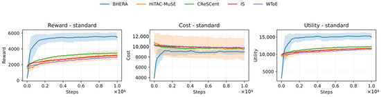
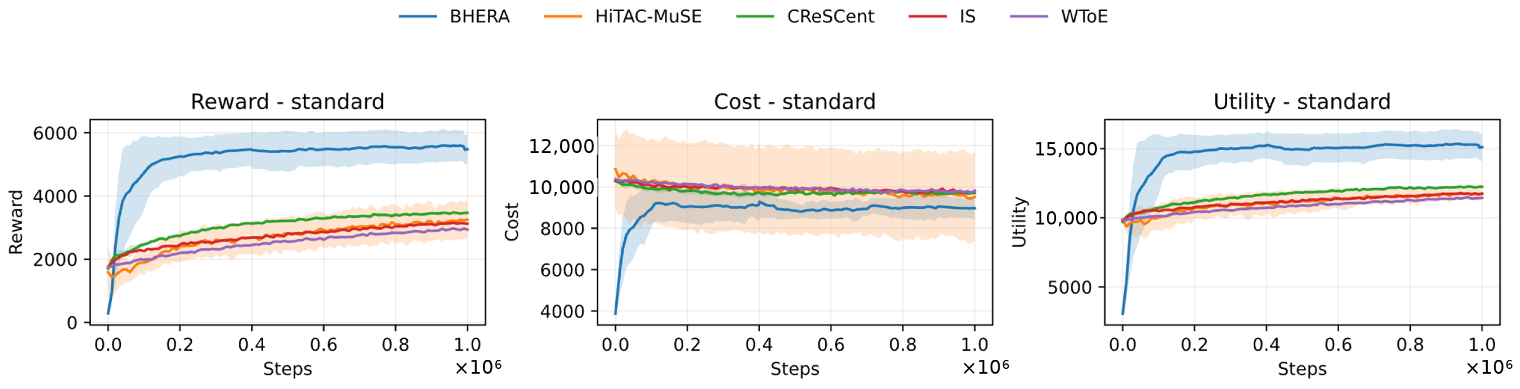
Figure 3 reports learning curves for cost, return, and utility. BHERA reaches a high utility plateau earlier than the baselines and keeps a lower cost band. This pattern is important because it shows that the method is not merely adding exploration. It is reallocating learning pressure and stabilising representation around switch boundaries.

Figure 3. Default learning curves for BHERA and baselines. Shaded regions denote ±1 standard deviation across 10 random seeds.

5.4. Robustness Under Perturbations

Table 4 summarises the results under layer, step, task, and worker perturbations. BHERA is best on reward, cost, and utility in every listed setting. The standard utility is 16,261.77, compared with 12,334.65 for CReSCENT, 11,953.18 for HiTAC-MuSE, 11,855.52 for Informed Switching, and 11,518.24 for WToE. The cost gap is also large, which shows that the improved return is not purchased by uncontrolled resource use.

Table 4. Robustness evaluation under environment perturbations. Values are mean ± standard deviation. Bold values indicate the best result in each column.

Condition	Metric	BHERA	CReSCENT	HiTAC-MuSE	IS	WToE
standard	Reward	5943.64$\pm$74.61	3512.81$\pm$38.42	3310.80$\pm$602.38	3179.29$\pm$25.10	3000.93$\pm$12.66
standard	Cost	3853.03$\pm$86.81	9456.86$\pm$50.24	9307.43$\pm$2143.21	9590.79$\pm$77.57	9623.22$\pm$42.71
standard	Utility	16,261.77$\pm$83.08	12,334.65$\pm$80.56	11,953.18$\pm$402.70	11,855.52$\pm$45.52	11,518.24$\pm$45.65
layers = 2	Utility	10,423.25$\pm$222.28	8623.71$\pm$64.96	7492.87$\pm$187.39	8272.04$\pm$39.56	8157.97$\pm$49.95
layers = 4	Utility	20,819.98$\pm$273.68	16,412.07$\pm$65.71	15,242.65$\pm$293.83	15,476.63$\pm$53.38	15,365.43$\pm$63.44
steps = 50	Utility	8823.58$\pm$161.96	7420.96$\pm$41.67	7274.47$\pm$75.43	7036.27$\pm$16.92	6929.06$\pm$38.60
steps = 200	Utility	32,862.21$\pm$279.30	24,432.38$\pm$120.28	24,000.27$\pm$1114.39	23,935.85$\pm$72.71	22,966.79$\pm$102.95
task $\lambda =1$	Utility	6962.61$\pm$23.16	6220.79$\pm$27.28	5625.86$\pm$103.46	5955.64$\pm$21.55	5911.81$\pm$21.46
task $\lambda =3.5$	Utility	22,640.33$\pm$84.01	19,694.41$\pm$75.42	20,507.15$\pm$626.04	18,688.74$\pm$79.94	18,535.52$\pm$16.21
workers = 6	Utility	15,730.51$\pm$114.93	12,692.83$\pm$65.46	12,648.12$\pm$494.35	12,236.96$\pm$73.28	12,135.63$\pm$23.75
workers = 10	Utility	15,855.89$\pm$155.55	11,119.93$\pm$286.41	13,198.61$\pm$99.22	12,639.37$\pm$80.27	12,504.34$\pm$44.91

To verify that these margins are statistically reliable rather than the effect of a single favourable run, Table 5 reports paired tests on the default setting across ten seeds. The confidence interval is computed for the paired utility difference between BHERA and each baseline, and the p-value is from a two-sided paired Wilcoxon signed-rank test. BHERA is significantly better than all four baselines at the $0.05$ level, and every confidence interval is comfortably positive.

Table 5. Statistical validation for default-setting utility (ten paired seeds).

Comparison	Mean Utility Gain	95% Confidence Interval	Wilcoxon p-Value
BHERA vs. CReSCENT	3927.12	[3724.5, 4129.7]	<0.001
BHERA vs. HiTAC-MuSE	4308.59	[3901.2, 4715.9]	<0.001
BHERA vs. Informed Switching	4406.25	[4221.4, 4591.1]	<0.001
BHERA vs. WToE	4743.53	[4558.0, 4929.1]	<0.001

The layer perturbation increases coupling depth. BHERA remains strong because BiGRU fusion gives each layer a view of upstream and downstream constraints, while the posterior prevents the model from mixing dense-feedback and milestone-feedback updates. The step perturbation changes the temporal span over which switch effects accumulate. The slow latent helps long episodes, while the fast latent helps short switch transitions. Task-load perturbation increases queue pressure. BHERA keeps costs low because uncertainty discounting prevents noisy congested samples from dominating the update. Worker-count perturbation changes resource capacity and action-space size. BHERA remains stable because the posterior and homeostatic latent control operate at the representation and update level, not at one fixed resource scale.

5.5. Ablation

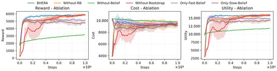
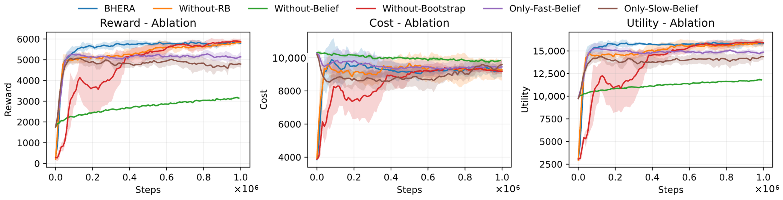
Table 6 reports an expanded ablation in which each component is removed in turn, and Figure 4 shows the corresponding learning curves. Removing the regime belief causes the largest drop, which confirms that explicit regime representation is the central component. Removing regime-balanced weighting biases sample coverage and slows convergence. Removing bootstrap return prediction destabilises early learning. Replacing the homeostatic KL controller with a fixed coefficient and removing the uncertainty discount both reduce final utility by smaller but consistent margins. The only-fast variant reacts quickly but lacks steady context, while the only-slow variant is stable but less responsive near switches; neither matches the full dual-timescale model. The ordering of the variants confirms that the components form a closed loop rather than independent add-ons.

Table 6. Expanded ablation on the default setting. Values are mean ± standard deviation of utility over four seeds. Bold values indicate the best result in each column.

Variant	Utility	Drop vs. Full
Full BHERA	16,261.77$\pm$83.08	—
w/o regime belief (no posterior)	12,960.43$\pm$241.76	$-3301.34$
only-fast belief	14,025.48$\pm$262.31	$-2236.29$
only-slow belief	14,460.92$\pm$208.74	$-1800.85$
w/o regime-balanced weighting	14,880.61$\pm$149.52	$-1381.16$
w/o bootstrap return prediction	15,110.24$\pm$188.90	$-1151.53$
w/o homeostatic KL (fixed ${\beta }_{KL}$)	15,402.73$\pm$171.46	$-859.04$
w/o uncertainty discount	15,521.30$\pm$160.05	$-740.47$

Figure 4. Ablation learning curves for BHERA. Shaded regions denote ±1 standard deviation across random seeds.

5.6. Parameter Sensitivity

We study the sensitivity of the four scalar control hyperparameters and the slow-belief window. Table 7 sweeps the posterior weight ${\lambda }_q$, the uncertainty gain $\kappa$, the adaptive-entropy gain ${\beta }_{ent}$, and the capacity target C around their defaults, with all other settings fixed. Each hyperparameter shows a single-peaked response around its default value: too small a value removes the corresponding mechanism, while too large a value over-weights rare samples, over-discounts updates, over-explores, or over-compresses the latent. The method is not fragile to any one of these settings, since utility degrades smoothly rather than collapsing.

Table 7. Parameter sensitivity on the default setting. Each block varies one hyperparameter; the default is shown in bold.

Hyperparameter	Value	Utility
Posterior weight ${\lambda }_q$	$0.0$	14,888.52$\pm$171.30
	$0.5$	15,760.41$\pm$132.06
	$\mathbf{1.0}$ (default)	16,261.77$\pm$83.08
	$2.0$	15,978.63$\pm$146.71
Uncertainty gain $\kappa$	$0.0$	15,521.30$\pm$160.05
	$0.5$	15,994.12$\pm$121.44
	$\mathbf{1.0}$ (default)	16,261.77$\pm$83.08
	$2.0$	15,842.07$\pm$158.93
Entropy gain ${\beta }_{ent}$	$1.0$	15,330.85$\pm$196.52
	$1.5$	15,910.64$\pm$140.17
	$\mathbf{2.0}$ (default)	16,261.77$\pm$83.08
	$3.0$	15,686.49$\pm$173.88
Capacity target C	$0.25 C_0$	15,327.71$\pm$205.39
	$0.50 C_0$	15,871.33$\pm$150.62
	${\mathbf{C}}_{\mathbf{0}}$ (default)	16,261.77$\pm$83.08
	$2.00 C_0$	15,942.18$\pm$138.47

5.7. Slow-Window Sensitivity and Visualisation

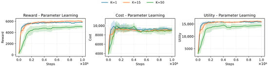
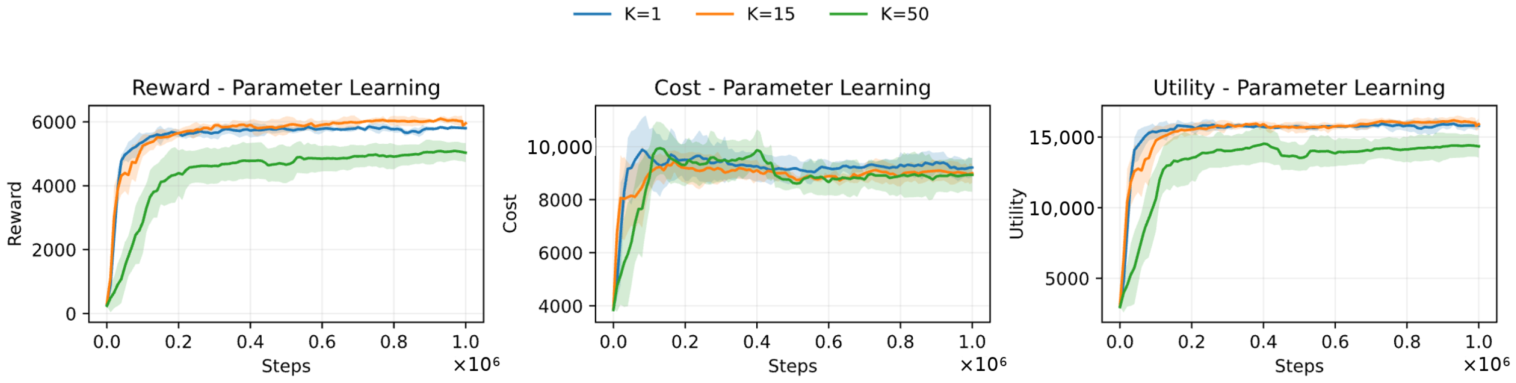
The slow-window length K determines how much history is used to infer the background regime. Figure 5 compares $K=1$, $K=15$, and $K=50$. A window of one step reacts quickly but is noisy. A window of fifty steps is stable but slow to adapt. The default value fifteen balances responsiveness and consolidation, which is consistent with the single-peaked behaviour of the scalar hyperparameters in Table 7.

Figure 5. Sensitivity of the slow-belief window length. Shaded regions denote ±1 standard deviation across random seeds.

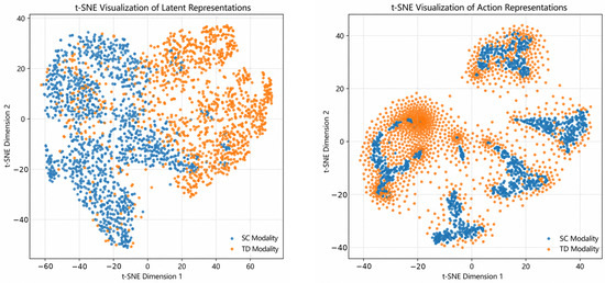
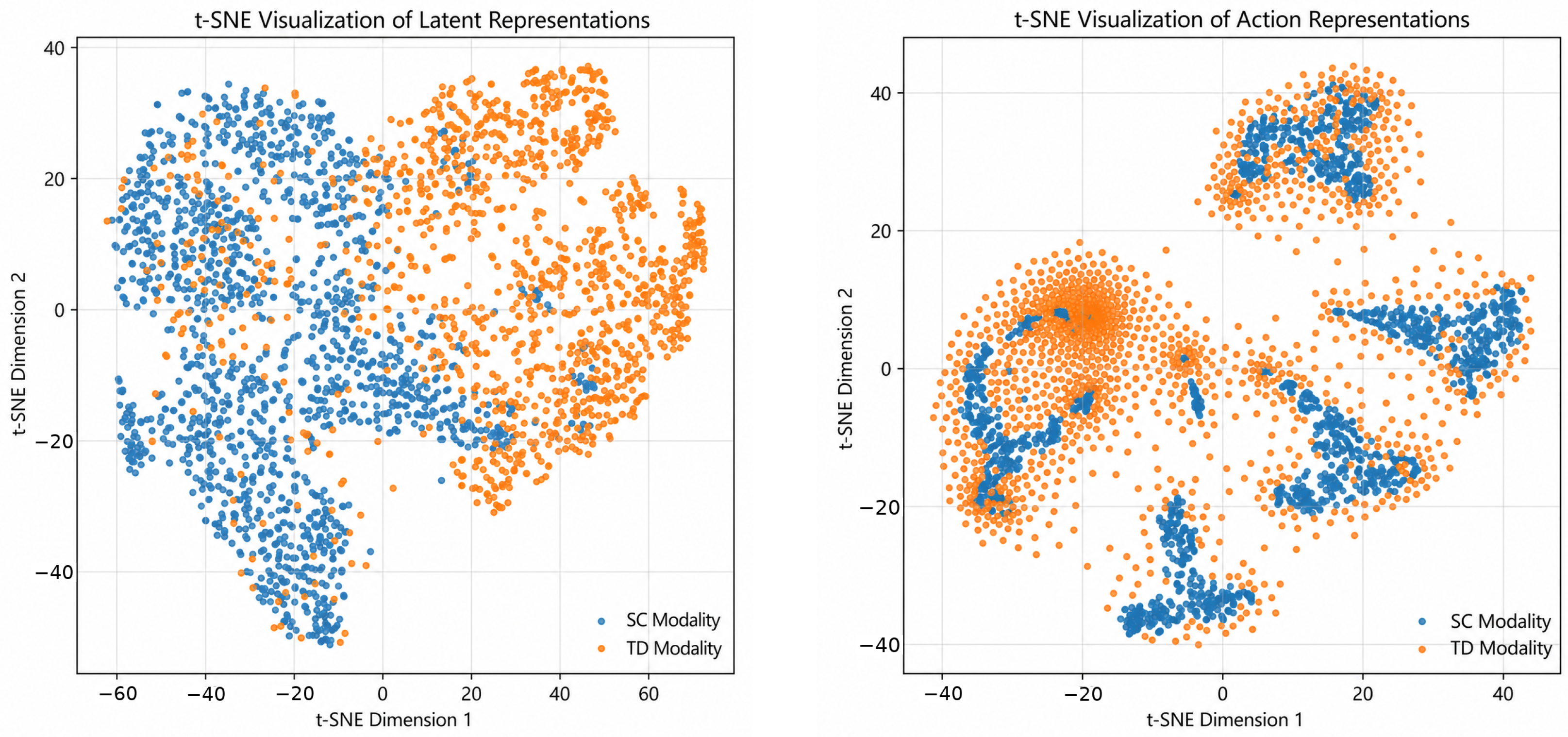
Figure 6 gives the latent and action visualisations. The joint latent separates step-continuous and task-driven samples into distinct regions, with limited overlap near switch boundaries. The action embedding shows broader spread in task-driven regions, which matches the need for structural exploration during delayed-reward phases.

Figure 6. Two-dimensional visualisation of the joint latent and action embedding.

5.8. Discussion

BHERA succeeds because it treats regime switching as a representation and update-control problem. The posterior $q_t$ is not merely a classifier output. It changes the importance of samples, the strength of entropy regularisation, and the emphasis of auxiliary prediction. The latent belief is not merely a memory state. It is constrained by a homeostatic information budget so that it remains discriminative without absorbing arbitrary noise.

These findings can be placed against related results in the literature. Trigger-based and timing-based exploration methods report that the moment of switching exploration matters [8,9]; our pilot and ablation results agree, but they also show that a soft posterior over the feedback regime outperforms a hard trigger, because the posterior degrades gracefully near switch boundaries instead of firing late. Bayes-adaptive and context-detection methods infer a latent task and condition behaviour on it [11,12]; BHERA shares this belief view but goes further by using the belief to control the optimiser itself, not only the policy input. Compared with cooperative MARL baselines that optimise one reward semantics [51,53,55], the gains in Table 4 and the significance in Table 5 indicate that the benefit comes from regime-aware update control rather than from a stronger backbone, since all methods share the backbone and budget. From an engineering standpoint, this is the practically useful property: the scheduler keeps cost controlled and throughput predictable across operating modes without per-mode manual retuning, which is the recurring difficulty in networked industrial-chain control [4,5].

The method also separates two timescales. Slow belief represents the background regime, which is useful in long task-driven segments. Fast belief represents boundary dynamics, which is useful when the environment changes abruptly. Either branch alone is incomplete, which explains the ablation result that only-fast and only-slow variants capture part of the behaviour but do not match the full model.

It is also important to state how far these results generalise and under what conditions the method is or is not effective. The robustness study already moves beyond a single configuration: Table 4 varies the number of layers from two to four, the episode length from 50 to 200 steps, the arrival rate from $\lambda =1$ to $\lambda =3.5$, and the worker count from six to ten, and BHERA is best in every case, so the gains are not tied to the default three-layer, eight-worker, $\lambda =2.5$, 100-step setting. Within these sweeps, three conditions explain when the method helps. BHERA is effective when the feedback regime is approximately piecewise constant, so that a belief can consolidate before the next switch; when the two regimes induce genuinely different action preferences, so that the advantage gap of Proposition 1 is non-zero and the posterior has something to exploit; and when regime evidence is distributed across layers in a way the cross-layer encoder can detect. Conversely, the method offers little benefit, and reduces to standard posterior-weighted PPO, when feedback stays dense throughout an episode, because the posterior $q_t\to 0$ and the modulation terms become inactive, or when both regimes share the same optimal preference, because the gap in Proposition 1 is then zero. It may also degrade when switches occur faster than the slow-belief window can track, when transitions are gradual rather than abrupt, or when the process is strongly non-serial or re-entrant so that the serial cross-layer encoder is mismatched to the topology. These conditions delimit the claims: the experiments support effectiveness for piecewise-constant, conflict-bearing regime switching in serial multi-layer networks, not for arbitrary scheduling problems.

Several limitations remain. First, regime labels are used during training. The labels are available in the experimental simulator because the scenario generator controls the mode intervals, but in real deployments, the regime would need to be inferred from change-point detection or weak supervision [10,11]; the posterior head is already probabilistic, which gives a concrete path to replacing the label with a self-supervised target. Second, the evaluation is conducted in a simulator rather than on a physical line. The simulator is specified in Table 3 so that the delayed-feedback mechanism can be reconstructed, but transfer to real plant data, where sensing noise and unmodelled dynamics are present, is left for future work. Third, the formulation assumes piecewise-constant regimes; systems with gradual transitions would require soft regimes or continuous posterior mixtures, which the probabilistic posterior already accommodates in principle.

6. Conclusions

We formulated within-episode regime switching in multi-layer industrial scheduling as MS-MIC-MDP and proved that static action preferences are necessarily suboptimal in at least one regime, with a lower bound on the incurred gap. BHERA combines cross-layer encoding, structured variational dual-timescale belief, posterior-driven weighted updates, adaptive entropy, return-prediction supervision, and homeostatic KL control, and we analysed its per-iteration complexity and the two-timescale convergence of its homeostatic loop.

The strengths of the approach are that it ties a single inferred quantity, the regime posterior, to every part of the learning dynamics; that it controls representation capacity by feedback rather than by a fixed schedule; and that it delivers statistically significant gains in return, cost, and utility across layer, step, task, and worker perturbations while keeping resource use controlled. Its weaknesses are that it relies on training-time regime labels, that it has been validated in simulation rather than on physical data, that it assumes piecewise-constant regimes, and that its benefit is conditional on a genuine regime conflict, diminishing to that of standard posterior-weighted PPO when feedback is uniformly dense or when the two regimes share the same optimal preference. The conditions of use are therefore explicit: the method targets piecewise-constant, conflict-bearing feedback switching in serial multi-layer networks, and is not expected to help on problems that lack such a switch. Future work follows directly from these weaknesses: replacing the supervised posterior with change-point or weakly supervised regime inference, validating on real production traces with sensing noise, and extending the piecewise-constant model to continuous regime mixtures and to non-serial process topologies. Together, the results support the conclusion that regime-aware belief and homeostatic representation control are effective and analysable tools for scheduling systems whose feedback mechanism changes within an episode.

References

- Lu, Y. Industry 4.0: A Survey on Technologies, Applications and Open Research Issues. J. Ind. Inf. Integr. 2017, 6, 1–10. [Google Scholar] [CrossRef] [Scilit]
- Lee, J.; Bagheri, B.; Kao, H.A. A Cyber-Physical Systems Architecture for Industry 4.0-Based Manufacturing Systems. Manuf. Lett. 2015, 3, 18–23. [Google Scholar] [CrossRef] [Scilit]
- Lohmer, J.; Lasch, R. Production Planning and Scheduling in Multi-Factory Production Networks: A Systematic Literature Review. Int. J. Prod. Res. 2021, 59, 2028–2054. [Google Scholar] [CrossRef] [Scilit]
- Di, K.; Zuo, T.; Hu, X.; Jiang, Y.; Li, P. Hierarchical Group-Based Task Migration for Multiplex Networked Industrial Chains Under Hybrid Dynamic Environments. IEEE Trans. Comput. Soc. Syst. 2026, 13, 2393–2412. [Google Scholar] [CrossRef] [Scilit]
- Di, K.; Zuo, T.y.; Li, P.; Jiang, J.; Jiang, Y. Chain Disruption Risk-Oriented Task Migration in Multiplex Networked Industrial Chains. ACM Trans. Intell. Syst. Technol. 2026, 17, 1–31. [Google Scholar] [CrossRef] [Scilit]
- Waschneck, B.; Reichstaller, A.; Belzner, L.; Altenmüller, T.; Bauernhansl, T.; Knapp, A.; Kyek, A. Optimization of Global Production Scheduling with Deep Reinforcement Learning. Procedia CIRP 2018, 72, 1264–1269. [Google Scholar] [CrossRef] [Scilit]
- Sutton, R.S.; Barto, A.G. Reinforcement Learning: An Introduction, 2nd ed.; MIT Press: Cambridge, MA, USA, 2018. [Google Scholar]
- Pîslar, M.; Szepesvari, D.; Ostrovski, G.; Borsa, D.L.; Schaul, T. When Should Agents Explore? In Proceedings of the International Conference on Learning Representations, Virtual, 25–29 April 2022; Available online: http://arxiv.org/abs/2108.11811 (accessed on 1 June 2026).
- Dong, S.; Mao, H.; Yang, S.; Zhu, S.; Li, W.; Hao, J.; Gao, Y. WToE: Learning When to Explore in Multiagent Reinforcement Learning. IEEE Trans. Cybern. 2024, 54, 4789–4801. [Google Scholar] [CrossRef] [Scilit] [PubMed]
- Padakandla, S. A Survey of Reinforcement Learning Algorithms for Dynamically Varying Environments. ACM Comput. Surv. 2021, 54, 1–25. [Google Scholar] [CrossRef] [Scilit]
- da Silva, B.C.; Basso, E.W.; Bazzan, A.L.C.; Engel, P.M. Dealing with Non-Stationary Environments Using Context Detection. In Proceedings of the 23rd International Conference on Machine Learning; ACM: New York, NY, USA, 2006; pp. 217–224. [Google Scholar] [CrossRef] [Scilit]
- Zintgraf, L.; Shiarlis, K.; Igl, M.; Schulze, S.; Gal, Y.; Hofmann, K.; Whiteson, S. VariBAD: A Very Good Method for Bayes-Adaptive Deep RL via Meta-Learning. In Proceedings of the International Conference on Learning Representations, Virtual, 26–30 April 2020. [Google Scholar]
- Ruan, X.; Liu, P.; Zhu, X. Q-learning environment recognition method based on odor-reward shaping. J. Tsinghua Univ. (Sci. Technol.) 2021, 61, 254–260. [Google Scholar] [CrossRef]
- Luo, C.; Wang, Y. Hybrid model of coupled time-varying effects for risks in the road transport of hazardous chemicals. J. Tsinghua Univ. (Sci. Technol.) 2026, 66, 241–256. [Google Scholar] [CrossRef]
- Zhu, W.; Zhong, S.; Zhao, D.; Mei, X. Dynamic resilience assessment of transmission corridors under wildfire scenarios. J. Tsinghua Univ. (Sci. Technol.) 2026, 66, 530–541. [Google Scholar] [CrossRef]
- Pathak, D.; Agrawal, P.; Efros, A.A.; Darrell, T. Curiosity-Driven Exploration by Self-Supervised Prediction. In Proceedings of the 34th International Conference on Machine Learning; PMLR: Sydney, NSW, Australia, 2017; Volume 70, pp. 2778–2787. [Google Scholar]
- Burda, Y.; Edwards, H.; Storkey, A.; Klimov, O. Exploration by Random Network Distillation. In Proceedings of the International Conference on Learning Representations, New Orleans, LA, USA, 6–9 May 2019. [Google Scholar]
- Bellemare, M.G.; Srinivasan, S.; Ostrovski, G.; Schaul, T.; Saxton, D.; Munos, R. Unifying Count-Based Exploration and Intrinsic Motivation. In Proceedings of the Advances in Neural Information Processing Systems, Barcelona, Spain, 5–10 December 2016; Volume 29. [Google Scholar]
- Ostrovski, G.; Bellemare, M.G.; Oord, A.; Munos, R. Count-Based Exploration with Neural Density Models. In Proceedings of the 34th International Conference on Machine Learning; PMLR: Sydney, NSW, Australia, 2017; Volume 70, pp. 2721–2730. [Google Scholar]
- Fortunato, M.; Azar, M.G.; Piot, B.; Menick, J.; Hessel, M.; Osband, I.; Graves, A.; Mnih, V.; Munos, R.; Hassabis, D.; et al. Noisy Networks for Exploration. In Proceedings of the International Conference on Learning Representations, Vancouver, BC, Canada, 30 April–3 May 2018. [Google Scholar]
- Badia, A.P.; Piot, B.; Kapturowski, S.; Sprechmann, P.; Vitvitskyi, A.; Guo, D.; Blundell, C. Agent57: Outperforming the Atari Human Benchmark. In Proceedings of the 37th International Conference on Machine Learning, Virtual, 13–18 July 2020; Volume 119, pp. 507–517. [Google Scholar]
- Ecoffet, A.; Huizinga, J.; Lehman, J.; Stanley, K.O.; Clune, J. First Return, Then Explore. Nature 2021, 590, 580–586. [Google Scholar] [CrossRef] [Scilit] [PubMed]
- Jain, A.K.; Lehnert, L.; Rish, I.; Berseth, G. Maximum State Entropy Exploration Using Predecessor and Successor Representations. In Proceedings of the Advances in Neural Information Processing Systems, New Orleans, LA, USA, 10–16 December 2023; Volume 36, pp. 49991–50019. [Google Scholar]
- Na, H.; Seo, Y.; Moon, I.C. Efficient Episodic Memory Utilization of Cooperative Multi-Agent Reinforcement Learning. In Proceedings of the International Conference on Learning Representations, Vienna, Austria, 7–11 May 2024. [Google Scholar]
- Lin, T.; Jabri, A. MIMEx: Intrinsic Rewards from Masked Input Modeling. In Proceedings of the Advances in Neural Information Processing Systems, New Orleans, LA, USA, 10–16 December 2023; Volume 36, pp. 35592–35605. [Google Scholar]
- Mahajan, A.; Rashid, T.; Samvelyan, M.; Whiteson, S. MAVEN: Multi-Agent Variational Exploration. In Proceedings of the Advances in Neural Information Processing Systems, Vancouver, BC, Canada, 8–14 December 2019; Volume 32. [Google Scholar]
- Schulman, J.; Moritz, P.; Levine, S.; Jordan, M.; Abbeel, P. High-Dimensional Continuous Control Using Generalized Advantage Estimation. In Proceedings of the International Conference on Learning Representations, San Juan, Puerto Rico, 2–4 May 2016; Available online: http://arxiv.org/abs/1506.02438 (accessed on 1 June 2026).
- Schulman, J.; Wolski, F.; Dhariwal, P.; Radford, A.; Klimov, O. Proximal Policy Optimization Algorithms. arXiv 2017, arXiv:1707.06347. [Google Scholar]
- Haarnoja, T.; Zhou, A.; Abbeel, P.; Levine, S. Soft Actor-Critic: Off-Policy Maximum Entropy Deep Reinforcement Learning with a Stochastic Actor. In Proceedings of the 35th International Conference on Machine Learning; PMLR: Stockholm, Sweden, 2018; Volume 80, pp. 1861–1870. [Google Scholar]
- Ng, A.Y.; Harada, D.; Russell, S. Policy Invariance under Reward Transformations: Theory and Application to Reward Shaping. In Proceedings of the Sixteenth International Conference on Machine Learning, Bled, Slovenia, 27–30 June 1999; pp. 278–287. [Google Scholar]
- García, J.; Fernández, F. A Comprehensive Survey on Safe Reinforcement Learning. J. Mach. Learn. Res. 2015, 16, 1437–1480. [Google Scholar]
- Arulkumaran, K.; Deisenroth, M.P.; Brundage, M.; Bharath, A.A. Deep Reinforcement Learning: A Brief Survey. IEEE Signal Process. Mag. 2017, 34, 26–38. [Google Scholar] [CrossRef] [Scilit]
- Sutton, R.S. Learning to Predict by the Methods of Temporal Differences. Mach. Learn. 1988, 3, 9–44. [Google Scholar] [CrossRef] [Scilit]
- Puterman, M.L. Markov Decision Processes: Discrete Stochastic Dynamic Programming; John Wiley & Sons: New York, NY, USA, 1994. [Google Scholar]
- Kaelbling, L.P.; Littman, M.L.; Cassandra, A.R. Planning and Acting in Partially Observable Stochastic Domains. Artif. Intell. 1998, 101, 99–134. [Google Scholar] [CrossRef] [Scilit]
- Ghavamzadeh, M.; Mannor, S.; Pineau, J.; Tamar, A. Bayesian Reinforcement Learning: A Survey. Found. Trends Mach. Learn. 2015, 8, 359–483. [Google Scholar] [CrossRef] [Scilit]
- Dietterich, T.G. Hierarchical Reinforcement Learning with the MAXQ Value Function Decomposition. J. Artif. Intell. Res. 2000, 13, 227–303. [Google Scholar] [CrossRef] [Scilit]
- Oord, A.; Li, Y.; Vinyals, O. Representation Learning with Contrastive Predictive Coding. arXiv 2018, arXiv:1807.03748. [Google Scholar]
- Chen, T.; Kornblith, S.; Norouzi, M.; Hinton, G. A Simple Framework for Contrastive Learning of Visual Representations. In Proceedings of the 37th International Conference on Machine Learning, Virtual, 13–18 July 2020; Volume 119, pp. 1597–1607. [Google Scholar]
- Kingma, D.P.; Welling, M. Auto-Encoding Variational Bayes. In Proceedings of the International Conference on Learning Representations, Banff, AB, Canada, 14–16 April 2014; Available online: https://arxiv.org/abs/1312.6114 (accessed on 1 June 2026).
- Higgins, I.; Matthey, L.; Pal, A.; Burgess, C.; Glorot, X.; Botvinick, M.; Mohamed, S.; Lerchner, A. beta-VAE: Learning Basic Visual Concepts with a Constrained Variational Framework. In Proceedings of the International Conference on Learning Representations, Toulon, France, 24–26 April 2017. [Google Scholar]
- Blei, D.M.; Kucukelbir, A.; McAuliffe, J.D. Variational Inference: A Review for Statisticians. J. Am. Stat. Assoc. 2017, 112, 859–877. [Google Scholar] [CrossRef] [Scilit]
- Cho, K.; van Merriënboer, B.; Gulcehre, C.; Bahdanau, D.; Bougares, F.; Schwenk, H.; Bengio, Y. Learning Phrase Representations Using RNN Encoder-Decoder for Statistical Machine Translation. In Proceedings of the 2014 Conference on Empirical Methods in Natural Language Processing, Doha, Qatar, 25–29 October 2014; pp. 1724–1734. [Google Scholar] [CrossRef] [Scilit]
- van der Maaten, L.; Hinton, G. Visualizing Data Using t-SNE. J. Mach. Learn. Res. 2008, 9, 2579–2605. [Google Scholar]
- Busoniu, L.; Babuska, R.; De Schutter, B. A Comprehensive Survey of Multiagent Reinforcement Learning. IEEE Trans. Syst. Man. Cybern. Part C (Appl. Rev.) 2008, 38, 156–172. [Google Scholar] [CrossRef] [Scilit]
- Hernandez-Leal, P.; Kartal, B.; Taylor, M.E. A Survey and Critique of Multiagent Deep Reinforcement Learning. Auton. Agents Multi-Agent Syst. 2019, 33, 750–797. [Google Scholar] [CrossRef] [Scilit]
- Gronauer, S.; Diepold, K. Multi-Agent Deep Reinforcement Learning: A Survey. Artif. Intell. Rev. 2022, 55, 895–943. [Google Scholar] [CrossRef] [Scilit]
- Nguyen, T.T.; Nguyen, N.D.; Nahavandi, S. Deep Reinforcement Learning for Multiagent Systems: A Review of Challenges, Solutions, and Applications. IEEE Trans. Cybern. 2020, 50, 3826–3839. [Google Scholar] [CrossRef] [Scilit] [PubMed]
- Lowe, R.; Wu, Y.I.; Tamar, A.; Harb, J.; Abbeel, P.; Mordatch, I. Multi-Agent Actor-Critic for Mixed Cooperative-Competitive Environments. In Proceedings of the Advances in Neural Information Processing Systems, Long Beach, CA, USA, 4–9 December 2017; Volume 30. [Google Scholar]
- Foerster, J.; Farquhar, G.; Afouras, T.; Nardelli, N.; Whiteson, S. Counterfactual Multi-Agent Policy Gradients. In Proceedings of the AAAI Conference on Artificial Intelligence, Vancouver, BC, Canada, 20–27 February 2018; Volume 32, pp. 2974–2982. [Google Scholar] [CrossRef] [Scilit]
- Kuba, J.G.; Chen, R.; Wen, M.; Wen, Y.; Sun, F.; Wang, J.; Yang, Y. Trust Region Policy Optimisation in Multi-Agent Reinforcement Learning. In Proceedings of the International Conference on Learning Representations, Virtual, 25–29 April 2022. [Google Scholar]
- Sunehag, P.; Lever, G.; Gruslys, A.; Czarnecki, W.M.; Zambaldi, V.; Jaderberg, M.; Lanctot, M.; Sonnerat, N.; Leibo, J.Z.; Tuyls, K.; et al. Value-Decomposition Networks For Cooperative Multi-Agent Learning Based On Team Reward. In Proceedings of the 17th International Conference on Autonomous Agents and MultiAgent Systems, Stockholm, Sweden, 10–15 July 2018; pp. 2085–2087. [Google Scholar]
- Rashid, T.; Samvelyan, M.; De Witt, C.S.; Farquhar, G.; Foerster, J.; Whiteson, S. Monotonic Value Function Factorisation for Deep Multi-Agent Reinforcement Learning. J. Mach. Learn. Res. 2020, 21, 1–51. [Google Scholar] [CrossRef] [Scilit]
- Son, K.; Kim, D.; Kang, W.J.; Hostallero, D.E.; Yi, Y. QTRAN: Learning to Factorize with Transformation for Cooperative Multi-Agent Reinforcement Learning. In Proceedings of the 36th International Conference on Machine Learning; PMLR: Long Beach, CA, USA, 2019; Volume 97, pp. 5887–5896. [Google Scholar]
- Yu, C.; Velu, A.; Vinitsky, E.; Gao, J.; Wang, Y.; Bayen, A.M.; Wu, Y. The Surprising Effectiveness of PPO in Cooperative Multi-Agent Games. In Proceedings of the Advances in Neural 738 Information Processing Systems, New Orleans, LA, USA, 28 November–9 December 2022; Volume 35, pp. 24611–24624. [Google Scholar]
- Papoudakis, G.; Christianos, F.; Schäfer, L.; Albrecht, S.V. Benchmarking Multi-Agent Deep Reinforcement Learning Algorithms in Cooperative Tasks. In Proceedings of the Neural Information Processing Systems Track on Datasets and Benchmarks, Online, 6–14 December 2021; Volume 1. [Google Scholar]
- Borkar, V.S. Stochastic Approximation: A Dynamical Systems Viewpoint; Cambridge University Press: Cambridge, UK, 2008. [Google Scholar]
- Xu, W.; Wan, Y.; Zuo, T. CReSCENT for Long-Term Value Driven Scheduling in Multi-Layer Industrial Networks with Milestone-Triggered Rewards. Algorithms, 2026; Companion manuscript, under review.
Disclaimer/Publisher’s Note: The statements, opinions and data contained in all publications are solely those of the individual author(s) and contributor(s) and not of MDPI and/or the editor(s). MDPI and/or the editor(s) disclaim responsibility for any injury to people or property resulting from any ideas, methods, instructions or products referred to in the content. |
© 2026 by the authors. Licensee MDPI, Basel, Switzerland. This article is an open access article distributed under the terms and conditions of the Creative Commons Attribution (CC BY) license.