


Abstract
Efficient Distributed Computing is still a major challenge, especially in networks composed of very-low-resource embedded systems, e.g., tiny microcontrollers deployed in sensor networks. This work will, firstly, address the design and implementation of event-driven and real-time capable low-resource Virtual Machines (VMs) tightly coupled to communication-centric systems, and secondly, address messaging and routing in mesh-grid networks. The distributed VM network herein forms one big virtual computer executing typically the same program on each node, but processing different data with different control states. The VM provides an integrated program code compiler and an optimized Bytecode processor. The programming language of the VM supports channel-based communication, multi-tasking, and event-based (asynchronous) data processing following the CSP model. The VM fits in microcontrollers with only a few kB of RAM and ROM. A major part of this work is dedicated to network messaging (supported by the VM, too) and routing in two-dimensional mesh-grid networks with a varying degree k of communication ports per node (connectivity degree k), and especially considering the odd but technical relevant case, k = 3, which introduces challenges in message routing that are solved herein. This study demonstrates the performance and suitability of our VM approach for distributed sensor networks performing distributed Machine Learning and clustering by using local sensor data only.
1. Introduction
With increasing node density in sensor networks, there is a shift in the sensor network paradigm towards coupling data processing tightly to sensors, i.e., enabling in-sensor processing and direct sensor–sensor communication. Sensor networks can communicate wirelessly or wired, as summarized by Fammini et al. [1]. In industrial contexts, there are primarily wired networks based on Ethernet technologies and wireless communication based on industrial WLAN. Sensor networks can be considered theoretically as distributed graphs of computational nodes capable to communicate with neighbor nodes. One major network graph topology is the two-dimensional mesh grid. The operational stability of single sensors, as well as composed sensor networks, can be compromised by environmental factors (e.g., power supply, electrical interference, outdoor conditions, and many more), other external devices, hardware noise, improper measurement techniques, and cyber-attacks. These factors can cause data inconsistency and serious communication issues. Distributed algorithms, e.g., distributed consent about the correctness of sensor readings as discussed by Kenyeres et al. [2], require a suitable and efficient communication architecture and communication protocol. If we assume that all nodes have different asynchronous clocks, the communication protocol should provide low latency, low jitter, and optionally auxiliary hardware signals for clock synchronization in the network.
In addition to the operational expressiveness of the data processing system, there is a requirement for programmability of sensors, either on a binary-encoded program (native machine or abstract instructions) or on a textual programming language level [3,4]. The sensor network architecture and the communication system must be scalable towards thousands of interacting sensor nodes, and it is important that data processing, communication, and protocols are considered together. A sensor network can be heterogeneous, i.e., with repent to different hardware architectures, memory and energy resources, and peripherals. Even in homogeneous networks, there is a requirement for hardware layer abstraction for data processing and communication, including compilers. Virtual Machine architectures are commonly deployed on powerful computers. Sensor nodes, especially regarding material-integrated sensor networks, are commonly equipped with very-low-resource embedded systems and microcontrollers. Distributed sensor networks operate commonly under resource constrains, as elaborated by Sadler [5], especially concerning energy constraints. If there are energy constrains, then the computational power of a sensor will be strictly limited, too. Implementing VMs on such low-resource systems is a challenge. For example, the Google V8-based node.js platform requires more than 10 MB of RAM (on startup) and 20 MB of ROM code storage (based on own measurements, see also [6,7]), which are neither suitable nor scalable for any tiny microcontroller. Even Hong [8], with their TinyVM and application-specific synthesis of a VM (from source code) and code compression, reports higher resource usage than that addressed in our work. VMs can be classified into register- and stack-centric processors, as discussed and compared by Šimek et al. [9], but with a focus on Just-in-Time compilation (of machine code, which is not addressed in this work for resource reasons). Stack-based machines offer advanced and simplified compilation of program code, e.g., proven with the REXA-VM [10], by bypassing register allocation phases. Marques et al. demonstrated the deployment of a 32-bit register-based VM in wireless sensor networks on top of the TinyOS [11]. Most modern VMs are mixed architectures. It is always difficult to determine the lower bound of resources (RAM, ROM). Levis et al. [12] introduced the Mate VM on top of the TinyOS, and reported the deployment on low- and very-low-resource microcontrollers (typically 8–128 kB RAM). They demonstrated the VM implementation under 1 kB RAM and 16 kB ROM constraints. Some concepts from Mate, like event-driven and communication-centric programming, influenced the PLX VM architecture introduced in this work, but with a focus on grid computing, which other VMs do not support at the first level.
However, all these VMs do not provide event-based processing; multi-tasking and synchronization capabilities and extensive networking support are aligned to mesh-grid networks with distributed computing—all together, as required by the system, e.g., by sensor networks performing distributed Structural Health Monitoring (SHM). Simple VMs like Mate provide only generic or low-level communication features with limited routing capabilities. The PLX VM provides channel-based communication operations with a high level of expressiveness and advanced message routing, which are fitted tightly to grid-based distributed computing in sensor networks. Finally, we can classify VM architectures into monolithic and non-monolithic systems with respect to the integration of a source-code compiler, i.e., providing a text or binary code interface. Binary VMs are difficult to handle in heterogeneous systems, e.g., if there are multiple ISA versions within a network. Therefore, programming a VM with a fault-tolerant source code text interface is required. Most relevant work addresses wireless sensor networks. Wired networks can be required in specific sensing applications, e.g., material-integrated sensor networks, where wireless (radio- or light-based) communication is not possible. Additionally, wired communication can provide power transfer, too, and finally support advanced distributed computing, e.g., by using the Cellular Automata (CA) paradigm, such as that applied to image processing by Rosin et al. [13].
Machine Learning (ML) is used to predict features of systems from data, typically split into parameterizable models and algorithms, used for prediction and training of the model. Distributed sensor networks should optimally process sensor data locally, including ML. Distributed computing requires advanced, efficient, and reliable communication among nodes, as discussed by Seng et al. [14] for distributed ML in the Internet of Things (IoT), where the communication layer is the middleware between the application and sensing layer, as well as crucial for inter-node data exchange. Distributed clustering as a common method for spatial data fusion requires efficient communication, too, as discussed by Taherkordi et al. [15].
A distributed sensor network (DSN) is basically a set of k connected nodes N, connected by l edges E:
The edges primarily provide communication links, which can be unidirectional, bidirectional, or pairwise unidirectional. The communication provides data transfer as well as synchronization between nodes. For SHM and GUW measurements, the computational power of each node, as well as the communication latency (between nodes or along a network path), sets operational constraints and affects the precision or accuracy of measuring methods, and finally, the precision of predictive models. Optionally, the edge nodes can also be used to supply energy, permanently or temporarily, by using the existing communication wires for energy distribution in the network (electrical wires as well as optical fibers, e.g., demonstrated by Budelmann et al. [16]). Each edge is connected to a node via a port p. A node has a fixed number of ports pn.
Typical network architectures, especially regarding material-integrated sensing systems (e.g., foil-to-foil embedded electronic systems [17]), are mesh-like networks, as shown in Figure 1. Wireless networks can be considered as a spatially bound bus system, which is the dominating network architecture in wireless sensor networks; although wired networks are used in SHM applications, too, as reported by Mohamed et al. [18]. A two-dimensional mesh-grid network optimally requires at least four independent communication links connecting neighboring nodes. However, a lot of microcontrollers provide fewer serial link communication devices, which requires either a linear chained network with two communication ports or a bus system, which poses weak scalability. A special interconnect case uses three ports (i.e., connectivity degree K = 3), which is a common number of serial communication devices available in microcontrollers, e.g., the STM32F103 from ST Microelectronics (Geneva, Switzerland) (see product comparison table in [19]). The product table lists STM32 devices, with about 100 devices having only 1 Universal Asynchronous Receiver Transmitter (UART) device, 400 having 2 UART devices, about 150 with 3 UARTs, and about 280 devices with 4 UARTs, but with large footprints and a high number of package pins, which is not suitable for highly miniaturized embedded systems. A principal overview of the deployment and architectures of common microcontrollers can be found in [20]. This special and odd K = 3 case is considered in this work. It introduces challenges in message routing and communication.
Figure 1.
Different communication network topologies connecting sensor nodes (Squares): (a) two-dim. mesh-grid, (b) chain, (c) wired bus, (d) master–slave, (e) wireless bus.
One major issue in communication in distributed sensor networks is node identification and addressing of nodes, regarding wired as well as wireless networks, as Huang et al. [21] discussed. There are two identification levels: unique numbering and spatial position. Huang used the clock skew of nodes in communication networks to uniquely identify nodes. Position metrics could not be derived. In a two-dimensional mesh network, with four node ports, each port can be assigned to a fixed specific direction (e.g., left, right, up, and down). Using Δ-routing, it is possible to send messages from any start node A to any other destination node B, by giving the delta node count in Cartesian coordinates, finally determining each node position relative to a root node. This approach can be extended to network topologies of any dimension, as outlined in this work.
This study addresses highly efficient, grid-based, distributed in-sensor data processing and sensor–sensor communication using a programmable Virtual Machine (VM), which can be considered as a powerful CA-based computer. This VM can be deployed on very-low-resource microcontrollers, e.g., STM32 ARM Cortex devices, with less than 32 kB ROM and less than 8 kB RAM in resources, as well as on modern mobile and server computers. It is important to note that the distributed VM network (connected by serial communication links) is considered as one big machine executing one program, i.e., a Single Program Multiple Data (SPMD) computer architecture. That means the distributed global program, which can be split into different subprograms executed on different nodes, must be designed with this constraint in mind to avoid misbehavior or synchronization failures (e.g., deadlocks). The VM itself is generic and can be implemented and integrated in different host platforms, i.e., there are desktop, microcontroller, and simulator versions. In this work, the embedded host platform is addressed primarily, but using the simulation digital twin for extensive evaluation, too.
In the following sections, we will introduce an event-driven and multi-tasking VM for very-low-resource embedded systems as well as high-level and low-level communication protocols. The performance of the VM and the protocols is evaluated. But firstly, potential application scenarios are discussed to provide an understanding of the issues and constraints of the VM deployment and the communication protocols. The VM provides a Machine Learning programming interface, which was already introduced with the REXA-VM [10], which is not addressed in this work because it is the same implementation as introduced in previous work [10].
There are three research questions investigated in this work:
- How can we implement the ad hoc configuration of sensor networks with mesh-like networks and very-low-resource embedded systems, and how must a distributed communication protocol be designed to reach high-performance communication (low latency, low memory overhead)?
- Is it possible to synchronize measuring tasks, data processing, and clocks in a distributed embedded system network using messages and signals with an accuracy suitable for time-resolved signal processing in real-time (i.e., μs accuracy)?
- Are there deadlock situations, and what methods can be applied to prevent them?
We consider a layered two-mode network protocol stack that can be implemented on very-low-resource embedded devices:
- Low-level Boot-X Modem protocol (mode 0)
- Network initialization;
- Programming (binary code).
- High-level mesh-grid communication protocol (mode 1)
- Programming (PLX VM code);
- Messaging;
- Event signaling;
- Routing.
We address the investigation and evaluation of the network communication protocol as well as the VM as an inherent part of the communication system, and the code processing on different abstraction layers with respect to the network protocol stack, the node interconnect (data transfer), and the node (VM) processing (concurrently versus sequentially):
- Abstract network simulator implementation of the network protocol stack on the implementation level (exact), but nodes and VM on an abstract and simplified level, using sequential node processing and data transfer with Monte Carlo simulation (for data transfer and node activation with stochastic delays);
- Surrogate UNIX implementation of the node interconnect (data and hardware signals) using software techniques, full network protocol stack and VM implementation (C program), with semi-concurrent and semi-parallel node processing and node interconnect (limited by the number of processor cores), which is not used in this work;
- Real network of embedded systems (e.g., STM32 microcontrollers) with full concurrency and parallel processing.
It is important to note that we do not address generic communication and data processing in distributed networks. Our work focuses on the distribution of a VM and one program processed by multiple communicating VM instances that are connected via a mesh-grid communication network. The entire network forms one big virtual machine, and finally one virtual computer, representing a powerful cellular automaton. The primary goal is the distributed processing of sensor data, distributed Machine Learning, and global state fusion (e.g., by performing distributed clustering), all fitted to low-resource microcontrollers. The source code of the VM software can be downloaded from a git server [22] (C implementation for UNIX and STM32 targets).
Table 1 shows a summarized comparison of the features of the new PLX VM compared with earlier work with the REXA VM and the TinyOS/Mate [12].
Table 1.
Comparison of the features of the PLX, REXA [23], and Mate VM [12].
The paper is structured as follows: First, we give three use-cases for the PLX VM and mesh-grid networking in Section 2. Section 3 introduces the VM architecture and programming interface with a focus on multi-tasking and inter- and intra-process communication. Section 4 discusses communication in sensor networks using the PLX VM and its program statements with a focus on mesh-grid networks and different connectivity degrees of the nodes (matching communication capabilities of real microcontrollers). Section 6 and Section 7 introduce and discuss the use-case of distributed clustering in the context of the PLX VM. Section 6 is an extended experimental section that describes various experiments and evaluates the performance metrics of the PLX VM and its communication module, which is finally summarized in Section 7.
2. Application Scenarios
This section introduces three typical use-cases related to distributed sensor signal processing, showing the technical constraints that must be satisfied by the VM architecture as well as the required grid-based network communication introduced later. The technical use-cases are shown here only for the illustration of the PLX VM; they are not evaluated in this work.
2.1. Distributed Machine Learning
If we have a distributed sensor network, then we inherently have distributed sensor data. In a centralized approach, the data are collected by a central processing instance, resulting in a significant communication load. We can apply one global model M(X):X → y to the entire sensor data X, or we can apply multiple models mi(xi):xi -> yi locally to local sensor data x, estimating the local state y. Finally, we need model data fusion to compute a global state.
From a mathematical point of view, distributed ML (DML) is a partitioning of a global model M applied to global sensor data S into typically a two-dimensional grid of local models m applied to local sensor data s:
where l is a local state estimator (prediction result), e.g., a local classification feature, which must be fused by a global function K to estimate a global state including localization.
This finally reflects the two-phase divide-and-conquer method:
- Predict on local sensor data;
- Fuse global state by clustering.
In contrast to central learning, distributed learning does not require the transfer of sensor data. With respect to applications like SHM, the output of a local prediction is just a binary or scalar numeric value, significantly reducing the communication complexity. Finally, the clustering, normally performed on a single node instance, can be performed in a distributed manner as well, as explained in Section 6 and Section 7 and evaluated in Section 6. However, distributed algorithms such as clustering require dedicated communication support, e.g., a neighborhood range message collecting data from neighboring nodes or distributing values in a range around a source node.
2.2. Material-Integrated Sensor Networks for SHM
Material integration of sensor nodes presents significant constraints as discussed by Bornemann et al. [24], including the need for chip die thinning technologies for silicon circuits due to their responsiveness to mechanical stress, limited service or maintenance options, and low power demands (total power < 10 mW). Self-powered nodes experience non-deterministic energy harvesting and fail to operate continuously due to interruptions. Low boot and start-up times of the processing software is eminent to cope with this limitation.
A normalized performance factor ε can be used to compare the efficiency of data processing systems, incorporating computational power, memory, chip area, and power consumption:
with CVM being the number of virtual instructions processed per time unit (VM execution performance, typically 10–100 times slower than native machine instruction performance). Additionally, if we consider a complete programming environment on a chip with a compiler, the performance of the compiler (CCP representing the number of compiled tokens per time unit) must be considered, too.
The choice of suitable devices depends on data complexity, communication requirements, size, and energy supply, exemplified by a specific wireless sensor node using an STM32 ARM Cortex M0+ microcontroller powered by an NFC antenna, as shown in Figure 2. Important considerations also include robustness against failures and active resilience, achieved through software and system-level approaches. The computational efficiency among microcontrollers varies, with the L031 and L073 devices demonstrating markedly superior performance. Additionally, virtualization software affects computational efficiency, necessitating a modified metric to account for the slower performance of virtual instructions and compiled programming environments.
Figure 2.
Example of material integration of a fully equipped wireless sensor node used for damage detection, including an antenna and a piezoelectric sensor in an FML plate used in this work. (a) Sensor Node with sensor, (b) embedding of Sensor Node in fiber layer (cut-out integration), (c) final coverage with metal layer [23].
2.3. Distributed Ultrasonic Camera Network
The DSN and DML approach cannot only be utilized for material-integrated or material-applied sensor networks. From the idea of air-coupled GUW signal scanning, a DSN can be applied to create a GUW camera used for standalone air-coupled damage diagnostics or by supporting structural scanning by capturing multiple signals in parallel. The original scanning technique scanned sequentially. With an array of MEMS microphones (e.g., such as those in [25]), the scanning process can be either entirely or partially parallelized. A GUW camera can be used for SHM, too, at least for maintenance purposes, as introduced by Bosse et al. [26].
The basic assembly and network architecture of the Ultrasonic camera is shown in Figure 3. Each sensor node is equipped with an STM32F103 microcontroller with up to three serial communication links, resulting in the odd k = 3 network configuration discussed in Section 4. The entire DSN is a SIMD computer, i.e., all nodes process the same program that is distributed in the network to all nodes. All nodes perform event- and message-based signal acquisition, signal processing, and local state estimation (e.g., damage detection). Each microcontroller provides 20 kB data RAM and 64 kB VM code ROM, and up to 8 ADC channels.
Figure 3.
(Left) PCB of a GUW camera sensor network with 4 × 4 sensor nodes connected to 4 × 4 MEMS microphones. (Right) Corresponding communication network architecture with two unidirectional serial links between two nodes and two request/busy/acknowledge bus signals for message routing control.
3. Virtual Machine
Distributed sensor networks (DSNs) consist of sensor nodes commonly equipped with program-controlled digital data processing, i.e., by using microprocessors and microcontrollers. These processors require compiled binary machine code. The machine code is highly specific with respect to the microprocessor and the peripheral devices, e.g., sensors and communication devices. Any application-specific software update in a DSN requires the transfer and distribution of specific machine code with network support, which is a challenge in heterogeneous networks (nodes can differ in architecture). Additionally, flexible and fast deployable code execution, like that in scriptable interpreters, is not possible this way, resulting in a static and fixed application program that prevents adaptivity.
Each node of the sensor network class considered in this work should be programmable on a text-entry level at run-time for flexibility and adaptivity. To support free and flexible programming, a software process Virtual Machine is implemented in each node, which includes a compiler and a highly efficient run-time environment to execute the compiled user code.
There are basically three different implementation environments of the VM, which target different platforms: microcontroller, desktop computer, and simulator, as shown in Figure 4, each serving different demands and requirements. The main environment is the embedded C implementation used for microcontrollers.
Figure 4.
Three different implementation levels of the PLX VM and the software component architecture. (a) Embedded system implementation using hardware serial communication ports (UART) and hardware bus signals (Bus). (b) Desktop implementation using named FIFO devices and shared memory (SM) for node interconnect. (c) Simulator using virtual circuits (VCs) and shared memory (shared arrays) for node interconnect.
The UNIX implementation uses the same VM implementation, but uses different communication devices, and is used primarily for testing (with real parallelism on multi-core computers), not used in this work. The simulation environments, primarily the simulation of the inter-node communication, are used in this work to evaluate the performance of the network communication and routing for arbitrary-sized networks. (There is no principal upper bound in network size, in contrast to if we were to conduct experiments with real hardware.)
3.1. Architecture
In this work, a distributed sensor network with very-low-resource nodes is considered. The number of nodes can range practically from just two nodes up to more than 100 nodes, but without a theoretical upper limit. Individual programming of all nodes with user programs is not suitable. Therefore, all nodes should be equipped with a programmable Virtual Machine (VM). In previous work [10], we proposed and evaluated a simple FORTH stack-processor VM targeting very-low-resource embedded systems. The REXA-VM was capable of executing programs at a high speed, and it was shown that this tiny VM was capable of processing Machine Learning algorithms. One of the novelties of the REXA-VM was the embedding of data (normally resident in the heap memory segment) in the (user) program code, so no heap memory was needed. However, the REXA-VM was not intended for scalable and interconnected distributed systems; the FORTH program code was difficult to maintain (it is based on an RPL stack processing notation). Even this VM was not suitable to be executed on microcontrollers with 4–8 kB of RAM, which should be addressed in this work. Finally, the integrated text-to-Bytecode compiler was not able to run incrementally, so compiling a program blocked the main IO loop of the host application.
To support embedded systems with very-low-resource constraints, free programming with a pure text interface and distributed communication and computing and communicating in mesh-like grid networks, we introduce the “Programming Language Extended” PLX VM platform. The PLX processor operates event-driven, supports multi-tasking, and simple channel-based communication. It is basically a mixed memory-stack processor with simplified heap memory management. The software architecture is shown in Figure 5. The main memory contains the data heap (top) and the machine code memory (bottom). Each task is associated with a context table linking a register set, data, and frame (control) stacks. All tasks share one event table. The event table contains host platform events (e.g., AD conversion events) and user events. The network communication ports are connected to the compiler (code messages), the VM (task control, input of user messages), and the event module (message events and event messages).
Figure 5.
The software architecture of the PLX VM. Blue boxes are memories, red boxes Finite State Machines.
The VM run-time processes are compiled via binary Bytecode instructions (basically a stack-based processor). Although the compiler is integrated in the VM, the VM run-time loop can be used independently, requiring set-up instructions for the heap (variables). The compiler translates a token stream into a stream of Bytecode instructions, as shown in Example 1. Expressions are translated into stack operations (from infix to postfix operational notation). The compiler can operate directly on communication buffers and the code segment of the VM to avoid copying of text and code. The compiler state is part of the register set of a task context, discussed below.
- x = (a + b)*c + millis(10)
- ──────────────────────────
- [0] SETSP(0)
- [3] READ($1022)
- [6] READ($1004)
- [9] ADD
- [10] READ($986)
- [13] MUL
- [14] PUSHD(10)
- [17] CCALL(0)
- [20] WRITE($968)
- [23] END
Example 1.
Compilation of a complex expression in infix notation into a stack machine program with postfix notation (PLX Bytecode). The function foo() is defined and registered externally via the C-call API. Data addresses ($) are already resolved (by the compiler).
The PLX compiler, as well as the run-time processor, can be interrupted at any time, enabling a tight integration in a main IO loop of an embedded system host application (i.e., incremental compiler and steeped run-time loop). Only expressions are compiled atomically.
3.2. PLX Programming Language
The core of the PLX-VM programming language is a procedural model with common control flow statements like branches (if-then-else), loops (for, while, repeat), procedures and functions, and data statements assigning values of expressions to variables. There are local and global variables as well as constants (like variables, but with value replacement during compilation).
A detailed description of the PLX programming language is given in Appendix B.
3.2.1. Programming Model
The PLX-VM programming language paradigm is based on the Communicating Sequential Processing (CSP) model, originally introduced by T. Hoare [27]. PLX supports multi-tasking as well as the original channel-based input and output operations, such as ! and ?, for writing to and reading from channels (or data streams), respectively.
There are scalar, string, and array variables, but no record structures. There is only one data number type (commonly an integer with a fixed number of bits, e.g., 16, but not limited to this type). There are functions and procedures, variables and constants (evaluated directly by the compiler). Expressions are handled by a stack processor via a data stack. Control statements, e.g., loops, use a dedicated control stack. All common control statements are supported—i.e., conditional branches—by counting and dependent loops.
In the following sections, only the relevant paradigms and operations of the PLX programming language are introduced, as these are required for understanding the deployment in sensor networks and the communication protocols. Details can be found in Appendix B.
There is no template for a PLX program, and a PLX program can consist just of one statement. There is a main control flow (context), and event handlers are called by the VM asynchronously. PLX supports first-level control flow blocking, enabling synchronous IO operations, as well as asynchronous processing.
3.2.2. Context and Multi-Tasking
Each VM consists of a set of context environments—each with a VM register set—and data and control stacks, which share one memory (code and heap) and event handler tables.
There is at least one context executing a program (or idle and waiting for program execution), the so-called foreground context. Commonly, there is an additional background context, primarily executing PLX command lines. Additional context environments, called tasks, can be created at run-time by the program by using the fork statement.
A program has a main scope with global (inter-task, stored on the heap) and local variables (inner-task, stored on the stack). There are procedures and functions. Functions provide a local scope with recursion support. The main scope includes functions and procedures that may call blocking operations.
- var a,b,c
- Defines global variables accessible by all tasks.
- var* a,b,c
- Defines local variables with isolated and private access by each task. Each task has its own copy of variables.
A new task can be created by the forking operation fork, creating a copy of the parent task, with its own set of stacks and registers, but sharing the heap space. All data are copied, as opposed to shared, including the current stack data. A task can be terminated with the end statement. PLX supports the asynchronous and preemptive execution of procedures via event handles, which is discussed in the next section. Therefore, the main control flow of a task can be suspended by using the stop operation and resumed by the go operation. A task can be started by the start operation.
3.2.3. Events and Handlers
The PLX programming model is event-driven. Events can be raised by devices (e.g., analog–digital converting completion), the network module (e.g., arrival of a new message), signals, and user-defined events for inner- and inter-task communication.
- event(<evclass>,<evclasssel>)
- A system event descriptor with a specific event class (defined by the host application, e.g., ad”, “message, signal) and an event subclass selector or entity/device index, e.g., used to specify a specific device (adc-0, adc-1) or message subclass.
- event <evname>
- Defines a new user event.
- event <evname> = (<evclass>,<eventity>)
- Defines an alias for a system event.
- on event(<evclass>,<eventity>) call <evhand>
- Calls an event handler procedure if the specified event has occurred.
- await <ev> delay <millis>
- Waits for an event with an optional timeout if the event is not raised within the specified time.
Event handlers are preemptively executed in the main task context, but may not call blocking operations themselves. Signals are distinguished from messages (discussed in the following sections) by the propagation mechanism. Messages are transferred via communication links with a message text format, where signals are propagated by digital logic hardware or software signals.
The handling of events within the program can be done using the IO operators:
- <evusr> !
- Locally emits a user event, resulting in the call of an event handler or releasing of a blocked inline await statement.
- <evsig> !> <mode>
- Initiates the sending of a signal event propagated to other nodes (e.g., via digital hardware) or starts a synchronization session, where the mode argument starts (1) or stops (0) a synchronization session.
- <event> ?
- Waits for the occurrence of an event. This operation is stateless, i.e., if an event is raised before waiting for an event, the event is lost, and the operation remains blocked.
A disadvantage of in-line waiting for events is the possible loss of events occurring before the waiting operation is executed, in contrast to event handler procedures installed in advance so as not to lose events. To cope with this situation, a simple event latching is implemented in the PLX VM, which is checked on event waiting.
3.2.4. Inter-Task Communication and IO Operations
Tasks on the same node communicate via events, task control (stop and go), and global variables. Tasks on different nodes communicate via the network messaging system (discussed in Section 4.2) and the universal input and output stream channel operators. There are only two statements for input and output, which are strongly bound to the network communication system, but not limited to:
- ? a,b,c
- Input channel operator reads data from an input channel and stores the data in variables (including strings and arrays).
- ! a,b,c
- Output channel operator writes data to an output channel (including string and array arguments).
Optionally, the IO operators can be preceded by a channel descriptor selecting the input or output channel for the following data transfer; otherwise, default settings are used. Commonly, the input operation will read data from messages stored in a dedicated message memory, and the output operation will send data to the network router function, as discussed in Section 4 (Routing).
The input and output operators can be used for any kind of stream-based communication, including events and digital IO reading and writing. The ? operator can be used for waiting on events. The ‘!’ operator can be used to emit an event (locally, calling an event handler). Lastly, a modified ‘!>’ operator can be used to send signals.
The type of the operands passed to the input and output channel operators can be numbers, strings, or arrays. The input and output operators provide high expressiveness. They provide extensive formatting. The separator between arguments can be set by the format token #<char>. Example 2 shows typical usage of channel operations and demonstrates the operational expressiveness of the operations.
- var v(10) -- array
- x = 1 -- number
- s = "string" -- string
- stdout ! #",",x,s$,v(1:3)
- -- 1,string,0,0,0
- stdin ? #",",x,s$,v()
Example 2.
Example of channel IO operations.
3.2.5. Intra-Task Communication
Tasks can be synchronized by using the event protocol (cooperation) or by using a mutual exclusion lock that can be applied to any global variable stored in the heap data area:
- lock <var>
- Requests a mutual exclusion lock on variable var. If the variable is already locked, the calling task is suspended until the lock is released.
- unlock <var>
- Unlocks a mutual exclusion lock on variable var. If there are waiting tasks, one of them is released (unblocked).
Finally, the go and stop statements can be used to establish synchronization between tasks or the foreground control flow of a task with its background event handlers.
Example 3 shows the typical usage of intra-task communication, using variable locking to ensure data consistency for concurrent operations on program data.
- var x -- Global variable shared by all tasks (heap)
- var *y -- Local variable (stack)
- x=1
- y=x
- fork -- Create new task
- lock x -- Request lock for x
- x=x+1 -- Modify x
- unlock x -- Release lock for x
- y=x
- ! x,y -- Print to stdout
- proc foo {
- -- background handler called on events
- go
- }
- on event ("message",MSGUSER) call foo
- repeat {
- -- foreground program flow, wait for resume
- stop
- }
Example 3.
Example of intra-task operations: Forking, locks, and flow control.
3.2.6. Data
Data can be stored dynamically by assignment statements. Constant data can be stored in the program by using the data statement and assigned to variables (and arrays) via the input operator ? , combined with a data expression, e.g., parameter values (from offline training) for an ML model. Alternatively, data can be sent via network messages, which is discussed in Section 4.2.
- data 1,2,3,4
- data ? p1,p2,p3,p4
- data 5,6,7,8
- var x(4)
- data ? x()
Example 4.
Transfer of constant values using a combination of data and input operators.
3.3. C-PLX Interface
The PLX VM is entirely programmed in portable C, and the core PLX VM can be easily extended with user functions and constants by using a simple C-API, as shown in Definition 1. For example, the TinyML functions discussed in Section 3.4 are added to the VM via the C extension interface. The data exchange between a PLX program and the C functions is performed via the data stack. The C callback function must be registered with its number of arguments (for checking at compile time) and the number of returned values. The C callback function has full access to the calling VM task context and can suspend the control flow of the task.
A PLX-VM is defined by a hierarchical set of data structures:
- A context defining a task and binding heap, stack, registers, and events.
- A heap combining data and code memory for all tasks and providing access to the data space. The heap, as well as all other structures, can be allocated dynamically or statically without any host program memory management, enabling the placement of VM memory in dedicated microcontroller RAM blocks.
- A register set used by one context specifying the control flow (including compilation) of a task.
- Two stacks for data and control flow per task.
- An event handler table shared by all tasks.
A task context can be allocated at start-up or during run-time (by task forking). The basic C-API of the PLX-VM and its initialization are shown in Definition 1.
| 1: int foo(context_t *C) { |
| 2: number_t arg1 = POP(C->DS), |
| 3: arg2 = POP(C->DS), res; |
| 4: PUSH(C->DS,res); |
| 5: return blocked?0:1 |
| 6: } |
| 7: ccall_t myccalls[] = { |
| 8: { "FOO", (int (*)())foo, 2, 1, 0 }, |
| 9: ... |
| 10: NULL |
| 11: }; |
| 12: int AddEvent(char *name, index_t device, evtype_t type); |
| 13: |
| 14: cconst_t mycconst[] = { |
| 15: { "CHAN1", 1, NULL, 0}, |
| 16: { "PORT1", 1, NULL, 0}, |
| 17: { "MYNAME", 0, "myname", 0} |
| 18: NULL |
| 19: }; |
| 20: int main(...) { |
| 21: // VM Initialization |
| 22: StackInit (..); |
| 23: StackInit (--): |
| 24: ContextInit(..); |
| 25: --- |
| 26: NetInit(..); |
| 27: // All extensions are global |
| 28: CCallInit (myccalls); |
| 29: CConstInit (mycconst); |
| 30: MemInit (..); |
| 31: EventInit (..); |
| 32: AddEvent (..); |
| 33: RegInit (..); ... |
| 34: } |
| 35: ////////////////// |
| 36: // PLX Progragm // |
| 37: ////////////////// |
| 38: x=foo(PORT1,CHAN1) |
| 39: ! MYNAME |
Definition 1.
PLX extensions via C-API and basic template of VM instantiation and initialization.
3.4. Tiny Machine Learning
The PLX-VM can provide the same ML API as introduced in [10] (predecessor REXA VM) via the C-PLX as a separated software module. Tiny ML operations can be used to implement ANN, CNN, and decision tree models directly via the TinyML API. Tiny ML operations are primarily vector operations used to compute ANN layer activation and CNN mask filtering.
The basic vector operations according to the operational semantics introduced in [10] for TinyML are provided by the host application (not part of the VM itself), providing the following API (only ANN operations are considered here):
- vcopy <src> <soff> <slen> <dst> <doff>
- Copies a data array into another array with source and destination offsets.
- vscale <src> <soff> <slen> <dst> <scale> <sclen>
- Scales the source data array with scaling factors from the scale array and stores the result in the destination array (which can be the source array). Negative scaling values reduce, and positive values expand, the source data values. This can also be used for scalar multiplication and division.
- vadd/vmul <op1> <op2> <dst> <len> <scale> <sclen>
- Adds or multiplies two vectors element-wise with optional result scaling (value 0 disables scaling). Both input and destination vectors must have the same size. Constant down-scaling of all elements is provided by a negative scaling value (instead of a vector reference).
- vprod <op1> <op2> <len> <scale> <sclen>
- Product-sum computation of two vectors op1 and op2, which returns a scalar value.
- vmap <src> <dst> <len> <func> <scale> <sclen>
- Applies a function func to all elements of the vector src, storing (optionally scaled) results in the dst vector (which can be the source vector, too).
A typical usage is shown in Example 5. The data and ? statements are used to fill the parameter vectors.
- var x(3),y(3),t(3)
- var w11(3),w12(3),w13(3),b1(3)
- var w21(3),w22(3),w23(3),b2(3)
- data 1,2,3,4,5,6,7,8,9
- data ? w11(),w12(),w13()
- data 1,2,3,4,5,6,7,8,9
- data ? w21(),w22(),w23()
- data 1,2,3,4,5,6
- data ? b1(),b2()
- t[1] = vprod(x,w11,3,−2,1)
- t[2] = vprod(x,w12,3,−2,1)
- t[3] = vprod(x,w13,3,−2,1)
- vadd(t,b1,t,3,0,0)
- vmap(t,t,3,"sigm",0,0)
- y[1] = vprod(t,w21,3,−2,1)
- y[2] = vprod(t,w22,3,−2,1)
- y[3] = vprod(t,w23,3,−2,1)
- vadd(y,b2,y,3,0,0)
- vmap(y,y,3,"sigm",0,0)
Example 5.
Simple TinyML PLX example for a 2-layer ANN with [3,3] neurons. The parameter values are only for illustration.
3.5. RPC Example
A simple Remote Procedure Call (RPC) service using PLX operations is shown in Example 6. The procedure msghand handles received user messages (sent by the root node), installed by the on statement, and called asynchronously by the VM loop. The handler procedure uses the input operator ? to read buffered message data. Finally, the handler wakes up the main task, which was suspended by the stop operation. The main task services the incoming requests and replies by sending a data message upwards to the root node.
| 1: var cmd,arg1,arg2,arg3,arg4,narg |
| 2: const cmdADC = 1, cmdDAC = 2 |
| 3: proc msghand { |
| 4: -- got message from root node |
| 5: ? dx,dy,cmd,narg |
| 6: if narg = 1: ? arg1 |
| 7: if narg = 2: ? arg1,arg2 |
| 8: if narg = 3: ? arg1,arg2,arg3 |
| 9: if narg = 4: ? arg1,arg2,arg3,arg4 |
| 10: go -- wakeup main loop |
| 11: return |
| 12: } |
| 13: on event("message",MSGUSER) call msghand |
| 14: repeat { |
| 15: stop -- suspend main loop |
| 16: if cmd=cmdADC { |
| 17: x=adc(arg1,arg2) |
| 18: -- Send result to root node |
| 19: ! #",",'^',cmd,arg1,x,'^' |
| 20: } |
| 21: if cmd=cmdDAC { |
| 22: dac(arg1,arg2) |
| 23: -- send result to root node |
| 24: ! #",",'^',cmd,arg1,arg2,'^' |
| 25: } |
| 26: } |
Example 6.
Simple Remote Procedure Call (RPC) example in PLX. The functions adc and dac are provided by the host application via the VM C API.
The root node sends, for example, a request message (cmdADC with two arguments) to all nodes (MSGDATA, down broadcast mode) like this:
- _1,2,1,10_
Network message formats are discussed in detail in Section 4.2.
3.6. VM Implementation Classes
The entire PLX VM is written in portable C code, actually consisting of less than 8000 lines of source code (including network module). On one hand, the C program can be directly compiled for common (32-bit) microcontrollers, e.g., STM32 Arm Cortex devices. On the other hand, the C program can be directly compiled for POSIX-compliant UNIX systems, e.g., Linux, with some minor transformations:
- Serial hardware communication devices are replaced by two named FIFO software devices;
- Hardware signals (busy and request signals) are replaced by shared memory and atomic shared memory operations;
- One node of the network is an isolated UNIX process.
The UNIX implementation, if used in a network configuration, also uses shared memory for debugging and monitoring. The VM heap and stacks, the registers, and other data structures are mapped into shared buffers which can be accessed by an external monitor and debugger programs (using the C structure definitions and some of the memory access functions). This feature enables comfortable and advanced debugging of the distributed network computer without struggling with hardware debugging (e.g., via JTAG interfaces), but still preserving concurrency and parallelism exploited by multi-core and multi-processor computers. The UNIX implementation is not used in this work.
The resource requirements for the embedded system implementation are about 32 kB of ROM space (with a simplified net0 module supporting only one communication port) and at least 8 kB of RAM. The different buffers required for the VM (e.g., heap) and the network module (e.g., message buffers) can be allocated statically or dynamically (by using malloc provided by the host program). The static allocation has the advantage of supporting different RAM blocks, e.g., RAM blocks connected to the microcontroller IO bus and RAM blocks connected directly to the CPU, typically in some of the STM32 microcontroller devices.
4. Distributed Sensor Networks
The goal of this work is to perform distributed sensor data processing with highly integrated low-resource microcontrollers. The main operational features of a communication network connecting nodes are code and data distribution. But sensor data should be processed locally on each node independently, and only the processed output data should be propagated through the network. According to Flynn’s computer classification—assuming that all nodes perform the same operation—we need a Single Instruction Multiple Data stream processor, or more precisely, a Single Program Multiple Data stream processor. The communication network and the communication protocol must reflect this processing architecture. For a two-dimensional sensor grid, a two-dimensional communication network using serial links is required, commonly with four or eight serial links per node, with directions defined by the von-Neumann or by using the Moore neighborhood connectivity. However, most microcontrollers, especially those with a low pin count and small footprint, provide only 2–3 bidirectional serial communication links. This constraint requires a dedicated interconnect and routing strategy, especially the odd three-link configuration, as discussed in the following section.
It is assumed that nodes are arranged in a two-dimensional mesh-grid network (or one-dimensional as a special case), and there is one dedicated outer node that is connected to an external computer, called the gate node. Via this connection, program code and data are exchanged. There are three supported routing strategies that are required to perform distributed sensing and distributed computing in such a network:
- Down routing, which is used to distribute program code from the root node to all other network nodes;
- Up routing of data (data processing results) to the root node (and finally to an external computer);
- Delta routing for short-range neighbor node data exchange, e.g., for data clustering.
4.1. Mesh-Grid Networks
Different network configurations depending on the number of available communication ports per node are shown in Figure 6. Due to a two-dimensional spatial placement as a constraint of the measuring task, the nodes are always arranged in a two-dimensional spatial grid (regular lattice). We have a set of nodes N and a set of connections (links) L between nodes. A link la,b ∈ L connects two ports, pa,i ∈ P and pb,j ∈ P, of two nodes na and nb, respectively. We arrange the nodes in a Cartesian coordinate system with the origin at the top left node.
Figure 6.
Different network architectures in mesh grids depending on the number of available communication ports per network node (here, in the range of 2–4).
In the normal and desired case, a communication port of node A is always connected to another link port of another neighbor node B with a pre-defined specific direction (e.g., north, except edge nodes with some unconnected ports). If there are four communication ports per node, then we can statically assign a specific spatial direction to each port in advance, e.g., north, south, east, west, and the inter-node connectivity is fixed per design. If there are only two ports, the situation is also easy, just by creating a linear linked list of nodes, again assigning a fixed direction to each link port. However, a left- and right-side down connection would connect to the direct neighbor, introducing a variation in the direction of each port. But in the case of three communication ports, the situation is rather different because the inside nodes can have varying connectivity with respect to the port ordering. This is an odd situation and special case, but with high technical relevance because a lot of embedded microcontrollers with small package sizes provide only three serial communication devices (e.g., UART). To connect nodes with the shortest possible paths between any nodes in such a network, we need an alternating up and down connectivity for the inner nodes (assuming that there is always a connectivity to neighbor nodes in the x-axis direction). The outer nodes are always connected with all other outer neighbor nodes with a connectivity degree of 2.
Algorithm 1 shows the principle network configuration for a two-dimensional mesh-grid network depending on the number of rows, columns, and the node connectivity degree K (i.e., maximal number of communication ports). The communication port assignment of each node for a connection between two nodes is arbitrary, i.e., a connection can use any of the available, not-assigned communication ports. A connection is always bidirectional, i.e., connect (a, b) creates a link between a to b and b to a. Examples for the odd, but technically important, case K = 3 are shown in Figure 7.
| Algorithm 1. Principal generation of the network configuration (pseudo code; W: number of columns; H: number of rows; K: node connectivity degree; x, y: node position). The communication port assignment of each node for a connection between two nodes is arbitrary but deterministic in this algorithm. |
| 1: procedure Net2Gen (W,H,K) 2: for x = 0 to W-1 do 3: for y = 0 to H-1 do 4: case K of 5: 2: 6: if x<W-1 then 7: connect N~x,y~ with N~x+1,y~ // Horizontal 8: if x=W-1 or y<H-1 then 9: connect N~x,y~ with N~0,y+1~ // Vertical 10: 3: 11: if x=0 or x=W-1 then 12: // outer nodes 13: if x=0 then 14: connect N~x,y~ with N~x+1,y~ 15: if y<H-1 then 16: connect N~x,y~ with N~x,y+1~ // Vertical 17: else 18: // inner nodes 19: connect N~x,y~ with N~x+1,y~ // Horizontal 20: if y<H-1 and (x+y)%2=0 then 21: connect N~x,y~ with N~x,y+1~ //Vertical 22: end 23: 4: 24: if x<W-1 then 25: connect N~x,y~ with N~x+1,y~ // Horizontal 26: if y<H-1 then 27: connect N~x,y~ with N~x,y+1~ // Vertical 28: end case 29: end for 30: end for 31: end procedure |
Figure 7.
Examples of network configurations for connectivity degree K = 3 across different sizes (W = H), based on Algorithm 1.
The number of nodes |N| is W*H, and the total number of ports |P|, as well the number of links |L|, is given by:
The K = 3 special case introduces the significant issue that the link port assignment varies with respect to the node position, i.e., a node (not aware of its position) has no information about the direction (left or right, up or down) a link port is connected to. For example, the upper left edge node has right and down connections, the lower left edge node has right and up connections, and an inner node has left, right, and up or down connections. For this reason, automated self-configuration of the entire network on start-up is required to support down, up and delta routing. The basic algorithm is shown in Algorithms 4 and 6. One of the major issues with such an odd link count is the non-fixed assignment of link directions (e.g., north, south, west, east) to links. Assume a network with four nodes, and each node is connected to its direct neighbor node. If there is a test message with a hop counter that is incremented each time this message is forwarded to the next link and node, and a node is not aware of its position in the network, then the decision-making as to whether a link is left or right, or up or down, is impossible (based on the hop count of received messages) due to the symmetry of the problem. An individual node numbering is not practical. To break the symmetry, it is sufficient to distinguish between horizontal and vertical routing of messages. This is possible if rows get an external bit configuration indicating even (1) and odd rows (0). If a message is sent vertically (from row i to row j and i ≠ j), the received message has another bit value than the receiving node.
The network must be initialized, providing connectivity information, e.g., assigning down and up links, and determining the port direction in Cartesian coordinates. It is assumed that there is a gate node attached to the outside (e.g., connected to an external computer). There can be more than one gate node introducing redundancy, so no single point of failure exists. But if a gate node is replaced by another node, the network must be reinitialized (via the Boot-X protocol, which can be done anytime).
4.1.1. Network Message Flow
The network architecture and the communication protocol discussed and introduced in this work aim to connect independent embedded computer nodes in mesh grids—here, with two dimensions—but this approach is not limited to any specific dimensionality of the mesh grid. Despite the fact that the nodes are independent, they form one big virtual machine, processing one program for a specific task. Therefore, we do not need to support generic network communication and message routing, e.g., by using long-range virtual channels for routing of messages between separated nodes. Instead, there are specific constraints in the context of the introduced VM and its programming that simplify network message routing, as shown in Figure 8.
Figure 8.
Message classes and their delivery with respect to the distributed program execution and data transfer. (a) Down broadcast from root node to all nodes; (b) unicast up-routing from a network node to the root node; (c) local point-to-point message routing; (d) neighborhood range, typically Moore or von-Neumann; (e) scan line distribution (downwards and reverse upwards).
To summarize, each network node must know the Cartesian direction of a port (dx, dy), one up-direction port, and all other down-direction ports. These port attributes must be determined by an initial network set-up broadcasting a message in the network, as discussed in the next section.
4.1.2. Network Initialization: Algorithm A
The initial set-up is initiated on a root node (e.g., upper-left node, or fed in by an external connection) by sending a root message with a hop count of 1 to all neighbor nodes. The messages are forwarded to all link ports (except the incoming link port) with an incremented hop count until the maximal hop count is reached. The goal is the detection of the lowest (minimum) hop count that is received by a link port. Finally, by combining the bit information and the minimal hop count, a link can be assigned to a specific direction.
Let us assume we have a network identification message ID (rowbit, hopcount), which is propagated and replicated in a two-dimensional mesh-grid network. The basic message processing and forwarding is shown in Algorithm 2. This algorithm requires a simple routing table *R* with one entry for each link port. To distinguish rows and columns, there is an inherent alternating row bit assigned to each node (the only node-specific information). Incoming ID messages (receive) update the routing table R. Each time a port receives a message, the row parity bit is stored in the routing table. The hop count of the incoming message is compared with the minimal and maximal stored hop count from previous messages. The communication port direction (Delta vector) can be estimated based on the link and node row parity bit information and the minimal hop count received on a link port (linkDir). Each incoming message is forwarded to all other ports (except the incoming) until the maximum hop-count is reached. The communication complexity is shown in Table 2. The total number of messages is roughly 1/2 N2 (N = n2), but only about n per node.
| Algorithm 2. Pseudo code of the network initialization and self-configuration using ID (hop, bit) messages (hop count and node row parity bit). R is a node routing table with one entry for each link port. The bit attribute is the bit setting of the sending node, i.e., bit = row%2. Incoming ID messages (receive) update the routing table R. The communication port direction (Delta vector) can be estimated based on the link and node row parity bit information and the minimal hop count received on a link port (linkDir). |
| 1: // Port routing table for each node 2: R := array [ 3: record n=0,min=0,max=0,bit=0,dx=0,dy=0 end, // Port 1 4: record n=0,min=0,max=0,bit=0,dx=0,dy=0 end, // Port 2 5: .. 6: ] 7: // Node table 8: N := record 9: R = R, 10: bit = 0/1, // row parity bit 11: up = −1 // up port (index) 12: end 13: type message = record 14: hop : number, 15: bit : number 16: end 17: function receive (portid,M:message) { 18: if M.type=ID then 19: R[portid].bit := M.bit 20: if R[link].n=0 then 21: R[portid].min := R[portid].max := M.hop 22: else 23: R[portid].min := min(R[portid].min,M.hop) 24: R[portid].max := max(R[portid].max,M.hop) 25: end if 26: if M.hop<MAXHOP then 27: incr M.hop 28: for pi = 0 to nports-1 do 29: if pi=portid then continue // no ping-pong 30: call send(pi,M) 31: end for 32: end if 33: end if 34: end function 35: function resolvePortDir(portid) 36: Δ=[0,0] 37: hmin := min({R[i].min|i=0,1,2,..,n−1 ∧ R[i].n≠0}) 38: // exclude all min=n=0 link ports 39: if N.bit=R[portid].bit then 40: // Horizontal 41: if R[portid].min=hmin then Δ[0]=−1 42: else Δ[0]=1 43: else 44: // Vertical 45: if R[portid].min=hmin then Δ[1]=−1 46: else Δ[1]=1 47: end if 48: return Δ 49: end function 50: procedure finalize(portid) 51: Δ := call resolvePortDir(portid) 52: R[portid].dx := Δ[0] 53: R[portid].dy := Δ[1] 54: if R[portid].dx<0 or R[portid].dy<0 then N.up := portid 55: end procedure |
Table 2.
Results for network initialization using Algorithm 2, showing the number of total messages (#ID) for different network (quadratic) sizes (ID: Initial network configuration message in ASCII format) and the total transferred data.
4.1.3. Network Initialization: Algorithm B
The first naive Algorithm 2 (approach A) used for network initialization showed an approximately quadratic increasing number of messages with respect to the number of network nodes. The following improved Algorithm 3 (approach B) requires a more detailed message processing, but is simpler in terms of communication complexity. Each communication port sends exactly one message. Again, the row parity bit and the minimal and maximal hop-counts are stored. The number of messages is now only linearly dependent on the number of nodes, as shown in Table 3.
| Algorithm 3. Pseudo code of a simplified and improved network node port configuration algorithm using short ID (hop, bit) messages and a small network state table. The binary message format is compact, consisting of at least four Bytes “iHB.”, with H as the hop-count and B as the node row parity bit from the sending node. Received messages update the node port routing table R. |
| 1: // Port table for each node 2: P := array [ 3: record 4: id=0,nrx=0,ntx=0,min=0,max=0,rhc=0,rb=0,dx=0,dy=0 5: end, // Port 1 6: record 7: id=0,nrx=0,ntx=0,min=0,max=0,rhc=0,rb=0,dx=0,dy=0 8: end, // Port 2 9: .. 10: ] 11: // Node table 12: N := record 13: ports = P, 14: bit = 0/1, // row parity bit 15: up = −1, // Up-direction port 16: down = array [], // Down-direction ports 17: connected = array [] // connected ports 18: end 19: type message = record 20: hop : number, 21: bit : number 22: end 23: function receive (portid,M:message,N,P) { 24: if M.type=ID then 25: incr P[portid].nrx 26: P[portid].min := min(P[portid].min,M.hop) 27: P[portid].max := max(P[portid].max,M.hop) 28: P[portid].rhc := M.hop 29: incr M.hop 30: // odd parity pair, we have y-direction transfer 31: if M.bit <> N.bit then P[portid].dy := 1 // sign must be determined later 32: M.bit=N.bit 33: // forward message to all other ports if they not already send a ID message 34: for pi = 0 to nports-1 do 35: if pi=portid or P[pi].ntx <> 0 then continue 36: call send(pi,M) 37: // update port fields of sending port 38: P[pi].ntx := 1 39: P[pi].min := min(R[pi].min,M.hop) 40: P[pi].max := max(R[pi].max,M.hop) 41: P[pi].rhc := M.hop 42: end for 43: end if 44: end function 45: procedure finalize(N) 46: for pi = 0 to nports-1 do 47: if P[pi].nrx>0 then xmin := min(xmin,P[pi].min) 48: if P[pi].nrx>0 then xmax := max(xmax,P[pi].max) 49: if P[pi].dy<>0 then ymin := min(ymin,P[pi].min) 50: if P[pi].dy<>0 then ymax := max(ymax,P[pi].max) 51: end for 52: for pi = 0 to nports-1 do 53: if P[pi].nrx=0 then continue 54: if P[pi].dy<>0 then 55: if P[pi].thc=P[pi].max then P[pi].dy :=−1; 56: elseif P[pi].dx then 57: if P[pi].min=xmin then P[pi].dx :=−1; 58: else P[pi].dx := 1 59: end if 60: if P[pi].min=xmin then N.up := pi 61: else add pi to N.down 62: if P[pi].dx <> 0 or P[pi].dy <> 0 then 63: add pi to N.connected 64: end for 65: end procedure |
Table 3.
Results for network initialization using Algorithm 3, showing the number of total messages for different network (quadratic) sizes (ID: Initial network configuration message in binary format, hc and rb payload with 1 byte, respectively) and the total transferred data.
To summarize:
- Initialization is integrated in a low-level binary boot protocol (Xmodem, Xrouting), as discussed in Section 4.3;
- A simplified [HopCount|RowIndex] algorithm is used;
- Each node sends only one message per port to a neighbor node (if any), reducing the overall communication complexity significantly.
4.1.4. Deadlock and Starvation
Mesh-grid networks with wormhole routing (as introduced in Section 4.6) that use virtual circuit channels for node-internal message forwarding from one input to one or more output ports are always affected by deadlocks and starvation risks if control flow is applied and if a route cannot be switched. The sections that follow (Section 4.2 and Section 4.6) will discuss different message types, flow control, and routing strategies. Some routing strategies and data distributions can trigger ring deadlocks (i.e., receiving and sending nodes arranged in a ring), while others do not.
4.2. Message Protocol and Message Types
The message types supported by the network module, which are tightly coupled to the PLX VM, are summarized in Table 4.
Table 4.
Different text-based message formats used in this work (by the VM and the programs) to establish a distributed computer network.
In detail, we have the following:
- MSGNET
- Network control message, which can be standalone or as a prefix for other messages, that determines a route (locally and globally), specifying up, down, range, scan line, edge, and p2p routes. The prefix control message is either generated by the user program (explicit mode) or implicitly by the router function of the network module (implicit routing mode). The various routing control messages and their operation are shown in Table 5.Table 5. Network control messages for the routing of the following payload messages.
- MSGPROGRAM
- Full program (text) message sent from a source node (commonly outside of the PLX VM network) to all nodes (in down direction), which is then compiled and executed on reception. The reception of a program message resets the target VM context (including the heap and a running program). The message is forwarded to all down ports of the node (in parallel).
- MSGPROGRAMPART
- Partial program code message sent from a source node (commonly outside of the PLX VM network) to all nodes (in down direction), which is then compiled, but not executed. The VM context is reset before compilation. The message is forwarded to all down ports of the node (in parallel).
- MSGCOMMAND
- Single-line program sent to all nodes, which is then compiled and executed, commonly in the secondary background context. The message is forwarded to all down ports of the node (in parallel).
- MSGDATA1
- Data message sent to propagate data upwards to a root or edge node. The data message is not processed by the PLX VM programs, and the message is not replicated.
- MSGDATA2
- Data message sent downwards to all nodes with message replication. The message is not processed by the PLX VM programs, but by the host application software (internal data).
- MSGUSER
- A message sent to one or more nodes (with replication) and processed by PLX VM programs by using the standard input channel operation ?. The message is prefixed by a <dx > , <dy> specifying the relative source node distance (origin of the message). Possible routing directions are UP, DOWN, DELTA, and RANGE.
- MSGEVENT
- A signal message sent downwards to all nodes (with replication) or to a specific node (using NET control routing prefix) and processed by the PLX VM event module (raising event handlers).
- MSGREAD
- This message allows for data collection from a specific node or nodes within a neighborhood range. The message directly accesses the PLX VM variable heap (reading y[k:k] on the destination node, writing x[i:j] on the source node). A network control message prefix specifying the destination route is required. The destination variable is x with a start and end index of i and j (in the case of an array), and the source variable is y with a start and end index of k and l, respectively. In range mode, a linear offset based on the current Δ vector can be added to the destination index if o is not equal to zero (scaling factor, e.g., 1).
- MSGWRITE
- This message allows for data distribution from a specific node to another node or nodes within a neighborhood range. The message directly accesses the PLX VM variable heap (writing y[k:k + n] on the destination node). A network control message prefix specifying the destination route is required. In range mode, a linear offset based on the current Δ vector can be added to the destination index if o is not equal to zero (scaling factor, e.g., 1). In range mode, the message is forwarded in parallel to its processing.
The computation of an array index, based on the current Δ vector for read and write messages in range routing mode, is as follows:
Assuming the first array index is 1 (PLX convention), the delta coordinates and the radius are extracted from the network control message prefix.
- MSGSCAN
- A scan line message that propagates from one edge (top) of the network to another (bottom). The scan line message collects data, like MSGEAD, and stores data in nodes, like MSGWRITE. The message is routed until the edge of the network is reached (or a maximal hop-count is reached). After the scan line message reaches its destination point, it will reverse to the source, also performing read and write operations. The message collects variable content and propagates a moving window of values from all visited nodes to store a neighboring region of values in each node, implementing an accumulated range message for multiple nodes. The routing of scan messages is simple and follows a zig-zag pattern.
Although the network and VM modules are independent parts of the embedded system software, some of the message types establish a direct coupling of the network module with the VM and the processed PLX programs. Event messages raise user program event handler procedures, wherein user message data is accessible via the VM input operation, and the read and write messages directly modify the VM program heap (program variables). Finally, the program messages install and run code.
The full operational router occupies about 30% of the code complexity of the entire VM, but is required to enable distributed program processing. There is a reduced network module (net0) supporting only one communication port without routing (master–slave networks).
4.3. Boot and X-Protocol
The previous sections showed the network protocol basics and the usage of the high-level network protocol for network initialization. The total number of messages sent between nodes significantly increases with the size of the network. We now introduce a low-level boot and network initialization protocol that reduces the number of messages and message size significantly.
The X-protocol is a low-level protocol based on the X-modem protocol and used for:
- Network initialization with minimal message sizes and number of messages, i.e., identifying links and port direction assignments.
- Distribution of binary program code for in-field software updates and development of the PLX VM software.
- Debugging (collecting logging messages and VM state, modifying VM state).
- VM reconfiguration (e.g., VM restart with different memory settings).
The key concepts are as follows.
- Direct access to the communication ports: In this context, ports represent connectionless communication channels through which binary data is transmitted. Each port uses a cyclic receiver buffer (rxBuffer) and two pointers, rxBottom and rxTop, that manage storing incoming data messages.
- Different message types: The functions handle different types of messages, specifically initialization messages (‘i’) and reset messages (‘r’).
- State Management: The state of the port is managed through a finite state machine, which transitions between different states based on the received data, with time-out management.
The code consists of two primary functions (shown in detail in Appendix A):
- bootX Function
- This function is responsible for processing initialization messages and forwarding them to other ports. It processes the received message and updates the port’s state. It handles initialization messages by extracting the hop count and row parity bit. An updated initialization message is forwarded to other ports, while updating their state if there was no message sent out via the respective port.
- receiverB Function
- This function reads incoming messages from a specified port and processes them based on their state. It continuously reads available messages from the port byte by byte and manages the state transitions based on the received data. The function calls bootX when a complete initialization message is received.
4.4. Communication Port Architecture
The communication port architecture and its buffers are shown in Figure 9. The buffer logic and the VM interface logic are designed for maximal performance and the lowest resource requirements (and memory efficiency).
Figure 9.
Communication port architecture (red color indicates receiver, blue color indicates sender buffers).
The receiver buffer is split into two regions without strict boundaries inside the entire buffer. The bottom region (growing upwards) is dedicated to temporary (short-term) messages, i.e., program text and event messages, and the top region (growing downwards) is dedicated to persistent (long-term) messages, i.e., data that is read by the VM program (input operation). The bottom region is a linear buffer, the top region is a cyclic buffer with a wrap-around at the middle of the entire buffer. We cannot use a cyclic buffer for program code messages because the VM lexer gets a memory pointer to the program text area. For performance reasons, the message is stored in the receiver buffer, and the lexer expects a linear memory range containing the program text. The bottom region can occupy the entire buffer. If a new program is received, the current program, if any, is stopped and overwritten by the new program code, and the input buffer region is not needed until the new program is started. Command line messages are typically short (and executed in the secondary context) so as not to collide with the input buffer region.
4.5. Flow Control and Synchronization
It is assumed that each node provides only small message buffers for received, forwarded, and messages to be sent. Additionally, the node-internal message routing (multiplexer) cannot switch all requested routes at the same time, especially if message replication is required. Therefore, the data transmission requires flow control, notifying sending nodes that receiving nodes cannot receive messages or message data temporarily. The flow control can stop sending entire messages or parts of them (tail). For example, each port can only receive and process one network control message at the same time. The route descriptor can still be busy with forwarding buffered data, preventing the reception and processing of a new network control message. Flow control is required for both routing strategies (Store-and-Forward and Wormhole, respectively), as discussed in the next section.
- Hardware uses bus signals with 0H logic, which is then processed by host software that is shared by two communication ports and nodes, indicating that one or both receivers are busy. There can only be one signal for each sending direction or only one signal for both directions. To reduce the hardware interconnect complexity, only one signal is proposed.
- Software sends short control messages injected in message streams, i.e., binary code bytes 0/1, which are processed by the receiver.
The advantage of hardware signals is the low latency (typically processed as interrupt-driven by the host software), whereas the disadvantage is the increased interconnect complexity, which increases the risk of failures. The disadvantage of the software-based approach is the increased latency. A single-processor (core) embedded system can either compute, send data, or receive data at the same time.
In addition to communication message flow control, node programs must be synchronized on an inter-node and global level using two different signal protocols, as shown in Figure 10:
Figure 10.
Different usage of two hardware bus signals, A and B, for (a) distributed signal propagation and (b) distributed consent and barrier. The bus signals are used with 0-H logic signals driven by both endpoints x1 and x2, i.e., the resolution function is x = x1 ⊥ x2. Red represents source nodes, whereas blue represents destination nodes.
- Signal protocol 1: By indicating the termination of a job by all nodes (bottom–up), i.e., implementing a distributed barrier object.
- Signal protocol 2: For starting a synchronized measuring job (top–down), i.e., by implementing a distributed top-down event synchronization object, or
Both signal protocols use two hardware bus signals, A and B, with different reading and writing semantics, as shown in Figure 10.
Algorithm 4 shows the basic code for implementing a global distributed barrier object by using two 0H state bus signals (signal protocol 1). Each bus signal is shared by two nodes (in parallel to a communication channel connected by two ports). Each node has a local state S that is initially zero (false). After a node finishes a task (e.g., computation on sensor data), it transitions locally to state 1 (true). To determine the global state, each node sets the two signals A and B for each port in a two-level scheme based on its local state. Finally, using the conjunction of the second-level signals B from all ports, the bus signal can be programmatically simulated by an array of two numbers, each accessed by one side of the bus signal. Only if both values are zero does the bus signal also resolve to zero.
For top-down signaling, the state transition H → 0 of one (or more) bus signals A (request) is observed by each node and propagated to all other bus signals A. A node that processed the state transition will raise the signal B to acknowledge the signal reception, finally reasserting the signal A on the other sender side, as shown in Algorithm 5.
| Algorithm 4. Signal protocol 1: Distributed consent (barrier synchronization) with two hardware bus signals, A and B (active low, 0H logic), which can be driven low by both sides (two nodes). Each node j has a local state S, with A reflecting the global state of S of all other nodes. |
| 1: A : IO [K] // shared by two nodes, program. an array of two numbers 2: B : IO [K] // shared by two nodes 3: S : Boolean // Local 4: A : Boolean // Local 5: type IO = { 0, H } 6: type H = 1 7: function resolve(IO x) 8: return x[0]=H and x[1]=H // [0,0]=>0, [0,H]=>0, [H,0]=>0, [H,H]=>1 9: end 10: repeat 11: if S = false then 12: // state transition 13: for i = 0 to K-1 do 14: Ai := 0 15: Bi := 0 16: end 17: else 18: a := true 19: for i = 0 to K-1 do 20: Ai := H 21: if Ai = 0 then a := false end 22: end 23: if a = true then 24: b := true 25: for i = 0 to K-1 do 26: Bi := true 27: if Bi = false then b := false end 28: end 29: A := b // if b is true then all nodes are in state S = true! 30: end 31: end 32: end |
| Algorithm 5. Signal protocol 2: Distributed event synchronization with two hardware bus signals, A and B (active low, 0H logic), which can be driven low by both sides (two nodes). |
| 1: A : IO [K] // shared by two nodes 2: B : IO [K] // shared by two nodes 3: S : Boolean [K] // is A driven by this node? 4: E : Boolean // Local 5: repeat 6: for i = 0 to K-1 do 7: if Ai = 0 and Si = false then 8: E := true; Bi := 0, Si := true 9: for j = 0 to K-1 do 10: if i ≠ j and Down(Pj) then 11: // forward signal to all other down ports 12: Aj := 0 13: end 14: end 15: elseif Ai = 0 and Si = true and Bi = 0 then 16: Ai := H 17: elseif Ai = H then 18: Bi := H 19: end 20: end 21: end |
Algorithm 4 cannot guarantee exact time synchronization in a pure asynchronous network, but synchronization within a time interval [t1,t2], which is fully sufficient for our measuring tasks, with t2 = max({tr,Sr: 0->1}) + δ and t1 = min({tr,Sr: 0->1})-δ. The uncertainty δ is about the node propagation delay of hardware signals, typically a certain number of μs. Algorithm 5 introduces a linear increasing delay to the event handling on each node, again typically in the range of node hardware signal propagation delay, which is typically performed by the host application program using interrupt handlers to signal a level change in the hardware ports.
4.6. Routing
There are different routing strategies and policies applied to different message types. An important assumption is that no node has knowledge about its position in the network; although, this information (x- and y-position) can be derived by a test message. The only information available is the Cartesian direction (Δ vector) of each port and the connection state (detecting an active endpoint).
On the communication device level, two different data storage strategies are used for the BootX and Net protocols:
- Store-and-forward (SF) routing, which involves receiving and storing an entire message in a port receiver buffer, then processing and forwarding the (modified) message to neighbor nodes sequentially. SF routing is not affected by routing deadlocks, but can trigger buffer overflows.
- Wormhole (WH) routing, which involves receiving (storing) and forwarding a message, and finally processing the message, e.g., a program code message, using handshake signals that can temporarily stop the sending of messages by the other endpoint port. Wormhole routing can trigger routing deadlocks.
We distinguish five different routing methods, which are required for the distributed computing in our sensor network:
- Down routing (-)—Sending a message from a root node with the highest ordering index to all nodes with a lower ordering index, e.g., from the upper-left root node to all other nodes in a mesh network. The message is replicated at least n − 1 times with n nodes (broadcast). The down routing is not affected by routing deadlocks. Down routing is typically used to distribute data with a large payload (e.g., program code).
- Up routing (+)—Sending a message from any node to the root node. The message is not replicated (unicast). The up routing is not affected by routing deadlocks. Up routing is typically used to deliver data with a large payload (e.g., raw sensor data).
- Delta routing (=)—Sending a message to a specific node designated by a Δ distance vector (in hop counts with respect to the Cartesian coordinate system). The message is not replicated, but can be processed by any intermediate node along the path from the source node to the destination node (multi- or unicast). The delta routing can be affected by routing deadlocks with low probability (WH), depending on the number of neighbored nodes simultaneously sending and receiving.
- Range routing (R)—Forwarding and processing a message on nodes within a range r relative to the source node (assuming Moore neighborhood). Range routing can be affected by routing deadlocks (WH) with high probability, depending on the number of neighbored nodes simultaneously sending and receiving, and the position in the grid (inside nodes are commonly not affected due to the redirection routing policy, but edge and side nodes are affected). Range routing is typically used for data distribution or collection with small payloads.
- Scan line routing (S)—Forwarding and processing an (accumulative) message along a zig-zag line from a root node to the outer edge node and reverse. Commonly used for data distribution.
Routing uses network message prefixing, i.e., a message (such as program code) that needs to be sent to a specific destination or in a specific direction (up, down) is prefixed by a network message:
- Broadcast Down Routing
- ────────────────────────
- @ - <seqid> @
- [ <program code> ]
- Data Up Routing
- ──────────────────────────
- @ + <dx> , <dy> @
- ^ <data> ^
- P2P Delta Routing
- ──────────────────────────────────────────────
- @ = <dx> , <dy> , <dx0> , <dy0> @
- $ <user message> $
- Range Routing
- ──────────────────────────────────────────────
- @ R <dx> , <dy> , <dx0> , <dy0> , <r> , <last> , <hops> @
- ! <user message> !
Definition 2.
Routing rules.
Mesh-grid networks with more than two communication ports per node (i.e., K > 2) enable multi-path routing. To speed up broadcast or multicast, the data, event, and code distribution in the network messages are replicated and sent via different outgoing ports in parallel (in broadcast mode). However, this causes multiple receptions of messages, which must be identified by each node. To support the identification of message copies, the network prefix message contains a message index number (id). This is an arbitrary number set by the first sending node. There is a message index table on each node remembering the last received message index number for each message type (code, user data, events, and so on) together with a time stamp. If there is, within a given time range, a reception of a network control message with the same message sequence index already stored in the message sequencer (see Definition 3), it will be discarded. The network prefix message determines the destination, as well as the configuration of the router of a communication port, for the next received message and its forwarding (to other node ports, if any).
| 1: type Sequencer record |
| 2: time : Number, |
| 3: port : Number, |
| 4: seq : Number |
| 5: end |
Definition 3.
The sequencer structure for each network node shared by all communication ports of a node.
With respect to network nodes consisting of very-low-resource microcontrollers with only a few kB of RAM, message buffering is expensive, and each node is a service endpoint, a data source, and a router. For latency and performance reasons, we are implementing wormhole routing (via serial links) and link control by digital handshake signals, except for network control messages, where store-and-forward routing is always used. The link handshake control is important if there is no message buffering for the routing of messages. Commonly, each port of a link provides a busy signal. We need one more hardware signal for event synchronization. To reduce the number of wires between nodes, we use only one directionless hardware wire with a 0-H logic. Both endpoints drive (0) to the busy and request signals, as shown in Figure 11.
Figure 11.
Node interconnect architecture with serial bidirectional data links (RX/TX) and handshake bus signals (REQ/BUSY/ACK).
To forward messages from a receiving port Pi to outgoing ports Pj, a temporary internal virtual channel (including message duplication streams) must be created, either initiated by a previous network control message or by the default routing strategy of a message, e.g., program code is broadcast downwards in the network by default. Different route multiplexer situations are shown in Figure 12. If one of the outgoing ports is busy (actually servicing another virtual channel), the incoming message must be buffered while notifying the sending node that the message cannot be forwarded. Each port has an internal route descriptor connecting the ports of the node. Additionally, the node VM has a route descriptor to forward messages from the application program (via the output operator!). The receiver architecture connected to the router is shown in Figure 13, connecting the main receiver state machine to a serial communication device (e.g., classical UART). The output of the receiver (a buffered byte stream) is processed by a message parser, finally handled by a message processor connected to the VM as well as the router.
Figure 12.
Route multiplexer for different forwarding rules and situations: (a) Delta routing, (b) up routing, (c) down routing with stream replication, (d) injection by the VM program via a virtual port.
Figure 13.
Port receiver architecture.
The router function operates within the node-based architecture between the receiver and the sender modules, where each node can have multiple ports. The key concepts involved in this function include:
- There is a local route handler structure: The current routing is described by receiver and sender port connection paths, which are based on an earlier network control message prefix (or implicitly by the default payload message routing strategy).
- Each router has a mode state: Different modes select how data is routed, such as idle, port binding (which can block the routing), sending, or blocking.
- There is a time-out deadline, after which a route and port multiplexing set-up is discarded. A communication time-out, based on receiver time stamps with route, receiver, and message queue reset, can compromise the entire network messaging, e.g., the loss of a collection or distribution message. The time-out value is chosen a priori based on communication bandwidth, latency, and node data processing latency. The time stamp of the route is updated after each byte forwarding.
- The router and the receiver perform state management: The function maintains the state of each port to determine the appropriate action based on the current conditions.
- There is buffering of incoming data when the output ports are busy, ensuring that no data is lost during transmission.
- End of Message (EOM): A special marker indicating the end of a data transmission, which triggers specific actions in the routing process.
- The router function Route is structured as follows:
- Parameters:
- node: Represents the current node containing the ports.
- port: The port from which data is received, containing the route descriptor structure.
- byte: The incoming data byte (from receiver).
- flush: A Boolean indicating whether to flush buffered data (without further byte forwarding).
- Routing Logic: The function contains a switch statement that handles different routing states, including idle, binding, sending, and blocking.
- Data Transmission: Depending on the state, the function either sends data to the output ports or buffers it for later transmission.
- End of Message Handling: The function checks for the EOM marker and manages the release of resources accordingly, which is context-aware (e.g., program code can contain the EOM character as well, commonly the newline character). The EOM handling also affects the routing state and router release.
Each port has a route record, as shown in Algorithm 6. Algorithm 7 shows the principal processing of input and output data streams. There is a receiver function Receiver that checks the availability of new data for a specific port, parses incoming messages and stores them in the port receiver buffer. If the EOM marker was received, the processing is delegated to the processMessage function. If the received message is a network control message, the processing is delegated to the processControlMessage, which parses the message and sets up a multiplexing route (if required, by using the RouteAllocate function). The receiver loop will forward message data if there is a route as well. The router function Router, called from the receiver, processes new data based on the current route state. At the beginning, the outgoing ports are allocated but not bound to the route, e.g., they could still be busy with data transmission for another route on this node. The router functions state BIND to check the availability of all outgoing ports, and transition to state SEND if ready. If the ports can be blocked (flow control), the router transitions to state BLOCK. In both cases, the incoming data is buffered and sent if the route transitions to SEND again. If an outgoing port of a route is busy, the receiver is set to busy as well, to stop receiving more data.
The central routing function is RouteAllocate, shown in simplified form in Algorithm 8 and in extended form in Appendix A, Algorithm A1, calculating the outgoing ports. It is the most complex function (TLDR;), especially if the odd K = 3 case is considered, which is caused by message redirection and the special cases of edge and side node routing. The route allocation determines the next outgoing port or ports to forward a message inside a node, including the network control as well as the payload messages. The forwarding rule depends on the routing mode type, i.e., downwards, upwards, delta, or range within a squared bounding box. The simple routing modes, up, down, and delta, are valid for all communication port degrees K. In delta and range routing modes, a message can be sent towards the destination or away via a redirection if the direct way is not possible due to the given connectivity, using the Δ and Δ0 vectors.
The delta and range modes require redirection for the K = 2 and K = 3 cases to reach a specific neighbor node, which is not required for K = 4. For K = 2, the range mode shown here is highly inefficient and requires a different strategy (row by row). A node along a path can be an on-path or target node (range routing) or a redirection node to reach an on-path node, as illustrated for two routing cases in Figure 14.
| Algorithm 6. Pseudo code of the route record type (one per port) and some helper functions. |
| 1: type Direction = (NORTH,SOUTH,WEST,EAST) 2: type Rtmode = (RIDLE,RUP,RDOWN,RDELTA,RRANGE) 3: type Rtstate = (RTIDLE,RTBIND,RTSEND,RTBLOCK,RTPARSE,RTEND) 4: type Delta record x,y end 5: type Route record 6: // from last network control message: 7: Δ : record x,y end, // actual distance 8: Δ0 : record x,y end, // target distance or original Δ 9: last : Direction, // last direction (received), coded as 10: // [0,−1=WEST,+1=EAST,−2=NORTH,+2=SOUTH] 11: hops : Number, // accumulated hop-count 12: forward : Boolean // moving away from destination 13: // route and router state: 14: mode : Rtmode, 15: state : Rtstate 16: end 17: function IsDown (Δ) = (Δ.x > 0 ∨ Δ.y > 0) 18: function IsUp (Δ) = (Δ.x ≤ 0 ∧ Δ.y ≤ 0) 19: function North (ports) = p ∈ ports | p.Δ=[0,−1] 20: function Sourh (ports) = p ∈ ports | p.Δ=[0,1] 21: function West (ports) = p ∈ ports | p.Δ=[−1,0] 22: function East (ports) = p ∈ ports | p.Δ=[1,0] |
Figure 14.
Node selection along paths for different routing strategies: (a) Delta- or up-routing; (b) range routing, inner node; (c) range routing, edge node. The red node is the source node, the blue node(s) are the target node(s), and the gray nodes are redirection nodes (which are required if there is no direct connection to a neighbor node). The numbers indicate the message sequence.
| Algorithm 7. Pseudo code of the basic structure of the receiver and router functions. |
| 1: procedure processControlMessage(N,P) 2: P.route := parseNetMessage(P) 3: RouteAllocate(N,P) // see below, computes outgoing ports, if any 4: if P.route.state <> IDLE then 5: msg := MSGNET(P.route) 6: // forward new network control message 7: for b in msg do Router(N,P,b) end 8: end // else nothing to do here 9: end 10: procedure processMessage(N,P) 11: case P.current of 12: MSGNET: processControlMessage(P), setup P.route 13: MSGUSER: raise VM event 14: MSGWRITE: write data to VM heap 15: MSGREAD: read data from VM heap 16: .. 17: end 18: end 19: procedure Receiver(Node:N,P:Port) 20: while available(P) do 21: b := read(P) // read one byte from com. port 22: if P.route.state <> IDLE 23: case P.state of 24: START: new message; P.current := MessagType(b) 25: PARSING: add b to P.rxBuffer 26: END: processMessage(N,P) 27: end case 28: if P.route.state <> IDLE then 29: Router(N,P,b) 30: end 31: end while 32: end 33: 34: procedure Router(N: Node, P:Port, Byte b) 35: R = P.route 36: checkagain: 37: case R.state of 38: IDLE: NOP 39: BIND: 40: Check output ports for availability; 41: if ready then R.state := SEND, goto checkagain 42: else store b in P.txBuffer 43: end 44: SEND: 45: if ∃ p ∈ P with p.txBusy = TRUE then 46: store b in P.txBuffer 47: R.state := BLOCK 48: else 49: 1. Send buffered data (P.txBuffer) 50: 2. Send b to outgoing ports 51: end 52: BLOCK: 53: if not ∃ p ∈ P with p.txBusy = TRUE then 54: R.state := SEND, goto checkagain 55: else 56: store b in P.txBuffer 57: end 58: end 59: end |
| Algorithm 8. Simplified pseudo code of the route allocation function (internal virtual circuit for message forwarding), determining the outgoing ports for message forwarding. P is the input port (data source). Different network connectivity degrees, K = 2, 3, 4, are distinguished. The range routing is limited here to radius r = 1, and the special cases of edge and side node routing are not considered here for the sake of simplicity (see Algorithm A1 in Appendix A for a detailed version). |
| 1: procedure RouteAllocate(N,P) 2: R := P.route 3: case K of 4: 2: 5: case R.mode of 6: RDOWN: 7: R.out := N.ports.down 8: RUP: 9: R.out := N.ports.up 10: RDELTA: 11: if R.∆.y > 0 or R.∆.x > 0 then R.out := N.ports.down 12: else if R.∆.y < 0 or R.∆.x < 0 then R.out := N.ports.up end 13: RRANGE: 14: if R.∆ = R.∆0 then 15: // Current target node, choose next target in ring 16: // clockwise (simplified) 17: if on left side and not top then decr(R.∆0.y) 18: else if on top side and not right then incr(R.∆0.x) 19: else if on right side and not bottom then decr(R.∆0.y) 20: else if on bottom side and not left then decr(R.∆0.x) 21: else 22: // move to desired target node, y-axis first, then x-axis 23: if R.∆.y < R.∆0.y or R.∆.x < R.∆0.x then R.out := N.ports.down 24: else if R.∆.y > R.∆0.y or R.∆.x > R.∆0.x then R.out := N.ports.up end 25: end 26: end 27: 3: 28: case R.mode of 29: RDOWN: 30: R.out := N.ports.down 31: RUP: 32: R.out := N.ports.up 33: RDELTA: 34: if R.∆.y > 0 or R.∆.x > 0 then R.out := N.ports.down 35: else if R.∆.y < 0 or R.∆.x < 0 then R.out := N.ports.up end 36: RRANGE: 37: if R.∆ = R.∆0 then 38: // Current target node, choose next target in ring 39: // clockwise (simplified) 40: if on left side and not top then decr(R.∆0.y) 41: else if on top side and not right then incr(R.∆0.x) 42: else if on right side and not bottom then decr(R.∆0.y) 43: else if on bottom side and not left then decr(R.∆0.x) 44: else 45: // move to desired target node, y-axis first, then x-axis 46: // but there can be an extra displacement on x.axis to find a y-axis path 47: // in case of x-displacement try to find best x-alignment 48: if R.∆.y < R.∆0.y then 49: if N.ports.south then R.out := N.ports.south 50: else if N.ports.east and R.∆.x <= R.∆0.x then R.out := N.ports.east 51: else if N.ports.west and R.∆.x > R.∆0.x then R.out := N.ports.west 52: else if N.ports.east then R.out := N.ports.east 53: else if N.ports.west then R.out := N.ports.west end 54: else if R.∆.y > R.∆0.y 55: if R.out := N.ports.north 56: else if N.ports.east and R.∆.x <= R.∆0.x then R.out := N.ports.east 57: else if N.ports.west and R.∆.x > R.∆0.x then R.out := N.ports.west 58: else if N.ports.east then R.out := N.ports.east 59: else if N.ports.west then R.out := N.ports.west end 60: else if R.∆.x < R.∆0.x then R.out := N.ports.east 61: else if R.∆.x > R.∆0.x then R.out := N.ports.west end 62: end 63: end 64: 4: 65: case R.mode of 66: RDOWN: 67: R.out := N.ports.down 68: RUP: 69: R.out := N.ports.up 70: RDELTA: 71: if R.∆.y > 0 then R.out := N.ports.south 72: else if R.∆.y < 0 then R.out := N.ports.north 73: else if R.∆.x > 0 then R.out := N.ports.east 74: else if R.∆.x < 0 then R.out := N.ports.east end 75: RRANGE: 76: if R.∆ = R.∆0 then 77: // Current target node, choose next target in ring 78: // clockwise (simplified) 79: if on left side and not top then decr(R.∆0.y) 80: else if on top side and not right then incr(R.∆0.x) 81: else if on right side and not bottom then decr(R.∆0.y) 82: else if on bottom side and not left then decr(R.∆0.x) 83: else 84: // move to desired target node, y-axis first, then x-axis 85: if R.∆.y < R.∆0.y then R.out := N.ports.south 86: else if R.∆.y > R.∆0.y then R.out := N.ports.north 87: else if R.∆.x < R.∆0.x then R.out := N.ports.east 88: else if R.∆.x > R.∆0.x then R.out := N.ports.west end 89: end 90: end 91: end 92: end |
The previous route allocation algorithm, although rigorously simplified, is still very complex and has a long conditional code. The route allocation problem for different routing strategies and policies is basically a combinatorial state transition problem, which can be simplified to a rule-based transition table, with input and output states defined in Definition 4. Using these input and output state vectors, e.g., a Q-based Reinforcement Learning model could be trained. But basically, the route allocation problem is a pure combinatorial problem that can be represented by a Boolean logic function or a decision tree, derived from a state transition table (computed by simulation). To prove a possible combinatorial reduction in the sequential code from Algorithm 8, we trained a C50 decision tree on the transition table (according to input and output data defined in Definition 4).
| 1: type StateX record |
| 2: N,S,W,E : Boolean, // possible connected ports |
| 3: Δ.x,Δ.y : Integer, // or δ = 0,1,−1 for Δ._ equal zero, greater or less zero |
| 4: Δ0.x,Δ0.y : Integer, // original routing information |
| 5: last : (0,W = −1,E = 1,N = −2,S = 2) |
| 6: range : 0 .. 2, |
| 7: hops : (Zero = 0,Lt2 = 1,Lt4 = 2,Ge4 = 3) |
| 8: end |
| 9: type StateY record |
| 10: δΔ0.x,δΔ0.y : −1..1, // relative change |
| 11: forward : Boolean, |
| 12: hop : Boolean, |
| 13: N,S,W,E : Boolean // chosen out ports |
| 14: end |
| 15: type StateVector array[] of Bit end |
Definition 4.
Input and output states for the route allocation problem and a specific routing mode, e.g., RRANGE, which can be finally mapped to bit vector arrays. The lengths of the StateX and StateY bit vectors are at least 30 and equal to 12 bits, respectively.
A typical decision tree result is bwlow, consisting of 13 nodes, which can be represented much simpler than Algorithm 8, but the tree cannot map the state transition table exactly. This is an indicator that the route allocation problem is highly non-linear and separable, and the code of Algorithm 8 cannot be simplified significantly without losing correctness.
Example 7.
Decision tree as an incomplete surrogate model for message routing.
4.7. Data Distribution
To summarize, we distinguish different data distribution methods using different routing strategies required for efficient distributed computing:
- n:1 up-routing from all n nodes to the edge (root) node connected to an external data processor using MSGDATA/MSGUP network control messages;
- 1:1 delta routing from one node a to another node b using MSGDELTA network control messages;
- Neighborhood collection and distribution of data from one initiating node a to all neighbor nodes in range r (using delta routing), using MSGRANGE network control messages followed by MSGWRITE or MSGREAD payload messages;
- Neighborhood collection and distribution of data using the MSGCAN scan-line protocol;
- Neighborhood shifting using MSGDELTA messages.
4.8. Clock Synchronization
We assume that all nodes have different asynchronous clocks. Clock synchronization can be performed by using a combination of network broadcast messages and hardware signal lines. Using RDOWN routing with a user message MSGUSER and an appropriate user message event handler can be used to start a clock synchronization within the network. Either another signal event handler can be used to synchronize the local clock raised by an edge node (clock master), triggering the hardware signal line, or a native host function attached via the C API to the PLX VM can be used. The first approach can achieve clock synchronization with millisecond resolution, whereas the second approach can achieve microsecond resolution. The propagation delay of signals within the network must be determined in advance. The position of a node relative to an edge root node can be measured by the hop count of a broadcast message. Assuming a nearly constant delay of signal reception and propagation to other ports, the total signal path delay can be calculated in each node.
5. Distributed Clustering
The local target feature prediction, e.g., the detection of damage to nearby sensors, is unreliable due to sensor noise and environmental parameters (e.g., temperature or sensor parameter shift). If there is a mesh-grid network of sensors with local predictions, clustering can be used to suppress false-positive predictions and to amplify true-positive predictions. Clustering, e.g., by using the Density-based Clustering (DBSCAN) algorithm, is a global search. The DBSCAN approach is not suitable in a distributed mesh-grid network due to its dynamic long-range data dependency. A replacement could be a local operator that can estimate if there is a significant stimulus and feature marking in the neighborhood, e.g., damage detection, which can be used as a majority consent algorithm. For scalability, in a sensor network with noisy sensors, distributed clustering should be applied only when relying on neighboring data and when supported by the message protocol. An example of distributed clustering can be found in [28], using the Adaptive Mesh Refinement (AMR) algorithm.
Here, we use another neighborhood exploration approach initially proposed by Liu [29] with Multi-Agent systems, matching the PLX message protocol with minimal communication complexity.
5.1. Algorithm
The approach relies on feature amplification based on the following rules comparing neighboring node sensor values with the current node at position (i,j):
If the hypothesis value H is inside an interval [a,b], then the node’s feature marking is increased; otherwise, it is decreased. The communication strategy of getting or providing the neighbor feature values has a significant impact on the communication complexity and costs. Instead of each node requesting sensor values from its neighboring nodes, we use the compact and cost-efficient MSGRANGE and MSGWRITE protocols. Originally, the sensor value S is initialized with the local feature prediction value, e.g., 1 for damage, 0 for no damage detected, or a score value in the range [0,1]. The amplification happens if there are multiple iterations of the above neighborhood computation. The sensor value is now a virtual counter that is replaced by the H marking feature.
5.2. Example
Example 8 demonstrates the PLX programming of a distributed signal processing system, including signal acquisition by using integrated analog–digital and digital–analog conversion components, feature prediction using the TinyML function set, and clustering using RRANGE routing (@R, < dx >, <dy>, <dx1>, <dy1>, <r>@) with data write messages (!<var>, <k>, <o>, <value>!).
| 1: var cmd,arg1,arg2,arg3,arg4,narg,x(1000),f(5),y,yn(9),yp(2) |
| 2: event sig1 = ("signal",1),sig2 = ("signal",2) # Two signal protocols |
| 3: const cmdMeas='S',CH1=1 |
| 4: const a = 2,b = 6,eps = 1,epochs = 2 |
| 5: # ML ANN parameter |
| 6: var w11(3),w12(3),w21(3),w21(3),w22(3),b1(3),b2(2) |
| 7: data .... |
| 8: data ? w11(),... |
| 9: |
| 10: proc msghand { |
| 11: ? dx,dy,cmd,narg |
| 12: if narg = 1: ? arg1 |
| 13: if narg = 2: ? arg1,arg2 |
| 14: if narg = 3: ? arg1,arg2,arg3 |
| 15: if narg = 4: ? arg1,arg2,arg3,arg4 |
| 16: go -- wakeup main loop |
| 17: return |
| 18: } |
| 19: proc measure { |
| 20: adc(CH1,$x,1000,1000000) # 1000 samples w. 1Ms/s stored in x |
| 21: } |
| 22: proc featext() { |
| 23: hull($x,1000) |
| 24: f[1] = max($x,1000) |
| 25: f[2] = fvhm($x,1000,f[1]) |
| 26: f[3] = imax($x,1000) |
| 27: } |
| 28: proc predict { |
| 29: t[1]=vprod(x,w11,3,−2,1) |
| 30: t[2]=vprod(x,w12,3,−2,1) |
| 31: t[3]=vprod(x,w13,3,−2,1) |
| 32: vadd(t,b1,t,3,0,0) |
| 33: vmap(t,t,3,"sigm",0,0) |
| 34: yp[1]=vprod(t,w21,3,−2,1) |
| 35: yp[2]=vprod(t,w22,3,−2,1) |
| 36: vadd(yp,b2,y,2,0,0) |
| 37: vmap(yp,yp,2,"sigm",0,0) |
| 38: if yp[1] > yp[2]: y = 0: else y = 1 |
| 39: } |
| 40: proc distdata(v) { |
| 41: -- Distribute v to all neighbor nodes |
| 42: -- Store value in remote yn variable |
| 43: ! #",",'@','R',0,0,0,0,1,0,0,'@' |
| 44: ! #",",'!',"yn",1,1,v,'!' |
| 45: } |
| 46: func clust(s) { |
| 47: var *h |
| 48: h=0 |
| 49: for i = 1 to 9 { |
| 50: if i==4: continue # self value |
| 51: if abs(yn[i]-s) < eps: h = h+1 |
| 52: } |
| 53: if h>= a and h <= b then h = 1 else h = 0 |
| 54: return h |
| 55: } |
| 56: # Install rpc handler |
| 57: on event("message",MSGUSER) call msghand |
| 58: repeat { |
| 59: stop # suspend main loop |
| 60: if cmd=cmdMeas { |
| 61: -- Phase 1: Broadcast that this node is ready, wait for group ack. |
| 62: sig1 !> 1 .. start |
| 63: sig1 ? -- await event ("signal",1) |
| 64: sig1 !> 0 -- stop |
| 65: -- Phase 2: Wait for trigger signal from master node |
| 66: sig2 !> 1 -- start |
| 67: sig2 ? -- await event ("signal",2) |
| 68: sig2 !> 0 -- stop |
| 69: -- Phase 3: Do the measurement and prediction |
| 70: call measure |
| 71: call featext |
| 72: call predict |
| 73: for i = 1 to epochs { |
| 74: call distdata(y) |
| 75: -- Phase 4: Broadcast that we are finished |
| 76: sig1 !> 1 -- Send signal |
| 77: -- Phase 5: Wait that all nodes have finished |
| 78: sig1 ? -- await event ("signal",1) |
| 79: sig1 !> 0 -- stop |
| 80: y=clust(y) |
| 81: } |
| 82: } |
| 83: } |
Example 8.
Distributed signal acquisition, processing, feature prediction using TinxML, and clustering as amplifying neighborhood consent.
6. Experiments
6.1. Resources
The code and data complexity of the VM and the network modules depend on various settings, including compiler optimization (time versus space optimization) and the number of communication ports. Typical code and data coverages for various software configurations using common STM32 ARM Cortex microcontrollers are shown in Table 6.
Table 6.
Rough estimation of resources required for different software configurations (STM32 F303, ARM Cortex, 64 kB ROM, 12 kB RAM and STM32 F103 128 kB ROM, 20 kB RAM) without HAL, standard C library, HAL, and main code (requires about 10 kB of ROM and less than 500 Bytes of RAM).
6.2. Performance
The performance of the PLX VM is outstanding and fully sufficient for the deployment in sensor nodes with strict resource constraints:
- Processing speed (compiled code): 15,625 VM instructions per (s MHz), e.g., 1 MOPS at 64 MHz core clock;
- Compiler speed: 1500 text token compilations per (s MHz), e.g., 100 kTS at 64 MHz core clock;
- Ratio of source text tokens to VM operations nearly 1:1;
- Ratio of source code size to VM code size of about 1:2 (Bytes);
- Hardware signal processing and forwarding latency is about 3 μs per node (STM32, 64 MHz clock frequency);
- Signal-to-Event handler latency is about 10μ s (STM32 64 MHz);
- Boot time of the VM (initialization) is below 100 μ s;
- Communication system speed: Using serial communication devices (UART, typical bandwidth is about 10–50 kB/s with a latency of 20–100 µs per transferred Byte).
6.3. Communication Complexity
Some measures of the communication complexity with respect to the network size N = W*H and the routing strategy are shown in Table 7.
Table 7.
Number of total messages for different network (quadratic) sizes and message classes. The total network time, in arb. time units, is shown in parentheses. The up and range messages were sent out by all nodes (nearly at the same time) with software flow communication control enabled. The total number of transferred bytes is given in brackets (Bytes). A message count one (#M) is associated with one message pair (control + data) processing and transfer between two nodes. #H is the hop count for a path. Data payload size was 40 Bytes for down and up messages. Network size is N = n2 with W = H = n.
The network initialization messages (ID) consist of two bytes only. The messages are sent by a node if the first ID message arrives at a node. The approximated number of messages |M| sent in the network depends on the network size N = n2, approximately |M| ∼ 3N. Assuming a Byte transfer time of 100 µs (100 kBaud), we get 400n µs for the traveling time, considering the longest path incorporating 2n nodes, e.g., N = 100 requires only 4 ms for a full network initialization (neglecting data processing times).
6.4. Routing with Blocking and Deadlocks
The edge nodes are affected primarily by channel blocking during the transfer of data by all network nodes using up-routing. If there is a deadlock, messages are discarded after a timeout (i.e., the route cannot be established due to deadlocks in node rings). If there are no discarded messages, then no deadlocks occurred, as shown in Table 8. The blocking of the route multiplexer means that message forwarding inside a node is delayed until the outgoing ports are free. The blocking of the receiver means that a new (network control) message is received while processing another message forwarding (i.e., there is still buffered data to be sent) or the receiver queue is full. All up messages are passing one edge, finally delivering the data to an external computer. Most blocking occurs in this area. Due to the range routing policy with backtracking on edge and side nodes, these nodes are primarily affected by route and receiver blocking. Note that route and receiver blocking are counted per port per node. Therefore, a blocking quote higher than 100% is possible if more than one port of a node is blocked. Route and message discarding due to blocked routes and timeout is a probabilistic process. The figures depend on a broad range of external conditions and are shown only for qualitative comparison of the different message classes and flow control. The probability for a deadlock with single-line hardware flow control is nearly independent of the network size and is typically 10–20% for larger networks and 20–40% for small networks.
Table 8.
Comparison of stochastic average communication channel blocking with hardware (HW, bidirectional with one bus signal) and software (SW, unidirectional with control messages) flow control for different message classes. The fraction of the average route multiplexer and receiver blocking time per node is measured relative to the entire network time (route/receiver). In all experiments, all nodes of the network are involved. Numbers in parentheses indicate the number of discarded messages. Network size is N = n2 with W = H = n.
Figure 15 shows the comparison of hardware and software flow control for a 10 × 10 network and MSGRANGE routing (all nodes are sending MSGRANGE + MSGWRITE message pairs to distribute data in their r = 1 neighborhood). As shown in Table 8, the simplified bus-signal approach fails for this message routing and shows high and long receiver and router blocking, whereas the software approach shows only short blocking.
Figure 15.
Temporal comparison of hardware (left) and software (right) flow control for a 10 × 10 network and MSGRANGE routing (all nodes).
6.5. Signal Propagation
Both signal protocols (event and barrier) were evaluated for different network sizes. Each protocol uses two digital bus signals, A and B, shared by two connected nodes. The logic value change in a signal is monitored by each node via an interrupt handler, which is executed if there is a signal level transition (1 → 0). The typical measured latency of an STM32 microcontroller between the signal level change and the execution of an interrupt handler is about 2 μs. The signal protocols themselves are implemented in C by the host application software. The software latency is about 1 μs, finally adding τs = 3 μs delay in the processing and forwarding of signals per node.
The total signal propagation time for the event protocol (top-down signal propagation) is cumulative and depends on the longest path in the mesh network, whereas the total signal propagation and signal activity of the barrier protocol depend on the reach of the stable state of all nodes:
6.6. Message Routing and Network Connectivity
This section compares the network routing in spatial two-dimensional networks of nodes connected to neighbor nodes with a varying connectivity degree, i.e., K = 2, 3, and 4 neighbor nodes. Simulation with the digital twin model of the communication protocol stack was carried out. Simulation results are shown in Figure 16. The NETINIT, as well as the RDOWN routing, uses message replication for K > 2. The total messaging time is defined by the last message reception. RDOWN and RRANGE combine a network control message with a payload message (e.g., program code or user data).
Figure 16.
Simulation results of message routing in squared networks of size n × n nodes and for different connectivity degrees K = 2,3,4. The total number of messages required and the total messaging time (arbitrary units) for three different message routing types with and without message replication are shown.
The network initialization and the broadcast message down propagation with message replication speeds up the network population by about six times, compared with the K = 2 case without message replication, which only required 20–30% more messages. There is no significant difference between the special K = 3 and the general K = 4 cases. The network population time increases with the size of the network.
The range message routing (without message replication) is slightly dependent on the node position within the network in the case of K = 3, independent in the case of K = 4, and dependent on the network size in the case of K = 2.
6.7. Distributed Clustering
The use-case of distributed clustering using the program from Example 8 was experimentally investigated with a 10 × 10 sensor network with k = 3 for its connectivity degree. The use-case (data processing and communication) is based on Ultrasonic monitoring and damage detection. Each sensor samples a time-dependent sensor signal (not addressed in this work, just for demonstration). The sensor signal is processed locally, and the relevant signal features are passed to a simple KNN. Details can be found in the work of Polle et al. [30]. Some example results of damage predictions are shown in Figure 17. The starting point here is the patterns shown on the left side, i.e., the individual and independent local prediction of sensor nodes using the embedded Tiny ML operations, including false-positive and false-negative predictions. The clustering combines the local prediction states into a more robust global state, and noise is significantly suppressed. With this distributed approach, false-positive markings could be reduced by 90% without lowering the detection of true-positive damage-related markings, which are finally used to determine the approximated positions of the damage (by using the network coordinates). The total number of messages sent together by all nodes was about 1200, with 50 Bytes per message, resulting in 60 kB entire data volume, which is low for the distributed processing of the clustering algorithms.
Figure 17.
Examples of the results from distributed clustering in a 10 × 10 sensor network. (Left) Local feature prediction with noise, i.e., false-positive and false-negative predictions. (Right) Global fusion after clustering, reducing noise and extending the feature marking area. Cluster parameters were a = 3, b = 5, r = 1, eps = 1, and epochs = 2.
7. Conclusions and Outlook
We introduced a low-resource PLX-VM that provides multi-tasking, event-based data processing, text-based programming with an integrated stream-based compiler, and targeted low-resource embedded systems that are arranged and connected in wired mesh-grid networks, which are typical for material-integrated or surface-attached sensing and measuring systems. We discussed and evaluated communication in two-dim. spatial mesh-grid networks with an odd node connectivity degree of k = 3, which is technically relevant because a lot of microcontrollers suitable for material-integrated or surface-attached sensor networks provide only three serial communication devices.
- The connectivity degree K = 3 case is relevant due to the current market situation, showing that most microcontrollers provide only 2 or 3 serial link devices (in contrast to the 1980s, with Inmos Transputer always having four links [31]). The devices with four serial communication controllers are not suitable for highly miniaturized sensor nodes.
- The VM itself is programmed in portable C with less than 8000 lines of code and fits in 32–64 kB of ROM using less than 12 kB of RAM with an ARM Cortex M-series processor.
- The entire VM can be deployed on bare-bone microcontrollers using serial UART communication ports or on POSIX-like systems using named FIFO links and shared memory, thus emulating the hardware signals.
- The VM consists of a stream-based lexer, a compiler (simply a parser directly generating binary VM Bytecode instructions), and the VM Bytecode processor. The VM is a hybrid memory and dual-stack processor. Asynchronous event handling is supported.
- The VM can be extended by a simple C API, adding functions and constants, extensively used herein for adding a TinyML layer providing vector operations.
- The VM is tightly coupled with the network module, providing different message classes and routing modes aligned for efficient distributed computing in sensor networks, where all nodes process the same program.
- The combination of software network messages and hardware signals enables the simple design and efficient execution of distributed sensing and signal processing applications tailored to very-low-resource embedded systems. Using hardware flow control with bidirectional signals (0H logic driven by both nodes) causes deadlocks and discarded messages due to routing timeouts. The probability for deadlock in single-line hardware flow control is nearly independent of the network size and is typically 10–20% for larger networks and 20–40% for small networks. Using software flow control eliminates routing deadlocks.
- The network nodes are not aware of their position in the network. A low-level boot protocol is used to determine the communication port directions and the relative position of each node in the network. A minimal hop-count protocol has a linear communication complexity with respect to the number of nodes, and, even with low-bandwidth links and a high number of nodes, the entire network initialization time is low, e.g., for N = 100 nodes, only 4 ms is required (neglecting data processing times).
- The communication protocol consists of control and data messages. Network control messages can be used as a prefix for other data messages to determine the routing and replication of messages in the network.
- The global distributed state fusion of local states was demonstrated with a very simple neighboring clustering algorithm using range routing and data write messages, which could be used to efficiently reduce noise, i.e., spatially scattered false-positive and false-negative predictions of an ML model applied to local sensor data.
- Deadlocks can occur in the communication system if routing from different incoming ports to different outgoing ports cannot be established, with routing flow control notifying the sending nodes to stop sending, which can be further propagated to other nodes. This situation occurs only in ring routing situations, such as in range routing of multiple nodes in parallel. Routing timeouts release deadlocks automatically, and, in our experiments using software flow control, no deadlocks occurred.
- The failure of one node can be compensated for by other nodes if there is a stable distributed algorithm used, e.g., distributed clustering, as shown in this work, which is not compromised by single-node failure because it is an interval-based algorithm. Routing can rely on path redundancy (for K > 2) and will not fail from a global system perspective if one node fails.
In terms of future outlook, we want to reduce the complexity of the routing logic, especially for the range routing policy.
Funding
The author declares that financial support was received for the research and/or publication of this article. The authors expressly acknowledge the financial support of the research work on this article within the Research Unit 3022 “Ultrasonic Monitoring of Fibre Metal Laminates Using Integrated Sensors” (Project number: 418311604) by the German Research Foundation [Deutsche Forschungsgemeinschaft (DFG)].
Data Availability Statement
Data is available on request from the corresponding author.
Conflicts of Interest
The author declares no conflicts of interets.
Appendix A. Networking Algorithms
| Algorithm A1. Pseudo code of the route allocation function (internal virtual circuit for message forwarding), determining the outgoing ports for message forwarding. P is the input port (data source). A network structure with K = 3 ports per node is assumed. The range routing is limited here to radius r = 1 |
| 1: procedure RouteAllocate(N:Node,P:Port) 2: R = P.route // current route 3: C = N.ports // all connected node comm. ports 4: R.out := ∅ // outgoing port list 5: hop := 0 6: case R.mode of 7: RDOWN: 8: R.out := { p ∈ C | p.id ≠ P.id ∧ IsDown(p.Δ)} 9: RUP: 10: R.out := { p ∈ C | p.id ≠ P.id ∧ IsUp(p.Δ)} 11: RDELTA: 12: // Depends on received message, assuming R.Δ≠∅ 13: // Try to reduce R.Δ.y firstly, than R.Δ.x secondly 14: // (R.Δ is finally modified in the remote receiver function) 15: // (red. R.Δ.x must be always possible, R.Δ.y can require a x-hop) 16: if R.Δ.y > 0 and South(C) then R.out := South(C) 17: elseif R.Δ.y < 0 and North(C) then R.out := North(C) 18: elseif R.Δ.x > 0 and East (C) then R.out := East (C) 19: elseif R.Δ.x < 0 and West (C) then R.out := West (C) 20: else 21: if R.Δ.x=0 and West(C) then R.out := West(C) 22: else error Routing failed 23: end if 24: RRANGE: 25: // The most complicated routing strategy following a path 26: // of nodes (K=3 case) within a bounding box of size *r*. 27: // Redirection is requied: A message is either on a target 28: // node or on a redirection node. Routing is performed clockwise. 29: if R.Δ=R.Δ0 then 30: // A. Target node 31: hop := 1 32: RouteAllocateRangeOnTarget(R,C) 33: else 34: // B. Redirection node 35: // Next target node is not reached yet, find a redirection way. 36: // Assumption: forwarding in x-dir always possible (or edge), 37: // but if |Δ.x|>1 then go back to origin (top side restrictions). 38: R.forward := true 39: RouteAllocateRangeRedirect(R,C) 40: end if 41: end case 42: // if R.out<>∅ then we succeeded to set-up the router muxer, 43: // but outgoing ports can be still busy. 44: if R.out <> ∅ then 45: R.state := RTBIND // no port binding yet 46: if R.mode = RRANGE and hop=1 then incr R.hops by 1 47: R.last := Direction(first(R.out)) 48: else R.last := ∅ end if 49: end function 50: 51: // Helper for range routing, case A: on start or target node 52: procedure RouteAllocateRangeOnTarget(R:Route,C:Port []) 53: if R.Δ=∅ and R.hops=0 then 54: // Start of path (root node), find first outgoing port 55: if West(C) then R.out := West (C), R.Δ0.y := −1 56: elseif North(C) then R.out := North(C), R.Δ0.y := −1 57: elseif East(C) then R.out := East (C), R.Δ0.x := 1 58: elseif R.Δ=∅ and R.hops <> 0 then 59: // We are back at source node, no further forwarding 60: // but right side nodes cover only partial upper area 61: // If hops = 4 and South port exists then forward again 62: // and top side nodes trigger a goback to source node. 63: if R.hops=4 and South(C) and R.last <> SOUTH then 64: R.out := South(C), incr R.Δ0.y by 1 65: elseif R.hops<4 then 66: if East (C) then R.out := East (C), incr R.Δ0.x by 1 67: if South(C) then R.out := South(C), incr R.Δ0.y by 1 68: end if 69: elseif R.Δ <> ∅ then 70: // normal routing 71: if R.Δ.x = -R.r then 72: // left side of bbox 73: if R.hops>2 and R.d.y=0 then 74: // go back to source node 75: if East(C) then R.out := East(C), incr R.Δ0.x by 1 76: elseif R.Δ.y=-R.r then 77: // top side reached, go right 78: if East(C) then R.out := East(C), incr R.Δ0.x by 1 79: elseif South(C) then R.out := South(C), incr R.Δ0.y by 1 80: // not possible, go down (to origin) 81: else 82: // top side not reached, left side, go up 83: if North(C) then 84: R.out := North(C), decr R.Δ0.y by 1 85: elseif West(C) and R.last <> WEST then 86: R.out := West(C), decr R.Δ0.y by 1 // we want still up 87: elseif R.Δ.y=0 and R.last <> EAST then 88: // special case: top side, go back to source node 89: R.out := East(C) 90: end if 91: end if 92: elseif R.Δ.x = R.r then 93: // right side of bbox 94: if R.Δ.y = R.r then 95: // down side reached, go to left 96: if West(C) then R.out := West(C), decr R.Δ0.x by 1 97: else 98: // right side, go down 99: if South(C) then 100: R.out := South(C), incr R.Δ0.y by 1 101: elseif East(C) and R.last <> EAST then 102: R.out := East(C), incr R.Δ0.y by 1 // we want still up 103: end if 104: end if 105: elseif R.Δ.y = -R.r then 106: // top side, middle, go to right 107: if East(C) then R.out := East(C), incr R.Δ0.x by 1 108: elseif South(C) then R.out := South(C), incr R.Δ0.y by 1 109: elseif R.Δ.y = R.r then 110: // down side, middle, go to left 111: if West(C) then R.out := West(C), decr R.Δ0.x by 1 112: elseif North(C) then R.out := North(C), decr R.Δ0.y by 1 113: end if 114: end if 115: end procedure 116: 117: // Helper for range routing, case B: on redirected node 118: procedure RouteAllocateRangeRedirect(R:Route,C:Port []) 119: if R.Δ.y <> R.Δ0.y then 120: if (R.Δ0.y-R.Δ.y)<0 and North(C) and R.last <> NORTH then 121: R.out := North(C) 122: elseif (R.Δ0.y-R.Δ.y)>0 and South(C) and R.last <> SOUTH then 123: R.out := South(C) 124: // else: no y-routing possible here, go to left (or right) 125: // ping-pong possible!, needs to check last(dir) entry 126: elseif |R.Δ.x-R.Δ0.x|>0 then 127: // We need never two Δ.x hops to get up/down, 128: // this must be the top side, try to go back to origin. 129: R.Δ0.x := 0, R.Δ0.y := 0 130: elseif west(C) and R.last <> WEST then R.out := West(C) 131: elseif East(C) and R.last <> EAST then R.out := East(C) 132: else error failed 133: elseif R.Δ.x <> R.Δ0.x then 134: // right y-position or going back, final positioning on x-axis 135: if (R.Δ0.x-R.Δ.x)<0 and West(C) then R.out := West(C) 136: elseif East(C) then R.out := East(C) 137: end if 138: end procedure |
Appendix B. PLX Programming Language
This section gives a formal definition of the PLX VM programming language, as used in this work.
Appendix B.1. Formal Syntax Specification
- <instruction> :== <assignment> | <await> | <break> | <call> | <const> | <continue>|
- <data> | <delay> | <end> | <event> | <fork> | <for> | <go> |
- <if> | <ifelse> | <lock> | <input> | <output> | <on> | <raise> |
- <return> | <repeat> | <stop> | <timer> | <unlock>| <var> | <while> | <yield>
- <instructions> :== <instruction> (':' <instruction>)*
- <block> :== '{' <instructions> (NL <instructions>)* '}'
- <assignment> :== <lhs> '=' <expression>
- <evaluate> :== 'CALL' <identifier> '(' <expression> (',' <expression>)* ')'
- <expression0> :== <identifier>|<number>|<string>|<character>|<selector>
- <expression> :== <expression0> | <eval> | (<expression> <operator> <expression>)
- <number> :== ['0'-'9'] (['0'-'9']|'.')+
- <range> :== '(' <expression> ':' <expression> ')'
- <reference> :== $ <identifier>
- <selector> :== <identifier> '(' (<expression>|<range>) ')'
- <string> :== '"' <character>* '"'
- <stringvar> :== <identifier> '$'
- <comment> :== '--' <character>*
- <lhs> :== <identifier>|<selector>|<stringvar>
- <data> :== DATA (<number>|<string>) (',' (<number>|<string>))*
- <if> :== 'IF' <expression> ((':' | 'THEN') <instructions>) | <block>
- <ifelse> :== 'IF' <expression> ((':' | 'THEN') <instructions>) | <block>
- 'ELSE' (<instructions>|<block>)
- <for> :== 'FOR' <identifier> '=' <expression> ',' <expression> (',' <expression>)
- ((':' | 'DO') <instructions>) | <block>
- <repeat> :== 'REPEAT'
- ((':' | 'DO') <instructions>) |<block>)
- <while> :== 'WHILE' <expression>
- ((':' | 'DO') <instructions>) | <block>
- <call> :== 'CALL' <identifier>
- <break> :== 'BREAK'
- <continue> :== 'CONTINUE'
- <end> :== 'END'
- <return> :== 'RETURN' <expression>?
- <input> :== <identifier>? '?' ('#' <string>)? <lhs> (',' <lhs>)*
- <output> :== <identifier>? '!' ('#' <string>)? <expression>? (',' <expression>)*
- <raise1> :== <identifier> '!>'
- <raise2> :== <identifier> '!'
- <raise> :== <raise1> | <raise2>
- <await> :== 'AWAIT' 'EVENT' (<string>,<number>)|<idetnifier ('DELAY' <number>)?
- <delay> :== 'DELAY' <expression>
- <event1> :== <identifier> | (<identifier> '(' <string> ',' <number> ')')
- <event> :== 'EVENT' (<event1> (',' <event1>)*)
- <fork> :== 'FORK'
- <go> :== 'GO'
- <lock> :== 'LOCK' <identifier>
- <on> :== <oneventcall> | <onerrorcall>
- <oneventcall> :== 'ON' ('EVENT' '(' <string>, <avlue> ')') | <identifier>
- 'CALL' <identifier>
- <onerrorcall> :== 'ON' 'ERROR' <string> 'CALL' <identifier>
- <stop> :== 'STOP'
- <timer> :== 'TIMER' '('? <number> ','? <number> ')'
- <unlock> :== 'UNLOCK' <identifier>
- <yield> :== 'YIELD'
- <const> :== 'CONST' <identifier> '=' <number> (',' <identifier> '=' <number>)*
- <var> :== 'VAR' <identifier> ('$')? ('(' <number> ')')?
- (',' <identifier> ('$')? ('(' <number> ')')?)*
- <proc> :== 'PROC' <identifier> <block>
- <func> :== 'FUNC' <identifier> '(' <identifier>? (',' <identifier>)* ')' <block>
Appendix B.2. Data and Expression
There are constants (provided by the host application), program-defined constants, global and local variables, scalar variables (data type number_t), numeric arrays (element data type number_t), and strings (element data type int8_t). Global variables are stored on the heap, whereas local variables are stored on the data stack.
Scalar and string global variables can be explicitly defined and allocated using the var statement or by assigning a value. Unallocated variables may not be used in expressions. Array variables must be defined by using the var statements; local variables must be defined by using the var* statement.
Expressions with infix notation are compiled into stack operations with postfix operations, preserving operator bindings.
| Statement | Description |
| var a,b(20),c$,d$(10) | Definition and allocation of scalar (a), array (b) with 20 elements, string (c) with default length, and string (d) with specified length variables. |
| var* a,b,c | Definition of local variables (on stack) |
| const a = n,b = n,c = n | Definition of constant values (on heap, but read-only, only numbers or characters n can be assigned) |
| x = ε | Assignment of value to variable x (with allocation if not already defined) |
| a, b(), b(ε), b(ε:ε), s$, $b | Variable references of scalar (a), array (b) with full range, element selection, and element range selection, string (s) and array reference (b) |
Appendix B.3. Operators
Operators used in expressions.
| Operators | Description |
| + - */mod | Arithmetic infix operations |
| < > <= >= | Relational infix operations |
| and or not | Logical and Boolean infix and prefix operations |
| $var | Address of variable (Positive: heap; Negative: data stack) |
| var$ | String variable |
| x(i) | Array selector (first index is 1) |
Appendix B.4. Program Control
Appendix B.4.1. Statement Block
A statement block binds single statements enclosed in a curled parenthesis pair.
{ Φ Φ Φ .. }
Appendix B.4.2. Conditional Branches
There are only if-then-else statements branching to conditional statements. Conditional statements can also be replaced by statement blocks.
| Statement | Description |
| if ε:Φ:Φ:.. | If expression ε is true (not equal 0), then the following line statements are executed. |
| if ε then Φ:Φ:.. | If expression ε is true (not equal to 0), then the following line statements are executed. |
| if ε { Φ } | If expression ε is true (not equal to 0), then the following block statement is executed. |
| if ε then { Φ } | If expression ε is true (not equal to 0), then the following block statement is executed. |
| if ε Φ1 else Φ2 | If expression ε is true (not equal to 0), then the following statement Φ1 is executed, else Φ2. |
| if ε { Φ1 } else { Φ1 } | If expression ε is true (not equal to 0), then the following block statement Φ1 is executed, else Φ2. |
Appendix B.4.3. Loops
There are counting, conditional, and unconditional loops. Body statements can also be replaced by statement blocks.
| Statement | Description | F-Stack Frame |
| for i = a,b: Φ: Φ: .. | Counting loop starting with i = a and terminating with i = b. The default increment value is one. | F(b,control address,end address,’F’) |
| for i = a,b do Φ: Φ: .. | Counting loop starting with i = a and terminating with i = b. The default increment value is one. | F(b,control address,end address,’F’) |
| for i = a,b,s: Φ: Φ: .. | Counting loop starting with i = a and looping as long as i<=b. The increment value (step size) is s. | F(b,step,control address,end address,’F’) |
| while ε: Φ: Φ: .. | Conditional loop checking the expression ε at the start of the loop. | F(start address,end address, ‘W’) |
| while ε do Φ: Φ: .. | Conditional loop checking the expression ε at the start of the loop. | F(start address,end address, ‘W’) |
| do Φ: Φ: .. while ε | Conditional loop checking the expression ε at the end of the loop. | F(start address,end address, ‘D’) |
| repeat Φ | Endless (service) loop, but breakable. | F(start address,end address, ‘D’) |
| break | Leave current (innerst) loop | - |
| continue | Branch to end of loop body (starting new loop iteration) | - |
Appendix B.4.4. Functions and Procedures
| Statement | Description | F-Stack Frame |
| proc pname { Φ } | Defines a procedure (no arguments, no return value) | - |
| func fname(a,b,c) { Φ } | Defines a function with arguments (a, b, c) and a return value. | - |
| return | Return from procedure call (no return value) | - |
| return ε | Return from function call with return value ε | - |
| call pname | Call procedure | F(DS.sp,fp,pc,TCALL) |
| call fname(ε,..) | Call function without return value | F(DS.sp,fp,pc,TCALL) |
| x = call fname(ε,..) | Call function (in expression) with return value | F(DS.sp,fp,pc,TCALL) |
Appendix B.4.5. Program Flow Control
The main program flow of a task can be stopped and resumed (e.g., by an evnet handler or another task). Additionally, inter-task communication can be established using avriable locks.
| Statement | Description |
| go | Resume program |
| stop | Suspend program |
| lock var | Lock a variable, if already locked by another task suspend calling task. |
| unlock var | Unlock a variable, if locked by another task resumse suspended task. |
| yield | Task scheduling |
| delay <milli> | Delay program execution |
Appendix B.5. Events
There are mainly four event classes:
- Device events;
- Timer events;
- User events;
- Signal events.
Note: Event names are restricted to four unique characters for performance reasons (not by design). Longer names are allowed. An event descriptor consists of a name string designating the event class, followed by a numerical index specifying a device or entity of this class.
| Statement | Description |
| event ev1,ev2=("evname",evid) | Define a user event or a synonym for a system event |
| on ("evname",evid) call pname | Install an event handler for a specific event name (e.g., timer) and a specific event id (e.g., timer 0). On an event the procedure proc. Instead of the event name-index tuple a defined event name can be used. |
| timer timid,delay | Start (delay in Milliseconds > 0) or stop (delay = 0) a system timer. |
| ev ! | Raise a user defined event |
| ev !> | Raise a system event (must be defined using event statement) |
| event | Get current event index (in expressions) |
| await event("evname",evid) | Inline event awaiting suspending calling task. Instead of the event name-index tuple a defined event name can be used. |
| delay millis | Delay calling task by given Milliseconds. |
Appendix B.5.1. Message Events
Message events are raised by the network module and can be used to read message data or to handle message arrival in any way. We distinguish:
- Arrival of a new message (typically the message type MSGUSER);
- Modification of variables (by message type MSGWRITE).
- proc foo {
- if event = MSGUSER: ...
- if event = MSGWRITE: ...
- }
- on event("message",MSGUSER) call foo
Example A1.
On message reception, the procedure foo is called.
Appendix B.5.2. Device Events
Device events are registered by the host application. Each device event is characterized by a device class (e.g., ADC) and a device index (e.g., ADC 1). A device event handler is registered for a device class and a device index by using the on event(<class>, <devindex> call statement. Multiple handler procedures can be registered for one device class. The event variable can be used to identify the specific device.
- proc foo {
- if event=ADC1: ...
- if event=ADC2: ...
- }
- on event("adc",1) call foo
- on event("adc",2) call foo
Example A2.
On event occurrence, the procedure foo is called.
Appendix B.5.3. Timer Events
Commonly, at least one timer (hardware or software) is registered. In contrast to other peripheral devices, a timer must be started by using the timer(<timerindex>, <millis>) statement. A timer is stopped by using the timer(<timerindex>, 0) statement.
- proc foo {
- -- Actions to handle timer event
- }
- on event("timer",0) call foo
- timer(0,100) // start interval timer #0
- ...
- timer(0,0) // stop interval timer #0
Example A3.
Periodic timer event calls the foo procedure.
Appendix B.5.4. User Events
User events are created by using the event definition statement. An event handler (a procedure) is registered for a user event by using the on call statement. Inside an event handler, the event number can be accessed by the event variable. Multiple events can be bound to one handler procedure. A user event is raised by the ! send operator without any argument, and the event set as the destination.
- event <uevA>[,<uevB>,..]
- proc foo {
- if event=<usev> then ...
- }
- on <uevA> call <foo>
- on <uevAB> call <foo>
- <uevA>! // raise event A
Appendix B.5.5. In-Line Event Handling
In addition to event handler routines, in-line event handling is supported using the await event statement. An await statement can be extended by a delay statement, binding a timeout to the event awaited, as shown below:
- await event(<evname>,<devindex>)
- await event(<evname>,<devindex>) delay <millis>
- -- start interval timer 0 with 2000 ms period
- timer(0,2000)
- -- wait for timer event
- await event("timer",0)
Appendix B.5.6. Event Aliasing
An event tuple can be bound to a user-define identifier, enabling event and signal processing via the input and output operators, as shown below:
- event msg1 = (“message”,MSGWRITE)
- msg1 ?
- msg1 !
Appendix B.6. Multi-Tasking
The PLX programming language, as well as the VM, supports multi-tasking based on the traditional Unix-style process forking. A process fork creates a copy of the parent process. Here, the parent and child tasks share the same physical code and heap memory, but each task has its own registers, stacks, and context structures. On forking, the parent stacks are copied to the child task’s stacks. Multi-tasking is possible with global memory (variables), but it is very limited. Therefore, there are global variables stored in the heap memory, and local variables are stored in the stack memory.
The following example shows the task forking using global and local variables. After the fork, both tasks have different sets of local variables but a shared set of global variables.
- var xg
- var* xl,id
- id=fork
- xg=id
- yield
- xl=id
- ! xl,xg
- lock(xg)
- xg=xg+1
- unlock(xg)
Task synchronization is provided by lock and unlock operations that can be applied to any (global) variable, i.e., lock(xg) unlock(xg), user function and events. Heap variable structures are used for implementing the lock.
References
- Flammini, A.; Ferrari, P.; Marioli, D.; Sisinni, E.; Taroni, A. Wired and wireless sensor networks for industrial applications. Microelectron. J. 2009, 40, 1322–1336. [Google Scholar] [CrossRef] [Scilit]
- Kenyeres, M.; Kenyeres, J.; Hassankhani Dolatabadi, S. Distributed Consensus Gossip-Based Data Fusion for Suppressing Incorrect Sensor Readings in Wireless Sensor Networks. J. Low Power Electron. Appl. 2025, 15, 6. [Google Scholar] [CrossRef] [Scilit]
- Michiels, S.; Horré, W.; Joosen, W.; Verbaeten, P. DAViM: A Dynamically Adaptable Virtual Machine for Sensor Networks. In Proceedings of the International Workshop on Middleware for Sensor Networks (MidSens’06), Melbourne, Australia, 27 November–1 December 2006. [Google Scholar]
- Müller, R.; Alonso, G.; Kossmann, D. A Virtual Machine for Sensor Networks. In Proceedings of the 2nd ACM SIGOPS/EuroSys European Conference on Computer Systems 2007 (EuroSys’07), Lisbon, Portugal, 21–23 March 2007. [Google Scholar]
- Sadler, B.M. Fundamentals of energy-constrained sensor network systems. IEEE Aerosp. Electron. Syst. Mag. 2005, 20, 17–35. [Google Scholar] [CrossRef] [Scilit]
- Shah, H.; Soomro, T.R. Node.js challenges in implementation. Glob. J. Comput. Sci. Technol. 2017, 17, 73–83. [Google Scholar]
- Mulder, P.; Kelsey, B. Node.js for Embedded Systems: Using Web Technologies to Build Connected Devices; O’Reilly Media, Inc.: Sebastopol, CA, USA, 2016. [Google Scholar]
- Hong, K.; Park, J.; Scholz, B. TinyVM, an Efficient Virtual Machine Infrastructure for Sensor Networks. In Proceedings of the 7th ACM Conference on Embedded Networked Sensor Systems (SenSys’09), Berkeley, CA, USA, 4–6 November 2009. [Google Scholar]
- Bohuslav, Š.; Fiala, D.; Dostál, M. Register-Based and Stack-Based Virtual Machines: Which Perform Better in JIT Compilation Scenarios? Softw. Pract. Exp. 2025, 55, 1896–1910. [Google Scholar]
- Bosse, S. A Virtual Machine Platform Providing Machine Learning as a Programmable and Distributed Service for IoT and Edge On-Device Computing: Architecture, Transformation, and Evaluation of Integer Discretization. Algorithms 2024, 17, 356. [Google Scholar] [CrossRef] [Scilit]
- Marques, I.L.; Ronan, J.; Rosa, N.S. TinyReef: A Register-Based Virtual Machine for Wireless Sensor Networks. In Proceedings of the IEEE SENSORS 2009 Conference, Christchurch, New Zealand, 25–28 October 2009. [Google Scholar]
- Levis, P.; Culler, D. Mate: A Tiny Virtual Machine for Sensor Networks. In Proceedings of the 10th International Conference on Architectural Support for Programming Languages and Operating Systems (ASPLOS X), San Jose, CA, USA, 5–9 October 2002. [Google Scholar]
- Rosin, P.; Sun, X.; Adamatzky, A. (Eds.) Cellular Automata in Image Processing and Geometry; Springer: Cham, Switzerland, 2014. [Google Scholar]
- Seng, K.P.; Ang, L.M.; Ngharamike, E. Artificial intelligence Internet of Things: A new paradigm of distributed sensor networks. Int. J. Distrib. Sens. Netw. 2022, 18, 15501477211062835. [Google Scholar] [CrossRef] [Scilit]
- Taherkordi, A.; Mohammadi, R.; Eliassen, F. A Communication-Efficient Distributed Clustering Algorithm for Sensor Networks. In Proceedings of the 22nd International Conference on Advanced Information Networking and Applications—Workshops, Ginowan, Japan, 25–28 March 2008. [Google Scholar]
- Budelmann, C. Opto-electronic sensor network powered over fiber for harsh industrial applications. IEEE Trans. Ind. Electron. 2017, 65, 1170–1177. [Google Scholar] [CrossRef]
- Burghartz, J.N.; Alavi, G.; Albrecht, B.; Deuble, T.; Elsobky, M.; Ferwana, S.; Harendt, C.; Mahsereci, Y.; Richter, H.; Yu, Z. Hybrid systems-in-foil—Combining the merits of thin chips and of large-area electronics. IEEE J. Electron Devices Soc. 2019, 7, 776–783. [Google Scholar] [CrossRef] [Scilit]
- Mohamed, N.; Jawhar, I. A fault tolerant wired/wireless sensor network architecture for monitoring pipeline infrastructures. In 2008 Second International Conference on Sensor Technologies and Applications (SENSORCOMM 2008), 25–31 August 2008; IEEE: New York, NY, USA, 2008; pp. 179–184. [Google Scholar]
- STM32 Product Selector, ST Microelectronics. Available online: https://www.st.com/content/st_com/en/stm32-mcu-product-selector.html (accessed on 1 May 2026).
- Samiullah, M.; Irfan, M.Z.; Rafique, A. Microcontrollers: A Comprehensive Overview and Comparative Analysis of Diverse Types. 2023. Available online: https://engrxiv.org/preprint/download/3228/5873 (accessed on 1 May 2026).
- Huang, D.-J.; Teng, W.-C.; Wang, C.-Y.; Huang, H.-Y.; Hellerstein, J.M. Clock skew based node identification in wireless sensor networks. In IEEE GLOBECOM 2008—2008 IEEE Global Telecommunications Conference; IEEE: New York, NY, USA, 2008. [Google Scholar]
- Bosse, S. PLX Virtual Machine Repository. Available online: http://git.edu-9.de/sbosse/plxvm (accessed on 1 March 2026).
- Bosse, S.; Bornemann, S.; Lüssem, B. Virtualization of low-resource Embedded Systems with a robust real-time capable and extensible Stack Virtual Machine REXAVM supporting Material-integrated Intelligent Systems and Tiny Machine Learning. arXiv 2023, arXiv:2302.09002. [Google Scholar]
- Bornemann, S.; Lang, W. Considerations and limits of embedding sensor nodes for structural health monitoring into fiber metal laminates. Sensors 2022, 22, 4511. [Google Scholar] [CrossRef] [Scilit]
- SPU0410LR5H-QB, Zero-Height SiSonicTM Microphone, Knowles Electronics, Datasheet from 27 March 2013. Available online: https://www.knowles.com (accessed on 1 January 2025).
- Bosse, S. Towards an Air-coupled Ultrasonic Sensor Network and Camera for Non-destructive Testing with Integrated Machine Learning. In Proceedings of the Schall Konferenz 2025, Dresden, Germany, 27–28 March 2025. [Google Scholar] [CrossRef] [Scilit]
- Hoare, C.A.R. Communicating sequential processes. Commun. ACM 1978, 21, 666–677. [Google Scholar] [CrossRef] [Scilit]
- Liao, W.K.; Liu, Y.; Choudhary, A. A grid-based clustering algorithm using adaptive mesh refinement. In Proceedings of the 7th Workshop on Mining Scientific and Engineering Datasets of SIAM International Conference on Data Mining, Lake Buena Vista, FL, USA, 22–24 April 2004; Volume 22, pp. 61–69. [Google Scholar]
- Liu, J. Autonomous Agents and Multi-Agent Systems: Explorations in Learning, Self-Organization and Adaptive Computation; World Scientific Publishing: Singapore, 2001. [Google Scholar]
- Polle, C.; Bosse, S. A Study on XANNs for Analyzing Failures in Guided Ultrasonic Wave-based Damage Localization. In Proceedings of the EWSHM 2024, 11th European Workshop on Structural Health Monitoring, Potsdam, Germany, 10–13 June 2024. [Google Scholar]
- Hey, A.J. Supercomputing with transputers—Past, present and future. ACM SIGARCH Comput. Archit. News 1990, 18, 479–489. [Google Scholar] [CrossRef] [Scilit]
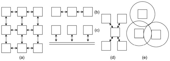
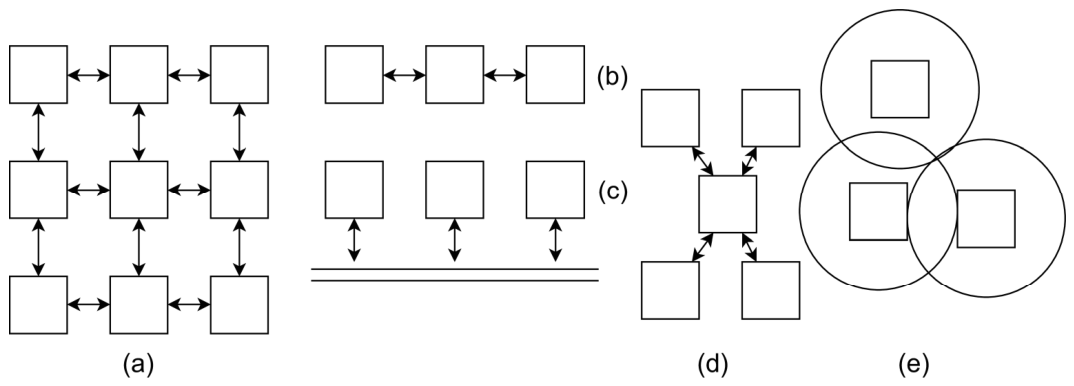
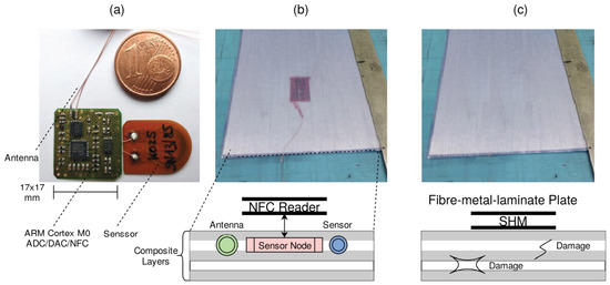
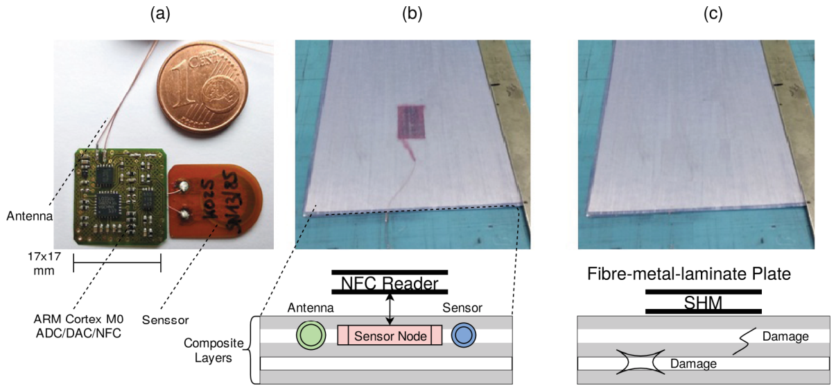
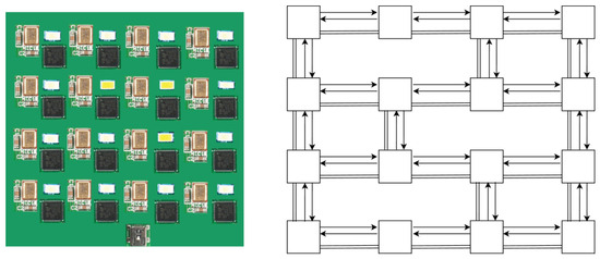
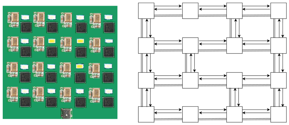
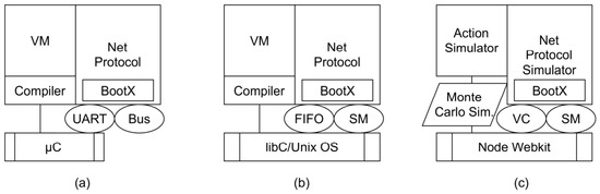
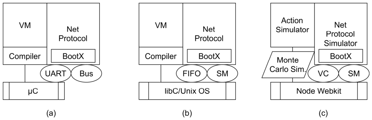
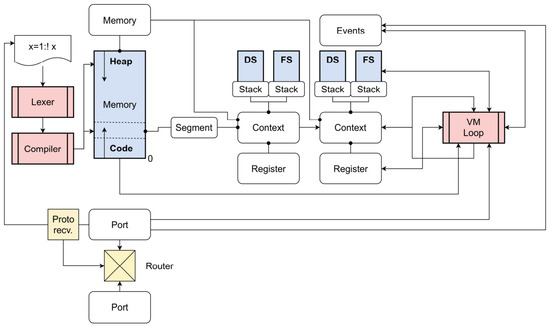
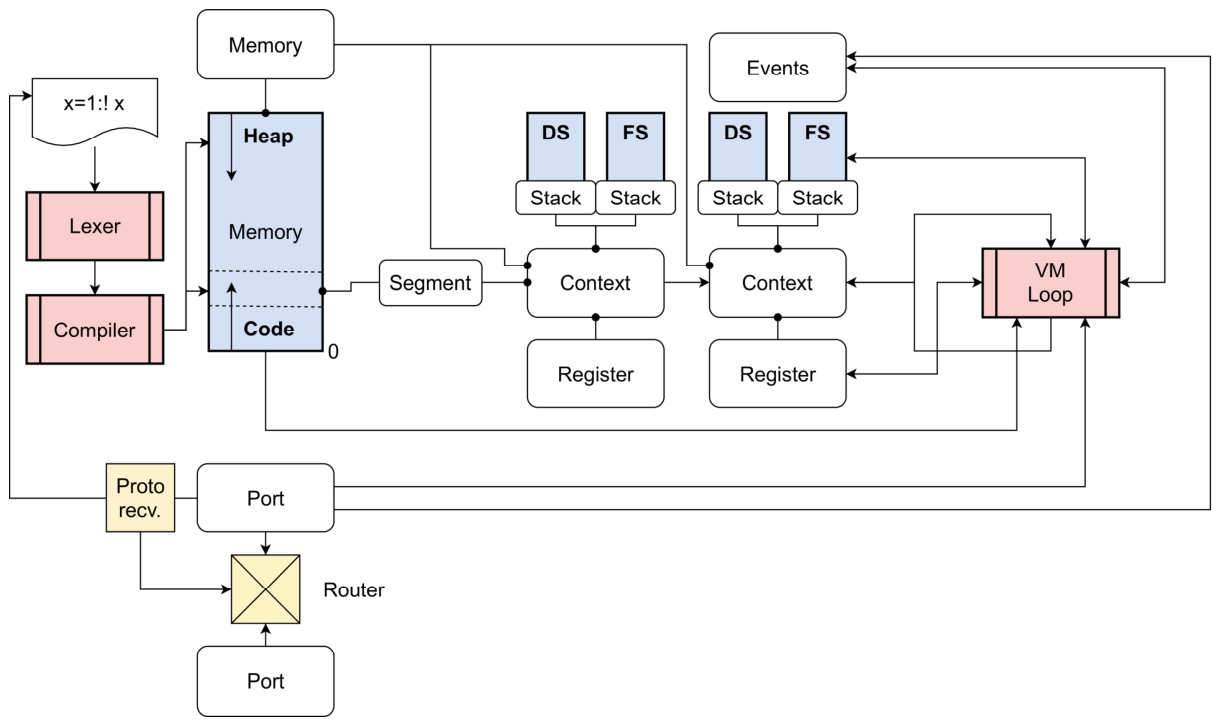
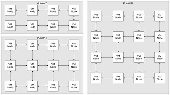
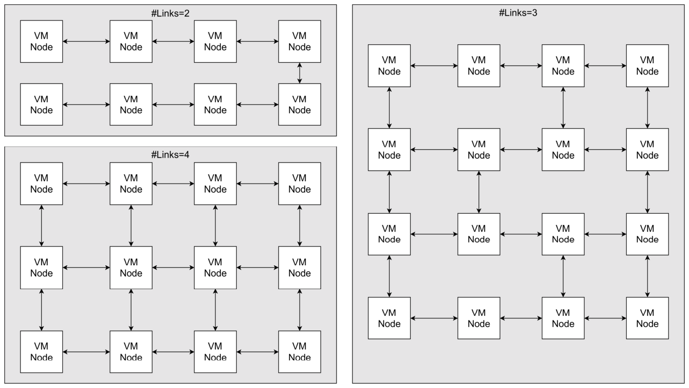
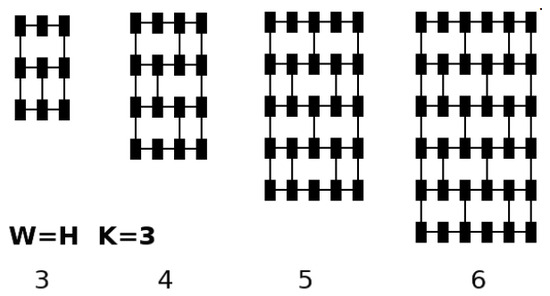
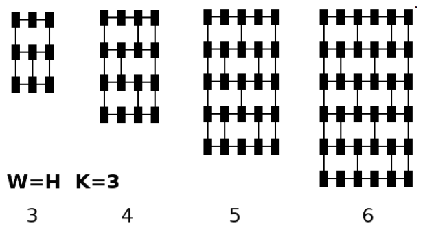
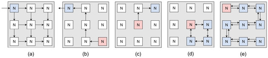
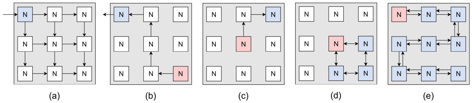
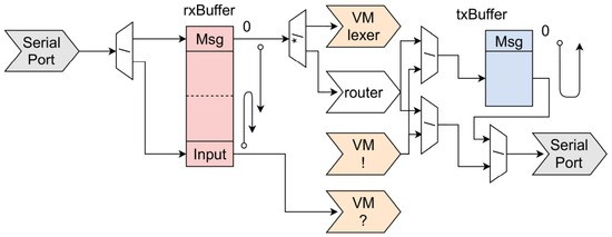
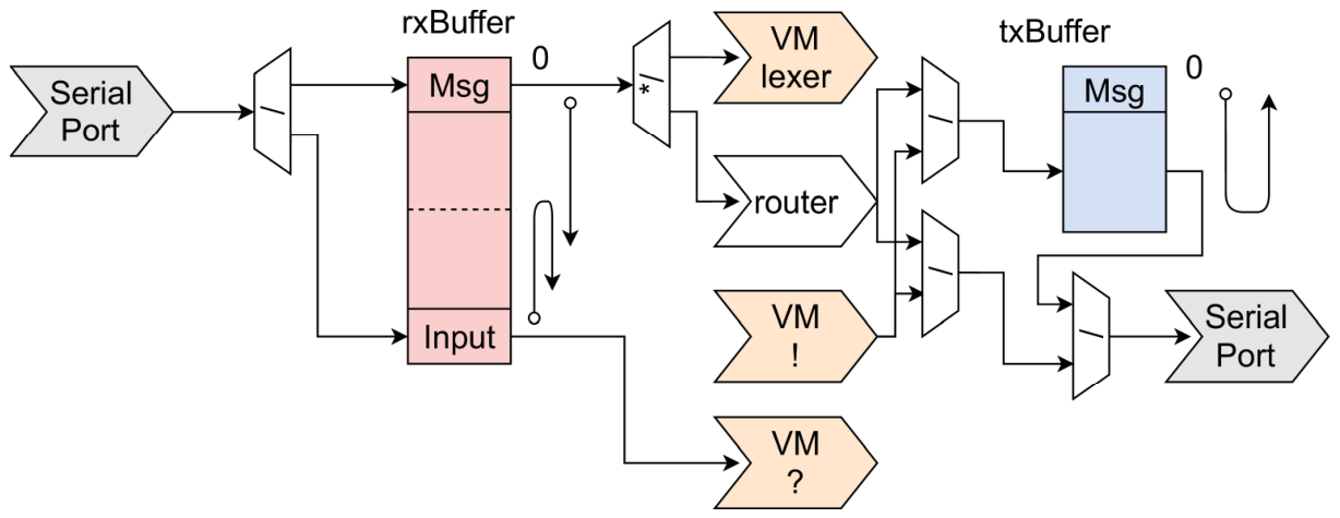
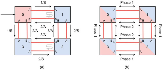
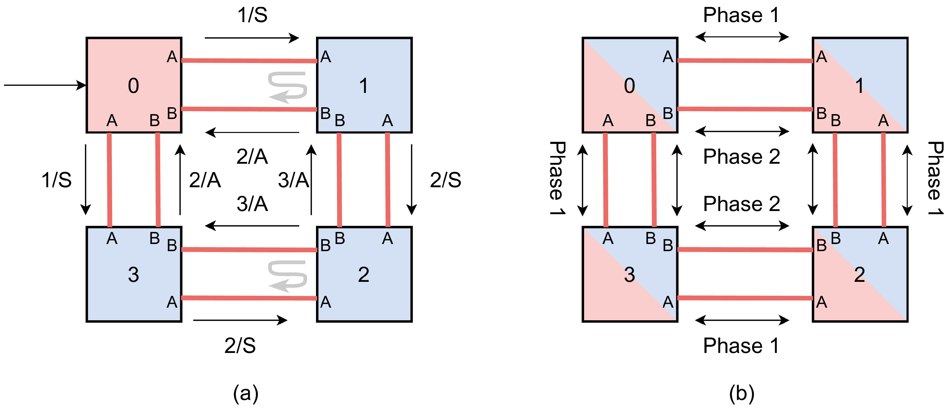
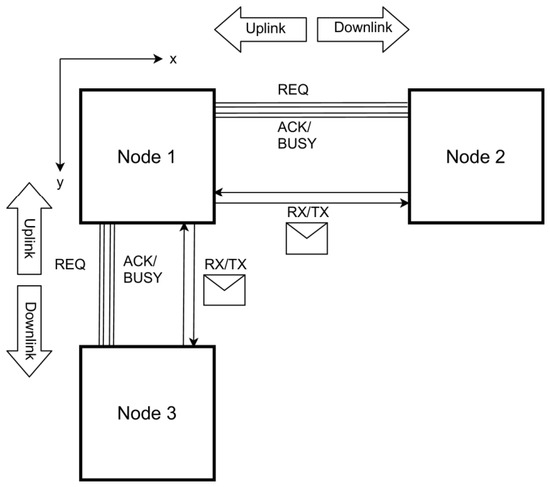
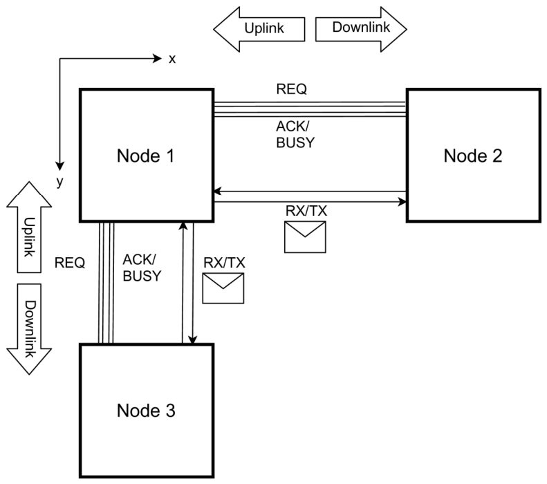
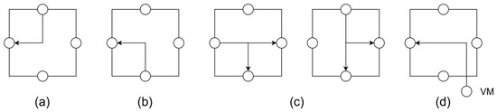
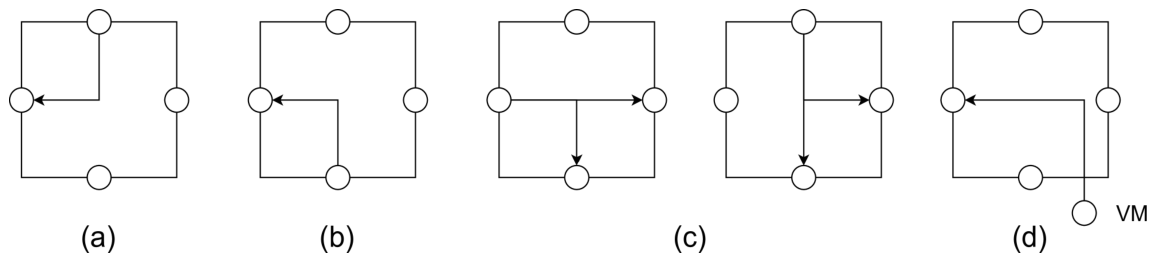
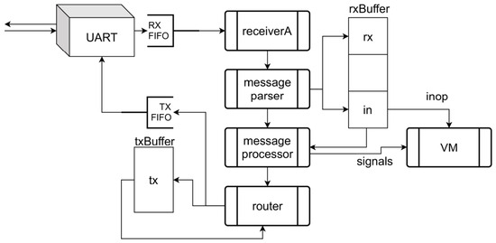
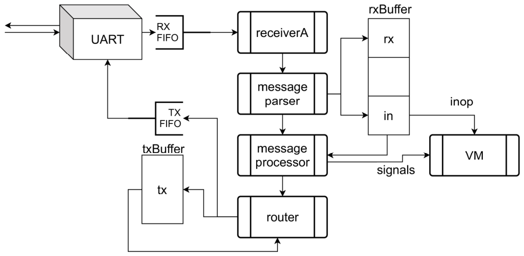
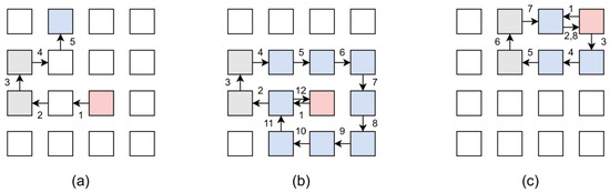
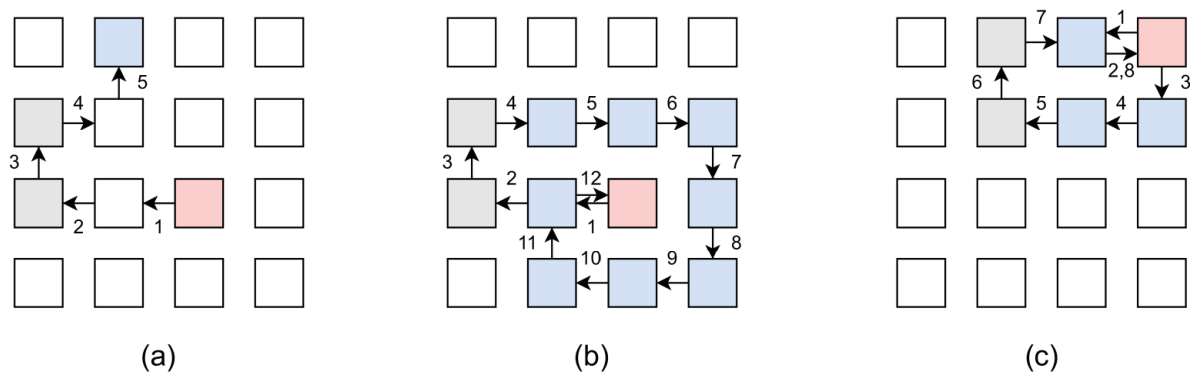
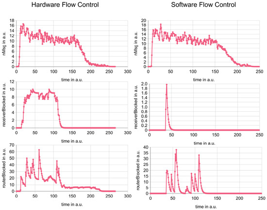
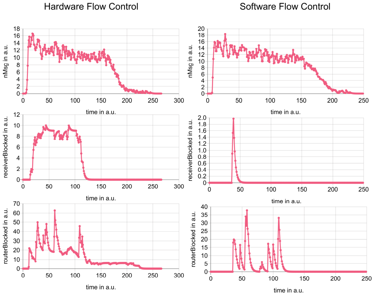
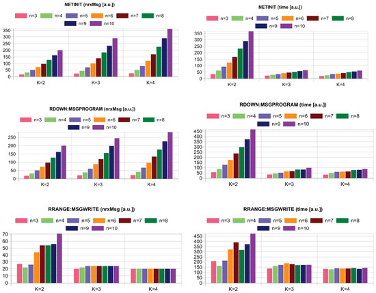
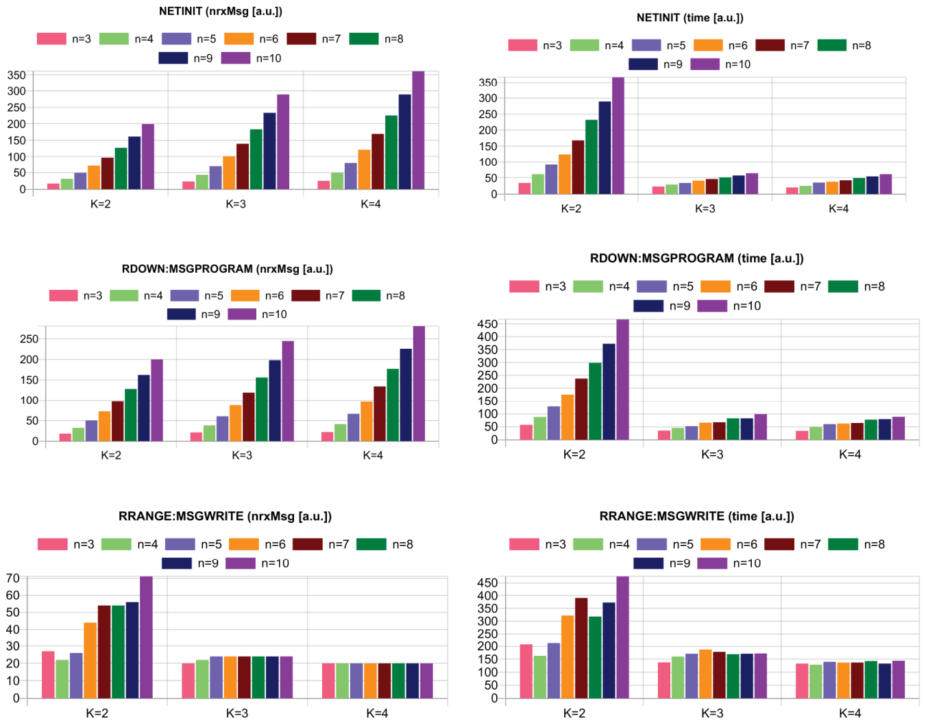
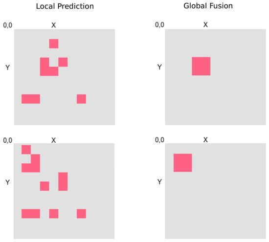
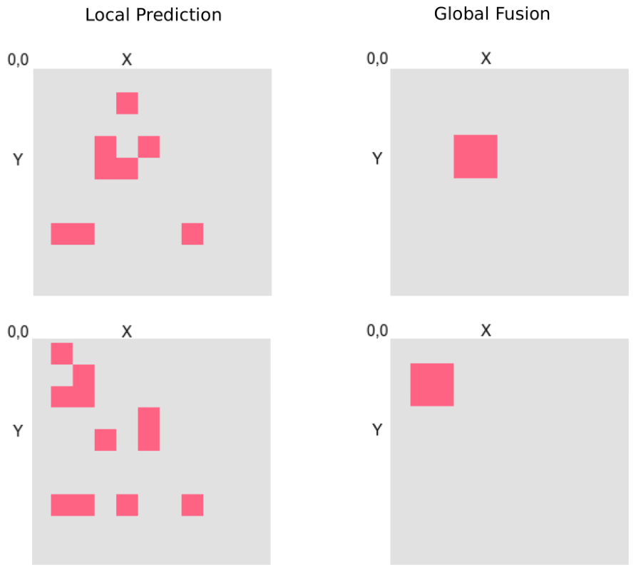

Disclaimer/Publisher’s Note: The statements, opinions and data contained in all publications are solely those of the individual author(s) and contributor(s) and not of MDPI and/or the editor(s). MDPI and/or the editor(s) disclaim responsibility for any injury to people or property resulting from any ideas, methods, instructions or products referred to in the content. |
© 2026 by the author. Licensee MDPI, Basel, Switzerland. This article is an open access article distributed under the terms and conditions of the Creative Commons Attribution (CC BY) license.