Continuous-Variable Quantum Fourier Layer: Applications to Filtering and PDE Solving

Abstract

Fourier representations play a central role in operator learning for partial differential equations and are increasingly being explored in quantum machine learning architectures. The classical fast Fourier transform (FFT), particularly in its Cooley–Tukey decomposition, exhibits a structure that naturally matches continuous-variable quantum circuits. This correspondence establishes a direct structural isomorphism between the Cooley–Tukey butterfly network and Gaussian photonic gates, enabling the FFT to be realized as a native optical computation in continuous-variable quantum computing. Building on this observation, we introduce a continuous-variable Quantum Fourier Layer (CV–QFL) based on a bipartite Gaussian encoding and a Cooley–Tukey quantum Fourier transform, enabling exact two-dimensional spectral processing within a Gaussian photonic circuit. We test the CV–QFL on two representative tasks: spectral low-pass filtering and Fourier-domain integration of the heat equation. In both cases, the results match the classical reference to machine precision. More broadly, this work lays the foundation for continuous-variable approaches to quantum scientific computing and for the development of native spectral architectures in quantum machine learning.

1. Introduction

Fourier transforms are fundamental tools in signal processing, imaging, and scientific computing, enabling the representation of signals and data in the spectral domain and supporting efficient operations, such as filtering and spectral methods for the numerical solution of partial differential equations. For discrete signals, the introduction of the fast Fourier transform (FFT), most prominently through the Cooley–Tukey (CT) algorithm [1], reduced the computational cost of the discrete Fourier transform (DFT) from $\mathcal{O}\left(N^2\right)$ to $\mathcal{O}(NlogN)$ for signals of size N, by recursively decomposing the transform into smaller operations. FFT methods have then become a cornerstone of modern signal processing and scientific computing [2,3,4].

Beyond digital implementations, Fourier transforms can also be obtained directly in optical systems, where interference and propagation naturally perform spectral transformations [5,6]. Moreover, the butterfly structure of the CT decomposition maps naturally onto optical operations such as beam splitting and phase shifting, motivating photonic implementations of the FFT in integrated optical circuits [7,8,9]. While these approaches have mainly been explored for classical optical signal processing, their connection with continuous-variable (CV) quantum computing remains comparatively less developed. Establishing such a connection is especially relevant given the central role played by the quantum Fourier transform (QFT) in quantum algorithms and, more recently, in spectral-based quantum machine learning (QML) models. In this work, we bridge this gap by identifying a structural correspondence between the CT algorithm and its realization in CV photonic quantum circuits, where the elementary operations of the butterfly network map naturally onto Gaussian transformations implemented through beam splitters and phase shifts. This perspective provides the basis for more advanced photonic architectures for spectral processing, with potential applications in QML. In particular, the proposed Continuous-Variable Quantum Fourier layer (CV-QFL) is designed to process classical data defined on two-dimensional domains, making it naturally suited to problems involving structured fields and mappings between functions, as in neural operator frameworks [10,11]. However, this framework also provides a structural foundation for extensions to intrinsically quantum settings, particularly when non-Gaussian resources are incorporated beyond the current Gaussian architecture, as further discussed in Section 4.

• Quantum machine learning and the problem of encoding. A central challenge in QML is how to encode classical data into quantum states. To construct a CV–QFL, one must first determine an encoding strategy that is compatible with the target computational task. Whether the goal is signal filtering, the spectral solution of partial differential equations, or operator learning, the chosen encoding determines the class of Fourier transformations that can be carried out within the circuit and, consequently, the spectral information accessible to the computation [12,13].

In standard qubit-based frameworks, several encoding strategies have been proposed, including basis encoding, amplitude encoding, time-evolution encoding, and Hamiltonian encoding [14,15,16]. These approaches typically map classical data onto a single computational register, naturally leading to one-dimensional QFT implementations [17,18,19]. Such constructions admit efficient decompositions in terms of Hadamard and controlled-phase gates, but remain intrinsically tied to a single-register spectral structure. This limitation becomes particularly relevant when addressing more complex tasks involving two- or three-dimensional fields, such as operator learning for partial differential equations.

Unary encoding has recently emerged as an alternative paradigm [20,21,22,23,24], where the restriction to a fixed-excitation subspace enables the exact realization of orthogonal transformations and enhanced amplitude control. This makes it especially suitable for operator-learning architectures [10,24,25]. Within this setting, Fourier operators [11] have been implemented in one-dimensional quantum architectures [26] and extended to multidimensional domains through tensorized multi-register constructions [27,28], often leveraging CT factorizations decomposed into phase shifters and reconfigurable beam splitter (RBS) gates that preserve excitation number [1]. While naturally suited to linear-optical platforms, these constructions generally require nontrivial compilation overhead on standard qubit hardware [29].

These observations motivate the investigation of QFT implementations formulated directly in terms of optical primitives within the CV setting. In CV quantum computing, information is encoded in bosonic modes with continuous spectra rather than in discrete two-level systems, leading to an infinite-dimensional Hilbert space with enhanced representational capacity and a natural compatibility with structured spectral transformations [30,31,32,33]. Several CV encoding strategies have been proposed for QML, ranging from feature-map embeddings to Gaussian-state encodings [32,34,35]. However, in most existing approaches, classical data are embedded either as single vectors or as local pointwise features [36,37]. While such strategies are suitable for regression or classification, they do not represent the full discretized field as a globally structured object at the quantum-state level. This becomes a serious limitation in operator learning and scientific machine learning, where the data naturally arise as multidimensional fields defined over spatial grids. In such settings, the lack of a structured global encoding prevents the direct application of multidimensional spectral transformations within the quantum circuit. Even when global encodings are considered, they remain predominantly one-dimensional or restricted to discrete-variable constructions [35,38], thereby constraining the class of multidimensional Fourier operators that can be obtained.

• Cooley–Tukey Fourier transforms in CV quantum computing. To address the problem of implementing two-dimensional Fourier transforms in a CV quantum framework, we introduce a bipartite Gaussian encoding scheme in which the input matrix $D\in {\mathbb{R}}^{m\times n}$ is embedded directly into the cross-correlation blocks of a multimode covariance matrix, with m and n denoting the dimensions of the upper and lower registers, respectively. By exploiting inter-register entanglement as a computational resource, the input field is represented at the state level as a structured two-dimensional object, preserving its separable spatial organization already at the encoding stage. This induces a tensor-product organization of the bipartite register and naturally enables a genuinely two-dimensional QFT within a Gaussian CV architecture.

Within this setting, the elementary operations of the CT decomposition map directly onto Gaussian photonic transformations implemented through beam splitters and phase shifts acting on the two registers. By exploiting this separable structure, the Fourier transform can be performed independently along each register, thereby realizing a two-dimensional QFT of the input state within a CV photonic circuit. The resulting transform requires a number of elementary optical gate operations, beam splitters and phase shifts, scaling as $\mathcal{O}(mlogm+nlogn)$ for an $m\times n$ domain, compared with the $\mathcal{O}(mnlog(mn\left)\right)$ operation count of the classical two-dimensional CT algorithm. This reduction represents a hardware resource advantage: fewer physical optical components are needed to implement the circuit on actual photonic hardware. It does not, however, imply a runtime speedup over digital FFT implementations in software; the numerical experiments presented here are conducted using Strawberry Fields [39], a classical simulator of Gaussian circuits whose computational cost is not governed by the quantum gate count. To the best of our knowledge, this is the first CV–QFL that explicitly integrates CV quantum circuits with the CT Fourier-transform framework.

More broadly, the proposed construction opens two complementary directions. First, for signals that are natively optical, such as coherent fields produced by interferometers, wavefront sensors, or free-space optical systems, a continuous-variable photonic architecture offers a natural processing substrate. In a conventional pipeline, such signals must be digitized via analog-to-digital conversion, processed numerically, and potentially re-encoded into an optical carrier, all of which introduce latency and overhead. A CV Fourier layer operating directly on optical modes can in principle bypass this cycle entirely, performing spectral operations, filtering, differentiation, or operator application, without the signal ever leaving the optical domain. The specific encoding introduced in this work targets the classical simulation setting, but the architectural principle extends naturally to natively optical scenarios where the encoding would be adapted to the physical signal representation; this advantage holds entirely within the Gaussian regime. Second, the bipartite register structure and the Cooley–Tukey decomposition developed here provide the spectral-layer foundation for extensions incorporating non-Gaussian resources, such as cubic-phase gates or photon-number-resolving measurements, where classical simulation becomes exponentially demanding and a genuine computational advantage over digital methods may be achieved.

To summarize, the main contributions of this work are as follows:

• Bipartite Gaussian matrix encoding. We introduce a CV encoding scheme that embeds a matrix $D\in {\mathbb{R}}^{m\times n}$ exactly into the cross-covariance block of a bipartite Gaussian state, yielding a structured and physically implementable representation of two-dimensional data in CV systems.
• CV–QFL. We design a CV–QFL acting independently on two registers, enabling an exact two-dimensional quantum Fourier transform of the encoded matrix within a Gaussian photonic architecture.
• Spectral signal filtering and PDE solving. We validate the proposed Fourier layer on two representative tasks: denoising of a two-dimensional signal corrupted by Gaussian noise, and spectral solution of the two-dimensional heat equation directly in the Fourier domain.

2. Materials and Methods

The methodological foundations of the proposed framework are discussed in the following. We first introduce a brief theoretical overview of the basic concepts of CV quantum circuits, Gaussian states and covariance matrices. Then, we describe the bipartite encoding procedure used to map two-dimensional classical data onto the covariance matrix of a multimode Gaussian state. Next, building on this representation, we show the implementation of the two-dimensional Fourier transform through a CV–QFL, which constitutes the core spectral layer of the proposed approach.

2.1. Continuous-Variable: Theoretical Background

We begin by reviewing the basic concepts of CV circuits, including Gaussian states and covariance matrices, before turning to unitary state evolution. For a general introduction to the basic concepts of quantum mechanics, we refer the reader to [40], while for continuous-variable quantum systems we refer to [30].

2.1.1. Gaussian States and the Covariance Matrix

CV quantum systems are described in terms of bosonic modes, each corresponding to a quantum harmonic oscillator. For an n-mode system, we introduce the vector of canonical quadrature operators

$$\widehat{\mathit{r}}={({\widehat{x}}_1,\dots ,{\widehat{x}}_n,{\widehat{p}}_1,\dots ,{\widehat{p}}_n)}^{\top },$$

where the notation $\widehat{·}$ indicates a quantum operator acting on the Hilbert space. In the CV setting, it is convenient to adopt the Heisenberg representation, in which the operators evolve under the circuit while the quantum state is kept fixed. The quadratures are defined as

$${\widehat{x}}_k={\displaystyle \frac{{\widehat{a}}_k+{\widehat{a}}_k^{†}}{\sqrt{2}}},{\widehat{p}}_k={\displaystyle \frac{{\widehat{a}}_k-{\widehat{a}}_k^{†}}{i\sqrt{2}}},$$

(1)

in terms of the annihilation and creation operators ${\widehat{a}}_k$ and ${\widehat{a}}_k^{†}$ of the k-th bosonic mode, which respectively remove and add one excitation. Here, the symbol ^† denotes the Hermitian conjugate of an operator. These operators satisfy the canonical commutation relations

$$[{\widehat{x}}_k,{\widehat{p}}_j]=i{\delta }_{kj},$$

where $[\widehat{A},\widehat{B}]:=\widehat{A}\widehat{B}-\widehat{B}\widehat{A}$ denotes the commutator of two generic operators $\widehat{A}$ and $\widehat{B}$, and ${\delta }_{kj}$ is the Kronecker delta, defined by ${\delta }_{kj}=1$ if $k=j$ and ${\delta }_{kj}=0$ otherwise. Equivalently, the bosonic ladder operators satisfy

$$[{\widehat{a}}_k,{\widehat{a}}_j^{†}]={\delta }_{kj},[{\widehat{a}}_k,{\widehat{a}}_j]=[{\widehat{a}}_k^{†},{\widehat{a}}_j^{†}]=0.$$

Just as in classical physics, the state of the system can be described in terms of its behavior in phase space [16]. The essentials of this behavior are captured by the Wigner function, which was originally proposed by Wigner in [41]. There is a special class of states that is important for optical quantum information processing with continuous variables: the so-called Gaussian states, whose Wigner function is Gaussian in phase space and are fully characterized by their first and second statistical moments, namely, the displacement vector $\mathit{\mu }=⟨\widehat{\mathit{r}}⟩$ and the covariance matrix:

$${\sigma }_{ij}=\frac{1}{2}⟨\{{\widehat{r}}_i-{\mu }_i,{\widehat{r}}_j-{\mu }_j\}⟩,$$

where $\{·,·\}$ denotes the anticommutator. Throughout the paper, vectors are denoted in boldface, whereas matrices are generally denoted by uppercase letters. The covariance matrix is treated as a special case and written in boldface as $\mathit{\sigma }$, in order to distinguish it from the singular-value matrix $\Sigma$ introduced in Section 2.2. Individual vector components and matrix entries are written in standard notation and are identified by lower indices. The covariance matrix is a real symmetric $2n\times 2n$ matrix and must satisfy the Robertson–Schrödinger uncertainty principle [42]:

$$\mathit{\sigma }+\frac{i}{2}\Omega \ge 0,\Omega ={\displaystyle \underset{k=1}{\overset{n}{⨁}}}\left(\begin{array}{cc}0& 1\\ -1& 0\end{array}\right),$$

(2)

where $\Omega$ denotes the canonical symplectic form and ⨁ the direct sum, i.e., the block-diagonal composition of matrices. In particular, $\Omega$ is obtained by repeating the $2\times 2$ block $\left(\begin{array}{cc}0& 1\\ -1& 0\end{array}\right)$ along the diagonal.

Examples of Gaussian states are the vacuum, coherent states, and squeezed coherent states. For more information, see [16,31,43].

2.1.2. Gaussian Unitary Evolution

Gaussian unitary operations correspond to affine symplectic transformations in phase space that preserve the canonical commutation relations and map Gaussian states into Gaussian states. By the universality theorem for linear-optical networks [44,45], any unitary matrix $U\in \mathrm{U}\left(m\right)$ can be exactly decomposed into a sequence of beam splitters and phase shifters acting on m bosonic modes. A passive interferometer implementing $U\in \mathrm{U}\left(m\right)$ acts linearly on the annihilation operators as:

$${\widehat{a}}_k⟼{\displaystyle \sum _{j=1}^m}{U}_{kj}{\widehat{a}}_j.$$

(3)

Since the annihilation operators are the fundamental degrees of freedom of the electromagnetic field, all passive optical transformations act directly on $\widehat{a}$ and ${\widehat{a}}^{†}$. The transformation of quadratures is a derived consequence and, by using the definitions in Equation (1), one can show that:

$$\widehat{\mathit{r}}⟼S_U\widehat{\mathit{r}}\mathrm{with}{S}_U=\left(\begin{array}{cc}\mathrm{Re}\left(U\right)& -\mathrm{Im}\left(U\right)\\ \mathrm{Im}\left(U\right)& \mathrm{Re}\left(U\right)\end{array}\right)\in \mathrm{Sp}(2m,\mathbb{R}),$$

(4)

and:

$$\mathit{\sigma }⟼S_U\mathit{\sigma }{S}_U^{\top }.$$

(5)

2.2. Bipartite Entanglement-Based Encoding

This section develops the encoding scheme used to embed a classical data matrix $D\in {\mathbb{R}}^{m\times n}$ exactly into the covariance matrix of a multimode Gaussian state. We proceed in two steps. We first introduce the theoretical ingredients: the bipartite register architecture, the block structure of the covariance matrix, and the two-mode squeezing operator that generates inter-register correlations. We then describe the actual encoding procedure, which is based on the singular value decomposition (SVD) of D: the singular values determine the squeezing parameters applied to independent pairs of modes, while the orthogonal factors U and V are realized as passive interferometers acting on the two registers. The combined effect is that the classical matrix appears exactly in the x-quadrature cross-covariance block ${\mathit{\sigma }}_{x_{r_1}{x}_{r_2}}$ of the resulting Gaussian state.

We consider a bipartite CV architecture composed of two registers, $r_1$ and $r_2$, containing m and n bosonic modes, respectively, for a total of $m+n$ modes. Throughout this section, superscripts $r_1$ and $r_2$ are used to indicate the register to which a given quadrature or mode operator belongs. For such a system, the global quadrature operator can be written as

$$\widehat{\mathit{r}}={({\widehat{x}}_1^{r_1},\dots ,{\widehat{x}}_m^{r_1},{\widehat{x}}_1^{r_2},\dots ,{\widehat{x}}_n^{r_2},{\widehat{p}}_1^{r_1},\dots ,{\widehat{p}}_m^{r_1},{\widehat{p}}_1^{r_2},\dots ,{\widehat{p}}_n^{r_2})}^{\mathsf{T}}.$$

(6)

Accordingly, the covariance matrix of the bipartite system is a real symmetric matrix

$$\mathit{\sigma }\in {\mathbb{R}}^{2(m+n)\times 2(m+n)},$$

whose dimension reflects the fact that each of the $m+n$ bosonic modes contributes two quadratures, namely, one x-quadrature and one p-quadrature. Consistently with the ordering in Equation (6), $\mathit{\sigma }$ can be written in block form as

$$\mathit{\sigma }=\left(\begin{array}{cccc}{\mathit{\sigma }}_{x_{r_1}{x}_{r_1}}& {\mathit{\sigma }}_{x_{r_1}{x}_{r_2}}& {\mathit{\sigma }}_{x_{r_1}{p}_{r_1}}& {\mathit{\sigma }}_{x_{r_1}{p}_{r_2}}\\ {\mathit{\sigma }}_{x_{r_2}{x}_{r_1}}& {\mathit{\sigma }}_{x_{r_2}{x}_{r_2}}& {\mathit{\sigma }}_{x_{r_2}{p}_{r_1}}& {\mathit{\sigma }}_{x_{r_2}{p}_{r_2}}\\ {\mathit{\sigma }}_{p_{r_1}{x}_{r_1}}& {\mathit{\sigma }}_{p_{r_1}{x}_{r_2}}& {\mathit{\sigma }}_{p_{r_1}{p}_{r_1}}& {\mathit{\sigma }}_{p_{r_1}{p}_{r_2}}\\ {\mathit{\sigma }}_{p_{r_2}{x}_{r_1}}& {\mathit{\sigma }}_{p_{r_2}{x}_{r_2}}& {\mathit{\sigma }}_{p_{r_2}{p}_{r_1}}& {\mathit{\sigma }}_{p_{r_2}{p}_{r_2}}\end{array}\right),$$

(7)

where each block collects the second moments between the corresponding subsets of quadratures. In particular, ${\mathit{\sigma }}_{x_{r_1}{x}_{r_2}}\in {\mathbb{R}}^{m\times n}$ denotes the block containing the correlations between the x-quadratures of registers $r_1$ and $r_2$, while ${\mathit{\sigma }}_{x_{r_1}{x}_{r_1}}\in {\mathbb{R}}^{m\times m}$ and ${\mathit{\sigma }}_{x_{r_2}{x}_{r_2}}\in {\mathbb{R}}^{n\times n}$ describe the intra-register x-quadrature second moments. Analogous interpretations hold for the remaining blocks involving the p-quadratures.

• To encode correlations between the two registers, we employ the two-mode squeezing (TMS) operator

$${\widehat{S}}_2(r,\varphi )=exp\left[r\left(e^{i\varphi }{\widehat{a}}_i^{r_1}{\widehat{a}}_j^{r_2}-e^{-i\varphi }{\left({\widehat{a}}_i^{r_1}\right)}^{†}{\left({\widehat{a}}_j^{r_2}\right)}^{†}\right)\right],$$

(8)

acting on mode i of register $r_1$ and mode j of register $r_2$. Here, $r\in \mathbb{R}$ denotes the squeezing parameter and $\varphi$ the phase. For $\varphi =0$, the action of the TMS gate on the quadrature operators of the two modes is given by

$$\left(\begin{array}{c}{\widehat{x}}_i^{r_1}\\ {\widehat{x}}_j^{r_2}\\ {\widehat{p}}_i^{r_1}\\ {\widehat{p}}_j^{r_2}\end{array}\right)⟼S_{\mathrm{TMS}}\left(r\right)\left(\begin{array}{c}{\widehat{x}}_i^{r_1}\\ {\widehat{x}}_j^{r_2}\\ {\widehat{p}}_i^{r_1}\\ {\widehat{p}}_j^{r_2}\end{array}\right),\mathrm{with}{S}_{\mathrm{TMS}}\left(r\right)=\left(\begin{array}{cccc}coshr& sinhr& 0& 0\\ sinhr& coshr& 0& 0\\ 0& 0& coshr& -sinhr\\ 0& 0& -sinhr& coshr\end{array}\right).$$

(9)

Starting from the vacuum state and adopting the convention $\hslash =2$, where ℏ is the reduced Planck constant, one has

$$⟨{\left({\widehat{x}}_i^{r_1}\right)}^2⟩=⟨{\left({\widehat{x}}_j^{r_2}\right)}^2⟩=1,⟨{\widehat{x}}_i^{r_1}{\widehat{x}}_j^{r_2}⟩=0.$$

(10)

For completeness, the meaning of the expectation-value notation $⟨·⟩$, the definition of the vacuum state, and the derivation of the relations above are briefly reviewed in Appendix A. From Equation (9), it follows that, after the TMS transformation,

$$⟨{\widehat{x}}_i^{\prime r_1}{\widehat{x}}_j^{\prime r_2}⟩=sinh\left(2r\right),$$

where the prime denotes the transformed quadrature operators. This shows that the gate generates nontrivial correlations between the two registers.

We now describe the encoding procedure for a classical data matrix $D\in {\mathbb{R}}^{m\times n}$ to be embedded into the bipartite CV architecture. In this naive entry-wise construction, we denote by $r_{ij}$ the squeezing parameter associated with the matrix entry $D_{ij}$. One would then assign independent squeezing parameters according to

$$r_{ij}=\frac{1}{2}arcsinh\left(\lambda D_{ij}\right),$$

(11)

so that

$$⟨{\widehat{x}}_i^{r_1}{\widehat{x}}_j^{r_2}⟩=\lambda D_{ij}.$$

Here, $\lambda >0$ is a global scaling factor introduced to control the squeezing amplitudes and keep the required two-mode squeezing operations within physically reasonable energy bounds. However, such an entry-wise construction is not implementable in practice: two-mode squeezing gates acting on shared modes do not commute, and successive applications alter both local variances and previously established inter-register correlations. As a result, it is not possible to independently encode all entries $D_{ij}$ in this manner, since later operations inevitably distort the covariance structure generated by earlier ones.

To overcome this limitation, the encoding is performed in a decoupled basis obtained through the Singular Value Decomposition (SVD) of the input matrix:

$$D=U\Sigma V^{\top },$$

(12)

where $U\in {\mathbb{R}}^{m\times m}$ and $V\in {\mathbb{R}}^{n\times n}$ are orthogonal matrices whose columns are the left and right singular vectors of D, respectively, while $\Sigma \in {\mathbb{R}}^{m\times n}$ is the rectangular diagonal matrix whose nonzero diagonal entries are the singular values ${\sigma }_1,\dots ,{\sigma }_{\mathcal{\ell }}$, with $\mathcal{\ell }=rank\left(D\right)$. In this basis, each singular value ${\sigma }_k$ corresponds to an independent pair of modes, one in register $r_1$ and one in register $r_2$, allowing the assignment

$$r_k=\frac{1}{2}arcsinh\left(\lambda {\sigma }_k\right),k=1,\dots ,\mathcal{\ell },$$

(13)

where $\mathcal{\ell }=rank\left(D\right)$. Here, $r_k$ denotes the squeezing parameter associated with the k-th pair of corresponding modes in the SVD basis, namely, the modes whose x-quadratures are ${\widehat{x}}_k^{r_1}$ and ${\widehat{x}}_k^{r_2}$, and which encode the singular value ${\sigma }_k$. In this way, one can embed the diagonal matrix $\Sigma$ directly into the inter-register cross-covariance block of the Gaussian state without inter-register interference. The resulting covariance matrix then takes the block form

$${\mathit{\sigma }}_{\mathrm{TMS}}= \left(\begin{array}{cccc}\hfill C_{r_1}& \begin{array}{|c|}\hline \Sigma \\ \hline\end{array}& 0\hfill & 0\\ \hfill {\Sigma }^{\top }& C_{r_2}& 0\hfill & 0\\ \hfill 0& 0& C_{r_1}\hfill & \begin{array}{|c|}\hline -\Sigma \\ \hline\end{array}\\ \hfill 0& 0& -{\Sigma }^{\top }\hfill & C_{r_2}\end{array}\right),$$

(14)

where the subscripts $r_1$ and $r_2$ identify the blocks associated with the quadratures of the first and second register, respectively. The matrices

$$C_{r_1}\in {\mathbb{R}}^{m\times m},C_{r_2}\in {\mathbb{R}}^{n\times n},$$

describe the local second moments, namely, the single-mode variances within each register, as opposed to the off-diagonal blocks $\Sigma$ and ${\Sigma }^{\top }$, which encode inter-register correlations.Their diagonal entries follow directly from the transformation in Equation (9): for each independent mode pair in the SVD basis, the variances are mapped from the vacuum value 1 to $cosh\left(2r_i\right)$, while the corresponding inter-register correlations become $sinh\left(2r_i\right)$. Hence,

$$C_{r_1}=diag\left(cosh\left(2r_1\right),\dots ,cosh\left(2r_{\mathcal{\ell }}\right),1,\dots ,1\right),$$

and analogously for $C_{r_2}$, where the trailing ones correspond to modes that are not involved in the encoding and therefore remain in the vacuum state. Moreover, $\Sigma \in {\mathbb{R}}^{m\times n}$ is the rectangular diagonal matrix of singular values, with ${\Sigma }_{kk}=sinh\left(2r_k\right)$ for $k=1,\dots ,\mathcal{\ell }$ and zero otherwise. We notice that the off-diagonal block ${\sigma }_{x_{r_1}{x}_{r_2}}$ contains the inter-register $xx$ correlations and coincides, in the rotated SVD basis, with the encoded matrix $\Sigma$.

As granted by the universality theorem [44], both factors U and V of Equation (12) are physically realizable as passive interferometers on the respective registers. By the application of this theorem, it will be possible to reconstruct the original input matrix D.

When U acts on $r_1$ and V acts simultaneously on $r_2$, one can show by following Section 2.1 about Gaussian unitary evolution, that the full symplectic transformation on the joint quadrature vector $\widehat{\mathit{r}}$ of Equation (6) is:

$$S_{\mathrm{tot}}=\left(\begin{array}{cccc}U& 0& 0& 0\\ 0& V& 0& 0\\ 0& 0& U& 0\\ 0& 0& 0& V\end{array}\right),$$

(15)

and that the full covariance matrix transforms as $\mathit{\sigma }\mapsto S_{\mathrm{tot}}\mathit{\sigma }{S}_{\mathrm{tot}}^{\top }$. Extracting the cross-block ${\mathit{\sigma }}_{x_{r_1}{x}_{r_2}}$ from this expression, one obtains:

$${\mathit{\sigma }}_{x_{r_1}{x}_{r_2}}^{\prime }=U{\mathit{\sigma }}_{x_{r_1}{x}_{r_2}}{V}^T=U\Sigma V^{\top }=D.$$

(16)

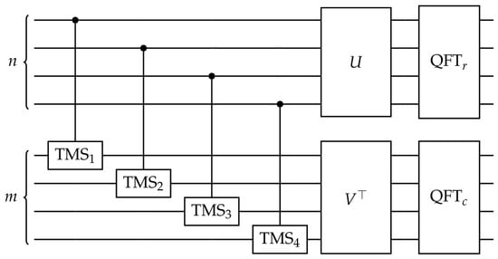
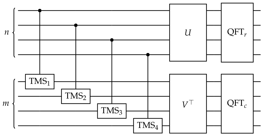
The data matrix D is therefore encoded exactly in the x-quadrature cross-block of the bipartite covariance matrix, with U acting from the left via register $r_1$ and V from the right via register $r_2$; see Figure 1 for the complete CV quantum circuit representation. The cross-block ${\mathit{\sigma }}_{p_{r_1}{p}_{r_2}}=-D$ acquires the opposite sign, while all x-p cross-correlations vanish identically.

Figure 1. CV–QFL circuit for an $m\times n$ input matrix on $m+n$ optical modes. Encoding: TMS gates inject the singular values of M; interferometers U and $V^{\top }$ reconstruct the input matrix via SVD. Fourier Layer: the CT QFT is applied independently to both registers, yielding the 2D optical Fourier transform.

For additional details on the theoretical aspects of the encoding procedure such as complexity and bipartite entanglement, and on its Strawberry Fields implementation, see Appendix B.

2.3. Cooley–Tukey as Continuous-Variable Quantum Circuit

The core idea of our work, namely, the structural isomorphism between the CT algorithm and the set of optical operations available in CV quantum circuits, is presented in this section.

We begin by reviewing the implementation of the CT algorithm to implement the FFT in the one-dimensional setting, before extending the construction to higher-dimensional domains. We then show how its computational structure maps naturally onto CV circuit operations, which forms the central idea underlying this work. To have more information about the classical DFT before approaching the CT algorithm, see Appendix B.3.

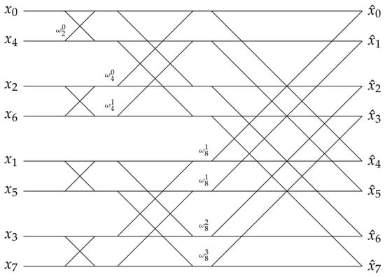
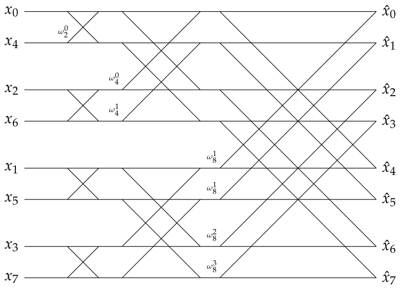
To Fourier transform a one-dimensional vector $x\in {\mathbb{R}}^N$, the procedure begins by permuting its indices according to a bit-reversal scheme. Throughout this work, we adopt the direct-transform sign convention and define the twiddle factors as

$${\omega }_n^k=e^{-i{\displaystyle \frac{2\pi k}{n}}},$$

where i is the imaginary unit, n denotes the size of the local transform at a given stage of the Cooley–Tukey algorithm, and k labels the corresponding twiddle factor. The core computational step, with $N=8$ as an example, is the butterfly-shaped cross operation, see Figure 2.

Figure 2. Butterfly diagram of the CT algorithm for the FFT of the bit-reversed input $x\in {\mathbb{R}}^8$. Each cross is a radix-2 butterfly with twiddle factor ${\omega }_n^k=e^{-i2\pi k/n}$.

In this diagram, each cross

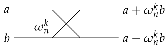
• is applied iteratively to pairs of elements and maps $(a,b)$ as follows:

$$\left(\begin{array}{cc}1& {\omega }_n^k\\ 1& -{\omega }_n^k\end{array}\right)\left(\begin{array}{c}a\\ b\end{array}\right)=\left(\begin{array}{c}a+{\omega }_n^{k}b\\ a-{\omega }_n^{k}b\end{array}\right),{\omega }_n^k=e^{-i{\displaystyle \frac{2\pi k}{n}}},$$

(17)

where $n=2,4,8$ is the number of inputs at each stage and $k\in \{0,1,\dots ,\frac{n}{2}-1\}$.

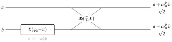
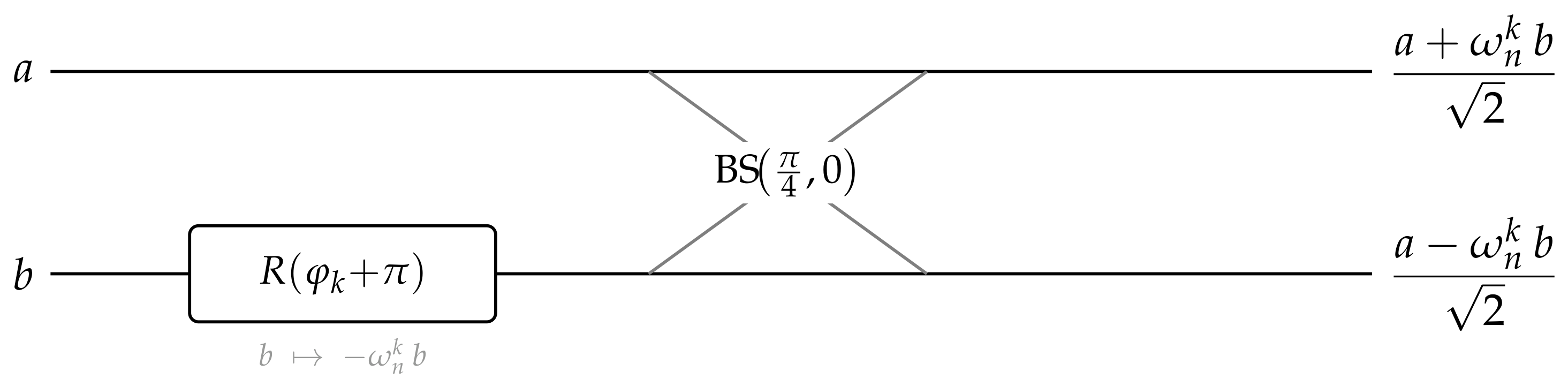
In the CV circuit, each butterfly cross is replaced by a sequence of two optical gates acting on a pair of modes $(q_i,q_j)$, as shown in Figure 3.

Figure 3. CV implementation of a single CT butterfly. The phase gate $R({\phi }_k+\pi )$ maps $b\mapsto -{\omega }_n^{k}b$; the beam splitter $\mathrm{BS}(\pi /4,0)$ then produces $(a\pm {\omega }_n^{k}b)/\sqrt{2}$, identical to the classical output (17) up to the $1/\sqrt{2}$ ortho-normalization factor.

The Rgate maps mode $q_j$ as $b\mapsto e^{i({\phi }_k+\pi )}b=-{\omega }_n^{k}b$, where ${\phi }_k=-2\pi k/n$, so that $e^{i{\phi }_k}={\omega }_n^k$. The BSgate, whose symplectic action is $a^{\prime }=(a-b)/\sqrt{2}$, $b^{\prime }=(a+b)/\sqrt{2}$, then gives:

$${\displaystyle \frac{1}{\sqrt{2}}}\left(\begin{array}{cc}1& {\omega }_n^k\\ 1& -{\omega }_n^k\end{array}\right)\left(\begin{array}{c}a\\ b\end{array}\right)={\displaystyle \frac{1}{\sqrt{2}}}\left(\begin{array}{c}a+{\omega }_n^{k}b\\ a-{\omega }_n^{k}b\end{array}\right).$$

In this way, we reconstruct the transformation found in the classical butterfly (17), realized entirely through operations native to CV photonic circuits.

A key observation concerns the $1/\sqrt{2}$ factor that appears in the CV output but is absent in the classical butterfly (17). This factor is not an additional correction introduced by hand; it is a direct physical consequence of beam splitter unitarity. A 50:50 beam splitter is a unitary gate that conserves the total optical energy of the two modes it acts on, which forces the $1/\sqrt{2}$ prefactor on each output. Crucially, this factor accumulates over the ${log}_{2}N$ butterfly stages of the full CT circuit, producing the global $1/\sqrt{N}$ normalization of the unitary (ortho-normalized) DFT. In classical digital implementations, this normalization factor must be inserted explicitly as a post-processing step; in the optical circuit, it emerges automatically from the physics of energy conservation at each beam splitter. This is one of the deepest structural correspondences between the CT algorithm and its CV photonic realization: the physical constraint of unitarity is precisely what implements the correct normalization of the quantum Fourier transform.

We are now ready to extend the one-dimensional CT transformation to the two-dimensional setting. As shown in Equation (A22) of the Appendix B.3, the 2D discrete Fourier transform admits a separable structure, and can therefore be implemented through independent one-dimensional transforms applied along each dimension. The classical CT radix-2 algorithm [1] exploits this separability by first applying a 1D FFT of length n to each of the m rows of D, at a cost of $\mathcal{O}(nlogn)$ per row, and subsequently applying a 1D FFT of length m to each of the n columns of the intermediate result, at a cost of $\mathcal{O}(mlogm)$ per column. The total arithmetic cost is therefore

$$\mathrm{gate}\mathrm{count}:m·\mathcal{O}(nlogn)+n·\mathcal{O}(mlogm)=\mathcal{O}(mnlog(mn\left)\right).$$

(18)

2.4. Continuous-Variable Quantum Fourier Layer

We now show how the CV–QFL can be physically implemented in CV quantum computing, by applying independent single-register Fourier transforms to a bipartite Gaussian state encoding the matrix D in its cross-correlation block. To this end, we now apply Fourier matrices $F_m$ to register $r_1$ and $F_n$ to register $r_2$ simultaneously. Then, in the same way of Equations (15) and (A22) of Appendix B.3, the global symplectic matrix takes the explicit block form:

$$S_{\mathrm{tot}}=\left(\begin{array}{cccc}\mathrm{Re}\left(F_m\right)& 0& -\mathrm{Im}\left(F_m\right)& 0\\ 0& \mathrm{Re}\left(F_n\right)& 0& -\mathrm{Im}\left(F_n\right)\\ \mathrm{Im}\left(F_m\right)& 0& \mathrm{Re}\left(F_m\right)& 0\\ 0& \mathrm{Im}\left(F_n\right)& 0& \mathrm{Re}\left(F_n\right)\end{array}\right),$$

(19)

so that the full quadrature transformation is compactly expressed as:

$${\widehat{\mathit{r}}}^{\prime }=S_{\mathrm{tot}}\widehat{\mathit{r}},{\mathit{\sigma }}^{\prime }=S_{\mathrm{tot}}\mathit{\sigma }{S}_{\mathrm{tot}}^{\top }.$$

(20)

Substituting Equations (19) and (20) into ${\left({\mathit{\sigma }}_{x_{r_1}{x}_{r_2}}^{\prime }\right)}_{ij}=⟨{\widehat{x}}_i^{\prime r_1}{\widehat{x}}_j^{\prime r_2}⟩$ and using the four inter-register second moments of the encoded state:

$$⟨{\widehat{x}}_k^{r_1}{\widehat{x}}_l^{r_2}⟩=D_{kl},⟨{\widehat{p}}_k^{r_1}{\widehat{p}}_l^{r_2}⟩=-D_{kl},⟨{\widehat{x}}_k^{r_1}{\widehat{p}}_l^{r_2}⟩=⟨{\widehat{p}}_k^{r_1}{\widehat{x}}_l^{r_2}⟩=0,$$

(21)

one obtains:

$$\begin{array}{cc}\hfill {\left({\mathit{\sigma }}_{x_{r_1}{x}_{r_2}}^{\prime }\right)}_{ij}& =\sum _{k,l}\mathrm{Re}{\left(F_m\right)}_{ik}\mathrm{Re}{\left(F_n\right)}_{jl}\underset{D_{kl}}{\underbrace{⟨{\widehat{x}}_k^{r_1}{\widehat{x}}_l^{r_2}⟩}}-\sum _{k,l}\mathrm{Re}{\left(F_m\right)}_{ik}\mathrm{Im}{\left(F_n\right)}_{jl}\underset{0}{\underbrace{⟨{\widehat{x}}_k^{r_1}{\widehat{p}}_l^{r_2}⟩}}\hfill \\ \hfill & -\sum _{k,l}\mathrm{Im}{\left(F_m\right)}_{ik}\mathrm{Re}{\left(F_n\right)}_{jl}\underset{0}{\underbrace{⟨{\widehat{p}}_k^{r_1}{\widehat{x}}_l^{r_2}⟩}}+\sum _{k,l}\mathrm{Im}{\left(F_m\right)}_{ik}\mathrm{Im}{\left(F_n\right)}_{jl}\underset{-D_{kl}}{\underbrace{⟨{\widehat{p}}_k^{r_1}{\widehat{p}}_l^{r_2}⟩}},\hfill \end{array}$$

(22)

which simplifies to:

$${\mathit{\sigma }}_{x_{r_1}{x}_{r_2}}^{\prime }=\mathrm{Re}\left(F_m\right)D\mathrm{Re}{\left(F_n\right)}^{\top }-\mathrm{Im}\left(F_m\right)D\mathrm{Im}{\left(F_n\right)}^{\top }=\mathrm{Re}\left(F_{m}D{F}_n^{\top }\right).$$

(23)

Note that, unlike the one-dimensional case, the $pp$ block $⟨{\widehat{p}}^{r_1}{\widehat{p}}^{r_2}⟩=-D$ now contributes a non-trivial term because both registers are transformed. Then, substituting Equations (19) and (20) into ${\left({\mathit{\sigma }}_{x_{r_1}{p}_{r_2}}^{\prime }\right)}_{ij}=⟨{\widehat{x}}_i^{\prime r_1}{\widehat{p}}_j^{\prime r_2}⟩$, one similarly has:

$${\left({\mathit{\sigma }}_{x_{r_1}{p}_{r_2}}^{\prime }\right)}_{ij}=\mathrm{Re}\left(F_m\right)D\mathrm{Im}{\left(F_n\right)}^{\top }+\mathrm{Im}\left(F_m\right)D\mathrm{Re}{\left(F_n\right)}^{\top }=\mathrm{Im}\left(F_{m}D{F}_n^{\top }\right).$$

(24)

The two blocks (23) and (24) combine into a single complex quantity:

$$\begin{array}{cc}\hfill {\mathit{\sigma }}_{x_{r_1}{x}_{r_2}}^{\prime }+i{\mathit{\sigma }}_{x_{r_1}{p}_{r_2}}^{\prime }& =\mathrm{Re}\left(F_{m}D{F}_n^{\top }\right)+i\mathrm{Im}\left(F_{m}D{F}_n^{\top }\right)=F_{m}D{F}_n^{\top },\hfill \end{array}$$

(25)

so that:

$$\begin{array}{|c|}\hline \widehat{D}=F_{m}D{F}_n^{\top }={\mathit{\sigma }}_{x_{r_1}{x}_{r_2}}^{\prime }+i{\mathit{\sigma }}_{x_{r_1}{p}_{r_2}}^{\prime }.\\ \hline\end{array}$$

(26)

This is precisely the two-dimensional DFT of D (see Equation (A22)). The result can be read directly from the covariance matrix:

$${\mathit{\sigma }}^{\prime }= \left(\begin{array}{cccc}\hfill {\sigma }_{x_{r_1}{x}_{r_1}}^{\prime }& \begin{array}{|c|}\hline \mathrm{Re}\left(\widehat{D}\right)\\ \hline\end{array}& {\sigma }_{x_{r_1}{p}_{r_1}}^{\prime }\hfill & \begin{array}{|c|}\hline \mathrm{Im}\left(\widehat{D}\right)\\ \hline\end{array}\\ \hfill \begin{array}{|c|}\hline \mathrm{Re}{\left(\widehat{D}\right)}^{\top }\\ \hline\end{array}& {\sigma }_{x_{r_2}{x}_{r_2}}^{\prime }& \begin{array}{|c|}\hline \mathrm{Im}{\left(\widehat{D}\right)}^{\top }\\ \hline\end{array}\hfill & {\sigma }_{x_{r_2}{p}_{r_2}}^{\prime }\\ \hfill {\sigma }_{p_{r_1}{x}_{r_1}}^{\prime }& \begin{array}{|c|}\hline \mathrm{Im}\left(\widehat{D}\right)\\ \hline\end{array}& {\sigma }_{p_{r_1}{p}_{r_1}}^{\prime }\hfill & \begin{array}{|c|}\hline -\mathrm{Re}\left(\widehat{D}\right)\\ \hline\end{array}\\ \hfill \begin{array}{|c|}\hline \mathrm{Im}{\left(\widehat{D}\right)}^{\top }\\ \hline\end{array}& {\sigma }_{p_{r_2}{x}_{r_2}}^{\prime }& \begin{array}{|c|}\hline -\mathrm{Re}{\left(\widehat{D}\right)}^{\top }\\ \hline\end{array}\hfill & {\sigma }_{p_{r_2}{p}_{r_2}}^{\prime }\end{array}\right)$$

where the boxed entries are entirely determined by $\widehat{D}=F_{m}D{F}_n^{\top }$, and the unboxed diagonal blocks describe local single-register variances. The two-dimensional DFT of D is therefore obtained directly from the second moments of the bipartite Gaussian state, without any additional processing; it suffices to read the cross-block ${\mathit{\sigma }}_{x_{r_1}{x}_{r_2}}^{\prime }$ and ${\mathit{\sigma }}_{x_{r_1}{p}_{r_2}}^{\prime }$ of the covariance matrix ${\mathit{\sigma }}^{\prime }$ after the CT circuits have been applied to both registers, and combine them as:

$$\widehat{D}={\mathit{\sigma }}_{x_{r_1}{x}_{r_2}}^{\prime }+i{\mathit{\sigma }}_{x_{r_1}{p}_{r_2}}^{\prime },$$

(27)

where the real part encodes the cosine components of the transform and the imaginary part the sine components. Both blocks are entries of the physical covariance matrix and are directly accessible via homodyne measurements on the two registers.

A complete graphical representation of the CV–QFL circuit is provided in Figure 1. The figure highlights the three main stages of the architecture: singular-value encoding via two-mode squeezing gates, the U and V interferometers used to reconstruct the input matrix D, and the CT QFT decomposition applied independently to the two registers.

The two-dimensional CT QFT application results in a circuit of depth $\mathcal{O}(logm)$ on $r_1$ and a circuit of depth $\mathcal{O}(logn)$ on $r_2$. Since the two registers are disjoint, the two circuits run in parallel, giving

$$\mathrm{gate}\mathrm{count}:\mathcal{O}(mlogm+nlogn),\mathrm{depth}:\mathcal{O}(log(mn\left)\right).$$

(28)

Complexity Analysis

A direct comparison between Equations (18) and (28) shows that the bipartite CV implementation achieves a QFT gate count of $\mathcal{O}(mlogm+nlogn)$, as opposed to the $\mathcal{O}(mnlog(mn\left)\right)$ operation count of the classical two-dimensional FFT, thereby reducing the circuit resources required to implement the Fourier transform. To correctly interpret the gate-count comparison in Equations (18)–(28), it is important to distinguish between three separate notions of computational cost involved in the full pipeline, summarized in Table 1. The first is the classical preprocessing cost of the SVD factorization $D=U\Sigma V^{\top }$, which scales as $\mathcal{O}(mnmin(m,n\left)\right)$ and must be computed on a classical computer before the circuit can be loaded; this cost dominates the pipeline for large inputs and constitutes its primary computational bottleneck. The second is the encoding circuit gate count, $\mathcal{O}(m^2+n^2)$, arising from the passive interferometers implementing the SVD factors U and V on the two registers (see Appendix B for details). The third is the QFT circuit gate count, $\mathcal{O}(mlogm+nlogn)$, which counts the optical operations (beam splitters and phase shifts) required to perform the Fourier transform; this is the quantity compared with the $\mathcal{O}(mnlog(mn\left)\right)$ operation count of the classical two-dimensional FFT, and the gate-count advantage cited above refers exclusively to this stage.

Table 1. Computational costs of the three stages of the CV–QFL pipeline and comparison with the classical two-dimensional FFT. The gate-count advantage discussed in the text refers exclusively to the CV–QFT row and should not be conflated with the encoding or preprocessing costs.

Phase	Type	Operation Count	Circuit Depth
SVD factorization $D=U\Sigma V^{\top }$	Classical preprocessing	$\mathcal{O}(mnmin(m,n\left)\right)$	—
Encoding (TMS + interferometers)	Optical circuit	$\mathcal{O}(m^2+n^2)$	$\mathcal{O}(max(m,n\left)\right)$
CV–QFT (CT butterfly network)	Optical circuit	$\mathcal{O}(mlogm+nlogn)$	$\mathcal{O}(log(mn\left)\right)$
Classical 2D FFT (reference)	Classical algorithm	$\mathcal{O}(mnlog(mn\left)\right)$	—

The gate-count advantage in the CV–QFT row is of a theoretical and architectural nature: the numerical experiments were carried out using Strawberry Fields [39], a classical simulator of Gaussian circuits whose runtime is governed by covariance-matrix operations rather than by the quantum gate count. No experimental confirmation of the speedup is therefore provided here; its demonstration on actual photonic hardware is left to future work.

3. Results

To illustrate the practical utility of the CV–QFL pipeline, we present two concrete applications: low-pass spectral filtering and numerical solution of a diffusive partial differential equation. In both cases, the computation is carried out entirely inside the photonic circuit using Strawberry Fields.

3.1. Spectral Low-Pass Filtering

We consider a $64\times 64$ test image composed of three known low-frequency components,

$$s(x,y)=cos\left(\frac{2\pi ·3x}{64}\right)cos\left(\frac{2\pi ·3y}{64}\right)+\frac{1}{2}cos\left(\frac{2\pi ·7x}{64}\right)+\frac{1}{2}cos\left(\frac{2\pi ·5y}{64}\right),$$

(29)

corrupted by additive white Gaussian noise with unitary standard deviation, yielding an input SNR (signal-to-noise ratio) of $-3.0\mathrm{dB}$.

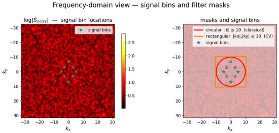
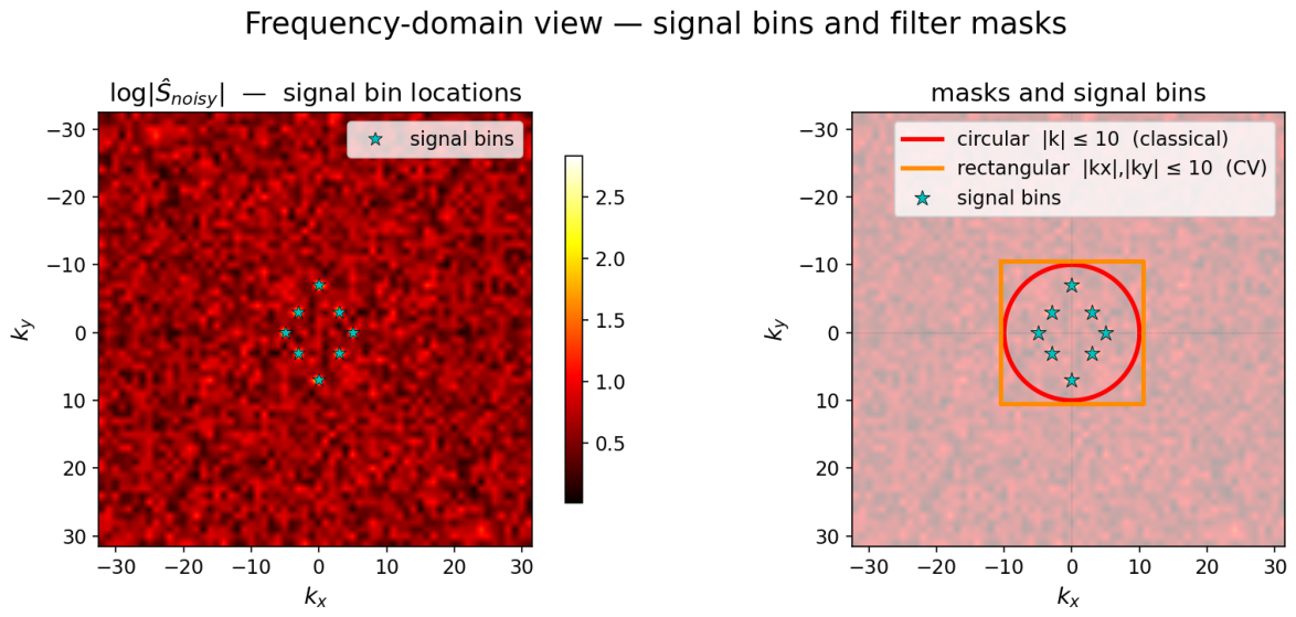
Because each cosine term generates discrete Fourier peaks (equivalently, delta-like contributions on specific frequency bins), the spectrum of s is exactly sparse. In centered frequency notation, its nonzero components are located at:

$$\left\{\right(\pm 3,\pm 3),(\pm 7,0),(0,\pm 5\left)\right\},$$

(30)

as shown in Figure 4. Thus, the signal energy is concentrated on only eight Fourier bins associated with the prescribed low-frequency components, while the added noise is broadband and distributed across the full spectrum. By preserving the few low-frequency bins containing the signal and suppressing the remaining noise-dominated modes, the inverse Fourier transform reconstructs the original image with high fidelity and improved SNR ratio.

Figure 4. (Left) spectral representation of the noisy input, highlighting both the background noise and the frequency bins associated with the signal. (Right) comparison of the spectral masks used in the filtering experiment, namely, a circular mask with $\left|\mathbf{k}\right|\le 10$ and a separable rectangular mask with $|k_x|\le 10$ and $|k_y|\le 10$. In both cases, the signal frequency components are fully contained within the mask.

To implement low-pass filtering in the CV–QFL, we use the LossChannel operation available in Strawberry Fields. Physically, LossChannel$\left(T\right)$ models optical attenuation by mixing the signal mode with a vacuum mode through a beam splitter of transmissivity $T\in [0,1]$. In the Gaussian formalism, its action on the covariance matrix $\mathit{\sigma }$ and mean vector $\mu$ is:

$$\mathit{\sigma }⟶T\mathit{\sigma }+(1-T)\mathbf{I},\mu ⟶\sqrt{T}\mu .$$

(31)

and shows that, for $T=1$, the transformation is the identity, while for $T=0$, the mode is replaced by vacuum and all correlations with the rest of the system are removed.

A key property of LossChannel is that it is phase-insensitive: both quadratures of a mode are attenuated by the same factor $\sqrt{T}$. As a result, when LossChannel is applied independently to row and column modes, each complex Fourier coefficient

$$z[i,j]={\sigma }_{xx}[i,m+j]+i{\sigma }_{xp}[i,m+j]$$

(32)

is simply rescaled as:

$$z[i,j]⟶\sqrt{T_i{T}_j}z[i,j].$$

(33)

This is essential, since it suppresses selected Fourier amplitudes without altering their phase.

To realize a low-pass filter, we choose binary transmissivities $T_i,T_j\in \{0,1\}$ so that only modes within the desired frequency range are preserved, while higher-frequency modes are removed. This implements a separable rectangular spectral mask in Fourier space. After the inverse QFT, the filtered signal is reconstructed directly from the output covariance matrix, without any intermediate digital manipulation of the spectrum.

We next compare the proposed CV–QFL filtering pipeline with a standard classical Fourier baseline on the noisy $64\times 64$ signal. In the classical case, the corrupted image is transformed to Fourier space through a two-dimensional FFT, filtered by a circular low-pass mask with cutoff $\left|\mathbf{k}\right|\le 10$, and mapped back to physical space by the inverse FFT. The CV–QFL follows the same spectral-processing structure, but all Fourier operations are implemented at the level of the optical circuit: the encoded signal is first transformed by the forward QFT, the unwanted modes are attenuated through mode-wise LossChannel operations, and the filtered field is reconstructed by applying the inverse QFT, obtained as the adjoint circuit.

The only structural difference between the two pipelines lies in the geometry of the spectral mask. The classical reference uses a circular cutoff, whereas the present CV implementation realizes a separable rectangular cutoff, $|k_x|\le 10$, $|k_y|\le 10$, as a consequence of applying independent loss channels along the two registers. Importantly, both masks contain all the Fourier bins associated with the clean signal, as illustrated in Figure 4. The comparison is summarized quantitatively in Table 2 and visually in Figure 5.

Table 2. Spectral filtering comparison on a $64\times 64$ grid.

	Classical	CV-QFL
Mask shape	circular	rectangular (separable)
Bins retained	317/4096 (7.7%)	441/4096 (10.8%)
SNR in (dB)	$-3.0$	$-3.0$
SNR out (dB)	$7.7$	$6.4$
SNR improvement (dB)	$+10.7$	$+9.4$

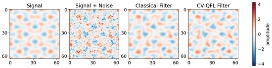
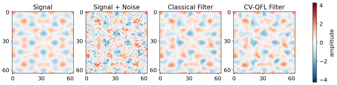
Figure 5. Spectral low-pass filtering on a $64\times 64$ image. (Left) to (right) clean signal; noisy input ($\mathrm{SNR}=-3.0\mathrm{dB}$); classical output (circular mask, $+10.7\mathrm{dB}$); CV–QFL output (rectangular separable mask, $+9.4\mathrm{dB}$).

The noisy input has an SNR of $-3.0\mathrm{dB}$, so that the noise energy is comparable to, and in practice larger than, the energy of the underlying signal. This is reflected in the second panel of Figure 5, where the original sinusoidal structure is almost completely obscured. The corresponding reconstruction error is $\mathrm{RMSE}=0.998$, approximately $141\%$ of the signal standard deviation (${\sigma }_s\simeq 0.71$). After low-pass filtering, both pipelines recover the dominant low-frequency pattern with high visual fidelity. The classical pipeline reduces the RMSE from $0.998$ to $0.292$, while the CV–QFL reduces it to $0.339$. Equivalently, because the mean-squared error satisfies $\mathrm{MSE}={\mathrm{RMSE}}^2$, this corresponds to reducing the MSE by a factor of approximately $11.7$ for the classical pipeline and $8.7$ for the CV–QFL.

The difference between the two results is therefore small: the classical pipeline improves the SNR by $10.7\mathrm{dB}$, whereas the CV–QFL achieves a $9.4\mathrm{dB}$ improvement, leaving a gap of only $1.3\mathrm{dB}$. This residual discrepancy is not due to an error in the quantum Fourier circuit, but to the broader separable mask implemented by the CV pipeline, which retains 441 spectral bins instead of the 317 bins retained by the circular classical mask. Consequently, the CV–QFL preserves slightly more noise-dominated high-frequency content. When the comparison is performed against a classical reference using the same rectangular mask, the maximum pointwise discrepancy is $3.8\times {10}^{-15}$, confirming that the CV–QFL reproduces the target spectral operation at machine precision.

3.2. Two-Dimensional Heat Equation

We consider the dimensionless two-dimensional heat equation

$${\displaystyle \frac{\partial u}{\partial t}}=\alpha {\nabla }^{2}u,$$

(34)

where $u=u(x,y,t)$ denotes the scalar field of interest, t is time, $\alpha =0.05$ is the diffusion coefficient, and ${\nabla }^2$ is the two-dimensional Laplacian operator, given by

$${\nabla }^{2}u={\displaystyle \frac{{\partial }^{2}u}{\partial x^2}}+{\displaystyle \frac{{\partial }^{2}u}{\partial y^2}}.$$

The heat equation is posed on a square periodic domain $(x,y)\in {[0,L]}^2$, with periodic boundary conditions and initial condition given by the superposition of two localized Gaussian peaks. In the numerical experiments, the domain is discretized on a $32\times 32$ spatial grid.

A convenient way to solve this equation is in the Fourier domain, where the Laplacian acts diagonally and the dynamics decouple mode by mode. As a result, each Fourier coefficient, indexed by the Fourier wavevector $\mathbf{k}=(k_x,k_y)$, evolves independently over a time step $\Delta t$ according to the exponential damping law

$$\widehat{u}(\mathbf{k},t+\Delta t)=e^{-{\alpha \left|\mathbf{k}\right|}^2\Delta t}\widehat{u}(\mathbf{k},t),$$

(35)

where ${\left|\mathbf{k}\right|}^2=k_x^2+k_y^2$. This defines the exact spectral propagator:

$$G(\mathbf{k},\Delta t)=e^{-{\alpha \left|\mathbf{k}\right|}^2\Delta t},$$

(36)

which attenuates high-frequency modes more strongly than low-frequency ones. The corresponding solution strategy therefore follows the same structure as the filtering task: the field is transformed to the Fourier domain, evolved through the mode-wise propagator, and then reconstructed by the inverse Fourier transform.

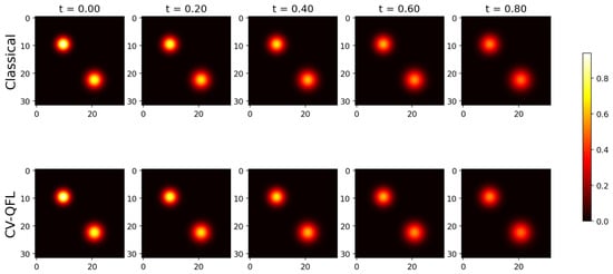
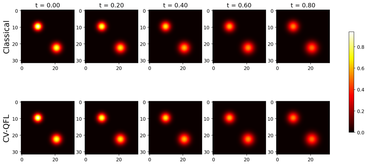
In this example, because the two-Gaussian profile contains substantial mid-to-high spatial frequency content, it provides a convenient test for Fourier-domain diffusion. The system is evolved for four time steps of size $\Delta t=0.2$ up to a final time $t=0.8$, during which the peaks progressively broaden and decrease in amplitude, as expected from diffusive heat dynamics, see Figure 6.

Figure 6. Heat equation integration on a $32\times 32$ grid ($\alpha =0.05$, $\Delta t=0.2$, four steps). (Top row) classical pseudospectral solver (NumPy). (Bottom row) CV–QFL photonic circuit.

After the forward QFT, applying LossChannel$\left(T_i\right)$ to row mode i and LossChannel$\left(T_j\right)$ to column mode j scales the cross-covariance as shown in Equation (33). Then, choosing $T_i=e^{-2\alpha k_{r,i}^2\Delta t}$ and $T_j=e^{-2\alpha k_{c,j}^2\Delta t}$ gives:

$$\sqrt{T_i{T}_j}=e^{-\alpha (k_{r,i}^2+k_{c,j}^2)\Delta t}=G(\mathbf{k},\Delta t),$$

(37)

i.e., the exact heat-equation propagator, where subscripts r and c stand for rows and column registers. The only difference from the low-pass filter is the transmissivity profile programmed into LossChannel: binary $\{0,1\}$ for filtering, $e^{-2\alpha k^2\Delta t}$ for diffusion.

At every time step, the CV–QFL output agrees with the classical pseudospectral solver to floating-point precision, as reported in Table 3. The two Gaussian blobs spread and merge under diffusion; Figure 6 shows that the classical and CV–QFL snapshots are visually indistinguishable at all time steps, confirming that LossChannel$(T_k=e^{-2\alpha k^2\Delta t})$ implements the exact heat-equation propagator inside the optical circuit.

Table 3. Maximum absolute error between the classical pseudospectral solution and the solution computed with the CV–QFL at different time instants for the heat equation, with the error at the level of floating-point precision over the entire temporal evolution.

Time t	$max|{\mathit{u}}_{\mathbf{CV}}-{\mathit{u}}_{\mathbf{classical}}|$
0.0	$0.0\times {10}^0$
0.2	$4.4\times {10}^{-16}$
0.4	$5.0\times {10}^{-16}$
0.6	$5.6\times {10}^{-16}$
0.8	$6.4\times {10}^{-16}$

Scalability and Noise Considerations

The benchmark experiments are carried out on small grids ($64\times 64$ for filtering and $32\times 32$ for the heat equation) and assume ideal photonic gates; both aspects deserve comment for realistic larger-scale implementations. On the computational side, the CV–QFT circuit depth scales as $\mathcal{O}(log(mn\left)\right)$ and the gate count as $\mathcal{O}(mlogm+nlogn)$ on physical photonic hardware, both favorable with respect to grid size. The primary bottlenecks lie elsewhere: the classical Gaussian simulator used here operates on a $2(m+n)\times 2(m+n)$ covariance matrix whose cost grows more steeply than a direct NumPy FFT, and the SVD preprocessing required by the encoding step carries a classical cost of $\mathcal{O}(mnmin(m,n\left)\right)$ regardless of the backend. The Cooley–Tukey butterfly structure also requires power-of-two dimensions; non-dyadic grids need zero-padding. On the noise side, realistic photonic implementations introduce finite squeezing, phase errors, and optical loss, which would degrade the output accuracy relative to the machine-precision results reported here. The logarithmic circuit depth limits error accumulation favorably: gate imperfections propagate through only $\mathcal{O}(log(mn\left)\right)$ sequential layers on physical hardware. For spectral filtering, noise would manifest primarily as imperfect suppression of out-of-band modes and residual leakage at the mask boundary, leaving in-band signal reconstruction largely unaffected. For the heat equation, small errors in the LossChannel transmissivity profile would produce deviations from the exact exponential damping law, growing with the number of time steps. The machine-precision baseline established here provides a quantitative reference against which such hardware imperfections can be characterized in future experimental implementations.

4. Discussion

The results presented in the previous section show that the proposed CV-QFL reproduces both spectral filtering and Fourier-domain integration of the heat equation with machine-precision agreement with the classical reference. These experiments should therefore be interpreted primarily as proof-of-principle validations of correctness and operational fidelity. At the same time, they help clarify the nature of the present contribution: for the small benchmark problems considered here, the main advantage of the proposed framework is not an immediate computational speedup over classical FFT-based implementations, but rather its architectural significance. Specifically, the method provides a native continuous-variable photonic realization of a two-dimensional Fourier layer, based on a structured bipartite Gaussian encoding and on a Cooley–Tukey decomposition directly mapped to Gaussian optical gates. In this sense, the framework should be viewed as a foundation for more advanced spectral quantum architectures, which may become increasingly relevant for larger-scale problems or for settings naturally compatible with photonic and continuous-variable hardware. Two complementary directions stand out and are discussed in the following.

The first direction concerns signals that are natively optical, such as coherent fields generated by interferometers, wavefront sensors, or free-space optical systems, where the signal already lives in optical modes and no classical-to-quantum encoding step is required. In a conventional pipeline, such a signal would be measured, digitized, processed numerically, and then re-encoded into an optical carrier; each transition introduces overhead and potential degradation. By contrast, the CV-QFL processes the signal directly within the photonic circuit: beam splitters and phase shifts act on the optical modes as the field propagates, producing a filtered or transformed optical output without any intermediate digital representation. This implementation advantage, the complete elimination of the encoding bottleneck, is genuine and holds entirely within the Gaussian regime, independently of any claim about computational complexity. It is especially compelling for spectral tasks such as filtering or spectral differentiation, where both input and output are optical fields sharing the same physical substrate as the processing hardware.

The second direction concerns settings where the input is already a quantum state, not a classical field to be encoded, but a multimode system whose relevant information resides in its quantum correlations. Here too the bipartite CV-QFL can apply spectral transformations directly at the state level, bypassing the encoding step. However, as long as both the input state and the circuit remain within the Gaussian regime, the overall computation stays efficiently simulable on classical hardware through the covariance matrix formalism, and no computational advantage over digital methods is gained. A genuine computational advantage would arise only upon incorporating non-Gaussian resources, such as cubic-phase gates or photon-number-resolving measurements, which render classical simulation exponentially demanding. The bipartite register organization, the Cooley–Tukey decomposition, and the mode-wise filtering structure developed here constitute the spectral-layer foundation on which such a non-Gaussian extension could be built.

A second important perspective is the connection with operator learning. Unlike standard CV encodings, which typically represent data as vectors of local amplitudes or single-mode features, the present construction embeds an entire two-dimensional field into the cross-covariance structure of a bipartite Gaussian state. As a result, the CV-QFL acts on a structured field rather than on isolated scalar inputs. This is particularly relevant for scientific machine learning models such as Fourier Neural Operators [11]. From this viewpoint, the proposed framework may provide a natural continuous-variable photonic foundation for spectral operator learning.

At the same time, achieving a definitive quantum advantage for purely classical problems remains challenging. Even highly efficient quantum neural operators are fundamentally constrained by the classical-to-quantum data encoding bottleneck, which introduces substantial overhead and poses severe hardware requirements for near-term devices. Consequently, outperforming well-established classical architectures on purely classical datasets remains difficult. The natural long-term direction for this framework therefore points toward settings where the input is already a non-Gaussian quantum state and the processing involves non-Gaussian circuit operations; in this regime, classical simulation becomes exponentially demanding, and the quantum circuit provides a native and efficient spectral processing mechanism. The bipartite Gaussian architecture developed here, its register organization, Cooley–Tukey decomposition, and mode-wise filtering, establishes the structural blueprint on which such a non-Gaussian extension could be built.

The present framework also has important limitations. First, the proposed cross-covariance encoding is intrinsically two-dimensional, so extending it to higher-dimensional or spatio-temporal fields will require new register organizations and more general encoding strategies. Second, the current architecture is entirely Gaussian and therefore efficiently simulable on classical hardware, which prevents any claim of computational quantum advantage in its present form. Incorporating non-Gaussian resources may overcome this limitation and lead to more expressive quantum models, although at the price of significantly greater experimental complexity. Finally, the present implementation relies on separable mode-by-mode spectral processing; exploring richer forms of inter-register coupling may enable more general classes of spectral operators in future developments.

5. Conclusions

In this work, we introduced a continuous-variable quantum Fourier layer based on a structural correspondence between the Cooley–Tukey decomposition and continuous-variable quantum circuits, where beam splitters and phase shifts naturally reproduce the elementary operations of the butterfly network. Building on this observation, we developed a bipartite Gaussian encoding that represents a two-dimensional input field within the cross-correlations of a multimode photonic state, thereby enabling an exact two-dimensional quantum Fourier transform within a continuous-variable framework.

The main contribution of this work is therefore architectural. Rather than importing a classical Fourier layer into a quantum setting in an abstract way, the proposed construction shows that spectral processing can be realized directly through operations that are native to photonic continuous-variable hardware. In this sense, the framework provides a genuine spectral primitive for continuous-variable quantum computing and establishes a concrete basis for future quantum machine learning architectures built around Fourier-domain processing.

From the experimental point of view, we validated the proposed layer on two representative tasks. In the first, involving spectral low-pass filtering of a noisy two-dimensional signal, the method reproduced the target spectral action with machine-precision agreement with the classical reference. In the second, involving Fourier-domain integration of the two-dimensional heat equation, the circuit matched the classical pseudospectral solution at machine precision across all time steps. These results show that the proposed layer is not only formally well motivated, but also operationally accurate on nontrivial spectral tasks.

More broadly, this work opens a photonic route to spectral processing in continuous-variable quantum computing, with potential relevance for quantum machine learning, signal processing, and Fourier-based approaches to partial differential equations. Although the present implementation is entirely Gaussian and therefore remains efficiently simulable on classical hardware, it provides a clear starting point for more expressive quantum architectures. Future work will focus on extending the framework to higher-dimensional domains, introducing non-Gaussian resources, and exploring applications to intrinsically quantum-mechanical problems, where continuous-variable quantum models may offer a more natural computational framework.

Appendix B.1. Bipartite Entanglement

While the two-mode squeezed vacuum is naturally described in the quadrature basis, it admits an equivalent representation in the Fock basis which is very useful to understand the role of entanglement in our encoding procedure. This representation makes the bipartite entanglement structure explicit, as the state admits the Schmidt decomposition [43]:

$${\widehat{S}}_2\left(r\right)|00⟩=\sqrt{1-\lambda }{\displaystyle \sum _{n=0}^{\infty }}{\lambda }^{n/2}|n⟩|n⟩,\lambda ={tanh}^{2}r,$$

(A16)

where the Fock states $\left\{|n⟩\right\}$ form the Schmidt basis. In this form, the entanglement can be quantified by the von Neumann entropy of the reduced density operator [46]:

$$E\left(r\right)={cosh}^{2}rlog\left({cosh}^{2}r\right)-{sinh}^{2}rlog\left({sinh}^{2}r\right).$$

(A17)

In our encoding scheme, see Section 2.2, each singular value ${\sigma }_k$ determines a squeezing parameter $r_k$ and therefore a corresponding contribution to the total entanglement between the two registers. The entanglement spectrum of the resulting bipartite Gaussian state is thus directly determined by the singular value spectrum of $\Sigma$, establishing a one-to-one correspondence between spectral magnitude and quantum correlations. We notice that Gaussian operations applied independently on the two registers, such as the passive interferometers implementing U and V, see Section 2.2, correspond to local symplectic transformations and therefore leave the inter-register entanglement invariant [14,31,43]. As a result, the entanglement spectrum is entirely determined by the squeezing parameters $r_k$ associated with the singular values.

Appendix B.2. Circuit Complexity of the Encoding

The encoding circuit acts on $m+n$ bosonic modes, partitioned into two registers $r_1$ (m modes) and $r_2$ (n modes). The construction consists of a layer of two-mode squeezing gates followed by two passive interferometers implementing the unitary factors of the SVD.

First, the $N=min(m,n)$ two-mode squeezing (TMS) gates act on disjoint mode pairs and are therefore mutually independent. They can be applied in a single parallel layer, contributing N Gaussian entangling gates with circuit depth equal to one.

Then, the unitary matrices $U\in \mathrm{U}\left(m\right)$ and $V\in \mathrm{U}\left(n\right)$ are realized through the Clements rectangular decomposition [44], which on a $\mathcal{\ell }$-dimensional mode input, implements an ℓ-mode unitary using exactly ${\displaystyle \frac{\mathcal{\ell }(\mathcal{\ell }-1)}{2}}$ beam-splitter–phase-shifter pairs arranged in ℓ columns of $\lfloor \mathcal{\ell }/2\rfloor$ parallel gates. Since U and V act on disjoint registers, with dimensions m and n respectively, the two interferometers can be executed simultaneously. Their combined cost is therefore:

$${\displaystyle \frac{m(m-1)}{2}}+{\displaystyle \frac{n(n-1)}{2}}=\mathcal{O}(m^2+n^2),\mathrm{with}\mathrm{depth}\mathcal{O}(max(m,n)).$$

The total encoding circuit is accordingly dominated by the interferometric stages, yielding an overall optical gate count of $\mathcal{O}(m^2+n^2)$ and a circuit depth of $\mathcal{O}(max(m,n\left)\right)$ on $m+n$ modes. However, this circuit-level complexity should be distinguished from the cost of the full input-loading pipeline. In particular, the factorization $D=U\Sigma V^{\top }$ must be computed classically in advance, with complexity $\mathcal{O}(mnmin(m,n\left)\right)$, which constitutes a significant preprocessing overhead and a potential computational bottleneck for large inputs. Although this step does not contribute to the optical circuit depth once U, V, and $\Sigma$ are fixed, it remains an essential part of the overall workflow.

This observation also clarifies the scope of the proposed encoding: its main value is not to provide an immediate computational speedup for arbitrary classical data loading, but rather to identify a structured CV optical representation in which Fourier-domain processing can be implemented natively. In scenarios where the input is already available in optical form, or is generated directly by an optical front-end, this classical preprocessing may be reduced or avoided altogether, making the framework more naturally suited to native photonic data rather than generic classically stored matrices.

Appendix B.3. Discrete Fourier Transform

Now, we introduce the classical DFT in both one and two dimensions. We start with the definition of the DFT of a vector $\mathbf{v}\in {\mathbb{C}}^l$:

$${\widehat{v}}_k={\displaystyle \frac{1}{\sqrt{l}}}{\displaystyle \sum _{j=0}^{l-1}}{v}_j{e}^{-2\pi ijk/l},k=0,1,\dots ,l-1.$$

(A18)

Introducing the unitary Fourier matrix $F_l\in {\mathbb{C}}^{l\times l}$ with entries:

$${\left(F_l\right)}_{kj}={\displaystyle \frac{1}{\sqrt{l}}}{e}^{-2\pi ijk/l},$$

(A19)

the one-dimensional DFT can be written compactly as

$$\widehat{\mathbf{v}}=F_l\mathbf{v}\mathrm{with}{F}_l^{†}{F}_l=I_l.$$

(A20)

Given a matrix $M\in {\mathbb{C}}^{m\times n}$, the two-dimensional DFT is defined by applying the transform along both dimensions, so that:

$${\widehat{M}}_{k\mathcal{\ell }}={\displaystyle \frac{1}{\sqrt{mn}}}{\displaystyle \sum _{i=0}^{m-1}}{\displaystyle \sum _{j=0}^{n-1}}{M}_{ij}{e}^{-2\pi i\left({\displaystyle \frac{ik}{m}}+{\displaystyle \frac{j\mathcal{\ell }}{n}}\right)},$$

(A21)

which, by the factorization of the Fourier kernel, admits the compact bilinear form:

$$\widehat{M}=F_{m}M{F}_n^{\top }.$$

(A22)

As described in Section 2.3 and Section 2.4, this separable structure is exploited by acting independently on the two registers, so that the row- and column-wise transforms can be performed in parallel.

Appendix B.4. Code Implementation

The encoding circuit is constructed within a Strawberry Fields Program acting on $m+n$ modes. The three stages, Two-Mode Squeezing, interferometer on $r_1$, and interferometer on $r_2$, are implemented as follows:

prog = sf.Program(m + n) with prog.context as q:    # Stage 1: Two-Mode Squeezing    for i in range(k):      S2gate(r[i], 0) | (q[i], q[m + i]) $$    # Stage 2: Interferometer on register r1    Interferometer(U) | q[:m] $$    # Stage 3: Interferometer on register r2    Interferometer(Vt.T) | q[m:]

The quantum circuit realization is illustrated in Figure 1.

The covariance matrix of the resulting Gaussian state is computed by running the circuit on the Gaussian backend:

eng = sf.Engine("gaussian") state = eng.run(prog).state sigma = state.cov()

The encoded matrix is then retrieved from the cross-block:

D_enc = sigma[:m, m:m+n].                          # real part

The Gaussian backend does not simulate the full quantum state vector; instead, it propagates only the first and second moments of the Wigner function under symplectic transformations. This results in runtimes that scale polynomially with the number of modes, making the simulation orders of magnitude faster than a full Fock-space or wavefunction approach. The efficiency of the Gaussian backend makes it particularly well suited for quantum machine learning applications: the covariance matrix can be differentiated with respect to the circuit parameters (squeezing strengths, beamsplitter angles) via standard automatic differentiation frameworks, enabling gradient-based optimization of the encoding without any quantum hardware overhead.

The two-dimensional QFT is implemented by appending the CT butterfly circuit to an existing program. Each butterfly stage applies a phase rotation followed by a beam splitter:

def  butterfly_block(self, q, i, j, phase):     Rgate(phase + np.pi) | q[j]   # phase on odd wire     BSgate(np.pi/4, 0)  | (q[i], q[j])

The full 2D QFT is obtained by running independent 1D CT circuits on the two registers, see Figure 1:

qft = CVQFT() with prog.context as q:   qft.qft_1d(q[:m],  register_size=m)   # QFT on r1   qft.qft_1d(q[m:],  register_size=n)   # QFT on r2

After the QFT, the two-dimensional Fourier transform of D, see Equation (27), is read from the updated covariance matrix as:

sigma_p  = eng.run(prog).state.cov() D_hat   = sigma_p[:m, m:m+n] + 1j ∗ sigma_p[:m, (2∗m+n):(2∗m+2∗n)]

In this way, we recover exactly the 2D QFT as in Equation (27).

References

- Cooley, J.W.; Tukey, J.W. An Algorithm for the Machine Calculation of Complex Fourier Series. Math. Comput. 1965, 19, 297–301. [Google Scholar] [CrossRef]
- Duhamel, P.; Vetterli, M. Fast Fourier transforms: A tutorial review and a state of the art. Signal Process. 1990, 19, 259–299. [Google Scholar] [CrossRef] [Scilit]
- Oppenheim, A.V.; Schafer, R.W.; Buck, J.R. Discrete-Time Signal Processing, 2nd ed.; Prentice Hall: Upper Saddle River, NJ, USA, 1999. [Google Scholar]
- Brigham, E.O. The Fast Fourier Transform and Its Applications; Prentice Hall: Englewood Cliffs, NJ, USA, 1988. [Google Scholar]
- Goodman, J.W. Introduction to Fourier Optics, 3rd ed.; Roberts and Company: Greenwood Village, CO, USA, 2005. [Google Scholar]
- Psaltis, D.; Wagner, K. Optical neural networks: A tutorial. Computer 1988, 21, 37–51. [Google Scholar]
- Nejadriahi, H.; HillerKuss, D.; George, J.K.; Sorger, V.J. Integrated All-Optical Fast Fourier Transform: Design and Sensitivity Analysis. arXiv 2017, arXiv:1711.02500. [Google Scholar] [CrossRef] [Scilit]
- Ahmed, A.N.; Shi, S.; Prather, D.W. Integrated photonic fast Fourier transform for optical tensor operations. Nanophotonics 2020, 9, 2739–2752. [Google Scholar] [CrossRef] [Scilit]
- Barak, R.; Ben-Aryeh, Y. Quantum fast Fourier transform and quantum computation by linear optics. J. Opt. Soc. Am. B 2007, 24, 231–240. [Google Scholar] [CrossRef] [Scilit]
- Kovachki, N.; Li, Z.; Liu, B.; Azizzadenesheli, K.; Bhattacharya, K.; Stuart, A.; Anandkumar, A. Neural Operator: Learning Maps Between Function Spaces With Applications to PDEs. J. Mach. Learn. Res. 2023, 24, 1–97. [Google Scholar]
- Li, Z.; Kovachki, N.; Azizzadenesheli, K.; Liu, B.; Bhattacharya, K.; Stuart, A.; Anandkumar, A. Fourier Neural Operator for Parametric Partial Differential Equations. In Proceedings of the International Conference on Learning Representations (ICLR), Vienna, Austria, 4 May 2021. [Google Scholar]
- Ranga, D.; Rana, A.; Prajapat, S.; Kumar, P.; Kumar, K.; Vasilakos, A.V. Quantum Machine Learning: Exploring the Role of Data Encoding Techniques, Challenges, and Future Directions. Mathematics 2024, 12, 3318. [Google Scholar] [CrossRef] [Scilit]
- Schuld, M.; Sweke, R.; Meyer, J.J. Effect of data encoding on the expressive power of variational quantum-machine-learning models. Phys. Rev. A 2021, 103, 032430. [Google Scholar] [CrossRef] [Scilit]
- Nielsen, M.A.; Chuang, I.L. Quantum Computation and Quantum Information: 10th Anniversary Edition; Cambridge University Press: Cambridge, UK, 2010. [Google Scholar]
- Munikote, N.; Li, A.; Liu, C.; Stein, S. Comparing Quantum Encoding Techniques. arXiv 2024, arXiv:2410.09121. [Google Scholar] [CrossRef] [Scilit]
- Kok, P.; Lovett, B.W. Introduction to Optical Quantum Information Processing; Cambridge University Press: Cambridge, UK, 2010. [Google Scholar]
- Martín-López, E.; Laing, A.; Lawson, T.; Alvarez, R.; Zhou, X.Q.; O’Brien, J.L. Experimental realization of Shor’s quantum factoring algorithm using qubit recycling. Nat. Photonics 2012, 6, 773–776. [Google Scholar] [CrossRef] [Scilit]
- Weinstein, Y.S.; Pravia, M.A.; Fortunato, E.M.; Lloyd, S.; Cory, D.G. Implementation of the Quantum Fourier Transform. Phys. Rev. Lett. 2001, 86, 1889–1891. [Google Scholar] [CrossRef] [Scilit]
- Griffiths, R.B.; Niu, C.S. Semiclassical Fourier Transform for Quantum Computation. Phys. Rev. Lett. 1996, 76, 3228–3231. [Google Scholar] [CrossRef] [Scilit]
- Landman, J.; Mathur, N.; Li, Y.Y.; Strahm, M.; Kazdaghli, S.; Prakash, A.; Kerenidis, I. Quantum Methods for Neural Networks and Application to Medical Image Classification. Quantum 2022, 6, 881. [Google Scholar] [CrossRef] [Scilit]
- Ramos-Calderer, S.; Pérez-Salinas, A.; García-Martín, D.; Bravo-Prieto, C.; Cortada, J.; Planagumà, J.; Latorre, J.I. Quantum unary approach to option pricing. Phys. Rev. A 2021, 103, 032414. [Google Scholar] [CrossRef] [Scilit]
- Kerenidis, I.; Prakash, A. Quantum machine learning with subspace states. arXiv 2022, arXiv:2202.00054. [Google Scholar] [CrossRef] [Scilit]
- Xiao, P.; Zheng, M.; Jiao, A.; Yang, X.; Lu, L. Quantum DeepONet: Neural operators accelerated by quantum computing. Quantum 2025, 9, 1761. [Google Scholar] [CrossRef] [Scilit]
- Johri, S.; Debnath, S.; Mocherla, A.; Singk, A.; Prakash, A.; Kim, J.; Kerenidis, I. Nearest centroid classification on a trapped ion quantum computer. npj Quantum Inf. 2021, 7, 122. [Google Scholar] [CrossRef] [Scilit]
- Lu, L.; Jin, P.; Pang, G.; Zhang, Z.; Karniadakis, G.E. Learning nonlinear operators via DeepONet based on the universal approximation theorem of operators. Nat. Mach. Intell. 2021, 3, 218–229. [Google Scholar] [CrossRef] [Scilit]
- Jain, N.; Landman, J.; Mathur, N.; Kerenidis, I. Quantum Fourier networks for solving parametric PDEs. Quantum Sci. Technol. 2024, 9, 035026. [Google Scholar] [CrossRef] [Scilit]
- Marcandelli, P.; He, Y.; Mariani, S.; Siena, M.; Markidis, S. Partitioned Hybrid Quantum Fourier Neural Operators for Scientific Quantum Machine Learning. arXiv 2025, arXiv:2507.08746. [Google Scholar] [CrossRef] [Scilit]
- Pfeffer, P. Multidimensional Quantum Fourier Transformation. arXiv 2023, arXiv:2301.13835. [Google Scholar] [CrossRef] [Scilit]
- Foxen, B.; Neill, C.; Dunsworth, A.; Roushan, P.; Chiaro, B.; Megrant, A.; Kelly, J.; Chen, Z.; Satzinger, K.; Barends, R.; et al. Demonstrating a Continuous Set of Two-Qubit Gates for Near-Term Quantum Algorithms. Phys. Rev. Lett. 2020, 125, 120504. [Google Scholar] [CrossRef] [Scilit] [PubMed]
- Lloyd, S.; Braunstein, S.L. Quantum Computation over Continuous Variables. Phys. Rev. Lett. 1999, 82, 1784–1787. [Google Scholar] [CrossRef] [Scilit]
- Weedbrook, C.; Pirandola, S.; García-Patrón, R.; Cerf, N.J.; Ralph, T.C.; Shapiro, J.H.; Lloyd, S. Gaussian quantum information. Rev. Mod. Phys. 2012, 84, 621–669. [Google Scholar] [CrossRef] [Scilit]
- Lau, H.K.; Pooser, R.; Siopsis, G.; Weedbrook, C. Quantum Machine Learning over Infinite Dimensions. Phys. Rev. Lett. 2017, 118, 080501. [Google Scholar] [CrossRef] [Scilit] [PubMed]
- Schuld, M.; Killoran, N. Quantum Machine Learning in Feature Hilbert Spaces. Phys. Rev. Lett. 2019, 122, 040504. [Google Scholar] [CrossRef] [Scilit] [PubMed]
- Killoran, N.; Bromley, T.R.; Arrazola, J.M.; Schuld, M.; Quesada, N.; Lloyd, S. Continuous-variable quantum neural networks. Phys. Rev. Res. 2019, 1, 033063. [Google Scholar] [CrossRef] [Scilit]
- Rath, M.; Date, H. Continuous-Variable Quantum Encoding Techniques: A Comparative Study of Embedding Techniques and Their Impact on Machine Learning Performance. arXiv 2025, arXiv:2504.06497. [Google Scholar] [CrossRef] [Scilit]
- Markidis, S. On physics-informed neural networks for quantum computers. Front. Appl. Math. Stat. 2022, 8, 1036711. [Google Scholar] [CrossRef] [Scilit]
- Panichi, G.; Corli, S.; Prati, E. Quantum physics informed neural networks for multi-variable partial differential equations. arXiv 2025, arXiv:2503.12244. [Google Scholar] [CrossRef] [Scilit]
- Gottesman, D.; Kitaev, A.; Preskill, J. Encoding a qubit in an oscillator. Phys. Rev. A 2001, 64, 012310. [Google Scholar] [CrossRef] [Scilit]
- Killoran, N.; Izaac, J.; Quesada, N.; Ghandhari, V.; Amy, M.; Weaver, J.; Aharonov, D.; Myers, N.; Wilcox, R.; Gomez, G.; et al. Strawberry Fields: A Software Platform for Photonic Quantum Computing. Quantum 2019, 3, 129. [Google Scholar] [CrossRef] [Scilit]
- Griffiths, D.J.; Schroeter, D.F. Introduction to Quantum Mechanics, 3rd ed.; Cambridge University Press: Cambridge, UK, 2018. [Google Scholar]
- Wigner, E. On the Quantum Correction For Thermodynamic Equilibrium. Phys. Rev. 1932, 40, 749–759. [Google Scholar] [CrossRef] [Scilit]
- Simon, R.; Mukunda, N.; Dutta, B. Quantum-noise matrix for multimode systems: U(n) invariance, squeezing, and normal forms. Phys. Rev. A 1994, 49, 1567–1583. [Google Scholar] [CrossRef] [Scilit]
- Braunstein, S.L.; van Loock, P. Quantum information with continuous variables. Rev. Mod. Phys. 2005, 77, 513–577. [Google Scholar] [CrossRef] [Scilit]
- Clements, W.R.; Humphreys, P.C.; Metcalf, B.J.; Kolthammer, W.S.; Walmsley, I.A. An Optimal Design for Universal Multiport Interferometers. arXiv 2017, arXiv:1603.08788. [Google Scholar] [CrossRef] [Scilit]
- Svozil, K. Experimental realization of any discrete operator. arXiv 1996, arXiv:quant-ph/9612010. [Google Scholar] [CrossRef] [Scilit]
- van Enk, S.J. Discrete formulation of teleportation of continuous variables. Phys. Rev. A 1999, 60, 5095–5097. [Google Scholar] [CrossRef] [Scilit]
Disclaimer/Publisher’s Note: The statements, opinions and data contained in all publications are solely those of the individual author(s) and contributor(s) and not of MDPI and/or the editor(s). MDPI and/or the editor(s) disclaim responsibility for any injury to people or property resulting from any ideas, methods, instructions or products referred to in the content. |
© 2026 by the authors. Licensee MDPI, Basel, Switzerland. This article is an open access article distributed under the terms and conditions of the Creative Commons Attribution (CC BY) license.