


Abstract
Accurate forecasting of agricultural product prices is crucial for informed decision-making in agricultural markets; however, such time series are inherently characterized by non-stationarity, multi-scale dynamics, and substantial noise, posing significant challenges to conventional methods. To overcome these limitations, this study proposes a novel hybrid framework, termed TOC-CNN-BiLSTM-SA, built upon a “quadratic decomposition–clustering–optimization” paradigm. Specifically, a composite CEEMDAN–K-means++–VMD approach is first employed to hierarchically decompose the raw price series via coarse decomposition, feature clustering, and refined decomposition, enabling effective noise suppression and multi-scale feature extraction. Subsequently, a deep learning architecture integrating Convolutional Neural Networks (CNNs), Bidirectional Long Short-Term Memory networks (BiLSTM), and a self-attention mechanism is developed, where CNN captures local patterns, BiLSTM models bidirectional temporal dependencies, and the attention mechanism enhances global feature representation. Furthermore, the Tornado Optimizer with Coriolis force (TOC) is introduced to adaptively tune key hyperparameters, thereby improving model robustness and generalization capability. Empirical results based on wheat price data from Henan Province, China, demonstrate that the proposed model achieves outstanding predictive performance, with RMSE, MAE, MAPE, and R2 values of 4.425, 3.9372, 0.16%, and 99.97%, respectively, significantly outperforming existing benchmark models. These research indicate that the proposed framework effectively captures complex price dynamics and offers a reliable and practical solution for agricultural price forecasting.
1. Introduction
Agricultural market price data serve as an essential basis for investment decisions among market participants [1]. Concurrently, fluctuations in agricultural futures prices entail inherent risks that exert varying degrees of influence on agricultural production and operational management [2,3,4]. Within the current market environment, the absence of effective price forecasting technologies [5,6,7] constrains the capacity of farmers to accurately determine optimal planting scales, complicates inventory and logistics planning for supply chain managers, and it impedes governmental agencies in formulating evidence-based and practical industry policies [7]. As a staple agricultural commodity, wheat occupies a pivotal position in the advancement of the agricultural sector. Accurate forecasting of wheat prices enables relevant stakeholders to better interpret market dynamics and make rational, well-informed decisions, thereby fostering equilibrium between market supply and demand and promoting the sustainable development of the entire industry [8].
1.1. Related Research
1.1.1. The Practical Need for Agricultural Price Forecasting
Henan Province in China constitutes one of the nation’s largest wheat-producing regions, accounting for over 25% of the total annual national output. Price fluctuations within this province exert a pronounced demonstration effect and transmission influence on both domestic and global wheat markets. As presented in Table 1, accurate wheat price forecasting provides invaluable decision-making support for a diverse range of market participants.
Table 1.
The significance of accurate wheat price prediction.
However, achieving high-precision forecasts of agricultural product prices presents substantial challenges. Agricultural price volatility arises from the combined influence of multiple interrelated factors, encompassing fundamental market supply–demand dynamics, socioeconomic fluctuations, and climate-related production conditions [9]. Subject to the concurrent effects of these factors, agricultural price series manifest quintessential characteristics of non-stationarity, multi-scale behavior, pronounced noise interference, and complex nonlinear dynamics [5,10]. Traditional forecasting methods predicated on linear assumptions are inherently ill-equipped to adequately capture their authentic evolutionary patterns [11]. Consequently, the prediction of agricultural futures prices has emerged as a prominent focal point of scholarly inquiry in recent years [5,9,12].
Contemporary methodologies for forecasting agricultural product prices can be broadly classified into three principal categories as follows: traditional econometric forecasting approaches, deep learning models, and hybrid models.
1.1.2. Traditional Econometric Forecasting Methods
Traditional econometric forecasting aims to elucidate causal relationships within economic phenomena, typically by constructing regression models that specify functional relationships between independent and dependent variables. Commonly employed models in this category include linear regression, Autoregressive Integrated Moving Average (ARIMA) [13,14,15], and Seasonal ARIMA (SARIMA) [16,17]. Although these conventional approaches have yielded satisfactory results in certain domains, a substantial body of empirical research has demonstrated that their underlying linear assumptions impose significant constraints when applied to price series forecasting. Specifically, these assumptions render the models largely incapable of accurately capturing the true underlying data distribution [5]. This limitation becomes particularly pronounced in the context of complex agricultural futures price data, where traditional methods frequently fail to deliver precise and reliable predictions [11,18].
1.1.3. Deep Learning Models
The rapid advancement of deep learning technologies has facilitated their application in agricultural price forecasting. Deep learning models exhibit superior nonlinear modeling capabilities owing to their enhanced computational capacity, which enables the effective extraction of complex patterns from price data. Ranjit Kumar Paul et al. [19] compared several machine learning approaches—including Generalized Regression Neural Networks (GRNNs), Support Vector Regression (SVR), and Gradient Boosting Machines (GBMs)—with conventional econometric methods using an Indian eggplant price dataset, and they demonstrated that machine learning models achieve superior predictive performance in time series modeling relative to ARIMA. The Long Short-Term Memory (LSTM) network [20], an advanced variant of Recurrent Neural Networks (RNNs) [18], employs specialized gating mechanisms to capture both long-range dependencies and short-term variations within temporal sequences. Manogna et al. [21] validated the efficacy of LSTM in agricultural markets through multi-commodity price forecasting, achieving highly accurate directional predictions of spot price movements. To address the non-stationary and nonlinear characteristics inherent in agricultural price data, Ronit Jaiswal et al. [22] developed a Deep LSTM (DLSTM) framework optimized for commodity price forecasting. Further innovations include the Dual-Input Attention LSTM (DIA-LSTM) model proposed by Yeong Hyeon Gu et al. [23], which enhances the accuracy of monthly price predictions for Korean cabbage and radish markets.
1.1.4. Combined Modeling Approaches
Hybrid modeling frameworks, which integrate the complementary strengths of distinct methodologies, demonstrate a superior capacity to capture the underlying dynamics of data series relative to single-model approaches [24,25]. Wheat price series, inherently characterized by pronounced non-linearity and complexity, often yield suboptimal predictive accuracy when raw data are employed directly. Empirical evidence substantiates that decomposition-based denoising techniques markedly enhance both prediction precision and trend detection capability by extracting salient features and reconstructing refined input sequences for subsequent modeling.
With respect to decomposition techniques, signal processing methodologies have undergone continuous refinement—progressing from the early Empirical Mode Decomposition (EMD) [26] to Ensemble Empirical Mode Decomposition (EEMD) [27] and Complementary Ensemble Empirical Mode Decomposition (CEEMD) [28], both of which were specifically proposed to mitigate the issue of mode mixing, and subsequently to Complete Ensemble Empirical Mode Decomposition with Adaptive Noise (CEEMDAN) [29], which further enhances decomposition completeness through the incorporation of adaptive noise injection. Concurrently, Variational Mode Decomposition (VMD) [30], as a non-recursive decomposition framework, has demonstrated distinctive advantages in the analysis of non-stationary signals.
With regard to combination models, Li et al. [31] employed an enhanced Particle Swarm Optimization-Genetic Algorithm (PSO-GA) to identify optimal combinations of decomposition algorithms and forecasting models, thereby achieving accurate onion price predictions. To address the nonlinear, seasonal, and cyclical characteristics inherent in egg price data, Liu et al. [32] developed a hybrid framework that integrates seasonal-trend decomposition using LOESS (STL) with LSTM networks. Fang et al. [33] applied Ensemble Empirical Mode Decomposition (EEMD) to process agricultural futures price series and constructed a hybrid predictor that combines Support Vector Machines (SVMs), neural networks, and ARIMA. Feng et al. [28] proposed a CEEMD-LSTM architecture for agricultural price forecasting. Advanced methodologies have further refined this paradigm as follows: Liu et al. [34] processed soybean price series using Complete Ensemble Empirical Mode Decomposition with Adaptive Noise (CEEMDAN), computed fuzzy entropy to quantify component complexity, and applied K-means clustering to reconstruct the components prior to feeding them into a CNN-GRU-Attention network. Wang et al. [35] introduced a decomposition–reconstruction–extraction–correlation framework (CT-BiSeq2seq) that integrates CEEMD, Pearson primary clustering decomposition, and TCN-BiLSTM architectures. Collectively, these studies substantiate that the integration of advanced decomposition and denoising techniques with accurate standalone prediction models constitutes an effective strategy for analyzing and forecasting the dynamics of agricultural commodity prices.
1.1.5. Recent Advances in Time Series Forecasting
It is noteworthy that the field of time series forecasting has recently witnessed the emergence of several transformative architectural paradigms. Transformer-based models, which leverage their intrinsic self-attention mechanism to capture long-range dependencies, have been successfully adapted from the domain of natural language processing to time series analysis. Representative contributions in this direction include Informer, Autoformer, and FEDformer. These models incorporate key innovations such as probabilistic sparse attention, autocorrelation mechanisms, and frequency-domain enhancements, thereby achieving superior performance on long-sequence forecasting tasks while substantially mitigating the high computational complexity typically associated with conventional Transformer architectures. Concurrently, the emergence of foundational time series models signifies a broader shift within the field toward large-scale pretraining and multi-task generalization. Prominent exemplars include TimesFM from Google Research, Prophet from Meta, and Lag-Llama. By leveraging extensive pretraining on massive and heterogeneous time series corpora, these models exhibit robust zero-shot and few-shot forecasting capabilities, thereby establishing a novel paradigm for general-purpose time series prediction.
Despite the immense potential of these cutting-edge architectures, their application in specific domains such as agricultural product price forecasting remains at an exploratory stage and faces several practical challenges. On the one hand, the high computational complexity of Transformer-type models and their reliance on large-scale training data may lead to overfitting or training difficulties in agricultural forecasting scenarios where data are relatively limited. On the other hand, general-purpose foundation models often struggle to directly capture idiosyncratic factors specific to agricultural product prices, such as seasonal patterns, policy-driven effects, climatic impacts, and unforeseen events; the reliability of their zero-shot forecasting capability on domain-specific tasks has yet to be verified. Consequently, given the complex characteristics of agricultural price data, designing lightweight, high-precision, and physically interpretable domain-specific models remains of irreplaceable research value and practical significance at the current stage. The in-depth exploration carried out in this study along this line of thought aims to construct a high-performance specialized model for agricultural product price forecasting by integrating refined signal processing with adaptive deep learning.
1.1.6. Research Motivation and Key Contributions
Systematic analysis reveals that hybrid modeling constitutes the predominant paradigm in contemporary research on agricultural commodity price prediction. Although existing frameworks grounded in the “decomposition-prediction” schema have yielded demonstrable improvements in forecasting performance [23], substantial limitations persist in both the data preprocessing stage and the deep learning implementation phase. First, conventional single-stage decomposition methods—such as EMD and VMD—are inherently ill-equipped to adequately address the multimodal noise and multi-scale characteristics embedded within agricultural price series. Second, monolithic deep learning architectures possess a constrained capacity to concurrently extract spatiotemporal features from agricultural price time series data. Furthermore, the pronounced reliance on manual hyperparameter tuning for these models engenders suboptimal predictive efficiency and incurs excessive consumption of computational resources.
Based on the foregoing analysis, the present study addresses the following three critical challenges in agricultural price forecasting: (1) the inherent non-stationarity, multi-scale nature, and high-noise characteristics of agricultural price signals; (2) the inadequacy of conventional single-stage decomposition methods in sufficiently extracting effective temporal features; and (3) the limitations of traditional deep learning architectures—specifically, the difficulty in capturing local features, the constrained capacity for dynamic adjustment of input feature weights, and the cumbersome configuration of hyperparameters. In response to these challenges, we propose an integrated CEEMDAN-Kmeans++-VMD-TOC-CNN-BiLSTM-SA prediction model, which achieves high-precision agricultural price forecasting through a synergistic combination of hierarchical processing and adaptive optimization. The principal contributions of this study are delineated as follows.
- A CEEMDAN-Kmeans++-VMD quadratic clustering decomposition algorithm, which incorporates modal component reconstruction and clustering, is introduced and employed for the forecasting of agricultural futures prices as follows: The methodology consists of the following three operators: the CEEMDAN coarse decomposition operator decomposes the original price signal into multi-scale intrinsic mode functions (IMFs); the sample entropy-driven K-means++ clustering operator partitions the IMFs into three feature subspaces—high-frequency, medium-frequency, and low-frequency—based on their complexity; and the VMD fine decomposition operator performs targeted secondary decomposition only on the high-noise high-frequency components, ultimately generating a model input feature set.
- A TOC-CNN-BiLSTM-SA prediction model, predicated on a hierarchical architecture encompassing adaptive optimization, feature extraction, temporal modeling, and global optimization, is proposed as follows: This model adopts a “feature extraction–temporal modeling–global optimization” hierarchical architecture: the CNN extracts local spatial features of the price series, the BiLSTM captures bidirectional temporal dependencies, the self-attention mechanism dynamically assigns global feature weights, and the TOC algorithm achieves global optimization of the hyperparameter space.
- Taking agricultural product price series as the research object, this study systematically validates the effectiveness and robustness of the proposed decomposition technique and forecasting model through a multi-dimensional evaluation framework that includes time series rolling origin verification, multi-volatility regime testing, cross-dataset generalization experiments, and statistical significance tests.
To facilitate a clearer delineation of the proposed framework, Table 2 and Table 3 present a systematic comparison between the proposed model and existing approaches, evaluated from the dual perspectives of core architectural characteristics and predictive performance metrics, respectively.
Table 2.
Comparison of core features between the TOC-CNN-BiLSTM-SA forecasting model and existing methods.
Table 3.
Comparison of the performance of the TOC-CNN-BiLSTM-SA forecasting model and existing hybrid models.
The remainder of this paper is organized as follows: Section 2 describes the progressive signal processing workflow of the CEEMDAN-K-means++-VMD secondary clustering decomposition algorithm and the hierarchical architecture construction steps of the TOC-CNN-BiLSTM-SA forecasting model. Section 3 processes the historical wheat price data from Henan Province, China, through CEEMDAN decomposition, K-means++ clustering, and VMD secondary decomposition, and it systematically evaluates the prediction performance of the constructed model through ablation experiments. Section 4 verifies the superiority of the proposed model in terms of prediction accuracy and robustness through a systematic comparative study involving different decomposition methods, deep learning models, optimization algorithms, and Transformer models. Section 5 applies the proposed model to price datasets of different agricultural commodities, such as corn and soybean, for cross-commodity validation, assessing the model’s general applicability and generalization capability. Section 6 presents the conclusions and closing part of this paper.
2. Model Theory
2.1. Data Processing: CEEMDAN-Kmeans++-VMD Decomposition Algorithm
Agricultural price signals are inherently characterized by non-stationarity, multi-scale variability, and pronounced noise interference [10]. Conventional single-stage decomposition methods frequently prove inadequate in fully extracting the intrinsic temporal features embedded within such signals. To enhance both the decomposition fidelity and feature extraction capacity for agricultural price time series, a hybrid signal processing framework that integrates quadratic decomposition with clustering is proposed herein. This framework adopts a progressive analytical strategy—designated as “coarse decomposition, feature clustering, fine decomposition”—to achieve refined decomposition and comprehensive feature reconstruction of price signals. The core algorithm comprises three distinct stages as follows:
(1) CEEMDAN Adaptive Noise-Complete Ensemble Empirical Mode Decomposition: The original price signal is decomposed into a series of multi-scale Intrinsic Mode Functions (IMFs) through the employment of adaptive noise injection and ensemble averaging strategies, thereby effectively suppressing mode mixing and enhancing noise robustness.
(2) Kmeans++ Clustering Analysis: Based on the complexity quantified by the Sample Entropy (SE) of the IMF components, the enhanced Kmeans++ algorithm performs unsupervised clustering of the IMFs, thereby classifying them into high-frequency, medium-frequency, and low-frequency components to effectively distinguish their distinct fluctuation characteristics.
(3) VMD Variational Mode Decomposition: Following clustering, the high-frequency components are subjected to a secondary refined decomposition. Through the application of variational optimization constraints, single-component amplitude-modulated signals with well-defined physical interpretations are extracted, thereby further mitigating the adverse effects of nonlinear interference and spurious pseudo-components.
Through the aforementioned procedure, the CEEMDAN-Kmeans++-VMD decomposition algorithm progressively attenuates noise interference while extracting multi-scale temporal features from agricultural product price series, thereby furnishing high-quality inputs for the subsequent deep learning model.
2.1.1. Optimization Processing: CEEMDAN Principle of Primary Decomposition
Complete Ensemble Empirical Mode Decomposition with Adaptive Noise (CEEMDAN) [29] constitutes an advanced algorithmic refinement that builds upon both Empirical Mode Decomposition (EMD) [26] and Ensemble Empirical Mode Decomposition (EEMD) [27]. CEEMDAN decomposes complex raw data signals into a series of Intrinsic Mode Functions (IMFs) of varying frequencies, wherein each IMF corresponds to distinct feature scales determined by its characteristic frequency. While EEMD addresses the issue of mode mixing through the addition of white noise to the original data, such injected noise often proves difficult to eliminate entirely. To overcome this limitation, the CEEMDAN algorithm enhances the EEMD framework by adaptively reintegrating the IMF components—derived from EMD—back into the original signal, rather than merely superimposing white noise. Furthermore, CEEMDAN performs an averaging operation on the IMF components obtained at each decomposition stage, thereby effectively precluding the propagation of residual noise throughout the decomposition process.
The specific decomposition steps of CEEMDAN are as follows Step 1–Step 5. n the steps, represents the original signal to be decomposed, where n denotes the sample point index; is the noise coefficient associated with the k-th decomposition; is the Gaussian white noise sequence; represents the i-th Intrinsic Mode Function (IMF); denotes the residual signal after the i-th decomposition; represents the i-th modal component obtained after performing the EMD operation on the signal; and I is the number of integrations.
Step 1. Initialization and First IMF Extraction: First, define the original signal . To enhance the stability of decomposition and suppress mode mixing, adaptive Gaussian white noise is added to , and EEMD is performed I times to obtain k Intrinsic Mode Functions (where denotes the ensemble index, and denotes the IMF index). The average of the IMFs with the same index, obtained from these I decompositions, is computed to derive the first modal component:
Step 2. First Residual Calculation: Calculate the residual after the first decomposition, which is obtained by subtracting the first modal component from the original signal as follows:
Step 3. Subsequent IMF Extraction: For , each time the previous residual is added to the noise , and EMD is performed to obtain . Then, the k-th modal component is calculated as follows:
Step 4. Subsequent Residual Calculation: Calculate the residual after the k-th decomposition by subtracting the current modal component from the previous residual as follows:
Step 5. Decomposition Termination Condition: Repeat Step 3 and Step 4 until the residual satisfies the preset termination condition, i.e., no more components meeting the definition of IMF can be extracted. At this point, the original signal can be expressed as follows:
2.1.2. KMeans++ Clustering Principles
Kmeans is one of the ten most widely used clustering algorithms and is an unsupervised classification method. In cluster analysis, K-means primarily uses the Euclidean distance between samples and cluster centers to partition the data. Samples are assigned to the nearest cluster center, forming clusters without the need for initial labeling. However, the traditional K-means algorithm selects cluster centers randomly, making the results highly sensitive to the initial choice of centers and prone to converging to local optima [36].
K-means++ is an improved version of the traditional K-means algorithm. Its core improvement lies in the strategy for selecting initial cluster centers, which maximizes the distance between these centers to prevent the algorithm from falling into local optima [37]. The steps are as follows:
Step 1. Objective Function and Initial Cluster Center Selection The objective of clustering is to minimize the sum of squared Euclidean distances between samples and their corresponding cluster centers as follows:
During initialization, the first center is chosen randomly. Subsequent centers are selected sequentially based on the probability . The formula for calculating this probability is as follows:
Step 2. Sample Entropy-Driven IMF Clustering Sample Entropy (SE) was used to differentiate the fluctuation characteristics of IMF components. High entropy values are associated with high-frequency, complex fluctuations, while low entropy values correspond to low-frequency, smooth trends. The formula for calculating SE is as follows:
2.1.3. Principle of VMD Quadratic Decomposition
Variational Modal Decomposition (VMD) is an adaptive signal decomposition algorithm that decomposes the original time series into multiple single-component, amplitude-modulated frequency signals.This method helps avoid issues such as pseudo-componentization and endpoint effects, enabling more efficient handling of non-smooth and non-linear signals [38]. It also offers the advantages of high computational efficiency and robustness. The process for constructing VMD is as follows:
Step 1. Constructing the variational model
where
- denotes the set of modal components,
- represents the corresponding center frequencies,
- ∗ indicates the convolution operation,
- is the gradient operator with respect to time,
- is the Dirac delta function,
- is the original input signal or data sequence,
- s.t. abbreviates “subject to” the constraint condition.
Step 2. Solving the variational problem
where
- denotes the penalty factor;
- represents the Lagrange multiplier;
- indicates the inner product operation;
- the meanings of all other symbols are consistent with those defined in Equation (9);
- the introduction of and transforms the constrained optimization problem into an unconstrained one, and the minimum-value-solving problem is reformulated as finding the saddle point of the augmented Lagrangian [39].
Step 3. Iteratively solving for IMF using the alternating direction multiplier method
where
- denotes the convergence accuracy with ;
- the iteration terminates and computations conclude once the specified iterative accuracy is met.
2.2. TOC-CNN-BiLSTM-SA Model Construction
For the task of agricultural product price prediction, a hybrid deep learning framework—designated TOC-CNN-BiLSTM-SA—is proposed, which integrates Convolutional Neural Networks (CNNs), Bidirectional Long Short-Term Memory networks (BiLSTM), a Self-Attention (SA) mechanism, and the Tornado Optimizer with Coriolis force (TOC). This framework is specifically designed to comprehensively capture the spatiotemporal features embedded within agricultural price time series data and to thereby enhance predictive accuracy. The model adopts a hierarchically layered architecture comprising “feature extraction, temporal modeling, and global optimization.” The TOC algorithm is employed to adaptively tune the critical hyperparameters of the CNN-BiLSTM-SA model, thereby achieving an effective balance between model complexity and predictive performance. The network architecture of the CNN-BiLSTM-SA model is illustrated in Figure 1. This architecture operates through the synergistic collaboration of the following core modules:
Figure 1.
CNN-BiLSTM-SA modeling.
(1) CNN: Extracts local spatial features of price data through convolutional operations to capture short-term price fluctuations;
(2) BiLSTM: The feature information extracted by CNN is embedded as the initial state of the BiLSTM network, which combines forward and backward time series information to model long-term dependencies and extract global information;
(3) Self-Attention: Enhances global feature association and dynamically distributes the feature weights extracted from the CNN and BiLSTM layers.
2.2.1. CNN Extracts Local Spatial Features of Data
CNN networks are a well-established and widely used class of deep neural networks, with a core advantage in their ability to automatically learn hierarchical features from data through convolutional operations [40]. Figure 1a illustrates the internal computational structure of a CNN, which includes an input layer, convolutional layer, pooling layer, fully connected layer, and output layer. The convolutional and pooling layers work together to extract local features and reduce data dimensionality, as implemented in the following manner:
(1) Convolution Operation
The convolutional layer is the key component of CNNs for feature extraction. It extracts features by applying convolution kernels to the input data. Let the input matrix be denoted as M with an original dimension F. The convolution kernel moves across M with a specified stride, and the output feature map is computed by summing the dot products of the kernel and the corresponding matrix region. The convolution operation is expressed as follows:
where
- denotes the weight at position of the i-th convolution kernel in layer l;
- represents the element at position in the j-th convolutional region of layer l;
- w represents the width of the convolution kernel.
(2) Pooling Operation
The pooling operation in CNNs reduces the dimensionality of local regions, minimizes computational complexity, and mitigates overfitting risks through downsampling. Common pooling methods are max pooling and average pooling. The max pooling operation is defined as follows:
where
- denotes the activation value at position in the receptive field of the i-th neuron in layer l;
- is the pooled activation output for the j-th neuron in layer l;
- represents the size of the pooling kernel.
After feature extraction and processing through several convolutional and pooling layers, the fully connected layer integrates the feature vectors from previous layers and maps them to the output space. Each neuron in the fully connected layer is linked to every neuron in the preceding layer. The input is transformed by the weight matrix and activation function, enabling feature extraction from the sequence data.
2.2.2. BiLSTM Extracts Global Information
CNN can automatically extract multidimensional spatial features from agricultural price data, but it struggles with time series data that exhibit strong temporal dependencies. The CNN’s convolutional kernel captures only local spatial features, which limits its ability to model dynamic correlations within the sequence. However, agricultural product prices fluctuate due to a combination of historical trends and potential future factors. The Long Short-Term Memory (LSTM) network [20] is introduced to solve this problem. This network effectively addresses the long-term dependence issue in time series data by incorporating three gating units. Figure 1b illustrates the internal computational structure of the LSTM network, with the specific formulas provided as follows:
where
- denote the output values of the forget gate, input gate, and output gate, respectively;
- and are the weight matrices and bias vectors for the forget gate, input gate, cell state, and output gate, respectively;
- represents the sigmoid activation function;
- tanh denotes the hyperbolic tangent activation function.
Equation (17) shows that the standard LSTM can only unidirectionally model the temporal characteristics of the time series, i.e., it only uses the historical moment information to predict the future values. In agricultural price prediction, the current price is influenced not only by historical supply–demand relationships but also by potential feedback effects from future policy adjustments, market expectations, or seasonal events, e.g., pre-harvest inventory pressure may cause a decline in the current price. To capture these bidirectional dependencies, a bidirectional long- and short-term memory network (BiLSTM) is introduced [41]. BiLSTM consists of a forward and a backward LSTM layer connected in parallel. The forward layer processes input sequences in chronological order, capturing the cumulative effect of historical data on the current state, while the backward layer processes sequences in reverse order to capture the feedback of potential future trends on the current moment. The backward layer processes sequences in reverse order to capture the feedback of potential future trends on the current moment. The hidden states of the two layers are combined through splicing or weighting to form a comprehensive feature representation containing bidirectional time series information. The internal structure of the BiLSTM network is shown in Figure 1c, along with the following computational equation:
where
- and denote the hidden states of the forward and backward LSTM at time step t, respectively;
- is the weight matrix for combining bidirectional hidden states;
- represents the bias term.
By integrating bidirectional information, BiLSTM effectively captures both local fluctuations and global trends in price sequences. The backward layer identifies subsequent supply–demand imbalance signals preceding sharp price surges in agricultural products and propagates them to the current time step. The forward layer integrates historical inventory and price data to improve prediction accuracy.
2.2.3. Self-Attention Global Optimization
Self-Attention captures the dependencies between elements at different positions in the sequence by calculating the correlation between elements within the sequence dynamically assigning weights to better handle global information, and its internal structure is shown in Figure 1d with the following calculation steps:
(1) Linear Projection for Query, Key, Value Vectors:
where
- represents the input sequence matrix. Here, n is the length of the sequence, and is the feature dimension.
- are learnable projection matrices. These matrices are optimized during the training process to project the input sequence into appropriate query, key, and value spaces.
- are the resulting query, key, and value vectors, respectively.
(2) Similarity Score Calculation:
where
- is the dimension of the key vectors. It is used to scale the dot-product results, which helps to mitigate the problem of large dot - product values causing the softmax function to have extremely small gradients.
- The self-attention mechanism is capable of establishing rich inter-element dependencies within the sequence. By doing so, it enables the extraction of globally representative features from the input sequence.
2.2.4. TOC Algorithm to Optimize Hyperparameters
The Tornado Optimizer with Coriolis Force (TOC) is a novel bio-inspired metaheuristic algorithm based on the tornado formation process proposed in 2025 [42]. The algorithm solves the optimization problem by simulating the interactions of elements, such as storms and thunderstorms, during tornado formation, and incorporating physical factors like the Coriolis force to handle complex parameter optimization scenarios. The TOC algorithm simulates candidate solutions in the search space as entities, including wind storms, thunderstorms, and tornadoes. The wind storm, as the basic search unit, continuously moves and evolves in the search space. The thunderstorm, with stronger search capabilities, guides the wind storm toward more optimal regions, while the tornado represents the current optimal solution found. Additionally, the algorithm incorporates the Coriolis force to simulate the deflection of storm motion in the atmosphere, enhancing the randomness and diversity of the search. The computational formulas for each behavior in the TOC algorithm are as follows:
(1) An initial population of storms is generated randomly, with each storm having a unique location and characteristic parameters in the search space. The initialization of storm positions is calculated as follows:
where
- denotes the position of the i-th storm,
- l and u are the lower and upper bounds of the search space, respectively,
- rand is a random number uniformly distributed in .
The cost value for storm interacting with thunderstorms or tornadoes is calculated by the following:
where
- represents the fitness value of the k-th thunderstorm/tornado;
- is the fitness value of the next best individual in the population (excluding the current storm).
The number of storms allocated to thunderstorms and tornadoes is determined based on the cost values , through subsequent calculations. The allocation of storms, denoted as , is calculated as follows:
where
- denotes the floor operation (rounding down);
- denotes the ceiling operation (rounding up);
- is the total number of storms;
- is the cost value of the k-th storm (defined in the preceding equations).
(2) The storm velocity is updated to take into account the combined effects of Coriolis, centrifugal, and pressure gradient forces with the following equation:
where
- is the velocity vector of storm at time t;
- is the contraction factor controlling velocity variation;
- c is a random number generated in a specified range;
- f is the slope-product parameter;
- and denote the curvature radii of storm trajectories in distinct hemispheric regimes (e.g., northern/southern hemisphere);
- and are parameters related to pressure gradient forces;
- rand is a uniformly distributed random number in ;
- is the adaptive scaling coefficient.
The storm position is updated by Equation (24) based on the updated storm velocity of Equation (25). The velocity vector at step is updated as follows:
where
- a is a random parameter controlling the step size for the approach of boundary winds or thunderstorms;
- denotes the position vector of boundary winds/thunderstorms at the current time step;
- is a random index vector introducing additional search uncertainty;
- represents subsequent velocity components from interacting weather systems.
(3) Thunderstorm locations are updated during the storm evolution process, and some storms may develop into thunderstorms. These storms collectively influence the exploration and development of the search space through the exchange of information and resources. The update of thunderstorm locations is determined by their relative positions and interactions with wind storms and tornadoes, calculated as follows:
where
- denotes the position vector of the i-th enrichment at time step t;
- represents a reference position (e.g., tornado location at random index);
- is the position vector of another randomly selected enrichment;
- introduces stochasticity through random indexing;
- controls the step size for enrichment movement.
(4) Tornado location updates are significantly influenced by the evolutionary state and location of wind storms and thunderstorms, which impact tornado formation. These storms provide the necessary conditions for tornado formation through their interactions and resource sharing. The equation for tornado location updates is as follows:
where
- denotes the position vector of the i-th tornado at time step n;
- represents the position vector of the previous storm (or tornado) at time step ;
- is the position vector of another randomly selected tornado at a stochastic interaction index;
- controls the step size parameter for tornado movement.
(5) To avoid the algorithm converging to local optima, a new wind set is generated randomly when certain conditions are met, as follows:
where
- is an adaptive parameter that evolves with iterations to enhance search capability;
- is a uniformly distributed random number in ;
- l and u are the lower and upper bounds of the search space, respectively;
- the multiplier adjusts the magnitude and direction of exploration;
- is a threshold controlling the activation of random set generation;
- denotes a reference position (e.g., current best solution).
The optimized TOC-CNN-BiLSTM-SA model significantly improves the ability to capture the features of agricultural product price data compared to single neural network models. However, the model contains numerous hyperparameters, increasing the risk of overfitting [43], which could bias predictions of agricultural prices. The TOC algorithm, which its powerful global search and rapid convergence capabilities, is used for global hyperparameter optimization of the CNN-BiLSTM-SA model. The optimization focuses on the following four key hyperparameters: the number of neurons in the BiLSTM layer, the regularization coefficient, the learning rate, and the attention mechanism key value. To prevent overfitting, the model adopts the following regularization strategies:
- L2 Regularization: An L2 penalty term is added to the loss function. The regularization coefficient is searched within the range and optimized automatically using the TOC algorithm. The loss function with L2 regularization is defined as follows:where is the prediction loss (MAE), and W denotes the network weights.
- Dropout Layer: Dropout layers are strategically inserted after both the BiLSTM layer and the fully connected layer. A dropout rate of 0.2 is applied, whereby neurons are randomly deactivated during training to mitigate co-adaptation and enhance generalization capability.
- Early Stopping: Throughout the model training process, the validation loss is continuously monitored. In the event that the validation loss exhibits no discernible decrease for 30 consecutive epochs (patience = 30), the training procedure is prematurely terminated to prevent overfitting attributable to excessive training iterations.
The optimization focuses on four key hyperparameters: the number of neurons in the BiLSTM layer, the regularization coefficient, the learning rate, and the attention mechanism key value. Specifically, the learning rate balances convergence speed and model stability during training; the number of neurons in the BiLSTM layer determines the model’s ability to extract and retain agricultural price data features; the attention mechanism key value influences the model’s focus on different data features; and the regularization parameter controls model complexity and helps prevent overfitting.
2.2.5. Theoretical Analysis of the TOC Algorithm
A theoretical analysis of the TOC algorithm is conducted from the following three complementary perspectives: convergence properties, computational complexity, and the trade-off between exploration and exploitation.
- Convergence Properties: The TOC algorithm can be formally modeled as a finite homogeneous Markov chain. The stochastic mechanism for generating new storms (Equation (28)) produces candidate solutions at arbitrary positions within the search space with strictly positive probability, thereby guaranteeing both the irreducibility and aperiodicity of the chain. The elitist selection strategy—which preserves the current best tornado position—ensures that the optimal solution is retained without loss. By virtue of the random search convergence theorem, the algorithm converges to the global optimum with probability one. Furthermore, the adaptive scaling factor embedded within the velocity update formulation (Equation (24)) induces a progressive reduction in step size over successive iterations, thereby ensuring a sublinear rate of convergence.
- Computational Complexity: The time complexity of the TOC algorithm is , where T is the maximum number of iterations, N is the population size, D is the problem dimension, and is the cost of a single fitness evaluation. The space complexity is . This is of the same order as mainstream metaheuristic algorithms such as PSO and GWO, ensuring comparable computational efficiency.
- Exploration–Exploitation Balance: The stochastic generation of new storms governs the global exploration process, whereas the mechanisms of lightning attraction and tornado-based local search facilitate exploitation within promising regions. The Coriolis force term introduces a random deflection component into the velocity update, thereby functioning as a transitional mechanism that balances exploration and exploitation. The algorithm employs an adaptive strategy defined by , whereby the probability of exploration diminishes progressively with increasing iterations, while the corresponding probability of exploitation commensurately increases. This formulation engenders a dynamic equilibrium wherein the search process prioritizes global exploration during the initial phases and progressively shifts toward intensified local exploitation in the latter stages.
2.3. TOC-CNN-BiLSTM-SA Model Framework Process
The CNN-BiLSTM-SA hybrid forecasting model proposed in this study, which integrates the CEEMDAN-K-means++-VMD secondary clustering decomposition strategy, achieves high-precision agricultural product price forecasting through hierarchical processing and adaptive optimization. The overall architecture of the model is shown in Figure 2. The steps for using this model to forecast agricultural product prices are as follows:
Figure 2.
Overall model architecture.
- Data preprocessing: Preprocess the original agricultural price series and split it into a training set and a test set.
- CEEMDAN decomposition: Apply the CEEMDAN algorithm to decompose the price series and obtain multiple IMF components.
- Kmeans++ clustering: SE calculation and Kmeans++ clustering are performed on the IMF components, which are divided into high-frequency, medium-frequency, and low-frequency components.
- VMD quadratic decomposition: VMD quadratic decomposition is performed on the high-frequency components to further extract the single-component AM signal.
- TOC hyperparameter optimization: Apply the TOC algorithm to globally optimize the key hyperparameters of the CNN-BiLSTM-SA model.
- CNN feature extraction: The decomposed IMF components are input into the CNN to extract local spatial features.
- BiLSTM temporal modeling: Input the CNN extracted features into BiLSTM to model the long-term dependencies.
- Model training and prediction: Train the model using training set data, evaluate model accuracy with test set data, and output prediction results.
- Kmeans++ clustering: Sample entropy calculation and Kmeans++ clustering are performed on the IMF components, which are divided into high-frequency, medium-frequency, and low-frequency components.
In the above steps, the algorithm implementation of the CEEMDAN-K-means++-VMD secondary clustering decomposition refers to Algorithm A1 in the Appendix A. The algorithm implementation of the TOC-CNN-BiLSTM-SA forecasting model refers to Algorithm A2 in the Appendix A.
3. Experimental Analysis
3.1. Data Description
The data for this experiment were sourced from Brick Agricultural Data Intelligence Terminal (http://www.chinabric.com/, accessed on 21 December 2025). for wheat prices in Henan Province; the corn and soybean data presented below are based on provincial averages in China and are also sourced from the provincial average data on this website. The dataset spans from 5 January 2015 to 24 January 2025, covering wheat prices. The price unit of wheat is CNY/t. The average value method was used to impute missing data. The data were divided into training and test sets, with the first 90% allocated to the training set and the remaining 10% to the test set. The wheat price dataset is presented in Figure 3, and its key statistics are summarized in Table 4. To eliminate the impact of differences in feature scales on model training and to accelerate model convergence, the price series in this study is subjected to data scaling. Specifically, the Min-Max normalization method is adopted to linearly map the original price data into the interval [0, 1]. The normalization formula is given as follows:
where x denotes the original price value, and and represent the minimum and maximum values of the training set, respectively. It should be noted that the normalization parameters ( and ) are calculated solely based on the training set and then applied to both the training and test sets to avoid information leakage from future data. After the model generates predictions, an inverse transformation is performed to restore the predicted values to the original price scale, enabling the calculation of evaluation metrics such as RMSE and MAE.
Figure 3.
Wheat price statistics.
Table 4.
Statistical description of wheat prices.
As can be seen in Figure 3, the overall fluctuation of wheat price is relatively smooth during the period of 2015–2020, roughly fluctuating within the range of 2200–2600, during which there are some minor price ups and downs. From 2021 onwards, the price fluctuation amplitude increases, and during the period of 2021–2023 the price has a significant increase, once more than 3200, followed by a relatively large decline. Overall, wheat prices in Henan Province were stable in the early years, with increased fluctuations in later years, characterized by an initial rise followed by a decline.
3.2. Protocol for Verifying Statistical Significance
To ensure the statistical reliability of the experimental results, each experimental configuration in this study was independently run 20 times, with a different random seed used for each run. For the comparison of the performance between two models, a paired t-test was employed to assess the statistical significance of the differences. As a non-parametric alternative, a corresponding test was also conducted to validate the results of the paired t-test, ensuring robustness when the normality assumption is not satisfied. For time series forecasting, the Diebold–Mariano test was applied to compare the predictive accuracy of the two models. This test is specifically designed for comparing forecast errors in time series predictions and can effectively handle the autocorrelation of forecast errors. A 95% confidence interval was reported to evaluate the practical significance of the differences.
3.3. CEEMDAN Algorithm to Decompose Wheat Price Series
The CEEMDAN algorithm is widely used for noise processing and time series analysis due to its efficient decomposition capabilities. The CEEMDAN algorithm was selected to process wheat price data to enhance decomposition accuracy and noise suppression. Figure 4 presents the 12 IMFs obtained from the wheat price data decomposition using the CEEMDAN algorithm.
Figure 4.
Sub-series obtained by CEEMDAN decomposition of raw price data.
3.4. Kmeans++ Algorithm for Clustering Subsequences
To reduce the prediction model’s complexity and improve training efficiency, the IMFs obtained from the initial CEEMDAN decomposition are evaluated using sample entropy (SE), which is directly proportional to sequence complexity. A higher SE indicates greater complexity, and vice versa. First, the SE of each IMF component after CEEMDAN decomposition is calculated, and Table 5 shows the SE corresponding to the 12 IMFs.
Table 5.
Each IMF component corresponds to the sample entropy value.
The 12 IMF components were clustered and analyzed using the Kmeans++ algorithm. After calculating the corresponding sample entropy values of IMFs, the complexity of these IMF components was quantified and clustered into three classes according to the sample entropy values, corresponding to the high-frequency (Co_IMF1), intermediate-frequency (Co_IMF2), and low-frequency components (Co_IMF3), and the clustering results of Kmeans++ are obtained in Figure 5.
Figure 5.
Multiple IMF components’ K-means++ clustering results.
The highly non-smooth component of load Co_IMF1, obtained after sample entropy-based K-means++ clustering, contains significant residual noise, which can increase prediction errors. Empirical modal decompositions, such as EEMD, CEEMD, and CEEMDAN, which improve upon EMD, are ineffective for further decomposing the high-frequency sequence Co_IMF1. VMD determines the frequency center and bandwidth of each IMF by iteratively optimizing the variational model [34], enabling the adaptive frequency-domain segmentation of signals and IMFs. The high-frequency component Co_IMF1 is further decomposed using the VMD method to enhance prediction accuracy.
3.5. VMD Quadratic Clustering
The high-frequency component Co_IMF1 is further decomposed using the VMD method. The VMD method requires setting the number of decomposition modes, K, in advance. Both excessively large or small values of K can affect prediction accuracy. The number of decomposition modes is determined using the center frequency method. The maximum center frequency method analyzes the changes in the maximum center frequency values corresponding to different decomposition modes. When the changes in the maximum center frequency become stable, the optimal decomposition order is determined [33]. Table 6 presents the center frequencies of components corresponding to different decomposition modal numbers. From Table 6, it is evident that when K is 4, the center frequencies of mode 2 and mode 3 are similar. Therefore, the number of VMD decompositions is determined to be 3 based on the center frequency method.
Table 6.
Center frequencies of components corresponding to different decomposition mode numbers.
Figure 6 presents the results of the quadratic decomposition using VMD, where IMF1~3 are the decomposition results of the VMD for the high-frequency component Co_IMF1, and IMF4~5 are the intermediate-frequency (Co_IMF2) and low-frequency components (Co_IMF3), respectively, after the clustering of Kmeans++.
Figure 6.
The subsequence obtained from the quadratic decomposition of VMD.
3.6. Parameter Configuration
To ensure the reproducibility of the experimental findings and to facilitate equitable comparisons across distinct model configurations, the training protocol and associated hyperparameter settings were rigorously standardized, as summarized in Table 7. The training procedure employed the Adam optimizer with a fixed batch size of 32 and a maximum of 500 epochs, while a gradient clipping threshold of 1.0 was imposed to mitigate the potential risk of exploding gradients during backpropagation. To counteract overfitting and bolster generalization performance, a comprehensive suite of regularization strategies was adopted. Specifically, the L2 regularization coefficient was adaptively determined by the TOC algorithm within the search interval of [0.0001, 0.5]. Furthermore, Dropout layers with a dropout rate of 0.2 were inserted subsequent to both the BiLSTM layer and the fully connected layers. An early stopping mechanism with a patience of 30 epochs was also implemented, serving to terminate the training process prematurely upon the stabilization of validation loss.
Table 7.
Model training and optimization hyperparameter settings.
With respect to the TOC optimization algorithm, the population size was set to 50 and the maximum number of iterations to 500, thereby ensuring a sufficiently thorough exploration of the hyperparameter landscape. The search ranges allocated to the TOC algorithm—encompassing the learning rate, the number of hidden units in the BiLSTM layer, the L2 regularization coefficient, and the attention key dimension—were established empirically to span a broad yet plausible hyperparameter subspace. This configuration empowers the TOC algorithm to autonomously ascertain an optimal trade-off between model complexity and predictive fidelity. Consequently, this obviates the need for labor-intensive manual parameter tuning and substantiates that the reported enhancements in performance are attributable to architectural innovations rather than incidental parameter selection.
3.7. Ablation Studies
In the context of agricultural price prediction, reductions in RMSE and MAE directly reflect the model’s ability to manage market risk. A lower RMSE indicates the model’s capacity to minimize errors in predicting abnormal price fluctuations, thus assisting supply chain managers in more accurate inventory planning. Meanwhile, a higher suggests the model’s effectiveness in revealing underlying patterns in price changes.
To evaluate the performance and accuracy of the TOC-CNN-BiLSTM-SA agricultural price prediction model proposed in this paper, the selected metrics are root mean square error, RMSE; mean absolute error, MAE [44]; and goodness-of-fit, , defined as follows:
where
- : Predicted value for the i-th observation;
- : True value for the i-th observation;
- : Mean of the true values ();
- n: Total number of observations.
3.7.1. Dissolution Tests During the Decomposition Stage
To systematically evaluate the individual contributions of each core component within the proposed TOC-CNN-BiLSTM-SA prediction framework, a comprehensive ablation study was designed. By incrementally removing or substituting specific modules, the marginal impact of each constituent component on overall predictive performance was quantitatively assessed. All experiments were conducted utilizing identical training and test partitions, as well as consistent evaluation metrics, to ensure the strict comparability of the obtained results.
As shown in Table 8, the RMSE drops significantly from 72.109 to 20.253 when CEEMDAN coarse decomposition is added from M1 to M2. This indicates that CEEMDAN effectively separates multi-scale features in the original price series, significantly reducing prediction difficulty. From M2 to M3, after introducing Kmeans++ clustering, the RMSE decreases from 20.253 to 12.985. This demonstrates that IMF clustering based on sample entropy can distinguish high-, medium-, and low-frequency components, preventing noise from different scales from being fed into the prediction model simultaneously. From M3 to M4, after applying VMD secondary decomposition on the high-frequency components, RMSE further decreases from 12.985 to 4.425. This indicates that VMD can effectively extract useful signal components from high-frequency parts and is a key step in improving prediction accuracy. Overall, compared with the baseline without decomposition (M1), the complete two-stage clustering decomposition strategy (M4) reduces RMSE by 93.9% and increases R2 by 7.06%, fully validating the effectiveness of the proposed decomposition framework.
Table 8.
Ablation study results of decomposition stages.
3.7.2. Ablation Experiments for the Prediction Model
As shown in Table 9, from N1 to N2, after adding the CNN layer, the RMSE decreases from 17.245 to 12.853, a reduction of 25.5%. This indicates that CNN can effectively extract local spatial features from agricultural product price data, capturing short-term fluctuation patterns and providing BiLSTM with more representative feature inputs. From N2 to N3, after introducing the self-attention mechanism, the RMSE further decreases from 12.853 to 6.784. This is the most significant contribution among the components in the prediction model stage, demonstrating that the self-attention mechanism can dynamically assign feature weights, effectively enhancing global feature correlations and significantly improving the model’s ability to capture long-range dependencies in the price sequence. From N3 to N4, after applying the TOC algorithm for global hyperparameter optimization, the RMSE decreases from 6.784 to 4.425. This indicates that the TOC algorithm can automatically find the optimal combination of hyperparameters (learning rate, BiLSTM neurons, regularization coefficients, attention key-value), effectively balancing model complexity and prediction performance. Therefore, the complete TOC-CNN-BiLSTM-SA model reduces RMSE by 74.3% and increases R2 by 0.81 percentage points compared to the BiLSTM baseline, fully validating the effectiveness of the collaborative operation of each component.
Table 9.
Ablation study results of the prediction model stage.
3.7.3. Validation of the TOC Algorithm’s Effectiveness
To further substantiate the efficacy of the TOC algorithm, a comparative evaluation was conducted against the following two conventional hyperparameter optimization methodologies: Grid Search and Random Search. All comparative experiments were executed utilizing the identical CNN-BiLSTM-SA model architecture and dataset to ensure parity in evaluation conditions. As delineated in Table 10, the TOC algorithm achieves an RMSE that is 38.8% lower than that obtained via Grid Search and 31.5% lower than that derived from Random Search, thereby demonstrating its superior capacity to identify an optimal hyperparameter configuration. Furthermore, the computational time required by the TOC algorithm is substantially shorter than that demanded by Grid Search and also compares favorably to that of Random Search, underscoring its notable search efficiency. By emulating the physical mechanisms inherent in tornado formation and incorporating pertinent factors such as the Coriolis force, the TOC algorithm augments both the stochasticity and diversity of the search process, thereby effectively mitigating the risk of premature convergence to local optima.
Table 10.
Comparison of different hyperparameter optimization methods.
3.7.4. Summary of Contributions by Component
As presented in Table 11, the combined integration of CEEMDAN, Kmeans++, and VMD collectively accounts for a 71.9% reduction in RMSE, underscoring the decisive influence exerted by the quality of the data preprocessing stage on the ultimate predictive accuracy. Within the prediction model phase, the incremental incorporation of the Self-Attention mechanism contributes a 6.5% reduction in RMSE, thus constituting the single most influential module internal to the prediction architecture. Although the marginal contribution attributable to TOC optimization amounts to merely 2.5%, its function lies in further refining predictive performance upon an already well-structured architectural foundation, while concurrently offering superior computational efficiency relative to conventional hyperparameter tuning methodologies.
Table 11.
Marginal contribution of each component to RMSE reduction.
4. Comparative Study
4.1. Comparative Study of Different Decomposition Methods
To verify the advantages of the modal decomposition method proposed in this paper, we compare several decomposition methods, as follows: no decomposition, EMD, EEMD, CEEMDAN, VMD. CEEMDAN-VMD, and CEEMDAN-KMeans-VMD. All models use TOC-CNN-BiLSTM-SA for prediction. A comparison of the prediction results from the various modal decomposition methods and the proposed model is presented in Table 12.
Table 12.
Comparison of prediction metrics for different modal decomposition methods.
Without decomposition, the data processing fails to effectively extract multi-scale features from agricultural price signals, making it challenging for the prediction model to accurately capture price changes. This leads to larger prediction errors, as shown in Table 12, where the values of MSE, RMSE and MAE are higher and R2 is relatively low. When using the EMD method, mode overlap occurs, severely limiting the extraction of load change features and thus affecting prediction accuracy. This results in poor performance of the evaluation metrics in comparison. The EEMD method mitigates modal aliasing to some extent, but it still suffers from large reconstruction errors, causing deviations between predicted and actual values, thereby affecting prediction accuracy.
The CEEMDAN method, built on EMD and EEMD, effectively suppresses modal aliasing and enhances noise robustness through adaptive noise injection and integrated averaging strategies. This results in improved prediction performance compared to methods without decomposition. The VMD method is effective for handling non-smooth and nonlinear signals. However, when applied alone, it does not provide satisfactory decomposition results for agricultural price signals. It performs worse than some multi-method decomposition techniques in terms of prediction accuracy.
The CEEMDAN-VMD decomposition method combines the advantages of both techniques, enhancing the signal decomposition and improving prediction accuracy. The CEEMDAN-KMeans-VMD method further improves prediction performance by distinguishing fluctuation features through cluster analysis. Compared to methods without decomposition, as well as EMD, EEMD, CEEMDAN, VMD, CEEMDAN-VMD, CEEMDAN-KMeans-VMD, and CEEMDAN-KMeans++-VMD decompositions, the method proposed in this paper shows superior prediction performance. Taking MSE, RMSE, and MAE, for example, the MSE of this paper’s method is reduced by 739.745, 891.43, 225.632, 63.53, 669.48, 12.335, and 3.114, respectively; the RMSE is reduced by 66.4794, 75.8036, 21.3351, 14.6231, 31.2925, 7.3555, and 3.6777; the MAE is decreased by 52.1286, 72.4727, 31.3109, 22.4703, 53.6927, 3.0532, 1.5013; and R2 is increased by 7.06%, 9.51%, 4.64%, 3.75%, 7.13%, 0.81%, 0.55%. The MAPE is only 0.16%, which is significantly lower than that of other decomposition methods. This indicates that the average prediction error of this method is less than 0.2% of the actual price, demonstrating extremely high reliability in practical applications. These results demonstrate that the TOC-CNN-BiLSTM-SA prediction model, based on the CEEMDAN-KMeans++-VMD decomposition algorithm, offers optimal performance and validates the effectiveness of the proposed method for agricultural product price prediction.
4.2. Comparative Analysis of Predictive Models
To verify the performance advantages of the CNN-BiLSTM-SA prediction model, we compare it with a set of single prediction models. All input data are processed using the quadratic clustering decomposition method proposed in this paper. The single models are ARIMA, GRU [45], SVM [46], BP [47], LSTM, and BiLSTM, and the hybrid models are CNN-BiLSTM and CNN-BiLSTM-SA. All models use the same training and test sets as input data. Additionally, identical preprocessing steps are applied to the input data to ensure model consistency and comparability. In order to avoid the influence of parameters on the prediction performance, the same parts of the comparison models have the same parameter settings, e.g., the LSTM algorithm in the LSTM model, the BiLSTM model, the CNN-BiLSTM model, and the CNN-BiLSTM-SA model use the same optimal parameters, and the rest of the individual models use the optimal parameters.
Figure 7 presents a comparative analysis of the predictive outcomes generated by various deep learning models on the test dataset. As is evident from Figure 7, the forecast curves produced by the ARIMA and GRU models exhibit substantial deviations from the ground truth values across all temporal intervals, a discrepancy that becomes particularly pronounced during the period of heightened price volatility spanning March to August 2024. Notably, these two models proved incapable of effectively capturing the rapid price fluctuations, with their predicted values consistently lagging significantly behind the actual observations. The LSTM and BiLSTM models demonstrated reasonably accurate fitting to the actual values during intervals of relative stability (e.g., from July to September 2024); nevertheless, they continued to manifest varying degrees of deviation during phases characterized by pronounced price swings. In stark contrast, the proposed TOC-CNN-BiLSTM-SA model sustained a consistently high level of fitting fidelity across the entire temporal extent of the test set, with its predicted trajectory exhibiting near-complete alignment with the actual value curve.
Figure 7.
Predicted results from different deep learning models.
To facilitate a more granular analysis of model performance under disparate fluctuation regimes, the test set was partitioned into three canonical intervals as follows:
- Interval I (High-Volatility Period: 15 March 2024–30 May 2024): During this interval, wheat prices exhibited pronounced volatility, characterized by multiple short-term alternations between sharp inclines and declines in actual values. The TOC-CNN-BiLSTM-SA model demonstrated a robust capability to accurately track the trajectory of the actual price movements, with its predicted curve exhibiting near-complete congruence with the ground truth series. In contrast, the CNN-BiLSTM-SA model manifested minor deviations within the same interval, with predictions at certain inflection points lagging behind the actual values by approximately 1–2 time steps. The BiLSTM model, moreover, failed to respond with sufficient alacrity during abrupt price surges, thereby exhibiting a conspicuous.
- Interval II (Stable Period: 1 July 2024–30 September 2024): During this interval, the price trajectory remained relatively stable, characterized by an overall subdued magnitude of fluctuation. While all models exhibited diminished prediction errors, the TOC-CNN-BiLSTM-SA model displayed the minimal degree of volatility in its predicted series, with deviations from the actual values consistently confined within a narrow band of ±2. In marked contrast, the LSTM and GRU models continued to manifest fluctuations on the order of ±10 throughout this interval, thereby indicating an inadequate capacity to adequately capture and reproduce the underlying stable trend.
- Interval III (Decline Period: 1 October 2024–20 December 2024): During this period, prices showed a continuous decline. The TOC-CNN-BiLSTM-SA model accurately captured the slope changes of the decline trend, with the prediction error gradually narrowing. In comparison, other models showed prediction lags of about 3 time steps at price turning points, causing the predictions at the beginning of the decline to be too high, resulting in systematic bias.
At the price peak and trough points, the TOC-CNN-BiLSTM-SA model exhibits relatively small prediction errors, with relative errors remaining at low levels. The BiLSTM model shows relatively larger prediction errors near the price peaks, while the traditional LSTM model exhibits noticeable deviations near the price troughs. This indicates that the proposed model maintains high prediction accuracy under extreme price fluctuations, demonstrating strong robustness. Figure 8 presents the evaluation metrics for different deep learning models, Table 13 shows the statistical significance tests of performance differences between models, and Table 14 provides a comparison of performance differences among the models. As shown in Figure 8, the TOC-CNN-BiLSTM-SA model achieves the best overall performance across all evaluation metrics. To verify the statistical significance of performance differences between models, paired t-tests and Wilcoxon signed-rank tests were conducted. From Table 13 and Table 14, it can be observed that there is a significant performance difference between the TOC-CNN-BiLSTM-SA model and the CNN-BiLSTM-SA model. The statistical test results indicate that this difference is supported at a significant level, and the confidence intervals do not include zero, demonstrating that the TOC optimization strategy can provide a stable performance improvement. Even in the comparison group where performance is closest, the TOC method consistently shows an advantage, and the corresponding statistical test results also support the significance of this difference, further indicating that the model improvements are not due to random fluctuations. These results confirm that the performance gains of the TOC-CNN-BiLSTM-SA model are statistically reliable.
Figure 8.
Comparison of model evaluation metrics.
Table 13.
Statistical significance tests of performance differences between models.
Table 14.
Performance differences between models.
4.3. Analysis of Model Performance Under Different Volatility Regimes
To systematically assess the predictive performance of the model across distinct market regimes, the test set was stratified into three intervals predicated on the historical volatility characteristics of wheat prices, namely, a low-volatility regime, a medium-volatility regime, and a high-volatility regime. Volatility is quantified herein as the standard deviation of daily logarithmic returns, formally defined as follows:
where is the logarithmic return on day t, and is the price on day t. This is based on the volatility distribution characteristics of the test set data.
It can be observed from Table 15 that there are significant differences in the predictive performance of each model under different volatility regimes, as follows:
Table 15.
Comparison of the predictive performance of various models under different volatility frameworks.
- Performance under low-volatility regime: During periods of stable market prices, all models exhibit relatively small prediction errors. The TOC-CNN-BiLSTM-SA model achieves the best performance, with an RMSE of only 2.156 and a MAPE as low as 0.07%. Although the LSTM model achieves an R2 of 99.82% under low-volatility conditions, its performance deteriorates sharply in medium- and high-volatility regimes.
- Performance under medium-volatility regime: As volatility increases to the range of 8–15%, the prediction errors of all models increase. The RMSE of the TOC-CNN-BiLSTM-SA model rises from 2.156 to 4.023, representing an increase of 86.6%, while the RMSE of the BiLSTM model increases from 5.678 to 12.456. This indicates that the proposed model is less sensitive to rising volatility and demonstrates better robustness. Under the medium-volatility regime, the R2 of the proposed model remains as high as 99.96%, whereas that of the LSTM model drops to 99.65%.
- Performance under high-volatility regime: When volatility exceeds 15%, the predictive performance of the models diverges significantly. The TOC-CNN-BiLSTM-SA model maintains high prediction accuracy, with an RMSE of 6.891 and a MAPE of 0.22%. In contrast, the RMSE of the BiLSTM model sharply increases to 28.901, with a MAPE of 0.92%, while the LSTM model performs even worse, reaching an RMSE of 35.678 and a MAPE of 1.15%. These results fully demonstrate the effectiveness of the proposed secondary decomposition strategy and TOC optimization algorithm in handling high-noise and non-stationary price signals.
4.4. A Comparative Study of Different Optimization Algorithms
To comprehensively evaluate the comparative advantages of the TOC optimization algorithm in the hyperparameter tuning process, a suite of established metaheuristic optimizers was employed as benchmarks, including the DBO algorithm [48], BWO algorithm [49], GWO algorithm [50], HHO algorithm [51], RIME algorithm [52], SABO algorithm [53], and SCSO algorithm [54]. The adaptability of these optimization algorithms under varying market conditions was systematically examined by analyzing the predictive performance of models optimized by each respective algorithm across distinct volatility regimes, with the corresponding results graphically depicted in Figure 9.
Figure 9.
Comparison of the predictive performance (RMSE) of different optimization algorithms under different volatility regimes.
From Figure 9, we can observe the following: The TOC algorithm consistently outperforms all competing optimizers across every volatility regime, attaining the lowest RMSE values throughout. Notably, under high-volatility conditions, the TOC algorithm yields an RMSE of 6.891, which is substantially lower than the 8.456 registered by the second-ranked SCSO algorithm—corresponding to a relative advantage of 18.5%. This pronounced performance differential substantiates that, through the incorporation of Coriolis force simulation and storm evolution mechanisms, the TOC algorithm preserves robust parameter optimization capabilities even within high-noise environments. The performance disparity among optimization algorithms exhibits a pronounced amplification with escalating volatility levels. Specifically, under the low-volatility regime, the RMSE differential between the TOC and SCSO algorithms stands at 0.735; this gap expands to 1.211 within the medium-volatility regime and further escalates to 1.565 under high-volatility conditions. This progressive widening substantiates that, within high-volatility and high-noise environments, the search efficacy and convergence stability of optimization algorithms exert an increasingly decisive influence on the ultimate predictive performance. The TOC algorithm exhibits the lowest volatility sensitivity coefficient among the evaluated optimizers, with its RMSE escalating by a factor of 3.20 from low- to high-volatility regimes. In comparison, the corresponding growth factors for SCSO, HHO, and GWO are 2.93, 2.82, and 2.86, respectively. Although the absolute multiplicative increase exhibited by TOC marginally exceeds that of certain competing algorithms, its absolute RMSE values remain the lowest across all volatility regimes. This observation indicates that the superior performance of the TOC algorithm in high-volatility environments is fundamentally predicated upon its established leading advantage under low-volatility conditions.
The prediction results under different optimization algorithms are shown in Figure 10, which demonstrates the comparison of the prediction performance after using different optimization algorithms, DBO, BWO, GWO, HHO, RIME, SABO, and SCSO, and the hyperparameters of the TOC-optimized CNN-BiLSTM-SA model. Analysis of Figure 10 reveals that the TOC-CNN-BiLSTM-SA model’s prediction curve closely follows the true value, particularly during periods of high price fluctuations. In the March-April 2024 interval, when fluctuations are intense, the model tracks and captures the true value in real-time. The prediction curve nearly coincides with the real value curve, accurately capturing price rises and falls. Further analyzing the steady interval of wheat price from July to September 2024 in Figure 10, although the prediction curves of some other algorithms can also be close to the true value to a certain extent, the prediction results of the TOC-CNN-BiLSTM-SA model are more accurate and less fluctuating, which indicates that it is more capable of grasping the stable trend. During minor price fluctuations, the TOC algorithm adapts more effectively, maintaining prediction accuracy, while other algorithms tend to overreact or underreact, with predicted trends lagging behind the true value. From September to December 2024, during the price plunge, the DBO-optimized model’s predictions lag by approximately three time steps, while the TOC algorithm tracks the true value almost in real time, highlighting its ability to capture dynamic features. In contrast, the prediction curves of algorithms like DBO and BWO show significant deviations at the price inflection points, indicating their limited ability to capture complex time series features.
Figure 10.
Predicted results from different deep learning models.
The evaluation metrics presented in Figure 11 further corroborate the superiority of the TOC algorithm. The TOC-CNN-BiLSTM-SA model attains RMSE, MAE, and MAPE values of 4.425, 3.9372, and 0.16%, respectively—each representing the minimum among all compared methods—while its R2 value approaches unity most closely. These results collectively indicate that the model yields the smallest prediction errors and achieves optimal goodness-of-fit. Although the SCSO algorithm exhibits comparatively favorable performance in terms of RMSE, MAE, and MAPE (5.6296, 4.0933, and 0.17%, respectively), its R2 value remains inferior to that of the TOC algorithm. This discrepancy underscores that the TOC algorithm, through the incorporation of Coriolis force simulation and storm evolution mechanisms, markedly enhances global search capability and convergence stability, thereby enabling a more precise equilibrium between model complexity and generalization performance. Relative to other optimizers, the HHO and RIME algorithms yield RMSE values of 6.0363 and 6.5398, respectively—while these outperform the DBO and BWO algorithms, they remain inferior to the TOC algorithm, further attesting to the superior local search capacity of the latter. Moreover, the prediction errors associated with the RIME and SABO algorithms (RMSE values of 6.5398 and 6.7835, respectively) serve to further substantiate the inherent limitations of bio-inspired metaheuristic algorithms in high-dimensional parameter optimization tasks.
Figure 11.
Comparison of evaluation metrics of different optimization algorithms for optimizing prediction models.
Comprehensive Figure 10 and Figure 11 show that the TOC optimization algorithm shows significant advantages in the hyperparameter optimization search process. The TOC algorithm improves the stochasticity and diversity of the search process by simulating physical phenomena such as tornado formation and incorporating factors like the Coriolis force. This prevents the algorithm from converging to a local optimum, enabling a more thorough exploration of the hyperparameter space and a better combination of parameters. Consequently, the CNN-BiLSTM-SA model’s prediction performance improves, allowing it to more accurately capture price trends, reduce prediction errors in agricultural product pricing, and provide more reliable support for agricultural market decision-making.
4.5. A Comparative Study of Transformer-Based Time Series Models
To comprehensively evaluate the performance of the proposed model, comparative experiments were conducted against a suite of Transformer-based time series forecasting architectures. All Transformer models were subjected to identical data preprocessing protocols and evaluation criteria as those employed for the proposed model, thereby ensuring a fair and unbiased comparison. As summarized in Table 16, the proposed model consistently outperforms all Transformer baselines across the entire spectrum of evaluation metrics. Specifically, relative to the best-performing iTransformer model, the proposed framework achieves a 31.4% reduction in RMSE and a concomitant improvement of 0.05 percentage points in R2. These findings collectively substantiate the superiority of the proposed model over contemporary Transformer-based methodologies.
Table 16.
Performance comparison between TOC-CNN-BiLSTM-SA and Transformer-based models.
4.6. Rolling Verification
This study employs a rolling validation strategy for comparative experimentation to assess the robustness of the proposed model under varying data partitioning schemes. As delineated in Table 17, both partitioning strategies rigorously preserve the chronological ordering of the data, thereby effectively precluding any inadvertent leakage of future information into the training process.
Table 17.
Different data split strategies.
Table 18 presents a comparative analysis of model performance under alternative data partitioning strategies. As is evident from the results, under the 80/20 split configuration, the RMSE of the proposed model exhibits a modest increase from 4.425 to 4.892, whereas the R2 value remains consistently above 99.95%, and the MAPE is maintained at a mere 0.17%. These observations collectively indicate that the model is largely insensitive to variations in the data split ratio, thereby demonstrating commendable robustness. Notably, the model attains excellent predictive accuracy under both partitioning schemes, thereby corroborating the effectiveness and stability of the proposed framework.
Table 18.
Model performance comparison under different data split strategies.
4.7. Sliding Window Validation
To further evaluate the generalization capability of the proposed model in the temporal dimension, this study adopts a rolling window validation strategy. This strategy simulates actual forecasting scenarios by sliding a fixed-length window forward day by day, ensuring that, at any forecasting point, the model relies solely on historical information for inference [55].
4.7.1. Scrolling Window Design
Following the standard rolling validation paradigm of time series forecasting, this paper employs a fixed-size sliding window to perform day-by-day recursive prediction. As shown in Figure 12, the window size is set to 20 trading days, with a sliding step of 1 day. This sliding window mechanism strictly respects chronological order, ensuring that at any forecasting moment the input data come exclusively from periods prior to that moment, thereby precluding future information leakage from the source [56].
Figure 12.
Schematic diagram of the sliding window.
4.7.2. Data Segmentation and Validation
To fully evaluate the forecasting stability of the model across different time periods, this paper further introduces a progressive data partitioning strategy within the rolling window framework. As shown in Figure 13, the dataset is chronologically divided into three parts as follows:
Figure 13.
Training sets, test sets partition diagram.
- First decomposition training set: Used to train the CEEMDAN-K-means++-VMD decomposition and the CNN-BiLSTM-SA forecasting model.
- Error secondary decomposition training set: By calculating the differences between the predicted and actual values on this portion of the data, error sequences are extracted to train the error correction module.
- Test set: Completely independent out-of-sample data for final performance evaluation.
The entire validation process rolls forward day by day on the test set. At each forecasting point, all historical data available up to that moment are used for model training and prediction, thereby simulating the progressive information acquisition process in real markets.
4.7.3. Criteria for Selecting the Size of the Scrolling Window
The window size directly affects the model’s responsiveness to market changes and forecasting stability. This paper uses 10, 20, 30, and 40 trading days as candidate window sizes and selects the optimal one based on the rolling forecasting performance of the TOC-CNN-BiLSTM-SA model on wheat price data. The prediction results under different window sizes are shown in Table 19.
Table 19.
Prediction performance under different window sizes.
As can be seen from Table 19, when the window size is 20, the model achieves the optimal values on all four metrics—RMSE, MAE, MAPE, and —striking the best balance between prediction accuracy and stability. Thus, based on the table validation, 20 is identified as the optimal window size.
4.7.4. Validation Results and Analysis
Under the rolling window validation framework, a systematic evaluation of the proposed TOC-CNN-BiLSTM-SA model and the main comparison models is conducted. The results are shown in Table 20.
Table 20.
Performance comparison under the rolling window validation.
As can be seen from Table 20, under the rigorous rolling window validation, the proposed model maintains the best performance across all evaluation metrics, with extremely small performance standard deviations—the standard deviation of RMSE is only 0.35, and that of is only 0.02%. This demonstrates the following: the model possesses excellent temporal generalization capability, maintaining stable prediction accuracy for market states and price patterns across different periods without overfitting to any specific time segment; the rolling window validation simulates the day-by-day forecasting process in real trading scenarios, verifying the model’s reliability and deployment feasibility in practical applications; the low standard deviation reflects the model’s insensitivity to data partitioning perturbations, further confirming the robustness of the proposed framework.
5. Cross-Dataset Validation
To assess the generalizability of the proposed model, the TOC-CNN-BiLSTM-SA framework was additionally applied to corn and soybean price datasets, and its performance was systematically compared with that obtained on the wheat dataset.
5.1. Predictive Performance Across Datasets
Figure 14 and Figure 15 illustrate the training/testing partitions and volatility characteristics of the corn and soybean price datasets, respectively. Soybean prices exhibit pronounced volatility, whereas corn prices display a comparatively moderate degree of fluctuation. As summarized in Table 21, the model attains its highest predictive performance on the wheat dataset (), a finding that is consistent with the inherently stable nature of wheat price dynamics. When applied to the corn dataset, the model continues to deliver high predictive accuracy (), with an accompanying RMSE of 5.234. Although the volatility of corn prices marginally exceeds that of wheat, the model remains fully capable of effectively discerning its underlying temporal patterns. On the soybean dataset, the model achieves an of 99.89%, which, albeit slightly inferior to its performance on wheat, nonetheless represents an exceptionally high level of predictive precision. Notably, soybean prices exhibit the greatest volatility (standard deviation of 412.7) and encompass the broadest price range among the three commodities; yet, remarkably, the model yields a MAPE of merely 0.14% on this dataset—the lowest across all datasets evaluated. This observation underscores the model’s inherent capacity to adaptively accommodate price series spanning disparate magnitudes and scales.
Figure 14.
Corn price forecast.
Figure 15.
Soybean price forecast.
Table 21.
Model performance comparison on different datasets.
5.2. Analysis of Performance Stability Across Datasets
The Generalization Score (GS) is formally defined as the ratio of the mean R2 value computed across the three datasets to the corresponding standard deviation of the R2 values as follows:
This result indicates that the proposed model exhibits exceptionally high stability and robust generalization capability across diverse datasets.
5.3. Comparison with the Baseline Model Across Multiple Datasets
As presented in Table 22, the proposed model consistently attains the highest R2 values across all three datasets and exhibits the minimal degree of performance fluctuation across datasets, as evidenced by a standard deviation of merely 0.04. While the Transformer-based Informer model demonstrates commendable cross-dataset generalization capability, the proposed model nevertheless outperforms Informer on each individual dataset.
Table 22.
Comparison of average R2 of different models across three datasets.
Simple models such as BiLSTM exhibit a pronounced deterioration in performance when applied to the highly volatile soybean dataset, with R2 declining from 99.16% to 98.45%. In stark contrast, the proposed model undergoes the smallest magnitude of performance degradation (from 99.97% to 99.89%), thereby further attesting to its inherent robustness.
6. Discussions and Conclusions
This study innovates in the field of agricultural product price forecasting by proposing a novel prediction algorithm that integrates secondary clustering decomposition, adaptive hyperparameter optimization, and a hybrid deep learning architecture. The specific conclusions are as follows:
- A complexity-driven secondary clustering decomposition and TOC adaptively optimized agricultural product price forecasting model is proposed. This model employs a progressive CEEMDAN-K-means++-VMD decomposition strategy to effectively suppress mode mixing and high-frequency noise interference, and it constructs a CNN-BiLSTM-SA hierarchical network to fully capture local spatial features, bidirectional temporal dependencies, and global long-range associations. Meanwhile, the TOC algorithm with the Coriolis force deflection mechanism is introduced to perform multi-level collaborative optimization of key hyperparameters such as the learning rate, the number of BiLSTM neurons, the regularization coefficient, and the attention key dimension, significantly balancing model complexity and generalization performance. Ablation experiments confirm that the complete secondary decomposition reduces RMSE by 93.9% compared to the non-decomposition baseline, and the TOC optimization improves forecasting accuracy by 38.8% and 31.5% over grid search and random search, respectively.
- Empirical validation based on the Henan wheat and multi-agricultural-product datasets in China demonstrates that the framework possesses superior forecasting accuracy and cross-scenario generalization capability. On the Henan wheat test set, the proposed model achieves an RMSE of 4.425, MAE of 3.9372, MAPE of 0.16%, and of 99.97%, consistently outperforming baseline models such as Transformer and various decomposition-forecast combination models. Rolling origin verification, multi-volatility regime assessment, and cross-dataset experiments further confirm that the model maintains the lowest forecast error under different market conditions; in high-volatility environments, RMSE is reduced by 76.1% and 80.7% compared to BiLSTM and LSTM, respectively, demonstrating strong robustness and universal applicability.
Based on the above analysis, the proposed CEEMDAN-K-means++-VMD decomposition method and TOC-CNN-BiLSTM-SA forecasting model provide a new methodological framework for agricultural product price forecasting. The proposed algorithm can deliver high-precision prediction results, offering support for market decision-making, supply chain management, and policy formulation in the sustainable development of agricultural products. Future work will consider incorporating external factors such as geopolitical conflicts, climatic conditions, and storage dynamics to further improve the model’s forecasting accuracy and interpretability.
Author Contributions
Conceptualization, F.Y. and R.L.; methodology, F.Y., R.L. and D.W.; software, F.Y.; validation, F.Y. and R.L.; formal analysis, F.Y. and R.L.; investigation, F.Y. and M.L.; resources, F.Y., R.L. and D.W.; data curation, F.Y., R.L. and D.W.; writing—original draft preparation, F.Y.; writing—review and editing, F.Y., R.L. and D.W.; visualization, F.Y. and R.L.; supervision, F.Y., R.L. and D.W.; project administration, R.L. and D.W.; funding acquisition, R.L. and D.W. All authors have read and agreed to the published version of the manuscript.
Funding
This research was funded by the Hebei Provincial Statistical Science Research Program, grant number 2025HY22.
Institutional Review Board Statement
Not applicable.
Informed Consent Statement
Not applicable.
Data Availability Statement
The original contributions presented in the study are included in the article; further inquiries can be directed to the corresponding authors.
Conflicts of Interest
The authors declare no conflicts of interest.
Abbreviations
The following abbreviations are used in this manuscript:
| TOC | Tornado Optimizer with Coriolis Force |
| CNN | Convolutional Neural Networks |
| LSTM | Long Short-Term Memory |
| BiLSTM | Bi-directional Long Short-Term Memory |
| SA | Self-Attention |
| CEEMDAN | Complete Ensemble Empirical Mode Decomposition with Adaptive Noise |
| VMD | Variational Mode Decomposition |
| IMF | Intrinsic Mode Function |
| CRNN | Generalized Regression Neural Network |
| SVM | Support Vector Machine |
| GBM | Gradient Boosting Machine |
| RNN | Recurrent Neural Network |
Appendix A
The following two algorithms describe the core procedures of the proposed CEEMDAN-K-means++-VMD decomposition and the TOC-CNN-BiLSTM-SA forecasting model.
Algorithm A1: CEEMDAN-Kmeans++-VMD secondary clustering decomposition algorithm. First, the original agricultural product price series is coarsely decomposed using Complete Ensemble Empirical Mode Decomposition with Adaptive Noise (CEEMDAN) to obtain multiple Intrinsic Mode Functions (IMFs). Then, the sample entropy of each IMF is calculated to quantify its complexity, and Kmeans++ is employed to cluster them into three groups as follows: high frequency, medium frequency, and low frequency. Next, only the high-frequency group is subjected to a secondary decomposition via Variational Mode Decomposition (VMD) to further extract single-component amplitude-modulated signals, while the medium- and low-frequency components undergo a refinement process. Finally, all components are combined and output, realizing a progressive signal refinement pipeline of “coarse decomposition–clustering reorganization–targeted fine decomposition”.
| Algorithm A1 CEEMDAN-K-means++-VMD quadratic clustering decomposition algorithm |
| Input: Agricultural price data series X, CEEMDAN parameters , VMD parameters Output: Decomposed series of agricultural commodity prices: 1: Stage 1: CEEMDAN Decomposition 2: Decompose the raw series X using CEEMDAN with given parameters. 3: 4: Stage 2: Entropy-based Clustering 5: for each IMF component in do 6: Calculate the sample entropy of . 7: 8: end for 9: Cluster the IMF components into high, mid, and low frequency groups based on sample entropy. 10: 11: Stage 3: VMD Decomposition on High-frequency Components 12: Apply VMD to the high-frequency components. 13: 14: Stage 4: Refinement of Mid and Low-frequency Components 15: Further refine the mid and low-frequency components. 16: 17: Stage 5: Component Combination 18: Combine the VMD-decomposed high-frequency components and the refined mid and low-frequency components. 19: 20: return |
Algorithm A2: TOC-CNN-BiLSTM-SA predictive modeling algorithm. First, the input data are normalized and dimensionally transformed. Then, the TOC population is initialized, where each individual represents a set of hyperparameters. The population is divided into storms and thunderstorms based on fitness, and the storm velocity is initialized. After entering the TOC optimization loop, the positions and velocities of storms and thunderstorms are updated according to physical models such as the Coriolis force, and an elite retention strategy is used for iterative optimization. Upon convergence, the optimal hyperparameters are extracted to construct the CNN-BiLSTM-SA model. Finally, predictions are made on the test set and denormalized, outputting the predicted values and evaluation metrics such as MAE, RMSE, and R2.
| Algorithm A2 TOC-CNN-BiLSTM-SA predictive modeling algorithm |
| Input: Training inputs , Training targets , Test inputs , Test targets , Input feature dim , Norm params , TOC params: , , Param bounds: , , Number of thunderstorms Output: Predictions , , , , 1: STAGE 1: DATA PREPROCESSING 2: Min–max normalization 3: 4: 5: 6: Reshape for CNN input 7: STAGE 2: TOC INITIALIZATION 8: Initialize population according to Equation (21) 9: Compute fitness 10: 11: Initialize wind velocities 12: STAGE 3: TOC OPTIMIZATION LOOP 13: for to do 14: Update adaptive parameters 15: Momentum coefficient 16: Convergence factors 17: Update windstorms: 18: for each windstorm in do 19: Update velocity according to Equation (24) 20: Update position according to Equation (25) 21: Boundary handling 22: Update fitness if improved 23: end for 24: Update thunderstorms: 25: for each thunderstorm in do 26: Local search according to Equation (26) 27: Update fitness if improved 28: end for 29: Elitism: Keep the top-performing individuals 30: end for 31: STAGE 4: BUILD OPTIMAL MODEL 32: 33: Build CNN-BiLSTM-SA architecture 34: 35: STAGE 5: PREDICTION & EVALUATION 36: 37: 38: 39: return , , , , |
References
- Paredes-Garcia, W.J.; Ocampo-Velázquez, R.V.; Torres-Pacheco, I.; Cedillo-Jiménez, C.A. Price forecasting and span commercialization opportunities for Mexican agricultural products. Agronomy 2019, 9, 826. [Google Scholar] [CrossRef] [Scilit]
- Antonaci, L.; Demeke, M.; Vezzani, A. The Challenges of Managing Agricultural Price and Production Risks in Sub-Saharan Africa; FAO: Rome, Italy, 2014. [Google Scholar]
- Harwood, J.L. Managing Risk in Farming: Concepts, Research, and Analysis; US Department of Agriculture, ERS: Washington, DC, USA, 1999. [Google Scholar]
- Dai, Y.S.; Dai, P.F.; Zhou, W.X. Tail dependence structure and extreme risk spillover effects between the international agricultural futures and spot markets. J. Int. Financ. Mark. Inst. Money 2023, 88, 101820. [Google Scholar] [CrossRef] [Scilit]
- Sun, F.; Meng, X.; Zhang, Y.; Wang, Y.; Jiang, H.; Liu, P. Agricultural product price forecasting methods: A review. Agriculture 2023, 13, 1671. [Google Scholar] [CrossRef] [Scilit]
- Wang, Y. Agricultural products price prediction based on improved RBF neural network model. Appl. Artif. Intell. 2023, 37, 2204600. [Google Scholar] [CrossRef] [Scilit]
- Ali, A.; Rehman, F.; Nasir, M.; Ranjha, M.Z. Agricultural policy and wheat production: A case study of Pakistan. Sarhad J. Agric. 2011, 27, 201–211. [Google Scholar]
- Bezat-Jarzębowska, A.; Rembisz, W.; Jarzębowski, S. Maintaining Agricultural Production Profitability—A Simulation Approach to Wheat Market Dynamics. Agriculture 2024, 14, 1910. [Google Scholar] [CrossRef] [Scilit]
- Wang, L.; Feng, J.; Sui, X.; Chu, X.; Mu, X. Agricultural product price forecasting methods: Research advances and trend. Br. Food J. 2020, 122, 2121–2138. [Google Scholar] [CrossRef] [Scilit]
- Theofilou, A.; Nastis, S.A.; Michailidis, A.; Bournaris, T.; Mattas, K. Predicting prices of staple crops using machine learning: A systematic review of studies on wheat, corn, and rice. Sustainability 2025, 17, 5456. [Google Scholar] [CrossRef] [Scilit]
- Tatarintsev, M.; Korchagin, S.; Nikitin, P.; Gorokhova, R.; Bystrenina, I.; Serdechnyy, D. Analysis of the forecast price as a factor of sustainable development of agriculture. Agronomy 2021, 11, 1235. [Google Scholar] [CrossRef] [Scilit]
- Wang, S.P.; Zhu, Y.Y. Forecasting of Wheatprice Based on Multi-scale Analysis. China Manag. Sci. 2016, 24, 85–91. [Google Scholar] [CrossRef]
- Shumway, R.H.; Stoffer, D.S. ARIMA models. In Time Series Analysis and Its Applications: With R Examples; Springer: Berlin/Heidelberg, Germany, 2017; pp. 75–163. [Google Scholar]
- KumarMahto, A.; Biswas, R.; Alam, M.A. Short term forecasting of agriculture commodity price by using ARIMA: Based on Indian market. In Advances in Computing and Data Sciences: Third International Conference, ICACDS 2019, Ghaziabad, India, 12–13 April 2019, Revised Selected Papers, Part I 3; Springer: Singapore, 2019; pp. 452–461. [Google Scholar]
- Padhan, P.C. Application of ARIMA model for forecasting agricultural productivity in India. J. Agric. Soc. Sci. 2012, 8, 50–56. [Google Scholar]
- Jadhav, V.; Reddy, B.V.C.; Gaddi, G.M. Application of ARIMA model for forecasting agricultural prices. J. Agric. Sci. Technol. 2017, 19, 981–992. [Google Scholar]
- Divisekara, R.W.; Jayasinghe, G.; Kumari, K. Forecasting the red lentils commodity market price using SARIMA models. SN Bus. Econ. 2020, 1, 20. [Google Scholar] [CrossRef] [Scilit]
- Sherstinsky, A. Fundamentals of recurrent neural network (RNN) and long short-term memory (LSTM) network. Phys. D Nonlinear Phenom. 2020, 404, 132306. [Google Scholar]
- Paul, R.K.; Yeasin, M.; Kumar, P.; Kumar, P.; Balasubramanian, M.; Roy, H.S.; Paul, A.K.; Gupta, A. Machine learning techniques for forecasting agricultural prices: A case of brinjal in Odisha, India. PLoS ONE 2022, 17, e0270553. [Google Scholar]
- Yu, Y.; Si, X.; Hu, C.; Zhang, J. A review of recurrent neural networks: LSTM cells and network architectures. Neural Comput. 2019, 31, 1235–1270. [Google Scholar] [CrossRef] [Scilit]
- RL, M.; Mishra, A.K. Forecasting spot prices of agricultural commodities in India: Application of deep-learning models. Intell. Syst. Account. Financ. Manag. 2021, 28, 72–83. [Google Scholar]
- Jaiswal, R.; Jha, G.K.; Kumar, R.R.; Choudhary, K. Deep long short-term memory based model for agricultural price forecasting. Neural Comput. Appl. 2022, 34, 4661–4676. [Google Scholar] [CrossRef] [Scilit]
- Gu, Y.H.; Jin, D.; Yin, H.; Zheng, R.; Piao, X.; Yoo, S.J. Forecasting agricultural commodity prices using dual input attention LSTM. Agriculture 2022, 12, 256. [Google Scholar] [CrossRef] [Scilit]
- Zhang, T.; Tang, Z. Agricultural commodity futures prices prediction based on a new hybrid forecasting model combining quadratic decomposition technology and LSTM model. Front. Sustain. Food Syst. 2024, 8, 1334098. [Google Scholar] [CrossRef] [Scilit]
- Zeng, L.; Ling, L.; Zhang, D.; Jiang, W. Optimal forecast combination based on PSO-CS approach for daily agricultural future prices forecasting. Appl. Soft Comput. 2023, 132, 109833. [Google Scholar] [CrossRef] [Scilit]
- Boudraa, A.O.; Cexus, J.C. EMD-based signal filtering. IEEE Trans. Instrum. Meas. 2007, 56, 2196–2202. [Google Scholar] [CrossRef] [Scilit]
- Wang, W.; Chau, K.; Xu, D.; Chen, X. Improving forecasting accuracy of annual runoff time series using ARIMA based on EEMD decomposition. Water Resour. Manag. 2015, 29, 2655–2675. [Google Scholar] [CrossRef] [Scilit]
- Feng, Y.; Wang, Z.H.; Li, Q.Y. Agricultural product price prediction model based on CEEMD-LSTM under the digital background. Price Mon. 2024, 1–8. [Google Scholar] [CrossRef]
- Cao, J.; Li, Z.; Li, J. Financial time series forecasting model based on CEEMDAN and LSTM. Phys. A Stat. Mech. Its Appl. 2019, 519, 127–139. [Google Scholar] [CrossRef] [Scilit]
- Dragomiretskiy, K.; Zosso, D. Variational mode decomposition. IEEE Trans. Signal Process. 2013, 62, 531–544. [Google Scholar] [CrossRef] [Scilit]
- Li, Y.; Zhang, T.; Yu, X.; Sun, F.; Liu, P.; Zhu, K. Research on agricultural product price prediction based on improved PSO-GA. Appl. Sci. 2024, 14, 6862. [Google Scholar] [CrossRef] [Scilit]
- Liu, X.; Zhang, Q. Combining seasonal and trend decomposition using LOESS with a gated recurrent unit for climate time series forecasting. IEEE Access 2024, 12, 85275–85290. [Google Scholar] [CrossRef] [Scilit]
- Fang, Y.; Guan, B.; Wu, S.; Heravi, S. Optimal forecast combination based on ensemble empirical mode decomposition for agricultural commodity futures prices. J. Forecast. 2020, 39, 877–886. [Google Scholar] [CrossRef] [Scilit]
- Liu, D.; Tang, Z.; Cai, Y. A Hybrid Model for China’s Soybean Spot Price Prediction by Integrating CEEMDAN with Fuzzy Entropy Clustering and CNN-GRU-Attention. Sustainability 2022, 14, 15522. [Google Scholar] [CrossRef] [Scilit]
- Wang, R.Z.; Zhang, X.S.; Wang, M.H. Agricultural product price prediction based on signal decomposition and deep learning. Trans. Chin. Soc. Agric. Eng. (Trans. CSAE) 2022, 38, 256–267. [Google Scholar] [CrossRef]
- Ahmed, M.; Seraj, R.; Islam, S.M.S. The k-means algorithm: A comprehensive survey and performance evaluation. Electronics 2020, 9, 1295. [Google Scholar] [CrossRef] [Scilit]
- Hämäläinen, J.; Kärkkäinen, T.; Rossi, T. Improving scalable K-means++. Algorithms 2020, 14, 6. [Google Scholar] [CrossRef] [Scilit]
- Zhang, Y.; Zhao, Y.; Sun, C.; Gao, S.; Yang, H. A new prediction method based on VMD-PRBF-ARMA-E model considering wind speed characteristic. Energy Convers. Manag. 2020, 203, 112254. [Google Scholar] [CrossRef] [Scilit]
- Zhang, J.; He, J.; Cai, Q.; Kang, Z.; Yang, Y.; Wang, T.; Cao, X.; Yang, L. Prediction of COD Concentration in Sewage Treatment Plant Effluent Based on Quadratic Decomposition and BiLSTM. J. Chem. Ind. Eng. 2025, 46, 1285–1293. [Google Scholar]
- Bhatt, D.; Patel, C.; Talsania, H.; Patel, J.; Vaghela, R.; Pandya, S.; Modi, K.; Ghayvat, H. CNN variants for computer vision: History, architecture, application, challenges and future scope. Electronics 2021, 10, 2470. [Google Scholar] [CrossRef] [Scilit]
- Siami-Namini, S.; Tavakoli, N.; Namin, A.S. The performance of LSTM and BiLSTM in forecasting time series. In 2019 IEEE International Conference on Big Data (Big Data); IEEE: Piscataway, NJ, USA, 2019; pp. 3285–3292. [Google Scholar]
- Braik, M.; Al-Hiary, H.; Alzoubi, H.; Hammouri, A.; Al-Betar, M.A.; Awadallah, M.A. Tornado optimizer with Coriolis force: A novel bio-inspired meta-heuristic algorithm for solving engineering problems. Artif. Intell. Rev. 2025, 58, 123. [Google Scholar] [CrossRef] [Scilit]
- Bischl, B.; Binder, M.; Lang, M.; Pielok, T.; Richter, J.; Coors, S.; Thomas, J.; Ullmann, T.; Becker, M.; Boulesteix, A.; et al. Hyperparameter optimization: Foundations, algorithms, best practices, and open challenges. Wiley Interdiscip. Rev. Data Min. Knowl. Discov. 2023, 13, e1484. [Google Scholar] [CrossRef] [Scilit]
- Hodson, T.O. Root mean square error (RMSE) or mean absolute error (MAE): When to use them or not. Geosci. Model Dev. Discuss. 2022, 15, 5481–5487. [Google Scholar] [CrossRef] [Scilit]
- Fu, R.; Zhang, Z.; Li, L. Using LSTM and GRU neural network methods for traffic flow prediction. In 2016 31st Youth Academic Annual Conference of Chinese Association of Automation (YAC); IEEE: Piscataway, NJ, USA, 2016; pp. 324–328. [Google Scholar]
- Cherkassky, V.; Ma, Y. Practical selection of SVM parameters and noise estimation for SVM regression. Neural Netw. 2004, 17, 113–126. [Google Scholar] [CrossRef] [Scilit]
- Ding, S.; Su, C.; Yu, J. An optimizing BP neural network algorithm based on genetic algorithm. Artif. Intell. Rev. 2011, 36, 153–162. [Google Scholar] [CrossRef] [Scilit]
- Wang, W.; Cui, X.; Qi, Y.; Xue, K.; Liang, R.; Bai, C. Prediction model of coal gas permeability based on improved DBO optimized BP neural network. Sensors 2024, 24, 2873. [Google Scholar] [CrossRef] [Scilit] [PubMed]
- Zhong, C.; Li, G.; Meng, Z. Beluga whale optimization: A novel nature-inspired metaheuristic algorithm. Knowl.-Based Syst. 2022, 251, 109215. [Google Scholar] [CrossRef] [Scilit]
- Faris, H.; Aljarah, I.; Al-Betar, M.A.; Mirjalili, S. Grey wolf optimizer: A review of recent variants and applications. Neural Comput. Appl. 2018, 30, 413–435. [Google Scholar] [CrossRef] [Scilit]
- Heidari, A.A.; Mirjalili, S.; Faris, H.; Aljarah, I.; Mafarja, M.; Chen, H. Harris hawks optimization: Algorithm and applications. Future Gener. Comput. Syst. 2019, 97, 849–872. [Google Scholar] [CrossRef] [Scilit]
- Su, H.; Zhao, D.; Heidari, A.A.; Liu, L.; Zhang, X.; Mafarja, M.; Chen, H. RIME: A physics-based optimization. Neurocomputing 2023, 532, 183–214. [Google Scholar] [CrossRef] [Scilit]
- Liu, X.; Li, J.; Liu, J.; Huang, G.; Liu, L. Prediction of permanent deformation of subgrade soils under FT cycles using SABO-optimized CNN-BiLSTM network. Case Stud. Constr. Mater. 2024, 21, e03807. [Google Scholar]
- Seyyedabbasi, A.; Kiani, F. Sand Cat swarm optimization: A nature-inspired algorithm to solve global optimization problems. Eng. Comput. 2023, 39, 2627–2651. [Google Scholar] [CrossRef] [Scilit]
- Lei, B.; Liu, Z.; Song, Y. On stock volatility forecasting based on text mining and deep learning under high-frequency data. J. Forecast. 2021, 40, 1596–1610. [Google Scholar]
- Zhang, Y.; Peng, Y.; Song, Y. Metal commodity futures price forecasting based on a hybrid secondary decomposition error-corrected model. J. Big Data 2025, 12, 166. [Google Scholar] [CrossRef] [Scilit]
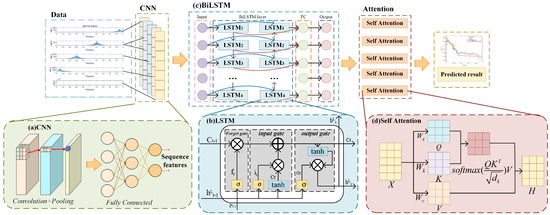
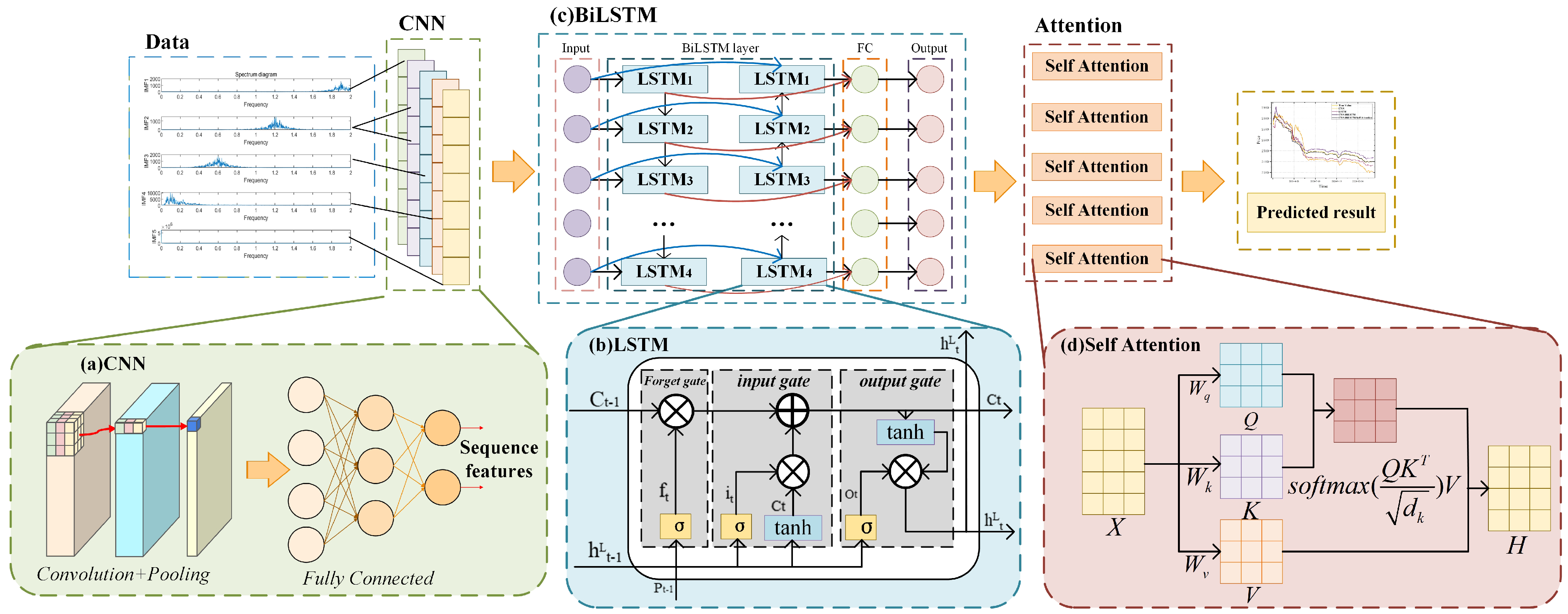
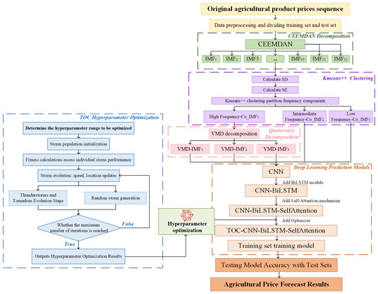
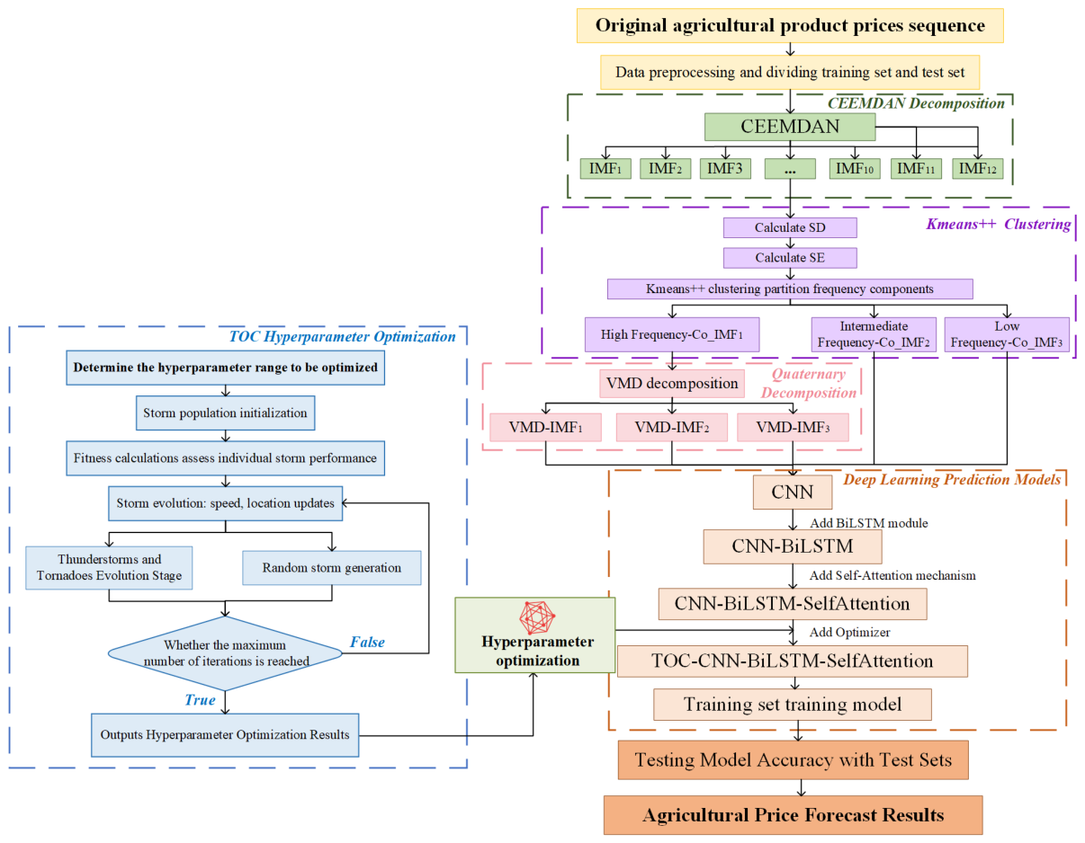
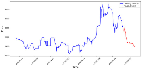
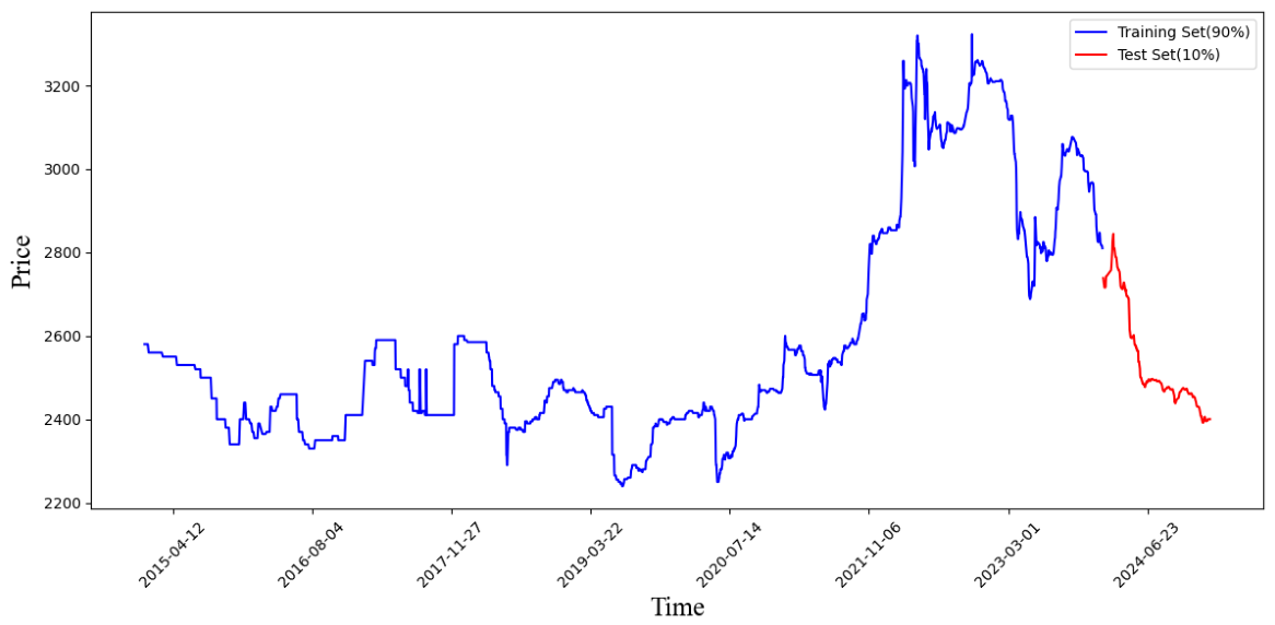
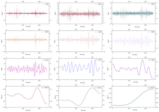
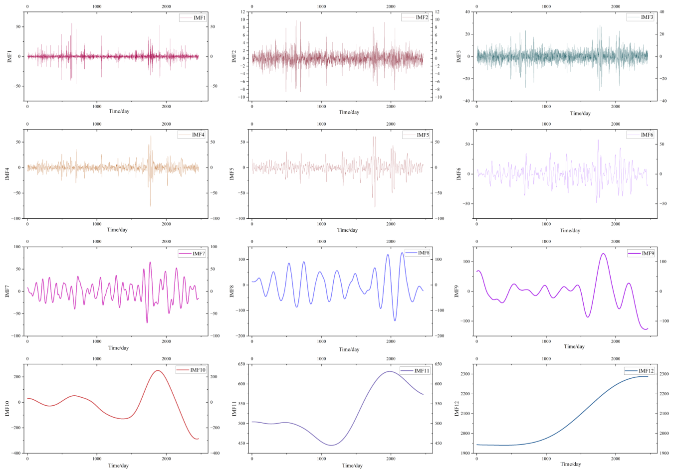
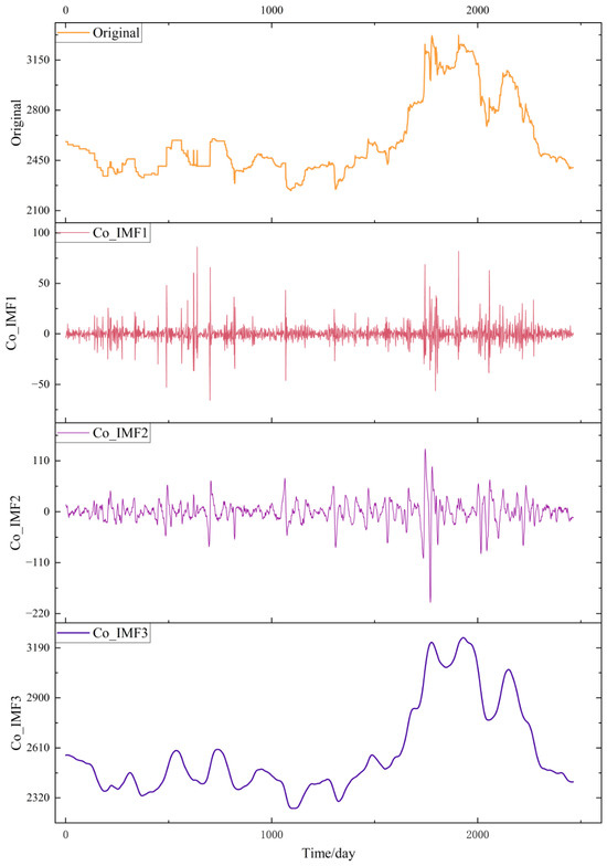
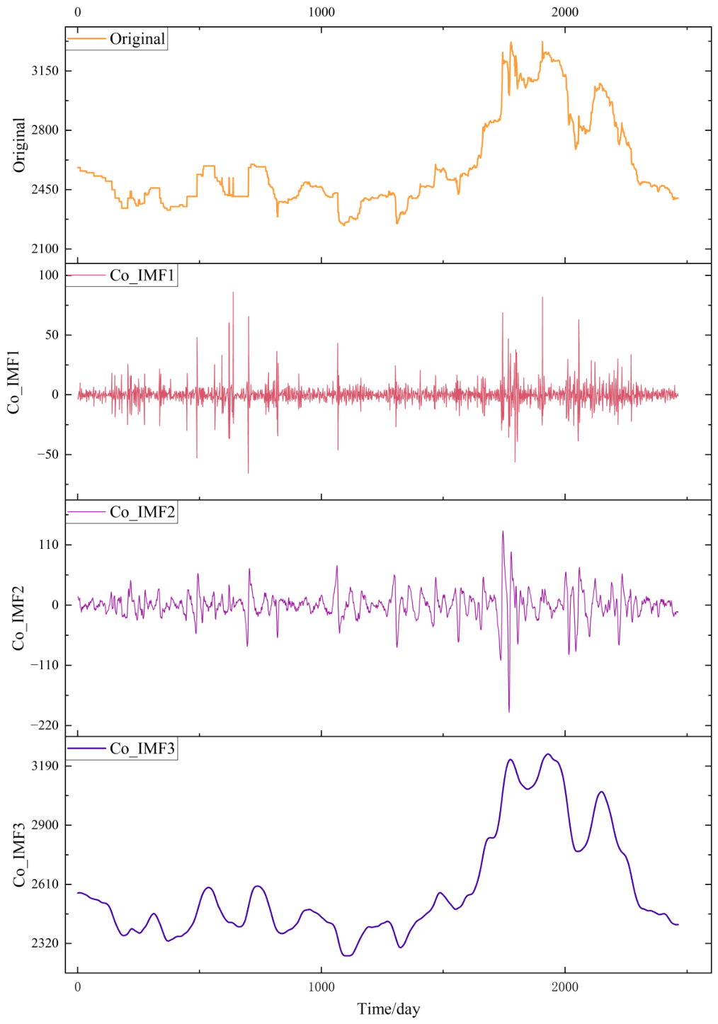
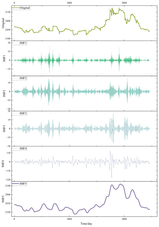
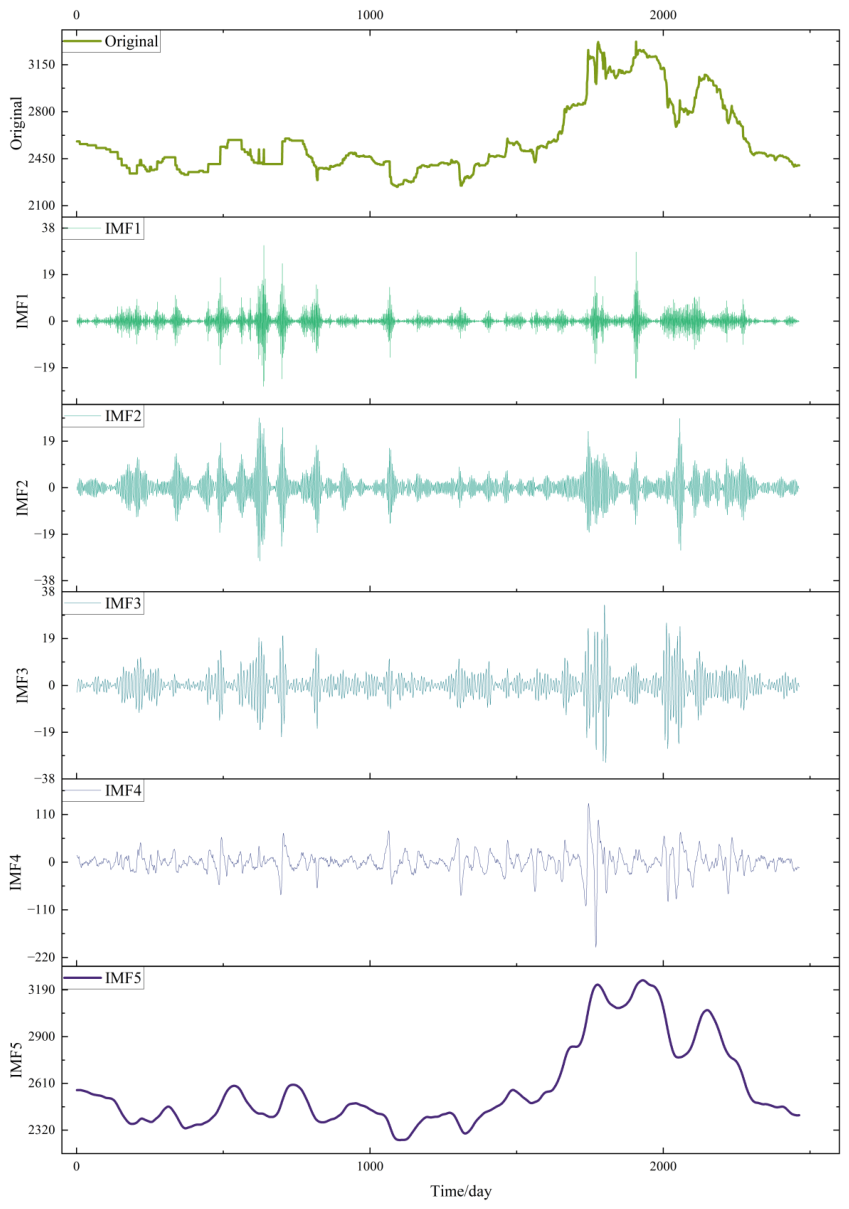
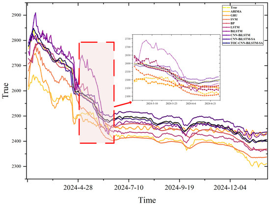
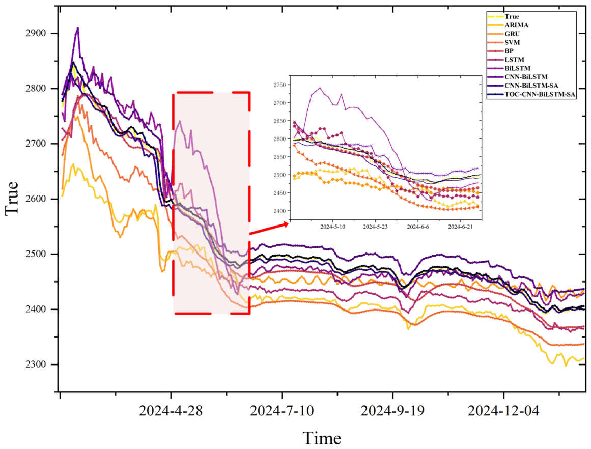
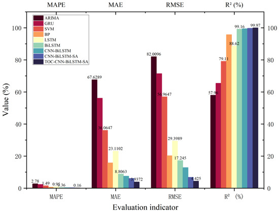
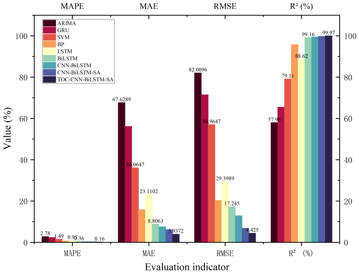
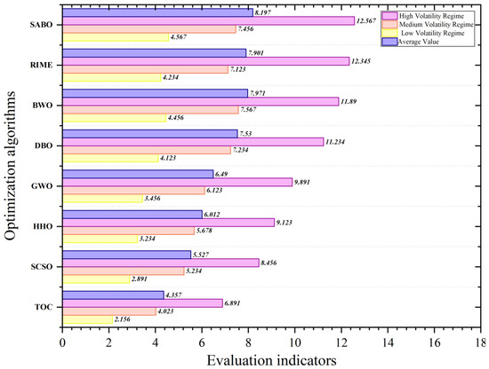
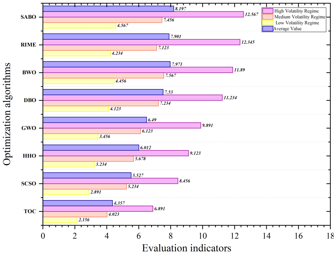
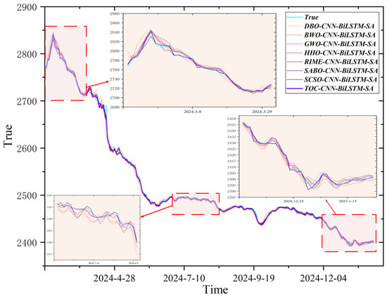
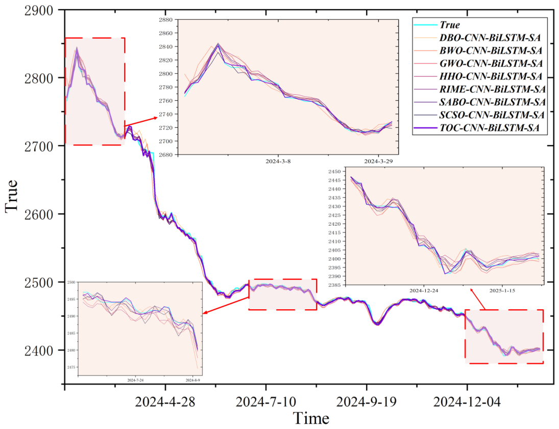
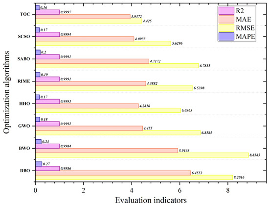
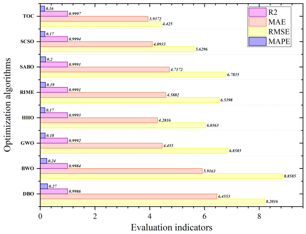
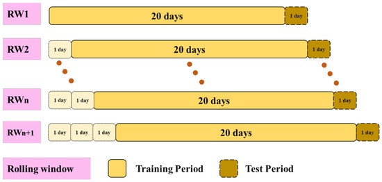
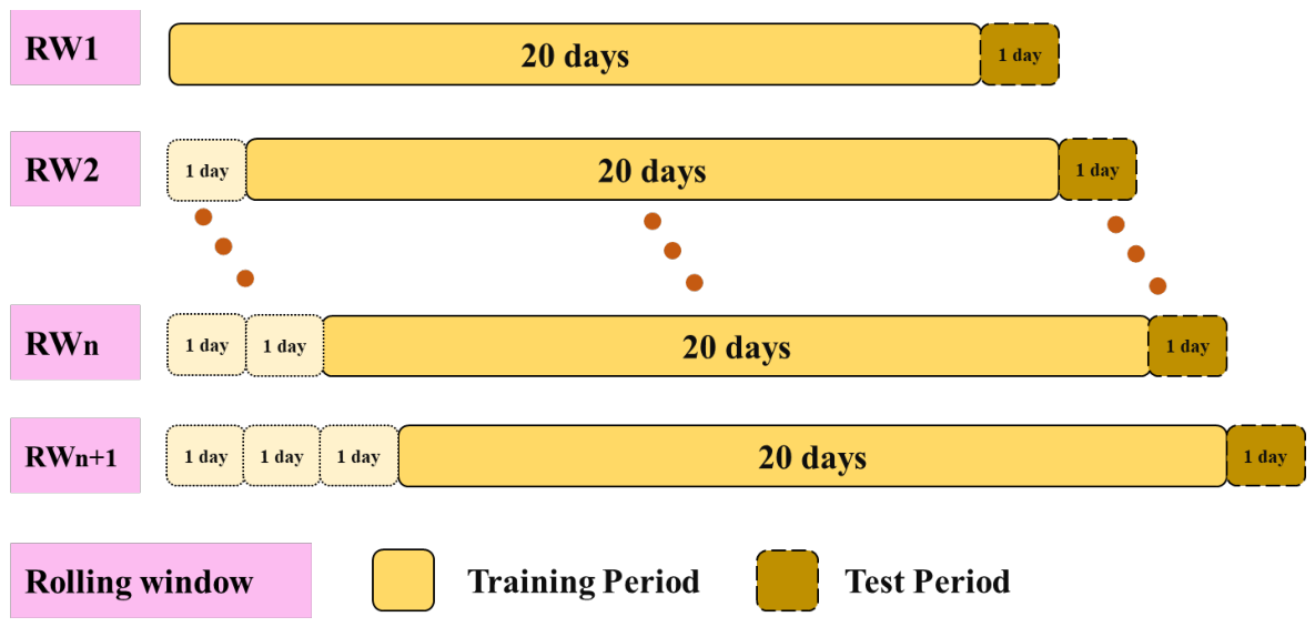
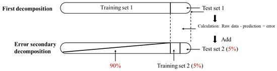
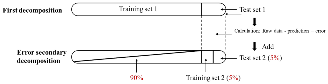
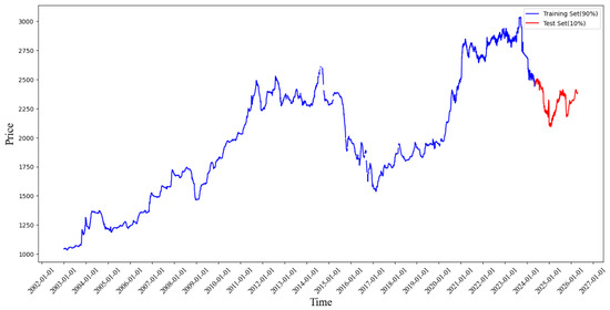
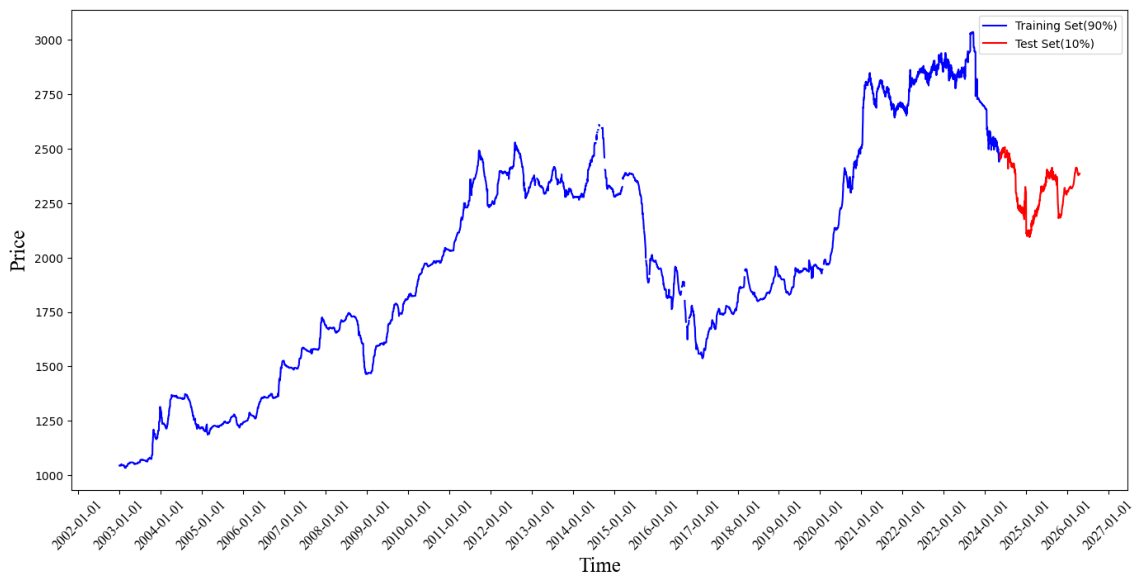
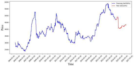
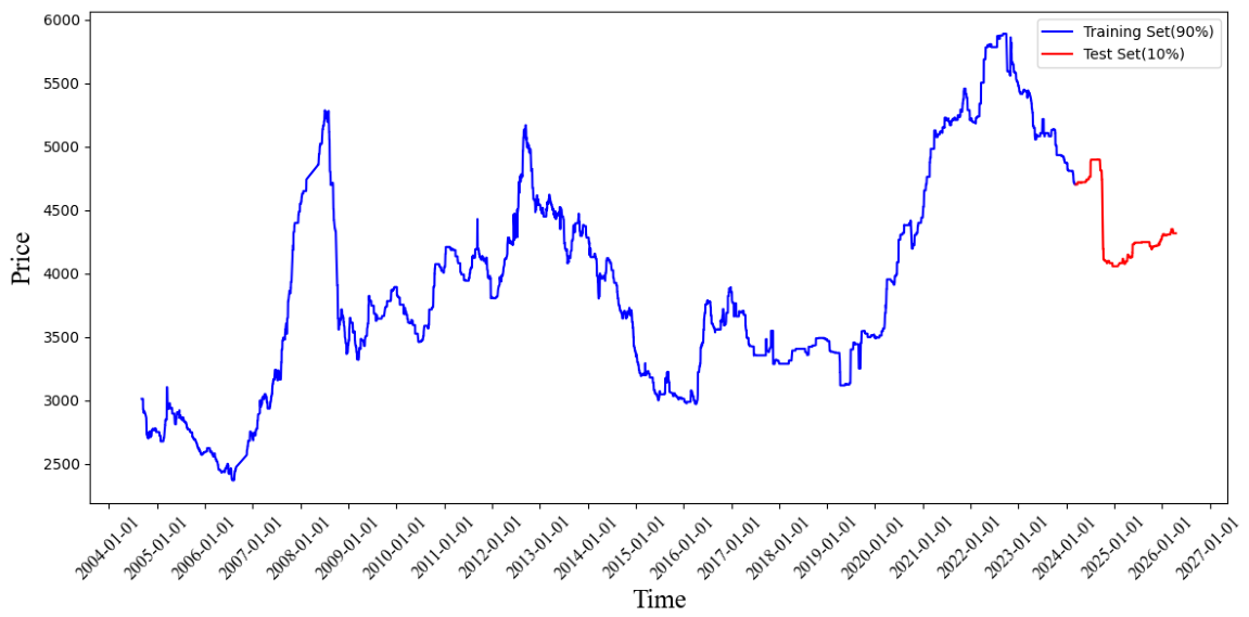

Disclaimer/Publisher’s Note: The statements, opinions and data contained in all publications are solely those of the individual author(s) and contributor(s) and not of MDPI and/or the editor(s). MDPI and/or the editor(s) disclaim responsibility for any injury to people or property resulting from any ideas, methods, instructions or products referred to in the content. |
© 2026 by the authors. Licensee MDPI, Basel, Switzerland. This article is an open access article distributed under the terms and conditions of the Creative Commons Attribution (CC BY) license.