An RMST-Integrated Machine Learning Framework for Interpretable Survival Analysis Under Non-Proportional Hazards: Application to the METABRIC Cohort

Abstract

(1) Background: Advances in machine learning (ML)-based survival modeling enable the analysis of high-dimensional biomedical data. However, many approaches rely on the proportional hazards (PH) assumption, which is frequently violated in oncology and can limit the interpretability of hazard ratio-based results. Using Estrogen Receptor (ER) status in the METABRIC breast cancer cohort as a case study, we propose a framework that integrates machine learning survival models with Restricted Mean Survival Time (RMST) to provide a more robust and clinically interpretable approach for survival analysis under non-proportional hazards. (2) Methods: Overall survival was analyzed in 1104 patients. PH violations were confirmed using Schoenfeld residuals and Kaplan–Meier inspection. We compared four models: stratified Cox Elastic Net (Cox E-Net), Random Survival Forest (RSF), Gradient Boosting Survival Analysis (GBSA), and DeepHit. Performance was assessed using Harrell’s C-index, time-dependent IPCW C-index, and Integrated Brier Score (IBS). RMST at 180 months was utilized to quantify absolute survival differences between ER subgroups. To improve the stability of the estimates, 200 bootstrap resamples were performed, and 95% confidence intervals were derived from the bootstrap distribution. (3) ER status demonstrated significant PH violation (p < 0.005) with crossing survival curves. Discrimination (C-index 0.664–0.725) and calibration (IBS 0.149–0.169) were comparable across models, with RSF achieving the highest overall performance. Despite similar accuracy, survival curve structures differed substantially. Cox E-Net and RSF reproduced the observed crossing pattern, whereas GBSA generated smoother trajectories and DeepHit showed marked compression of subgroup separation. In the independent test cohort, the empirical RMST difference at 180 months was 16.6 months (ER-positive: 130.4; ER-negative: 113.8). Model-based RMST differences ranged from 1 month (DeepHit) to 27 months (Cox E-Net), with RSF and GBSA (12.8 and 13.8 months) most closely approximating the empirical benchmark. (4) Conclusions: We propose a novel, model-agnostic ML + RMST framework that addresses non-proportional hazards while providing quantifiable, time-specific clinical benefit. Moreover, models with similar discrimination and calibration produced markedly different survival curve behavior and absolute RMST estimates, demonstrating that accuracy metrics alone are insufficient for clinical interpretation. By linking prognostic modeling with absolute survival quantification, this framework advances survival evaluation beyond relative risk ranking toward individualized, clinically meaningful decision support.

1. Introduction

Survival analysis is a statistical framework specifically designed to analyze time-to-event data, such as the time until death, disease recurrence, or recovery [1]. It plays a vital role in clinical research across fields like oncology [2,3], cardiology [4], and infectious diseases [5], where understanding the timing and likelihood of events is essential. Among its established methodologies, the Cox proportional hazards (PH) model has long been a foundational tool, widely favored for its semi-parametric flexibility and intuitive interpretability [6,7]. The model expresses the hazard function at time t as:

$$h\left(t,X\right)=h_0\left(t\right)\mathrm{e}\mathrm{x}\mathrm{p}({\beta }_1{x}_1+{\beta }_2{x}_2+\dots {\beta }_p{x}_p)$$

In this formula, $h(t,X)$ is the hazard rate for an individual with a specific set of covariates X, and $h_0(t)$ is the baseline hazard function, which is unspecified and common to all individuals, making the model semi-parametric [8]. The exponentiated term captures the multiplicative effect of covariates on the hazard, allowing for intuitive interpretation via hazard ratios. $\beta$ is the vector of regression coefficients, which quantify the effect of each predictor variable on the hazard. This formulation’s primary advantage lies in not requiring explicit specification of $h_0(t)$, making it highly adaptable to a wide range of datasets [7,9].

However, a key limitation of Cox model is its reliance on a critical proportional assumption: that the hazard ratio between groups remains constant over the entire study period [6,7,9,10]. This “proportional hazards” assumption is frequently violated in real-world clinical datasets [11,12]. Such violations can arise from evolving treatment effects, changes in disease progression, or shifts in patient behavior, causing hazard ratios to vary across the follow-up period and thereby weakening both the reliability and interpretability of the model [13]. These violations are especially problematic for clinically important covariates. For example, the study [14] analyzed 2873 primary breast cancer patients and found that ER-positive status initially conferred protection (HR < 1.0) but later conferred risk (HR > 1.0), indicating time-varying effects. Similarly, the breast cancer study observed that factors like menopausal status and tumor size exhibited non-proportional effects across follow-up period in 3922 breast cancer cases, meaning their hazard ratios changed over the follow-up period rather than remaining constant [15].

Despite these well-documented limitations, the Cox model remains widely used in practice, often without a formal assessment of the PH assumption. A review of 112 studies employing multivariable Cox regression found that violations of the PH assumption were rarely tested or reported, raising concerns about the validity of inferential conclusions [16]. In response, investigators frequently adopt hybrid strategies that pair Cox regression with Kaplan–Meier (KM) curves to supplement inference with visual assessment of survival differences [17]. While KM curves are intuitive and effective for displaying cumulative survival probabilities and comparing groups [18], they require categorization of predictors and cannot adjust for continuous covariates [19]. As a result, KM-based interpretations may be misleading when hazard functions differ over time or when covariate effects are inherently time-dependent [20].

To better accommodate non-proportional hazards, several statistical extensions of the Cox model have been developed. One widely used method is the stratified Cox model, which allows separate baseline hazard functions for strata defined by covariates that do not satisfy the proportional hazards assumption [12,21]. By stratifying on these covariates, their effects are absorbed into stratum-specific baseline hazards rather than being modeled through a single hazard ratio. A key limitation is that the effect of the stratified covariate cannot be directly quantified within this framework. Additionally, stratification can reduce statistical power, especially when strata contain few events [22].

Another traditional solution is the time-dependent Cox model, in which the covariate’s effect is allowed to vary over time or interact with a function of time (e.g., log(time) or time itself) [23]. This method involves incorporating a time-varying coefficient into the hazard function, such as $h\left(x|X\right)=h_0\left(t\right) exp({\beta }_1{x}_1 + {\beta }_2{x}_2(g(t))$, where $g(t)$ is a function of time. Although more flexible, this model adds considerable complexity. Interpreting time-varying hazard ratios is challenging, especially for non-statistical audiences [10]. Its results are also sensitive to the choice of $g(t)$, and the model’s flexibility can come at the cost of increased difficulty in communication and reproducibility [23].

Similarly, flexible spline-based extensions of the Cox model, such as natural cubic splines, allow hazard ratios to vary smoothly over time and can accommodate non-proportional hazards [24]. While these approaches may improve model fit, they require careful selection of spline parameters, as excessive flexibility can lead to overfitting and reduced generalizability [8,25]. Alternative strategies, such as step-function Cox models that partition follow-up time into discrete intervals with piecewise-constant hazards, have also been used to capture time-dependent effects. For example, breast cancer studies have shown that menopausal status exhibits non-monotonic hazard patterns over time, violating proportional hazards assumptions [15].

Despite their theoretical appeal, all three methods increase model complexity, require additional tuning decisions, and impose a greater computational burden. Importantly, in routine clinical or industrial practice, it is rarely known a priori which covariates will violate the proportional hazards assumption at trial initiation. As a result, such model extensions are not commonly implemented prospectively, limiting their practical applicability in real-world oncology studies.

To address these limitations, the Restricted Mean Survival Time (RMST) has gained increasing attention as a robust, clinically interpretable alternative that does not rely on the proportional hazards assumption. RMST is defined as the area under the survival curve from time zero to a pre-specified time point τ and represents the average event-free survival time within that period. Unlike the hazard ratio, which is a relative measure and does not reflect the absolute survival experience or timing of events, RMST expresses treatment effects directly in units of time, making it easier to interpret clinically [26]. Importantly, similar hazard ratios can mask substantial differences in absolute survival benefit. For example, in an analysis of four MRC cancer trials, hazard ratios were comparable (approximately 0.85), yet the difference in RMST at five years ranged from 0.09 years (~1 month) in the ASTEC trial to 0.29 years (~3.5 months) in the OE02 trial [26]. This variation reflects differences in underlying survival probabilities and highlights that hazard ratios do not translate directly into time gained. In addition, RMST remains valid and interpretable when the proportional hazards assumption is violated. In the OE02 trial, evidence of time-varying treatment effects made the Cox model hazard ratio difficult to interpret, whereas RMST provided a clear summary of treatment benefit, corresponding to an average survival gain of approximately 3.5 months at five years [26]. Overall, RMST offers a transparent and clinically meaningful way to quantify the average survival time gained or lost between treatment groups over a fixed time horizon.

Regulatory bodies such as the FDA and EMA increasingly recognize RMST due to its clarity and practical relevance [27,28]. RMST has been used across multiple disease areas, including oncology, cardiology, and infectious diseases [29], to quantify treatment effects where PH assumptions do not hold. It is regarded as a patient-centered endpoint that translates into actionable clinical benefit. For example, in study [30], RMST was used to evaluate antiretroviral therapy in HIV-infected persons with and without drug use (1.51 years vs. 1.43 years) over a five-year period. Unlike traditional mean survival time, which assumes complete data, RMST avoids extrapolation beyond the last observed event, making it more applicable in censored datasets. RMST can capture meaningful differences even when survival curves separate early and then converge later, a situation in which hazard ratios can be misleading. RMST has also been applied in cardiovascular therapeutics, particularly among older adults with frailty and multiple chronic conditions. In a study of patients undergoing transcatheter aortic valve replacement (TAVR), RMST analysis showed that TAVR patients lived, on average, 12.6 months longer over 5 years than medically treated patients. In contrast, the difference in RMST between TAVR and surgical aortic valve replacement (AVR) was approximately one month over five years and was not statistically significant [31]. This example illustrates that when hazard ratios are difficult to interpret due to time-varying effects or data limitations, RMST provides a robust summary of overall survival benefit without relying on the proportional hazards assumption. Extending these findings to oncology, prior work has demonstrated the practical value of RMST in real-world cancer settings. For example, Ref. [32] reported that patients with liver cancer who received liver transplantation (LT) lived, on average, 12.4 months longer over five years compared with those treated with radiofrequency ablation (RFA). By emphasizing a time-based perspective, RMST enhances clinical decision-making by directly addressing the question of “how much longer” patients are expected to survive.

RMST is robust across a wide range of settings and performs well even when the proportional hazards assumption is satisfied. It does not rely on extrapolation beyond the observed follow-up period and is closely tied to the observed survival data [33]. Several methodological extensions have incorporated RMST into regression frameworks, allowing covariate-adjusted and time-updated comparisons, including pseudo-observation methods and longitudinal RMST models [34]. Despite these advances, RMST-based methods are typically applied in retrospective settings to summarize observed survival experience, rather than to provide forward-looking predictive capability. They primarily provide average survival estimates at the population or subgroup level rather than fully individualized survival trajectories. As a result, RMST alone is limited in its ability to support personalized risk prognostic survival estimation.

The limited ability of RMST to support individualized risk prognostic prediction and to handle high-dimensional data has motivated the rise in machine learning (ML) models in survival analysis. A growing number of methods, such as gradient boosting-based survival models (GBM) [35], Random Survival Forests (RSF) [36], Gradient Boost Survival Analysis [37,38], DeepSurv [39], and DeepHit [40] have been proposed to capture nonlinear relationships and complex interactions that traditional models often miss for high-dimensional data. However, it is a common misconception that all ML-based survival models relax the proportional hazards assumption. For instance, DeepSurv is a neural network extension of the Cox model and therefore still relies on the fundamentals of the proportional hazards framework, despite its ability to model high-dimensional nonlinear features [39]. This constraint limits its utility when dealing with biomarkers that exhibit time-dependent effects.

Despite ML models’ predictive flexibility, they primarily operate at a relative scale level, generate risk scores, but often lack transparency at the biomarker level. As a result, these models do not directly capture the full structure of survival outcomes. In contrast, Survival analysis, involves two fundamental components: the probability of experiencing an event (or censoring) and the timing of that event. When the time dimension is only implicitly modeled, the resulting risk scores can be difficult to interpret in clinically meaningful terms. This gap highlights the need for time-based, interpretable survival measures that more directly support clinical decision-making.

These methodological differences contribute to a broader gap between academic research and industry practice in survival analysis. Academic studies often emphasize predictive accuracy, using metrics such as the concordance index (C-index) [41] and the Brier score [42]. In contrast, industry and regulatory settings primarily rely on retrospective, group-based evaluation tools, including Kaplan–Meier (KM) curves and hazard ratios. This disconnect is further reinforced by a methodological divide between data science and traditional biostatistics, which has limited the clinical adoption of machine learning-based survival models.

Several representative machine learning survival models illustrate the trade-offs between predictive performance, interpretability, and reliance on modeling assumptions. Gradient Boosting Machines (GBM), including CoxBoost and survival-optimized versions of XGBoost and CatBoost, have demonstrated strong performance in complex survival settings [35,43]. Although many GBM implementations rely on a Cox partial likelihood objective and therefore assume proportional hazards, their nonlinear structure allows them to approximate time-dependent effects more flexibly than traditional linear models. However, standard XGBoost frameworks typically output relative risk scores rather than direct estimates of survival probabilities or event times. As a result, they do not natively produce survival functions or Kaplan–Meier style curves, and RMST estimation requires additional modeling steps. Consequently, further methodological integration is needed to translate their strong discriminative performance into clinically interpretable, time-based survival summaries.

Random Survival Forests (RSF), an extension of random forests, have also gained widespread use due to their robustness to overfitting and their ability to capture nonlinear effects and complex interactions [36]. For example, Ref. [36] demonstrated the application of RSF to predict cancer recurrence using data from the SEER breast cancer registry, which included over 1.6 million patients. RSF models provide variable importance measures for factors such as age group, surgery status, and tumor stage, and Kaplan–Meier curves are often used to compare predicted risk groups. While RSF does not mathematically require the proportional hazards assumption, the existing literature rarely evaluates how RSF performance compares with traditional models, particularly in the presence of known PH violations, such as those observed in ER-status biomarkers.

Deep learning-based survival models further extend these ideas. DeepSurv extends the Cox model by replacing the linear predictor with a neural network to capture complex covariate–risk relationships [39]. While DeepSurv has reported improved discrimination compared with classical Cox PH and RSF models (C-index: 0.654 vs. 0.632 and 0.620, respectively), it inherits the Cox model’s proportional hazards assumption and lacks direct Kaplan–Meier-style interpretability. Survival visualization typically requires post hoc stratification, and model performance may be sensitive to parameter tuning.

In contrast, DeepHit directly models the joint distribution of event time and event type, thereby accommodating non-proportional hazards and competing risks without imposing rigid statistical assumptions [40]. On the METABRIC dataset, DeepHit achieved strong discriminative performance, with C-index values ranging from 0.679 to 0.703. These results highlight its effectiveness for population-level risk stratification. However, DeepHit operates largely as a black-box model, providing limited insight into the clinical drivers of its predictions. For example, the influence of established biomarkers such as ER status, HER2, or TP53 on survival timing is not directly interpretable. Although individualized survival curves can be generated, they are not clinically intuitive without additional interpretability tools.

More recently, a novel approach has been proposed that directly models RMST conditional on covariates using a random forest regression framework applied to RMST pseudo-values from the SUCCESS-A breast cancer trial [44]. This method offers a flexible, interpretable alternative to time-to-event analysis, capturing nonlinear effects and covariate interactions while retaining a time-based outcome measure. While the conceptual framework is promising, the study provides limited empirical evidence and lacks a comprehensive comparison with other high-performance survival architectures, such as deep learning. Furthermore, the absence of detailed reporting on standard discriminative metrics, such as the C-index and Brier score, limits a full understanding of its real-world predictive reliability.

Broader methodological gaps are also evident in recent survey studies. Study [45] provided a comprehensive review of machine learning approaches for survival analysis, emphasizing models that relax the proportional hazards assumption, including random survival forests, gradient boosting, and deep learning methods. While the survey thoroughly discusses model architectures, loss functions, and evaluation metrics such as the C-index and Brier score, it places less emphasis on empirical examples and rarely incorporates Kaplan–Meier plots to support clinical interpretation.

Similarly, study [46] reviewed 61 deep learning–based survival models, including Cox-based models like DeepSurv (which predict relative risk scores), ranking-based models, time-to-event distribution models such as DeepHit, and multimodal models using CNNs or RNNs. The paper provides an open-source resource (DL4Survival) for comparing architectures and loss functions and identifies key research gaps such as modeling complex survival settings and standardizing evaluation. Although some studies report risk-group stratification, Kaplan–Meier curves and absolute survival estimates are infrequently emphasized to enhance clinical interpretability. Moreover, study [47] proposed a neural network framework for directly predicting RMST at multiple time horizons using simulated data. While innovative from a methodological standpoint, the focus was primarily on optimizing the DNN-based RMST loss function rather than quantifying clinically interpretable survival differences or absolute benefit between patient subgroups.

This gap highlights a central challenge in survival analysis: interpretable, group-based methods such as RMST provide clear clinical meaning but lack individual-level personalization, while machine learning (ML) models offer personalized predictions but often lack clinical interpretability. Bridging this divide requires a framework that combines the predictive power of ML with time-based survival measures meaningful to clinicians and regulators. This study addresses this need by linking modern ML survival models with RMST-based interpretation, particularly in settings where the proportional hazards assumption is violated.

We apply this framework to the METABRIC breast cancer dataset, focusing on estrogen receptor (ER) status, a clinically important biomarker known to violate the proportional hazards assumption [48,49,50]. First, we calculate RMST directly from the observed data to establish a real-world benchmark for ER-positive and ER-negative patient groups. We then develop several ML-based survival models, including Regularized Stratified Cox Elastic-Net (Cox E-Net), Random Survival Forests (RSF), Gradient Boost Survival Analysis (GBSA), and DeepHit, to generate individualized survival predictions. Group mean RMST values are subsequently derived from the aggregated individual predicted survival curves produced by each model.

Our primary contribution is a dual-metric evaluation framework that assesses both predictive performance and clinical relevance:

• Academic Rigor (Predictive Power): We utilize the C-index, and Brier Score to quantify each model’s discriminative power and calibration [30,42].
• Practical Application (Interpretability): We calculate the group-mean RMST at τ = 180 values derived from individualized model predictions and compare them with the benchmark RMST observed in the original patient groups [26].

This integrated approach ensures that ML models are not only statistically accurate but also produce interpretable, time-based survival estimates that support clinical decision-making and regulatory evaluation. By translating complex ML survival estimation into RMST-based summaries, our framework provides a practical and robust solution for survival analysis in the presence of non-proportional hazards.

2. Materials and Methods

2.1. Data Preprocessing

The Molecular Taxonomy of Breast Cancer International Consortium (METABRIC) dataset includes 2509 patients with multiple time-to-event endpoints. To ensure a consistent and clinically meaningful outcome definition, the analysis focused on Overall Survival (OS), and relapse-related variables were excluded. After removing cases with missing OS information, 1981 patients remained. All censoring in the dataset is right-censoring, directly inherited from the original data without modification; no additional censoring rules or transformations were applied in the modeling process.

Feature preprocessing removed non-informative or redundant variables. Invariant features (e.g., sex and cancer type) were excluded. Estrogen receptor (ER) status determined by immunohistochemistry (IHC) was retained as the reference biomarker, while HER2 status was restricted to clinically validated measurements rather than SNP6-derived variables. To reduce multicollinearity and avoid composite bias, high-level prognostic indices such as the Nottingham Prognostic Index (NPI) and Integrative Cluster classification were excluded, allowing constituent clinical variables (e.g., tumor size and lymph node involvement) to be modeled directly.

The final feature set consisted of 20 publicly available clinical variables commonly used in breast cancer prognosis (Table 1), consistent with prior literature [51]. To emulate a prospective clinical trial setting and ensure comparability across models, a complete-case analysis was performed, resulting in a final analytical cohort of 1104 patients.

Table 1. Clinical feature set and preprocessing pipeline for the complete-case METABRIC cohort (n = 1104).

Variable Type	Variables	Treatment
Continuous (4)	Age at Diagnosis, Lymph nodes examined positive, Mutation Count, Tumor Size	Standard normalize (fit on train only)
Binary (9)	ER Status, PR status, HER2 Status, Chemotherapy, Hormone Therapy, Radio Therapy, Type of Breast Surgery, Inferred Menopausal State, Primary Tumor Laterality	Map to 0/1 via BINARY_MAP
Categorical (7)	Cancer Type Detailed, Cellularity, Pam50+ Claudin-low subtype, Tumor Other Histologic Subtype, 3-Gene classifier subtype, Neoplasm Histologic Grade, Tumor Stage	One-hot encode

Variables were preprocessed according to type to ensure compatibility with machine learning models (Table 1). Continuous variables were standardized using mean–variance scaling based on the training set to prevent data leakage. Binary variables were encoded as indicator variables (0, 1), and multi-class categorical variables were transformed using one-hot encoding.

To address limitations of traditional survival analysis under non-proportional hazards (PH), we implemented a multi-stage analytical framework integrating classical survival diagnostics with machine learning methods [52]. The workflow consisted of three components: (1) evaluation of the PH assumption; (2) comparative assessment of model performance using discrimination and calibration metrics; and (3) estimation of Restricted Mean Survival Time (RMST) to provide clinically interpretable time-based comparisons between ER subgroups.

This framework links traditional population-level survival summaries with modern machine learning based survival estimation models, translating complex model output into interpretable time-based comparisons that are robust to violations of the proportional hazards assumption.

2.2. Restriction Time Horizon (τ)

Given PH violations observed in ER status (Schoenfeld test p < 0.05; crossing KM curves), Restricted Mean Survival Time (RMST) was selected as the primary metric. RMST is defined as the area under the survival curve $S(t)$ up to a prespecified time horizon τ and provides an absolute, clinically interpretable measure of survival time that remains valid under non-proportional hazards [26]. RMST can be interpreted as the average event-free survival time per individual over the specified period, and equivalently as the cumulative survival time across the cohort normalized per patient.

$$RMST\left(\tau \right)={\int }_0^{\tau }S\left(t\right)dt$$

The restriction time horizon was set at τ = 180 months (15 years) to capture long-term survival patterns in breast cancer [53].

2.3. Modeling Architectures

We implemented four Machine learning survival modeling approaches spanning varying levels of flexibility, with the aim of balancing model performance and clinical interpretability. All four models are able to accommodate non-proportional hazard patterns in this study, either inherently through flexible modeling structures (e.g., RSF, GBSA, and DeepHit) or through model adaptation, such as the use of a stratified Cox model.

The following modeling architectures were evaluated:

Stratified Cox Elastic-Net (Cox E-Net): This semi-parametric baseline incorporates L1 (Lasso) and L2 (Ridge) penalties to perform simultaneous feature selection and shrinkage. To address observed violations of the proportional hazards assumption, the model was stratified by Estrogen Receptor (ER) status. This approach allows for subtype-specific baseline hazards, ensuring that the distinct survival trajectories of ER-positive and ER-negative patients [54,55].

Random Survival Forest (RSF): A non-parametric ensemble architecture that extends the Random Forest algorithm to right-censored survival data. RSF captures complex, high-order non-linear interactions by growing multiple decorrelated survival trees and aggregating their cumulative hazard estimates via the Nelson–Aalen estimator. RSF is highly adaptive and does not assume constant risk over time [36].

Gradient Boosting Survival Analysis (GBSA): A non-parametric boosting framework that iteratively optimizes the Cox partial likelihood. GBSA sequentially fits trees to minimize the residual loss of previous iterations. While GBSA utilizes a Cox-based objective function to maintain a stable global risk ranking, its tree-based structure captures high-order feature interactions that traditional linear models omit. This model was included to evaluate whether a stable, high-accuracy risk ranking provides superior clinical utility compared to architecture [37,38].

DeepHit: A discrete-time deep learning architecture designed to learn the joint distribution of event times and survival probabilities directly. DeepHit bypasses traditional hazard-based assumptions by employing a multi-task neural network. The architecture utilizes a combination of two loss functions: one that minimizes the log-likelihood of the first hit (the event), and a second ranking-loss term that specifically encourages correct pair-wise ordering of patients. This allows the model to capture complex, time-dependent relationships and non-proportionality without the constraints of a pre-defined mathematical distribution [40].

Tree-based gradient boosting models (e.g., XGBoost and CatBoost) were not included in this framework, as their commonly used implementations in survival analysis do not directly yield individual survival probability functions, thereby limiting RMST-based interpretation and survival curve estimation.

2.4. Training and Validation Strategy

The analytical cohort (n = 1104) was divided into training (80%) and testing (20%) subsets using multi-label stratification to jointly preserve event status (death vs. censoring) and Estrogen Receptor (ER) subtype distribution. The cohort comprised 107 censored/ER-negative, 142 Event/ER-negative, 382 censored/ER-positive, and 473 Event/ER-positive patients. This Stratification approach ensures the clinical prevalence of biomarker subtypes and outcomes is preserved across both development and evaluation sets.

All survival estimation models were developed using the training set, and performance evaluation was conducted exclusively on the independent test set to ensure unbiased generalization assessment.

Stratified Cox elastic net model: 80 penalty values (α ∈ 10⁻⁴–10¹) were evaluated with l1_ratio = 0.5. Five-fold cross-validation within the training set was used to select the optimal penalty parameter. Separate ER-positive and ER-negative models were fitted to allow subtype-specific baseline hazards.

RSF: use 1000 trees with key parameters of min samples split 10, min samples leaf 5, and max features $\sqrt{p}$. Model performance was evaluated using five-fold cross-validation.

GBSA: use key parameters of learning rate 0.03, n estimators 1000, max depth 3, min samples leaf 15, and subsample 0.8. Model performance was evaluated using five-fold cross-validation.

DeepHit: use an 80/20 train–test split, with five-fold cross-validation within the training set for hyperparameter tuning. The architecture consisted of three fully connected layers with hidden sizes scaled to the number of covariates (3d–5d–3d) and ReLU activation functions, followed by a softmax output layer. Model training used Xavier initialization, dropout (p = 0.6), and the Adam optimizer (learning rate = 1 × 10⁻⁴; batch size = 50). The loss function combined likelihood and ranking components to improve temporal discrimination.

As the focus of this study is ML-RMST framework development rather than predictive optimization, hyperparameters were tuned to achieve reasonable discrimination without extensive optimization. Model performance evaluation was conducted exclusively on the independent test set using a dual method strategy that integrates predictive discrimination with clinical interpretability:

• Model Predictive Performance.

Discrimination was evaluated using Harrell’s concordance index (C-index) and a time-dependent Inverse Probability of Censoring Weighted (IPCW) C-index [41]. Calibration and overall prediction error were assessed using the Integrated Brier Score (IBS) [42].

2.

Clinical Utility and RMST Estimation τ = 180.

Survival estimations were generated for the held-out test cohort (n = 221). For each patient i, individualized Restricted Mean Survival Time (RMST) was calculated up to τ = 180 months by integrating the model-predicted survival function over the specified time horizon.

$$RMS{T}_i\left(\tau \right)={\int }_0^{\tau }\widehat{S}( t\mid x_i) dt$$

Individual-level predictions were generated then aggregated to construct marginalized (population-averaged) survival curves and corresponding mean RMST estimates. The empirical KM curve derived from the full cohort (n = 1104) was used as a high-stability descriptive reference. However, all quantitative model comparisons, including RMST estimation and performance evaluation, were conducted exclusively on the held-out test set (n = 221) to ensure unbiased assessment and equal footing across models.

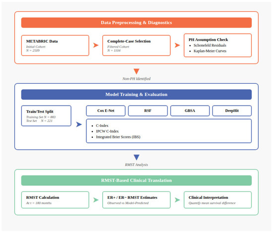
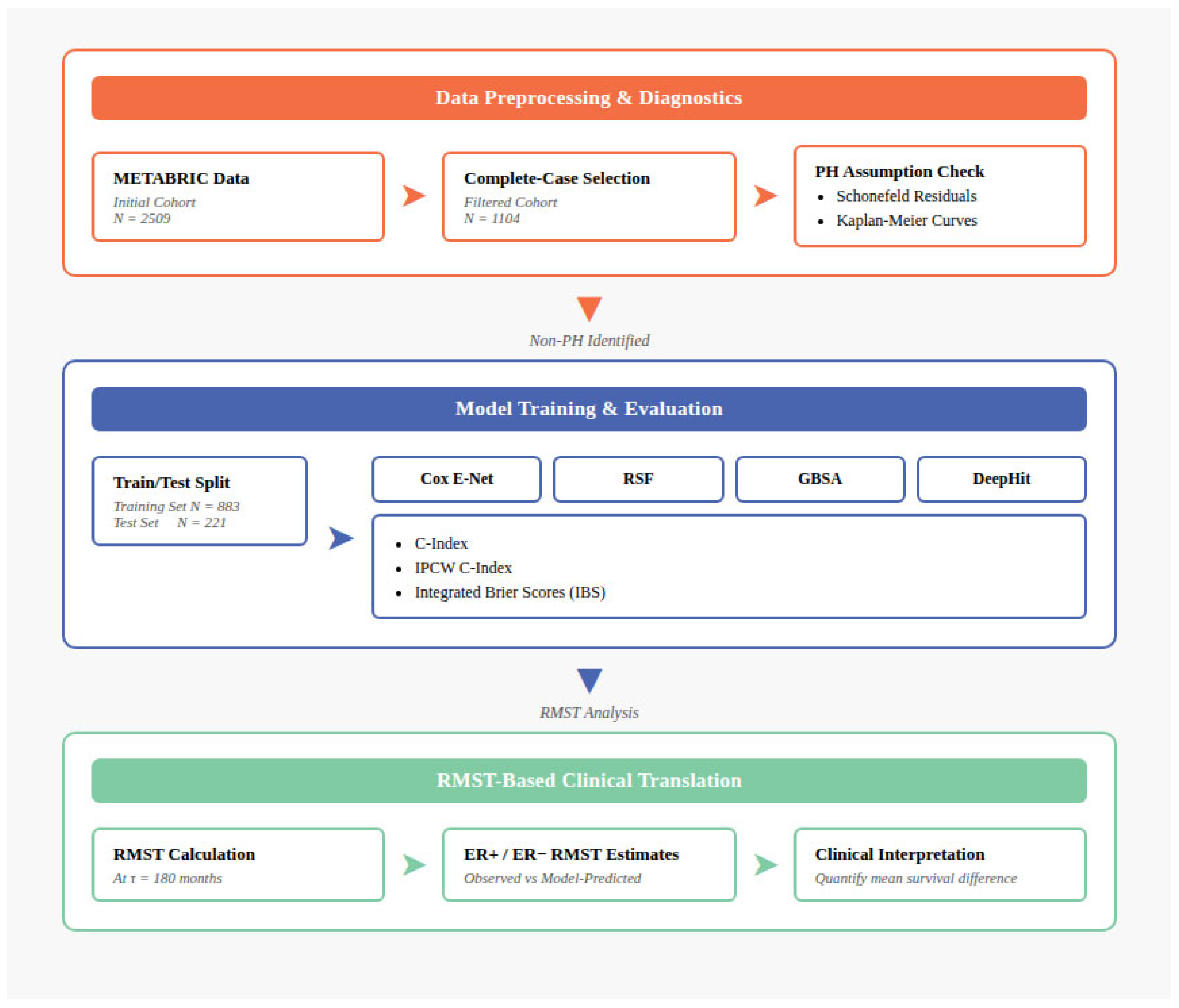
To quantify sampling variability of model-based survival estimates, bootstrap resampling (B = 200 iterations) was performed at the patient level within the held-out test set. Specifically, after generating survival predictions for each individual test subject (n = 221), we repeatedly sampled patients with replacement to create new datasets. For each resampled dataset, the individual predicted survival curves were averaged to obtain a population-level survival curve, and the corresponding RMST was recalculated. This approach preserves subject-level variability and avoids additional model refitting, thereby providing an unbiased assessment of uncertainty conditional on the trained models. The percentile method was used to derive 95% CIs, providing a non-parametric assessment of the stability of the predicted survival probabilities and RMST estimates. All analyses were conducted in Python (version 3.9) using the scikit-survival, scikit-learn, and lifelines libraries [56,57,58]. The overall methodological framework is illustrated in Figure 1.

Figure 1. Study design: PH diagnostics, model training/testing, and RMST-based clinical translation framework. Note. The METABRIC dataset (n = 2509) underwent preprocessing and proportional hazards (PH) diagnostics, followed by train/test splitting (n = 1104). Four machine learning models (Cox Elastic Net, Random Survival Forest, GBSA, and DeepHit) were developed and evaluated in the independent test cohort (n = 221) using discrimination and calibration metrics. Clinical translation was achieved through Restricted Mean Survival Time (RMST) estimation at 180 months, comparing model-based and observed ER subgroup survival differences and survival curve patterns.

3. Results

3.1. Assessment of the Proportional Hazard Assumption

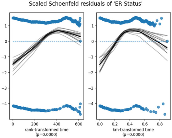
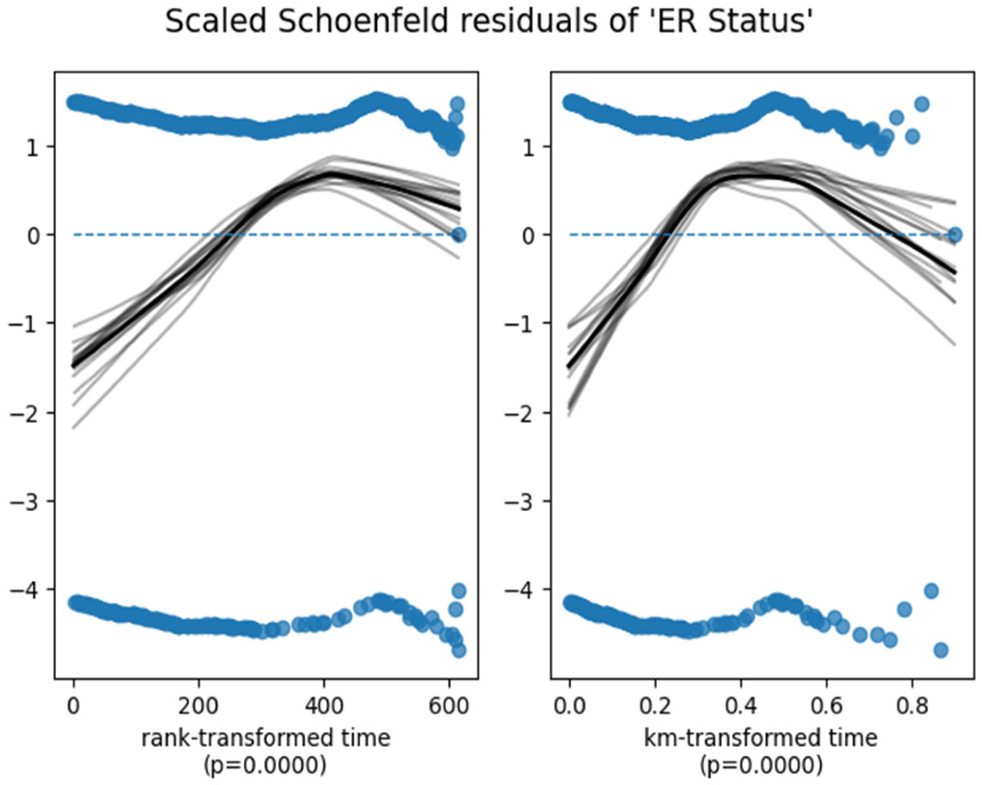
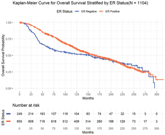
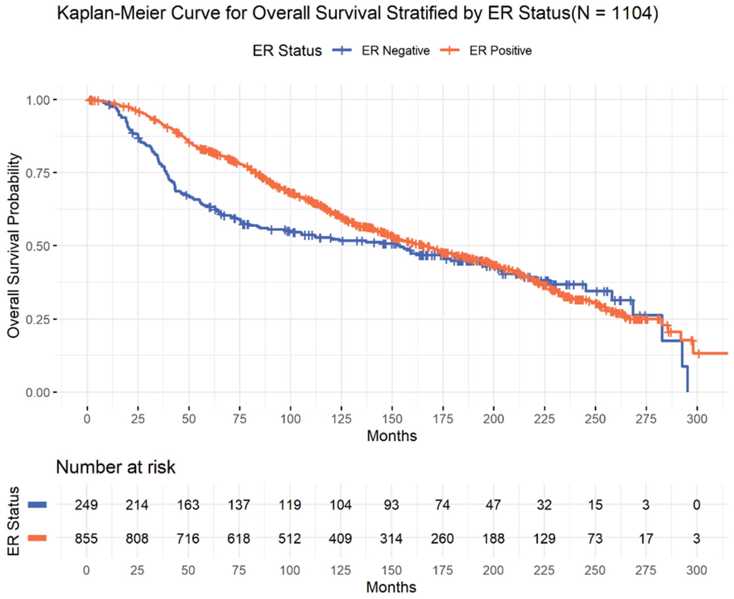
To assess the proportional hazards (PH) assumption for estrogen receptor (ER) status, a Cox proportional hazards model was fitted using CoxPHFitter, and Schoenfeld residual diagnostics were evaluated in the full cohort (n = 1104). The global test based on scaled Schoenfeld residuals demonstrated significant violation of the PH assumption (p < 0.005), with test statistics of 32.21 (KM-transformed test) and 41.21 (rank-transformed test), indicating strong evidence of time-varying effects. The scaled Schoenfeld residual plots showed systematic deviation from zero over time (Figure 2). Consistently, Kaplan–Meier curves for ER-positive and ER-negative patients crossed during follow-up (Figure 3), further supporting the presence of non-proportional hazards.

Figure 2. Scaled Schoenfeld residuals for ER status from the Cox model. Note. The smoothed trend lines deviate from zero over time in both rank-transformed and Kaplan–Meier-transformed scales, indicating violation of the proportional hazards assumption (global test p < 0.001).

Figure 3. Kaplan–Meier curves for overall survival stratified by estrogen receptor (ER) status (n = 1104). Note. ER-positive patients demonstrate improved early survival; however, the curves converge and cross during long-term follow-up, indicating violation of the proportional hazards assumption. Tick marks represent censored observations. Numbers at risk are shown below the plot.

These results suggest that the effect of ER status on overall survival is not constant over time, thereby motivating the use of alternative modeling strategies and time-based summary measures such as RMST.

3.2. Predictive Model Performance

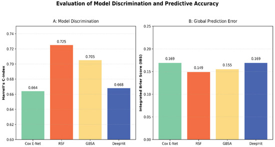
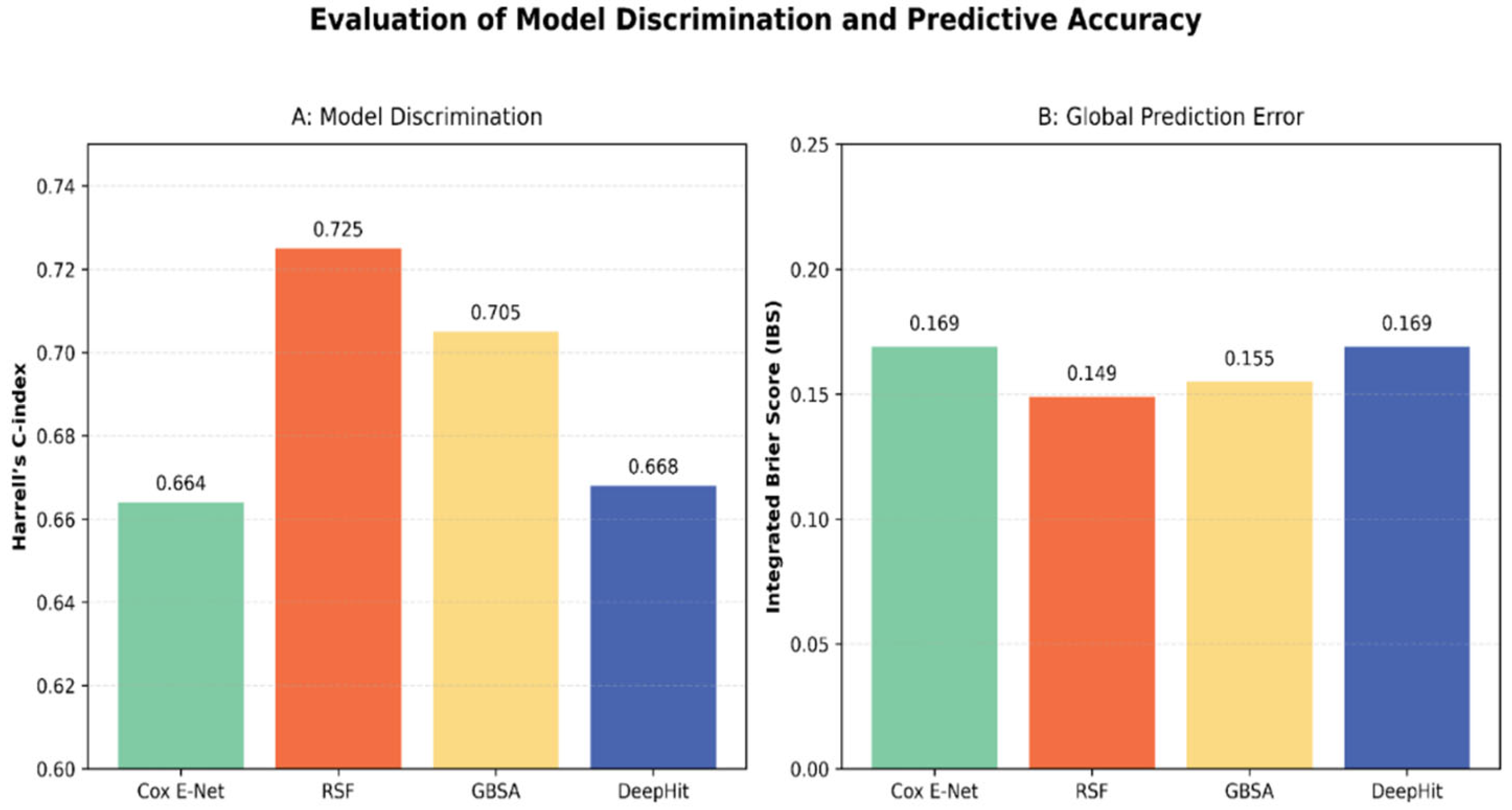
Model discrimination was evaluated on the independent test cohort (n = 221), which included 49 ER-negative patients (21 censored, 28 events) and 172 ER-positive patients (77 censored, 95 events). Discriminatory performance was assessed using Harrell’s concordance index (C-index), which measures the ability of a model to correctly rank survival times among comparable patient pairs. The overall (static) C-index values were 0.664 for Cox-ENet, 0.725 for RSF, 0.705 for GBSA, and 0.668 for DeepHit (Figure 4A). Among the evaluated models, RSF achieved the highest discrimination.

Figure 4. Predictive performance on the independent test set: Discrimination (C-index) and Overall Error (IBS). Note. (A) Model discrimination assessed using Harrell’s C-index, where higher values indicate improved ability to correctly rank survival times. (B) Global predictive accuracy evaluated using the Integrated Brier Score (IBS), where lower values reflect better agreement between predicted survival probabilities and observed outcomes. Across both metrics, RSF demonstrated the strongest overall performance. Abbreviations: Cox E-Net, Stratified Cox Elastic Net, RSF, Random Survival Forest; GBSA, Gradient Boosting Survival Analysis; IBS, Integrated Brier Score.

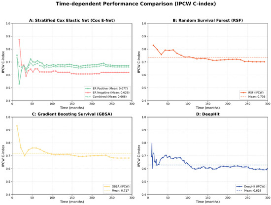
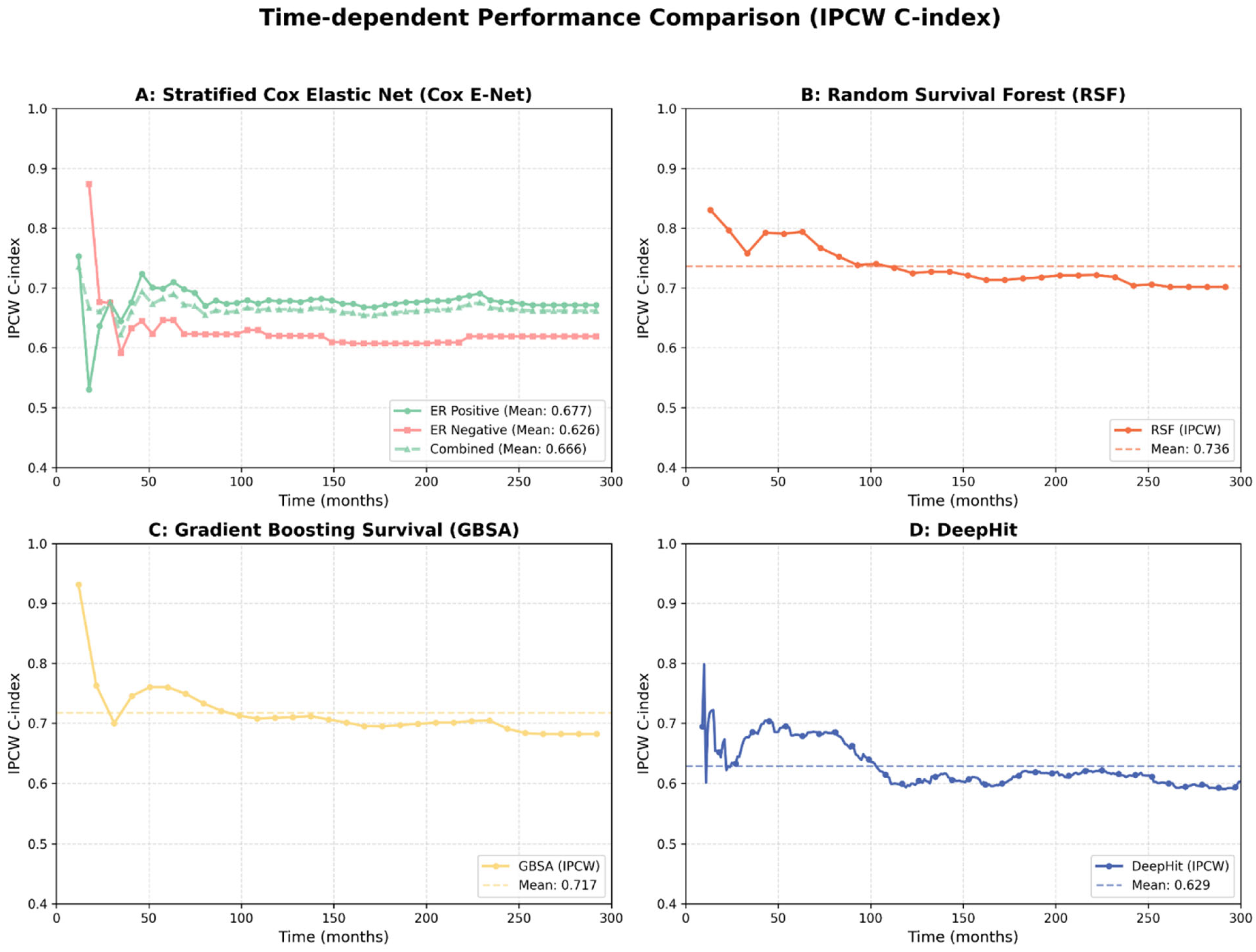
To assess temporal stability of predictive performance, discrimination was further evaluated using the time-dependent Inverse Probability of Censoring Weighted (IPCW) C-index. Unlike the static C-index, which aggregates concordance across the entire follow-up duration, the IPCW C-index evaluates discrimination at prespecified time points while adjusting for censoring. IPCW estimates were computed at approximately 30 time points distributed across the observed follow-up window, and mean IPCW values were reported. For the stratified Cox elastic net model, the mean IPCW C-index was 0.677 for ER-positive patients and 0.626 for ER-negative patients, yielding a combined mean of 0.666, slightly higher than the static estimate (0.664). Similarly, RSF achieved a mean IPCW C-index of 0.736 compared to its static C-index of 0.725, while GBSA demonstrated 0.717 versus 0.705, DeepHit achieved a mean IPCW C-index of 0.629 compared to a slightly higher static C-index of 0.668 (Figure 4) [39,40,59,60].

Across most models, the IPCW C-index was modestly higher than the static C-index (Figure 5). This difference likely reflects the fact that the static C-index incorporates late follow-up intervals with substantial censoring, where discrimination becomes inherently more challenging. In contrast, the IPCW approach reweighs observations to account for censoring and emphasizes time intervals with adequate event information. For DeepHit, the higher static C-index relative to the IPCW estimate likely reflects its multi-task objective function, which prioritizes the global ordering of event times rather than localized hazard estimation at specific time points. Importantly, both static and time-dependent metrics yielded consistent model ranking, with RSF demonstrating the strongest overall discrimination. These values are consistent with ranges reported in prior breast cancer survival modeling studies [39,40].

Figure 5. Time-dependent discrimination (IPCW C-index) across follow-up by model (test set). Note. (A) Cox E-Net performance for ER-positive (mean: 0.677), ER-negative (mean: 0.626), and combined (mean: 0.666). (B) RSF, (C) GBSA, and (D) DeepHit model performances. Mean values for panels (B–D) are represented by horizontal dashed lines. IPCW: Inverse Probability of Censoring Weighting; ER: Estrogen Receptor.

To complement discrimination metrics, we evaluated model calibration and predictive accuracy using two complementary measures: the static Integrated Brier Score (IBS) and time-dependent IPCW Brier curves. The Brier score measures the squared difference between predicted survival probabilities and observed outcomes at specific time points, while the IBS summarizes this error across the entire follow-up period. Lower values indicate superior calibration, with 0.25 serving as the benchmark for a non-informative model [42].

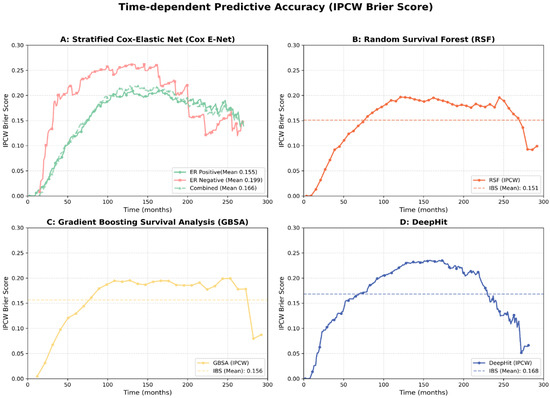
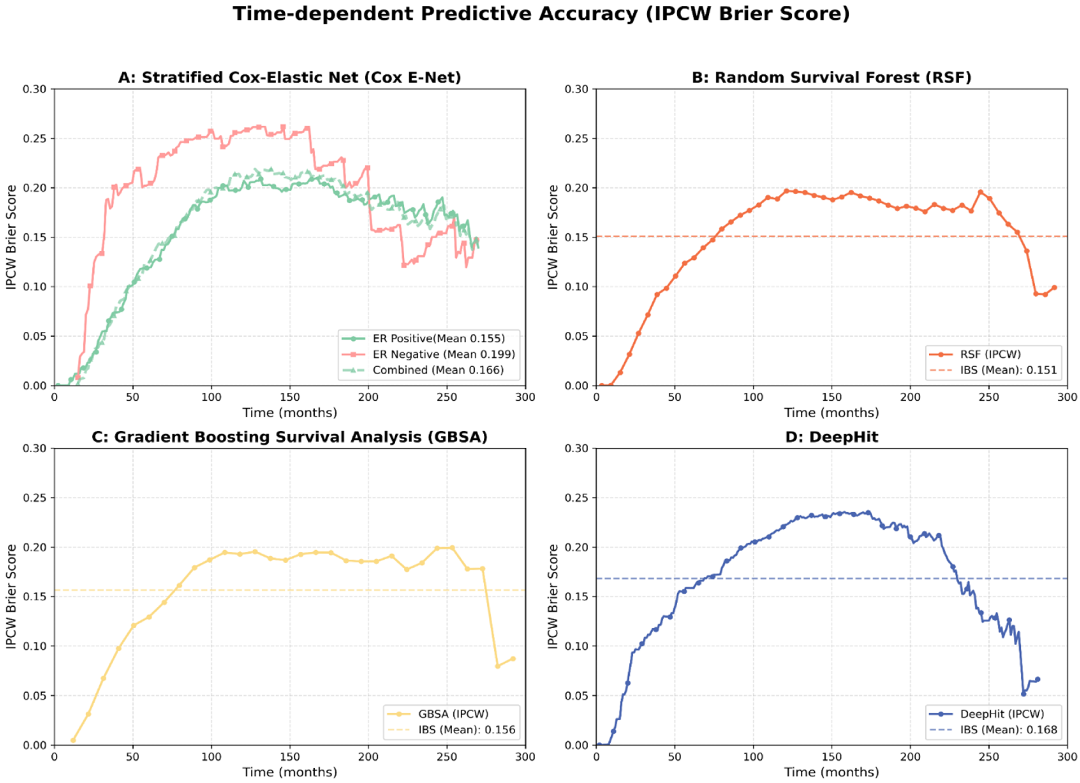
All evaluated architectures performed substantially better than the non-informative baseline, achieving error rates consistent with established breast cancer survival benchmarks [61]. RSF demonstrated the highest overall calibration (IBS = 0.149; Mean IPCW Brier = 0.151), followed closely by GBSA (IBS = 0.155; Mean IPCW Brier = 0.156), while DeepHit (IBS = 0.169; Mean IPCW Brier = 0.168) and the Cox E-Net exhibited slightly higher overall error (IBS = 0.169; Mean IPCW Brier = 0.166) (Figure 4B and Figure 6).

Figure 6. Time-dependent prediction error (IPCW Brier Score) across follow-up by model (test set). Note. Markers indicate performance evaluation at approximately 10-month intervals. (A) Cox E-Net performance for ER-positive (mean: 0.155), ER-negative (mean: 0.199), and combined (mean: 0.166) cohorts. (B) RSF (mean IBS: 0.151), (C) GBSA (mean IBS: 0.156), and (D) DeepHit (mean IBS: 0.168). Solid lines represent instantaneous error; dashed lines indicate the mean Integrated Brier Score (IBS). IPCW: Inverse Probability of Censoring Weighting; ER: Estrogen Receptor.

Subgroup analysis of the Stratified Cox-Elastic Net model (Figure 6A) revealed significant performance heterogeneity; prediction error was markedly higher in the ER-negative subgroup (IBS = 0.199) compared to the ER-positive subgroup (IBS = 0.155). This finding, alongside the lower C-index observed in ER-negative patients, suggests that the increased biological aggressiveness and heterogeneity of the ER-negative subtype present a greater challenge for precise long-term calibration.

Importantly, the time-dependent IPCW Brier curves (Figure 6) were highly consistent with the overall IBS rankings. The error trajectories revealed that predictive inaccuracy generally peaked between 100 and 200 months, the period of highest cumulative event density, before declining in later follow-up as the cohort stabilized. Notably, the ensemble methods (RSF and GBSA) exhibited smoother error trajectories and maintained lower peak errors than the Cox E-Net and DeepHit models. The absence of late-time error inflation across all architectures confirms that the models maintain sustained calibration performance even through the long-term follow-up period.

3.3. Restricted Mean Survival Time (RMST) Estimation

While discrimination metrics such as the C-index and Brier score quantify predictive accuracy, they do not directly translate into clinically interpretable survival differences. To provide an absolute measure of survival benefit between ER subgroups, Restricted Mean Survival Time (RMST) was evaluated up to a horizon of τ = 180 months (15 years).

In the full cohort (n = 1104), the empirical RMST at 180 months was 131.4 months (95% CI: 127.5–135.3) for ER-positive patients and 113.3 months (95% CI: 104.5–122.0) for ER-negative patients. These estimates serve as a stable population-level reference derived from the largest available sample.

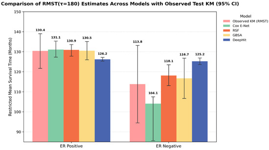
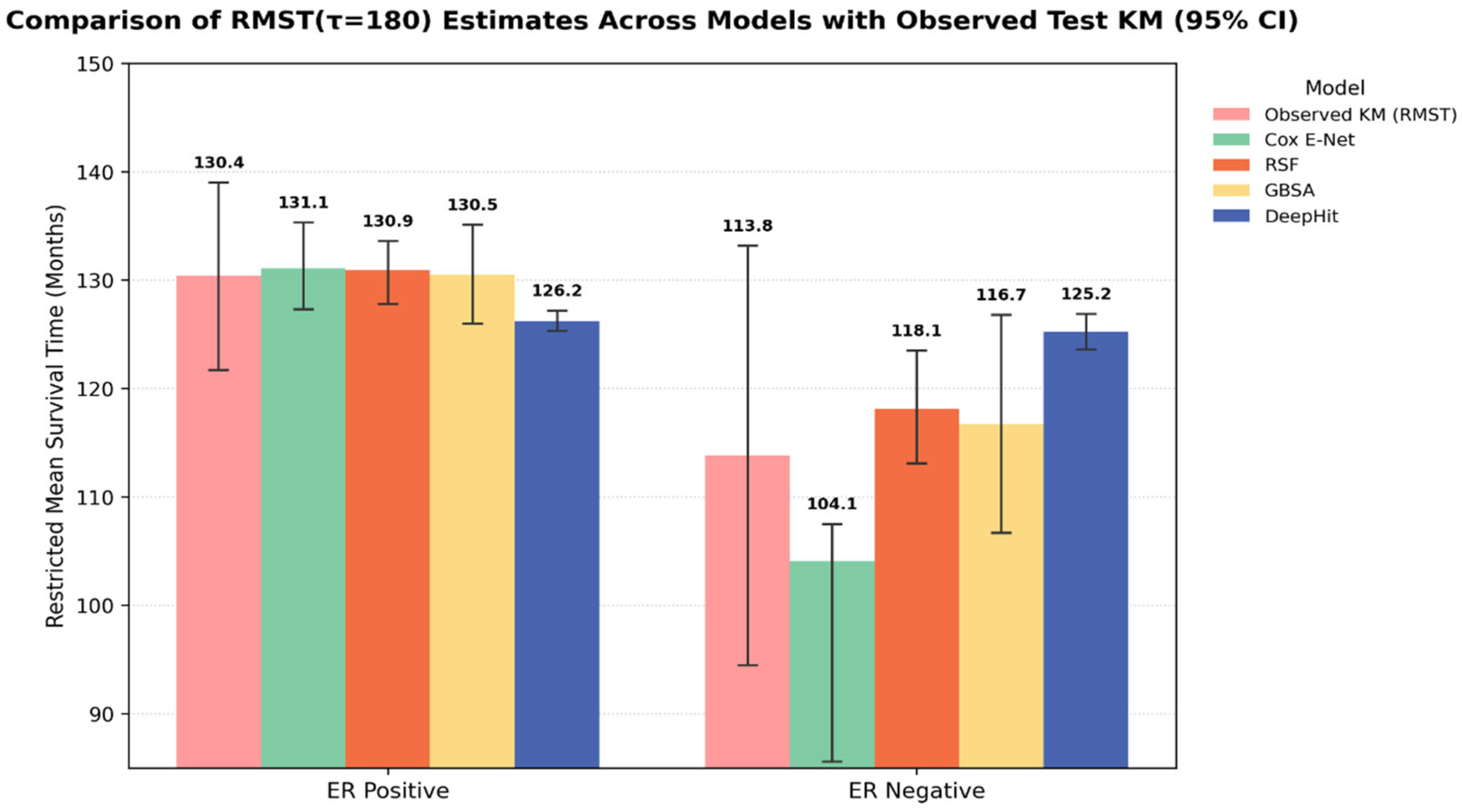
For unbiased model evaluation, all comparative RMST analyses were conducted exclusively in the independent test cohort (n = 221). Empirical Kaplan–Meier estimates in the test set yielded a benchmark RMST at 180 months of 130.4 months for ER-positive patients and 113.8 months for ER-negative patients, corresponding to an absolute survival difference of 16.6 months (Figure 7; Table 2).

Figure 7. RMST at τ = 180 months by ER Status: Observed KM benchmark vs. model-based estimates (test set). Note. Estimates are stratified by ER status and benchmarked against observed Kaplan–Meier (KM) RMST values. Error bars represent the 95% Confidence Interval (CI). Abbreviations: Cox E-Net, Stratified Cox Elastic Net, RSF, Random Survival Forest; GBSA, Gradient Boosting Survival Analysis; ER, Estrogen Receptor.

Table 2. Observed and model-predicted RMST at τ = 180 by ER Subtype in the independent test cohort (n = 221).

Model	ER Positive RMST (95% CI) (Months)	ER Negative RMST (95% CI) (Months)	ER Positive–ER Negative Difference (Months)
Observed KM (Test)	130.4 [121.7–139.0]	113.8 [94.4–133.2]	16.6
Cox E-Net	131.1 [127.3–135.3]	104.1 [85.6–107.5]	27
RSF	130.9 [127.8–133.6]	118.1 [113.1–123.5]	12.8
GBSA	130.5 [126.0–135.1]	116.7 [106.7–126.8]	13.8
DeepHit	126.2 [125.3–127.2]	125.2 [123.6–126.9]	1

Note. Absolute differences quantify ER subgroup (ER positive–ER negative) survival separation across models.

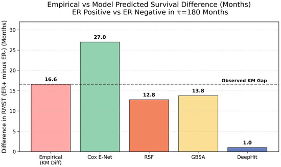
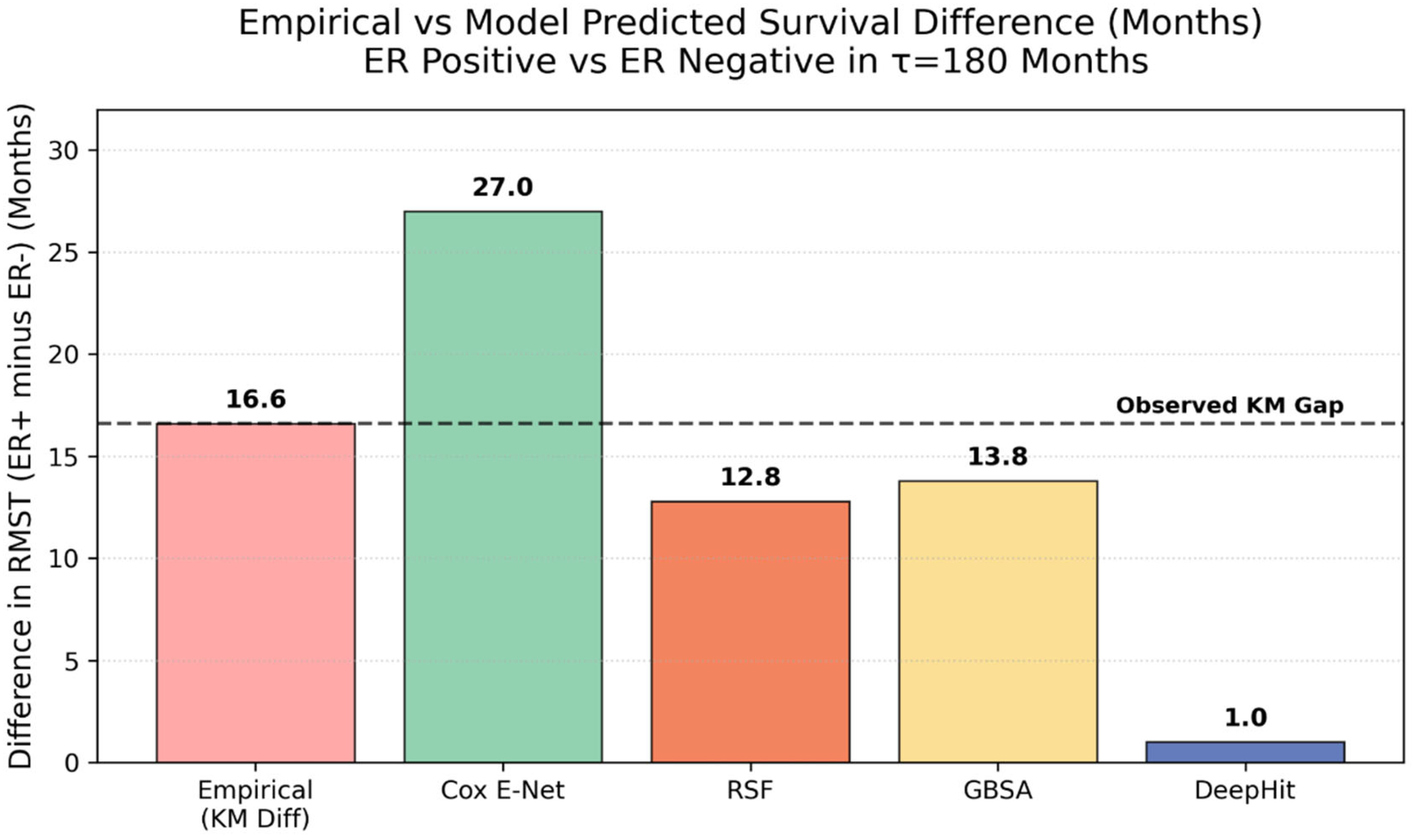
Model-based RMST estimates are summarized in Table 2. Stratified Cox Elastic Net (Cox E-Net) amplified the subgroup separation, producing a 27-month ER difference, exceeding the empirical benchmark. In contrast, Random Survival Forest (RSF) generated a 12.8-month difference that closely approximated the observed survival gap, reflecting the most balanced calibration among evaluated models. Gradient Boosting Survival Analysis (GBSA) yielded the closest subgroup separation (13.8 months), though with wider uncertainty intervals compared to RSF. DeepHit, however, produced markedly compressed RMST estimates between ER groups, resulting in minimal subgroup differentiation and suggesting shrinkage toward the population mean.

Across models, RMST estimates for ER-positive patients were consistently close to the empirical benchmark 130.4 months (range: 126.2–131.1 months), indicating stable long-term survival prediction in this subgroup. In contrast, substantially greater variability was observed for ER-negative patients (range: 104.1–125.2 months) relative to the 113.8-month empirical mean. This heterogeneity likely reflects both the more aggressive clinical trajectory and earlier concentration of events characteristic of ER-negative disease, which increases sensitivity to time-varying effects and violations of the proportional hazards assumption. Additionally, the smaller ER-negative sample size may further amplify estimation instability across model architectures.

Importantly, all evaluated models correctly identified the survival advantage for ER-positive patients and provided a quantified estimate of the absolute time benefit at τ = 180 months (Figure 8). However, the magnitude of this gain varied significantly. These RMST findings also complement the discrimination and calibration results. Cox E-Net amplified subgroup separation primarily due to underestimation of ER-negative survival, consistent with its comparatively weaker C-index and IBS in the subgroup. In contrast, RSF (12.8 months) and GBSA (13.8 months) achieved strong C-index and Brier performance while also producing RMST differences closest to the empirical benchmark (16.6 months), suggesting more balanced modeling of time-varying survival dynamics. DeepHit, despite competitive discrimination, substantially attenuated the survival gap (1 month), underscoring that similar ranking performance does not guarantee accurate estimation of clinically relevant survival differences.

Figure 8. Comparison of empirical and model-predicted RMST differences (ER-positive minus ER-negative) at τ = 180 months. Note. The dashed line represents the observed Kaplan–Meier (KM) RMST difference (16.6 months) in the test cohort. While Cox-ENet amplified the survival gap and DeepHit markedly compressed it, RSF and GBSA produced estimates closer to the empirical benchmark. Abbreviations: Cox E-Net, Stratified Cox Elastic Net, RSF, Random Survival Forest; GBSA, Gradient Boosting Survival Analysis; ER, Estrogen Receptor.

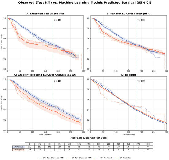
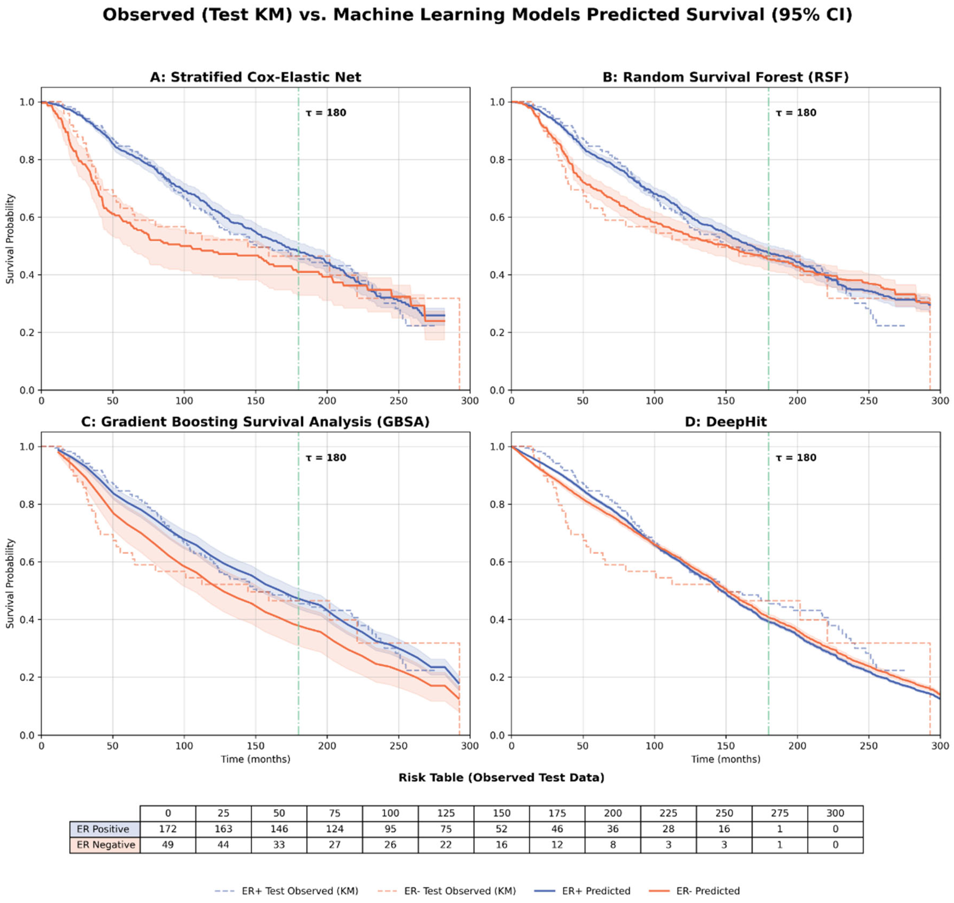
Beyond absolute RMST differences, the qualitative patterns of the predicted survival curves revealed structural differences between architectures (Figure 9). The stratified Cox and RSF models successfully reproduced the empirically observed “crossing” pattern between ER-positive and ER-negative survival curves, reflecting the documented violation of the proportional hazard assumption. In contrast, GBSA generated smoother trajectories without distinct late crossing behavior, likely reflecting the boosting framework’s emphasis on stable global risk ordering, which may dampen late-time fluctuations. DeepHit captured early-stage survival variation but produced more compressed subgroup separation during extended follow-up.

Figure 9. Observed vs. model-predicted survival curves by er status across modeling approaches (test set). Note. Solid lines represent mean predicted survival probabilities with 95% confidence intervals, and dashed lines denote observed Kaplan–Meier survival estimates. Panels display results for (A) Stratified Cox–Elastic Net, (B) Random Survival Forest, (C) Gradient Boosting Survival Analysis, and (D) DeepHit. The risk table below the panels shows the number of patients at risk in the independent test cohort at 25-month intervals (0–300 months) for observed value.

These findings illustrate that similar ranking performance does not ensure faithful representation of time-dependent survival dynamics, underscoring the value of RMST as a complementary framework for clinically meaningful survival interpretation when proportional hazards assumptions are violated.

4. Discussion

In this study, we demonstrated the value of integrating machine learning (ML) with Restricted Mean Survival Time (RMST) to address limitations of traditional survival analysis under non-proportional hazards (PH). Using estrogen receptor (ER) status in the METABRIC cohort as a case study, PH violation was confirmed through Schoenfeld residual diagnostics and crossing Kaplan–Meier curves, highlighting the limitations of hazard ratio-based interpretation in long-term breast cancer survival analysis.

Across Cox elastic net (Cox-ENet), Random Survival Forest (RSF), Gradient Boosting Survival Analysis (GBSA), and DeepHit, discriminative performance on the held-out test set was broadly comparable (C-index ranges 0.66–0.73). However, our results show that discrimination alone is not sufficient for evaluating clinical utility under non-proportional hazards. Despite similar ranking accuracy, the models produced meaningfully different survival curve shapes and absolute survival estimates, particularly for the ER-negative subgroup. Cox E-Net and RSF reproduced the empirically observed crossing pattern, whereas GBSA generated non-crossing trajectories and DeepHit produced more compressed subgroup separation over time. These differences likely reflect underlying model architectures: tree-based methods such as RSF provide flexibility to capture time-varying effects, while boosting frameworks prioritize stable global risk ordering, potentially attenuating late-time divergence.

From a clinical perspective, RSF and GBSA most closely approximated the empirical RMST difference of 16.6 months over 180 months, suggesting balanced estimation of subgroup survival separation. In contrast, Cox-ENet amplified the survival gap, likely due to underestimation of ER-negative survival within a semi-parametric structure that assumes common covariate effects within strata. DeepHit yielded the smallest RMST difference despite competitive discrimination, reflecting its optimization for global risk prediction rather than preservation of clinically defined subgroup separation.

Collectively, these findings highlight a central methodological insight for oncological research: models with statistically similar C-index values can generate substantially different survival structures and absolute time estimates. RMST provides a clinically interpretable, time-based framework that complements discrimination by translating abstract risk scores into meaningful survival duration estimates.

Given that all models were trained and evaluated on the same dataset, formal hypothesis testing between algorithms was not the focus of this work. Rather, our aim was to illustrate how RMST-based evaluation can reveal clinically meaningful differences that are not captured by discrimination metrics alone.

Overall, our results support a shift from retrospective aggregate, population-level summaries toward individualized prognostic survival estimation based on out-of-sample data. By integrating PH diagnostics with ML-based RMST evaluation, survival modeling in oncology can achieve both statistical rigor and enhanced clinical interpretability under non-proportional hazards.

This study has several limitations. First, it is based on a single cohort, the METABRIC dataset, and focuses on ER status as a representative example of non-proportional hazards. As such, the findings may not fully generalize to other disease areas, biomarkers, or settings, and may not fully reflect the complexity of other real-world settings. Future work should evaluate the framework across independent datasets and broader clinical contexts, particularly in settings with diverse biomarkers and varying degrees of non-proportional hazards, to further assess its robustness and generalizability. Despite these limitations, this study presents a principled and clinically interpretable framework for quantifying survival benefit. While conventional metrics such as the C-index and Brier score may vary across datasets, the RMST-centered approach emphasizes time-based clinical interpretation and is designed to be transferable across different disease contexts.

Second, our framework prioritized continuous survival probability estimation and RMST-based interpretation rather than discrete event prediction or traditional “number at risk” tables. Conventional risk tables provide retrospective summaries of observed data density at fixed time points, whereas our objective was to generate out-of-sample predictive survival functions for unseen patients with uncertainty quantified through bootstrap resampling. Future work may integrate survival probability modeling with event-based or multi-state frameworks to jointly characterize individualized trajectories and population-level event dynamics.

Third, RMST estimation depends on the choice of truncation time horizon (τ). While we selected τ = 180 months to reflect long-term breast cancer survival patterns, alternative horizons (e.g., 60 months for 5-year survival) could yield different absolute differences and potentially different agreement patterns across models. Thus, interpretation of RMST differences should consider the clinical context and follow-up duration. Future studies may explore adaptive or multi-horizon RMST evaluation (e.g., τ ∈ {60, 120, 180}) to provide a more complete view of temporal stability and clinical relevance across follow-up windows.

Finally, while the DeepHit model provides a robust framework for survival analysis, our implementation faced challenges in capturing the nuanced survival benefit differences between ER positive and ER Negative cohorts, with predictive significance limited to a one-month horizon. This outcome is likely due to our use of default DeepHit parameters and a generalized survival binning strategy, which was chosen to maintain model generalizability rather than tailoring the architecture to this specific clinical dataset. Furthermore, because deep learning architectures typically require vast datasets and high-dimensional molecular features to achieve peak performance, the current model may not have fully mapped the complex biological interactions of receptor subtypes. Consequently, future research will focus on fine-tuning the survival time bins and integrating higher-dimensional multi-omics data to improve the model’s sensitivity to long-term prognostic variations.

Despite these limitations, the proposed framework effectively integrates machine learning–based survival estimation with the regulator-endorsed RMST approach to address violations of the proportional hazards assumption. We also demonstrated multiple architectures with comparable discrimination and calibration are differed substantially in survival curve structure and RMST-based subgroup estimation. These findings reinforce the importance of combining PH diagnostics, time-dependent evaluation metrics, and RMST-based interpretation when assessing survival models in oncology.

5. Conclusions

The primary objective of this study was to bridge modern machine learning (ML) survival modeling with Restricted Mean Survival Time (RMST), a framework widely recognized in pharmaceutical and regulatory sectors. In oncology datasets like the METABRIC cohort, violations of proportional hazards are frequent, rendering traditional hazard ratio-based approaches less interpretable. While RMST offers a robust alternative, it has traditionally been limited to retrospective, group-level summaries.

In contrast, ML survival models enable individualized survival estimation at the patient level, based on patterns learned from the data. However, their reliance on abstract metrics like the C-index and Brier score often obscures their clinical utility. Our study demonstrated that while Cox Elastic Net, RSF, GBSA, and DeepHit achieved comparable statistical discrimination, they yielded divergent survival trajectories and RMST-based estimates. This underscores a critical finding: comparable statistical accuracy does not necessarily imply similar survival behavior or clinical interpretation, underscoring the need to move beyond single-metric evaluations.

By integrating ML-based survival estimation with RMST quantification, we propose a framework that addresses the proportional hazard violation, unites individualized prognostic power with absolute time units (e.g., months of event-free survival). This approach moves beyond population averages toward personalized survival estimation that maintains regulatory rigor for clinical applications. Ultimately, combining ML with RMST is a symbiotic necessity: RMST provides the transparent meaning that ML lacks, while ML provides the personalization that RMST traditionally misses. Together, they form a coherent strategy for translating complex survival modeling into clear, actionable decision support for personalized oncology.

References

- Singh, R.; Mukhopadhyay, K. Survival analysis in clinical trials: Basics and must know areas. Perspect. Clin. Res. 2011, 2, 145–148. [Google Scholar] [CrossRef] [Scilit] [PubMed]
- Motzer, R.J.; Escudier, B.; Tomczak, P.; Hutson, T.E.; Michaelson, M.D.; Negrier, S.; Oudard, S.; Gore, M.E.; Tarazi, J.; Hariharan, S.; et al. Axitinib versus sorafenib as second-line treatment for advanced renal cell carcinoma: Overall survival analysis and updated results from a randomised phase 3 trial. Lancet Oncol. 2013, 14, 552–562. [Google Scholar] [CrossRef] [Scilit] [PubMed]
- Kurian, A.W.; Sigal, B.M.; Plevritis, S.K. Survival analysis of cancer risk reduction strategies for BRCA1/2 mutation carriers. J. Clin. Oncol. 2010, 28, 222–231. [Google Scholar] [CrossRef] [Scilit] [PubMed]
- Ahmad, T.; Munir, A.; Bhatti, S.H.; Aftab, M.; Raza, M.A. Survival analysis of heart failure patients: A case study. PLoS ONE 2017, 12, e0181001. [Google Scholar] [CrossRef] [Scilit]
- Kelly, P.J.; Lim, L.L.Y. Survival analysis for recurrent event data: An application to childhood infectious diseases. Stat. Med. 2000, 19, 13–33. [Google Scholar] [CrossRef]
- Lin, D.Y.; Wei, L.J. The robust inference for the Cox proportional hazards model. J. Am. Stat. Assoc. 1989, 84, 1074–1078. [Google Scholar] [CrossRef]
- Van Dijk, P.C.; Jager, K.J.; Zwinderman, A.H.; Zoccali, C.; Dekker, F.W. The analysis of survival data in nephrology: Basic concepts and methods of Cox regression. Kidney Int. 2008, 74, 705–709. [Google Scholar] [CrossRef] [Scilit]
- Therneau, T.M.; Grambsch, P.M. Modeling Survival Data: Extending the Cox Model; Springer: New York, NY, USA, 2000. [Google Scholar]
- Bradburn, M.J.; Clark, T.G.; Love, S.B.; Altman, D.G. Survival analysis part II: Multivariate data analysis–an introduction to concepts and methods. Br. J. Cancer 2003, 89, 431–436. [Google Scholar] [CrossRef] [Scilit]
- Kleinbaum, D.G.; Klein, M. Survival Analysis a Self-Learning Text; Springer: Berlin/Heidelberg, Germany, 1996. [Google Scholar]
- Abd ElHafeez, S.; D’Arrigo, G.; Leonardis, D.; Fusaro, M.; Tripepi, G.; Roumeliotis, S. Methods to analyze time-to-event data: The Cox regression analysis. Oxidative Med. Cell. Longev. 2021, 2021, 1302811. [Google Scholar] [CrossRef] [Scilit]
- Collett, D. Modelling Survival Data in Medical Research; Chapman and Hall/CRC: Boca Raton, FL, USA, 2023. [Google Scholar]
- Blagoev, K.B.; Wilkerson, J.; Fojo, T. Hazard ratios in cancer clinical trials—A primer. Nat. Rev. Clin. Oncol. 2012, 9, 178–183. [Google Scholar] [CrossRef] [Scilit]
- Hilsenbeck, S.G.; Ravdin, P.M.; de Moor, C.A.; Chamness, G.C.; Osborne, C.K.; Clark, G.M. Time-dependence of hazard ratios for prognostic factors in primary breast cancer. Breast Cancer Res. Treat. 1998, 52, 227–237. [Google Scholar] [CrossRef] [Scilit] [PubMed]
- Gore, S.M.; Pocock, S.J.; Kerr, G.R. Regression models and non-proportional hazards in the analysis of breast cancer survival. J. R. Stat. Soc. Ser. C (Appl. Stat.) 1984, 33, 176–195. [Google Scholar] [CrossRef] [Scilit]
- Zhu, X.; Zhou, X.; Zhang, Y.; Sun, X.; Liu, H.; Zhang, Y. Reporting and methodological quality of survival analysis in articles published in Chinese oncology journals. Medicine 2017, 96, e9204. [Google Scholar] [CrossRef] [Scilit] [PubMed]
- Cox, D.R. Regression models and life-tables. J. R. Stat. Soc. Ser. B (Methodol.) 1972, 34, 187–220. [Google Scholar] [CrossRef] [Scilit]
- Stel, V.S.; Dekker, F.W.; Tripepi, G.; Zoccali, C.; Jager, K.J. Survival analysis I: The Kaplan-Meier method. Nephron Clin. Pract. 2011, 119, c83–c88. [Google Scholar] [CrossRef] [Scilit]
- In, J.; Lee, D.K. Survival analysis: Part I—Analysis of time-to-event. Korean J. Anesthesiol. 2018, 71, 182–191. [Google Scholar] [CrossRef] [Scilit]
- Rich, J.T.; Neely, J.G.; Paniello, R.C.; Voelker, C.C.; Nussenbaum, B.; Wang, E.W. A practical guide to understanding Kaplan-Meier curves. Otolaryngol.—Head Neck Surg. 2010, 143, 331–336. [Google Scholar] [CrossRef] [Scilit]
- Therneau, T.M. Extending the Cox model. In Proceedings of the First Seattle Symposium in Biostatistics: Survival Analysis; Springer: New York, NY, USA, 1997; pp. 51–84. [Google Scholar]
- Schoenfeld, D.A. Sample-size formula for the proportional-hazards regression model. Biometrics 1983, 39, 499–503. [Google Scholar] [CrossRef] [Scilit]
- Fisher, L.D.; Lin, D.Y. Time-dependent covariates in the Cox proportional-hazards regression model. Annu. Rev. Public Health 1999, 20, 145–157. [Google Scholar] [CrossRef] [Scilit]
- Durrleman, S.; Simon, R. Flexible regression models with cubic splines. Stat. Med. 1989, 8, 551–561. [Google Scholar] [CrossRef] [Scilit]
- Gelman, A.; Hill, J. Data Analysis Using Regression and Multilevel/Hierarchical Models; Cambridge University Press: Cambridge, UK, 2007. [Google Scholar]
- Royston, P.; Parmar, M.K. Restricted mean survival time: An alternative to the hazard ratio for the design and analysis of randomized trials with a time-to-event outcome. BMC Med. Res. Methodol. 2013, 13, 152. [Google Scholar] [CrossRef] [Scilit] [PubMed]
- Hua, K. Design and Analysis of Clinical Trials with Restricted Mean Survival Time. Doctoral Dissertation, Duke University, Durham, NC, USA, 2024. [Google Scholar]
- US Food and Drug Administration. Acute Myeloid Leukemia: Developing Drugs and Biological Products for Treatment-Guidance for Industry. Guidance for Industry. Final; US Food and Drug Administration: Silver Spring, MD, USA, 2022.
- Zhao, L.; Claggett, B.; Tian, L.; Uno, H.; Pfeffer, M.A.; Solomon, S.D.; Trippa, L.; Wei, L.J. On the restricted mean survival time curve in survival analysis. Biometrics 2016, 72, 215–221. [Google Scholar] [CrossRef] [Scilit] [PubMed]
- Calkins, K.L.; Canan, C.E.; Moore, R.D.; Lesko, C.R.; Lau, B. An application of restricted mean survival time in a competing risks setting: Comparing time to ART initiation by injection drug use. BMC Med. Res. Methodol. 2018, 18, 27. [Google Scholar] [CrossRef] [Scilit] [PubMed]
- Kim, D.H.; Uno, H.; Wei, L.J. Restricted mean survival time as a measure to interpret clinical trial results. JAMA Cardiol. 2017, 2, 1179–1180. [Google Scholar] [CrossRef] [Scilit]
- Han, K.; Jung, I. Restricted mean survival time for survival analysis: A quick guide for clinical researchers. Korean J. Radiol. 2022, 23, 495. [Google Scholar] [CrossRef] [Scilit]
- Huang, B.; Kuan, P.F. Comparison of the restricted mean survival time with the hazard ratio in superiority trials with a time-to-event end point. Pharm. Stat. 2018, 17, 202–213. [Google Scholar] [CrossRef] [Scilit]
- Andersen, P.K.; Hansen, M.G.; Klein, J.P. Regression analysis of restricted mean survival time based on pseudo-observations. Lifetime Data Anal. 2004, 10, 335–350. [Google Scholar] [CrossRef] [Scilit]
- Friedman, J.H. Greedy function approximation: A gradient boosting machine. Ann. Stat. 2001, 29, 1189–1232. [Google Scholar] [CrossRef] [Scilit]
- Imani, F.; Chen, R.; Tucker, C.; Yang, H. Random forest modeling for survival analysis of cancer recurrences. In Proceedings of the 2019 IEEE 15th International Conference on Automation Science and Engineering (CASE), Vancouver, BC, Canada, 22–26 August 2019; IEEE: New York, NY, USA, 2019; pp. 399–404. [Google Scholar]
- Chen, T.; Guestrin, C. Xgboost: A scalable tree boosting system. In Proceedings of the 22nd ACM SIGKDD International Conference on Knowledge Discovery and Data Mining, San Francisco, CA, USA, 13–17 August 2016; pp. 785–794. [Google Scholar]
- Hothorn, T.; Bühlmann, P.; Dudoit, S.; Molinaro, A.; Van Der Laan, M.J. Survival ensembles. Biostatistics 2006, 7, 355–373. [Google Scholar] [CrossRef] [Scilit]
- Katzman, J.L.; Shaham, U.; Cloninger, A.; Bates, J.; Jiang, T.; Kluger, Y. DeepSurv: Personalized treatment recommender system using a Cox proportional hazards deep neural network. BMC Med. Res. Methodol. 2018, 18, 24. [Google Scholar] [CrossRef] [Scilit]
- Lee, C.; Zame, W.; Yoon, J.; Van Der Schaar, M. Deephit: A deep learning approach to survival analysis with competing risks. In Proceedings of the AAAI Conference on Artificial Intelligence, New Orleans, LA, USA, 2–7 February 2018; Volume 32. [Google Scholar]
- Pencina, M.J.; D’agostino, R.B. Overall C as a measure of discrimination in survival analysis: Model specific population value and confidence interval estimation. Stat. Med. 2004, 23, 2109–2123. [Google Scholar] [CrossRef] [Scilit] [PubMed]
- Redelmeier, D.A.; Bloch, D.A.; Hickam, D.H. Assessing predictive accuracy: How to compare Brier scores. J. Clin. Epidemiol. 1991, 44, 1141–1146. [Google Scholar] [CrossRef] [Scilit] [PubMed]
- Ridgeway, G. Generalized Boosted Models: A Guide to the gbm Package; R Package Vignette: 2007; Volume 1. Available online: https://CRAN.R-project.org/package=gbm (accessed on 1 January 2026).
- Schenk, A.; Basten, V.; Schmid, M. Modeling the Restricted Mean Survival Time Using Pseudo-Value Random Forests. Stat. Med. 2025, 44, e70031. [Google Scholar] [CrossRef] [Scilit] [PubMed]
- Wang, P.; Li, Y.; Reddy, C.K. Machine learning for survival analysis: A survey. ACM Comput. Surv. (CSUR) 2019, 51, 1–36. [Google Scholar] [CrossRef] [Scilit]
- Wiegrebe, S.; Kopper, P.; Sonabend, R.; Bischl, B.; Bender, A. Deep learning for survival analysis: A review. Artif. Intell. Rev. 2024, 57, 65. [Google Scholar] [CrossRef] [Scilit]
- Zhao, L. Deep neural networks for predicting restricted mean survival times. Bioinformatics 2020, 36, 5672–5677. [Google Scholar] [CrossRef] [Scilit]
- Anderson, W.F.; Chatterjee, N.; Ershler, W.B.; Brawley, O.W. Estrogen receptor breast cancer phenotypes in the Surveillance, Epidemiology, and End Results database. Breast Cancer Res. Treat. 2002, 76, 27–36. [Google Scholar] [CrossRef] [Scilit]
- Duffy, M.J. Estrogen receptors: Role in breast cancer. Crit. Rev. Clin. Lab. Sci. 2006, 43, 325–347. [Google Scholar] [CrossRef] [Scilit]
- Sommer, S.; Fuqua, S.A. Estrogen receptor and breast cancer. In Seminars in Cancer Biology; Academic Press: San Diego, CA, USA, 2001; Volume 11, pp. 339–352. [Google Scholar]
- Bilal, E.; Dutkowski, J.; Guinney, J.; Jang, I.S.; Logsdon, B.A.; Pandey, G.; Sauerwine, B.A.; Shimoni, Y.; Moen Vollan, H.K.; Mecham, B.H.; et al. Improving breast cancer survival analysis through competition-based multidimensional modeling. PLoS Comput. Biol. 2013, 9, e1003047. [Google Scholar] [CrossRef] [Scilit]
- Curtis, C.; Shah, S.P.; Chin, S.F.; Turashvili, G.; Rueda, O.M.; Dunning, M.J.; Speed, D.; Lynch, A.G.; Samarajiwa, S.; Yuan, Y.; et al. The genomic and transcriptomic architecture of 2,000 breast tumours reveals novel subgroups. Nature 2012, 486, 346–352. [Google Scholar] [CrossRef] [Scilit]
- Mayor, S. Chemotherapy and hormonal treatments improve the 15 year survival rate for breast cancer. BMJ Br. Med. J. 2005, 330, 1167. [Google Scholar] [CrossRef] [Scilit]
- Zou, H.; Hastie, T. Regularization and variable selection via the elastic net. J. R. Stat. Soc. Ser. B Stat. Methodol. 2005, 67, 301–320. [Google Scholar] [CrossRef] [Scilit]
- Simon, N.; Friedman, J.H.; Hastie, T.; Tibshirani, R. Regularization paths for Cox’s proportional hazards model via coordinate descent. J. Stat. Softw. 2011, 39, 1–13. [Google Scholar] [CrossRef] [Scilit] [PubMed]
- Pölsterl, S. scikit-survival: A Library for Time-to-Event Analysis Built on Top of scikit-learn. J. Mach. Learn. Res. 2020, 21, 1–6. [Google Scholar]
- Pedregosa, F.; Varoquaux, G.; Gramfort, A.; Michel, V.; Thirion, B.; Grisel, O.; Blondel, M.; Prettenhofer, P.; Weiss, R.; Dubourg, V.; et al. Scikit-learn: Machine learning in Python. J. Mach. Learn. Res. 2011, 12, 2825–2830. [Google Scholar]
- Davidson-Pilon, C. lifelines: Survival analysis in Python. J. Open Source Softw. 2019, 4, 1317. [Google Scholar] [CrossRef] [Scilit]
- Moncada-Torres, A.; van Maaren, M.C.; Hendriks, M.P.; Siesling, S.; Geleijnse, G. Explainable machine learning can outperform Cox regression predictions and provide insights in breast cancer survival. Sci. Rep. 2021, 11, 6968. [Google Scholar] [CrossRef] [Scilit]
- Chen, Y.; Jia, Z.; Mercola, D.; Xie, X. A gradient boosting algorithm for survival analysis via direct optimization of concordance index. Comput. Math. Methods Med. 2013, 2013, 873595. [Google Scholar] [CrossRef] [Scilit]
- Wissel, D.; Janakarajan, N.; Grover, A.; Toniato, E.; Martínez, M.R.; Boeva, V. SurvBoard: Standardized benchmarking for multi-omics cancer survival models. Brief. Bioinform. 2025, 26, bbaf521. [Google Scholar] [CrossRef] [Scilit]
Disclaimer/Publisher’s Note: The statements, opinions and data contained in all publications are solely those of the individual author(s) and contributor(s) and not of MDPI and/or the editor(s). MDPI and/or the editor(s) disclaim responsibility for any injury to people or property resulting from any ideas, methods, instructions or products referred to in the content. |
© 2026 by the authors. Licensee MDPI, Basel, Switzerland. This article is an open access article distributed under the terms and conditions of the Creative Commons Attribution (CC BY) license.