


Abstract
Background: Logistics layouts are commonly evaluated using flow-distance criteria, but layouts with similar economic performance may differ in spatial coverage and pairwise-distance variability. This study examines whether measures of these concepts exhibit distinguishable sensitivity to layout-generation conditions and whether their empirical association supports treating them as complementary rather than redundant descriptors. Methods: Fuzzy LP-Alinks generated layout configurations in a full-factorial simulation comprising 108 conditions and 30 replications per condition; the minimum-flow-distance solution was retained from each run. Coverage was measured with the Normalized Coverage Score (NCS), and distance regularity with the Distance Variability Index (DVI), defined as the coefficient of variation of pairwise distances. Five-factor ANOVAs examined main and interaction effects of object count, link density, virtual-force magnitude, and fuzzy membership function settings, while joint-distribution analyses assessed the association between NCS and DVI. Results: The indicators exhibited different main-effect and interaction patterns. In particular, object count and link density had strong main effects on DVI but nonsignificant main effects on NCS, although their interaction substantially affected NCS. The joint distributions further showed that similar NCS values could coexist with different DVI values. Conclusions: Within the tested experimental setting, the results provide evidence that NCS and DVI behave as complementary rather than directly redundant descriptors of spatial configuration. This conclusion does not imply complete separability or formal discriminant validity.
1. Introduction
A manufacturing layout is usually judged by what it enables to move: parts, people, tools, information, or handling equipment. This operational perspective makes flow-weighted distance indispensable, but it leaves a separate question unresolved: what spatial form does an economically acceptable solution take? Two layouts can impose similar transport effort and nevertheless differ markedly in concentration, unused floor area, and regularity of spacing. These differences matter during early design because they affect which alternatives remain feasible once aisles, buffers, maintenance zones, and future changes are introduced.
The same design problem occurs at several spatial scales. At the micro level, layout decisions concern controls, tools, and materials within a workstation; at the meso level, they concern workstations, cells, and local buffers; and at the macro level, they concern departments, storage zones, transport corridors, and interfaces with automated guided vehicle (AGV) or autonomous mobile robot systems. Across these levels, the meaning of distance changes, but spatial differentiation of solutions with similar economic costs remains relevant.
This paper treats spatial uniformity as a measurement problem rather than as a synonym for a visually dispersed layout. We hypothesize that uniformity has at least two non-equivalent meanings. The first is territorial coverage measured by Normalized Coverage Score (NCS) [1]: whether the object set occupies the external design domain or only a restricted part of it. The second, proposed in this paper Distance Variability Index (DVI), concerns the internal relative regularity of pairwise spatial distances: whether object separations are similar or highly heterogeneous.
Therefore, the primary objective of the study is to determine whether NCS and DVI provide empirically distinguishable and complementary information about spatial configurations within the examined layout-generation setting. The theoretical basis for this comparison lies in their different reference types: NCS evaluates occupation relative to an external spatial domain and reflects its coverage, whereas DVI describes internal heterogeneity in the distribution of pairwise distances. A layout may consequently exhibit high or low coverage with regular spacing, or limited coverage with either regular or heterogeneous internal spacing.
To pursue this objective, the study addresses two interrelated research questions:
RQ1: Factor sensitivity and response structure. How do problem characteristics and heuristic parameters, including their interactions, affect NCS and DVI, and to what extent do the two indicators exhibit distinguishable response patterns?
RQ2: Association and complementarity. What is the empirical association between NCS and DVI across the experimental conditions, and to what extent do their joint distributions indicate that the measures provide complementary rather than redundant information about spatial configurations?
To operationalize these research questions, three evaluation criteria for interpreting the results were specified. Criterion C1 is considered supported when the two indicators exhibit materially different response profiles across the experimental factors, assessed in terms of effect magnitude, direction, and statistical significance. Statistical significance is treated as supporting evidence rather than as the sole basis for distinguishing the indicators. Criterion C2 is considered supported if the measures exhibit different patterns of statistically significant interaction effects or if the same factors produce substantively different conditional responses. Differences between significance decisions in separate models are interpreted descriptively and are not treated as formal tests of equality between the corresponding effects. Criterion C3 is considered supported if the joint distributions do not indicate a one-to-one relationship between the indicators and if similar values of one indicator coexist with materially different values of the other across the experimental conditions. These criteria concern empirical differentiation within the tested experimental setting. They do not constitute a formal test of discriminant validity, complete separability, or statistical independence.
The empirical setting is a family of minimal-flow-distance-selected layouts, generated by a fuzzy linguistic-pattern heuristic [2]. The algorithm is used here as a controlled generator of spatial configurations represented as scatter plots, following an approach initiated by Drezner [3,4], and subsequently developed by, e.g., Grobelny [5,6], Anjos & Vannelli [7], or Castillo & Sim [8]. The heuristic parameters varied in this study regulate the balance between attraction among related objects and separation among inappropriate neighbors, thereby producing a useful range of spatial structures for testing measurement behavior.
1.1. Logistics and Production Management Relevance of Spatial Uniformity
The literature supports treating spatial form as an engineering concern, but it does not support the stronger claim that a uniform layout automatically improves every operational outcome. Most relevant studies examine adjacent constructs as opposed to formal uniformity metrics. The evidence is therefore used to motivate measurement and subsequent verification, not to present uniformity as a sufficient condition for good performance. Table 1 summarizes four management dimensions used to interpret spatial uniformity in logistics and production management. The dimensions are discussed in the following subsections.
Table 1.
Logistics and production management interpretation of spatial uniformity.
1.1.1. Space Utilization and Scalability
Facility-layout research consistently regards floor-space requirements, department geometry, material handling, and static versus dynamic planning as interdependent design issues. Drira et al. [9] provide a broad taxonomy of these formulations and show that layout decisions materially affect manufacturing performance; however, their survey does not establish that local density by itself causes unusable peripheral dead zones. Tompkins et al. [10] likewise include space requirements, aisles, storage, expansion, and renovation in an integrated facilities-planning process, but do not prescribe spatial uniformity as a design rule.
The strongest direct basis for the present argument is the work by Grobelny & Michalski [1], who proposed NCS to quantify how completely a solution occupies a reference design domain. Their contribution supports the claim that coverage is information omitted by the conventional flow–distance objective. It does not justify saying that high NCS guarantees continuously usable reserve space: whether an unoccupied area can accommodate a future machine, aisle, or line depends on its shape, connectivity, clearances, and access. NCS should therefore be interpreted as an early indicator of concentration and coverage, followed by geometric feasibility analysis.
Additional spatial-analysis evidence reinforces this interpretation. Zhou & Murray [11] assess configuration efficiency by aligning observed facility locations with an ideal lattice, providing an external precedent for treating spatial regularity as a measurable property. Lu et al. [12] identified a notable coexistence of spatial expansion and agglomeration in logistics service node facilities, indicating that logistics systems may spread geographically while retaining clustered spatial structures.
Together, these studies support the distinction between domain coverage and local or pairwise spacing, while also showing that regularity must be interpreted relative to the functional context and spatial scale.
1.1.2. Flow Stability, Congestion, and Workload
Zhang et al. [13] modelled workflow congestion in manufacturing and warehouse routing and demonstrated that rerouting can significantly reduce congestion-related delay under specific conditions, particularly at medium traffic intensity. Their findings support the relevance of evaluating route overlap and alternative paths. However, they do not establish that spatial uniformity alone reduces traffic conflicts. Accordingly, the NCS and DVI measures presented in this study should be interpreted as spatial screening descriptors that may support the initial design process by identifying spatial configurations in which the subsequent search for alternative routing solutions could be more promising.
In turn, Benjaafar [14] provides an even stronger caution against relying solely on distance. The study shows that a layout optimized by the conventional quadratic-assignment criterion can be infeasible or poor when judged by work-in-process, and that shorter overall travel distances can coexist with higher work-in-process. Consequently, spatial-uniformity indicators may identify configurations that warrant further operational analysis.
A review by Le-Anh & De Koster [15] concerns AGV guide-path design, fleet sizing, scheduling, routing, conflict resolution, and deadlock resolution. These are explicit design and control problems that cannot be inferred directly from spatial uniformity. However, a more spatially distributed configuration may provide a useful starting point for subsequent routing and traffic-control optimization.
Overall, the studies support the use of spatial-uniformity analysis to classify candidate layouts before conducting routing, queueing, and traffic analyses, instead of treating NCS or DVI as substitutes for operational performance measures. In this paper, such an interpretation is presented as a design rationale rather than an empirically established causal effect of spatial uniformity.
1.1.3. Safety and Access
Safety evidence supports physical separation and access constraints. The UK Health and Safety Executive [16] states that pedestrian and vehicle routes should be separated whenever possible. Spatial-uniformity descriptors may help identify configurations that warrant further examination from the perspective of physical separation and access. They should not, however, be interpreted as evidence of compliance with safety requirements.
Adding a directly relevant warehouse perspective, Cantini et al. [17] demonstrate that mapping forklift movement traces reveals zones with elevated collision and near-miss exposure. Their results support treating mapped route concentrations and conflict points as safety outcomes to be assessed rather than assuming that a regular or broadly covered point pattern is inherently safe. Such adjustments can be considered during early design, although their feasibility and safety consequences require explicit geometric and operational assessment.
Uniform element distribution may also constitute a key consideration in ergonomic design. For instance, Lin & Wu [18] demonstrated the benefits of jointly optimizing accessibility and proximity in interface design, showing that an enhanced link analysis method balancing these requirements for control elements reduced total task completion time in a nuclear power plant control interface experiment. In turn, Sargent et al. [19] introduced a dimensionally accurate optimization method for console layout that integrates actual element dimensions with ergonomic considerations. In addressing such issues, uniform element distribution may be regarded as a supplementary dimension of spatial arrangement, including, in particular, ergonomic quality.
1.1.4. Resilience and Adaptability
The literature supports flexible and dynamic layout planning, but the mechanism is not equivalent to uniform dispersion. Benjaafar & Sheikhzadeh [20] define a flexible plant layout as one that maintains low material-handling cost across stochastic demand scenarios. Their main result concerns strategically located duplicate departments and adaptive flow allocation. Scatter plots featuring uniform facility distribution do not in themselves generate alternative transport pathways or spatial buffers, yet they can expand the analytical perspective during early design phases.
Dynamic-layout research provides a parallel argument for adaptability. Pérez-Gosende et al. [21] review dynamic facility layout as a response to changing flows and sustainability requirements. Saffar et al. [22] develop dynamic layouts for scalable reconfigurable manufacturing systems and evaluate flexibility, throughput, resource utilization, and cost. These contributions motivate testing spatial descriptors against change-scenario performance, but do not make either coverage or spacing regularity a direct measure of reconfigurability.
The presented literature supports including NCS and DVI as complementary descriptors because conventional distance-based evaluation omits aspects of spatial morphology. It does not support deterministic statements that uniformity eliminates dead zones, prevents congestion, guarantees safety, or ensures resilience. Those outcomes depend on additional design variables and should be tested with domain-specific performance models.
1.2. Research Gap and Contributions
The present study forms part of the LP-Alinks research program, in which linguistic patterns, fuzzy variables, and virtual-force mechanisms have previously been used to produce and evaluate facility-layout configurations. Earlier work established the underlying framework for layout-generation and assessment [2], whereas subsequent research introduced NCS to quantify the occupation of a spatial reference domain and examine its relationship with the classical flow-distance objective [1]. These studies provide the methodological basis for the present investigation, but they did not examine whether NCS captures information that is empirically distinguishable from that provided by an alternative measure of internal spatial variability.
The scientific gap addressed here is therefore a measurement-related question. It remains unclear whether a measure of external-domain occupation, such as NCS, and a measure of internal distance variability, such as DVI, represent distinct properties of spatial configurations, whether they respond differently to problem characteristics and heuristic parameters, and whether disagreement between them provides complementary spatial information alongside the conventional flow-distance objective. Thus, the primary objective is to investigate the discriminant behavior of the two indicators within the experimental setting rather than their formal statistical independence. The present study addresses this gap by evaluating NCS and DVI within the same full-factorial simulation experiment. The analysis involves two related dimensions of empirical differentiation: differences in factor sensitivity and interaction structure, and the association between the indicators as reflected in their joint distributions. The purpose is not to identify a universally superior indicator, but to determine whether the two measures provide complementary information about spatial configurations.
The main contributions are threefold. First, the study operationalizes pairwise-distance heterogeneity through the dimensionless DVI and evaluates it alongside NCS within a common experimental framework. Second, it examines whether the indicators exhibit distinguishable main-effect and interaction structures in response to problem characteristics and heuristic parameters. Third, it assesses their empirical association and develops a diagnostic interpretation of combined NCS-DVI profiles, while identifying the methodological limitations related to their use.
2. Theoretical Background: Conceptual and Measurement Framework
2.1. Economic Layout Quality and Spatial Form
The conventional facility layout problem objective aggregates pairwise interaction intensity and separation distance. Optimization-based facility-layout models commonly combine this objective with geometric or relative-positioning constraints. For example, Ohmori & Yoshimoto [23] considered relative-position requirements while minimizing material-handling cost expressed in terms of distances and flows. The conventional objective answers an operational question, specifically how much distance is assigned to important relationships, but it does not address a morphological one: how objects occupy the design domain.
Spatial morphology becomes visible only through additional descriptors, a crucial distinction given that identical flow-distance values can stem from geometrically distinct configurations, particularly in continuous or weakly constrained layouts.
Consequently, spatial descriptors should be interpreted as secondary criteria. Uniform spacing is not intrinsically superior, as technological sequences, shared utilities, consolidation points, or hazardous-area separation often justify deliberate clusters and gaps. Rather, a spatial indicator is valuable when it consistently reveals such structural patterns, enabling the designer to discern whether an observed concentration is intentional or merely an artefact of the search procedure.
2.2. Meanings of Spatial Uniformity
Spatial characteristics are relevant across different classes of engineering systems, although their meaning depends on the modelling context. In distributed-parameter control systems, spatial distribution refers to the evolution of a continuous state over a spatial domain and time; for example, Xu et al. [24] modelled the spatiotemporal dynamics of a parabolic PDE cascade system and examined the stabilization of its spatially distributed state. In facility-layout analysis, by contrast, spatial distribution concerns the geometric arrangement of discrete objects within a design domain. The present study adopts the latter interpretation and focuses on two static properties of layout geometry: external-domain coverage and internal pairwise-distance heterogeneity.
Within this context, spatial uniformity is not an unambiguous concept. It may refer either to the extent to which the objects occupy an externally defined spatial domain or to the regularity of the relative positions of objects. These two meanings are related but conceptually distinct. In the present study, they are referred to as spatial coverage and distance regularity, respectively. The two constructs may converge, but agreement between them is not guaranteed. For example, a regular but compact arrangement may exhibit low distance variability while occupying only a limited part of the reference domain. The following subsections provide their detailed description and operationalizations applied in this study.
2.2.1. Spatial Coverage
Spatial coverage concerns the distribution of objects relative to an externally defined spatial frame. Coverage increases when the occupied locations extend across the reference domain and decreases when objects are concentrated within a limited part of that domain. Unlike distance regularity, this construct is frame-dependent because its assessment requires the specification of an external reference area. It indicates the extent to which the reference spatial domain is represented in a given layout. In this study, spatial coverage is operationalized using the NCS.
NCS was first defined by Grobelny & Michalski [1]. For a layout containing N objects, the design domain is divided into reference cells. If Noccupied denotes the number of cells containing at least one object, the NCS is:
Holding the reference grid and number of objects constant, a larger NCS indicates greater spatial coverage and therefore greater coverage uniformity; a smaller NCS indicates stronger concentration.
In the construction of the NCS reference grid, the number of reference cells is determined by the number of objects instead of being selected as an independent parameter. However, the mapping of the grid onto the external design domain remains context-dependent. The resulting grid is the smallest square grid containing at least N cells. This normalization makes the maximum number of potentially occupied cells dependent on problem size and provides a common basis for comparing layouts generated for different numbers of objects. For the two problem sizes investigated in the present experiment (N = 16 and N = 25), the denominator of NCS is exactly equal to N, since both values are perfect squares. Consequently, the theoretical maximum NCS in these cases is 100%, corresponding to a configuration in which each object occupies a different cell. For non-square values of N, is larger than N, and the mathematical upper bound of the ratio is consequently below 100%.
To guarantee comparability with the earlier study, the original NCS grid construction was retained and mapped onto the same 600 × 600-pixel design domain used by the layout-generation procedure. Within each problem-size condition, the domain boundaries, grid origin, grid construction, and cell geometry were held constant across all factor combinations and replications. This procedure ensured internal comparability of NCS values within the experiment, although it does not establish invariance to alternative domain definitions, grid origins, or spatial resolutions.
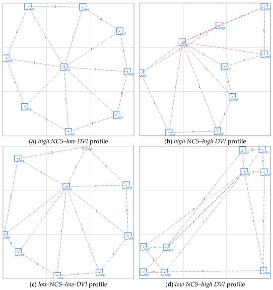
The practical interpretation of NCS is illustrated in Figure 1, where layouts with broad reference-domain coverage exhibit higher NCS values, whereas layouts concentrated within a limited part of the domain exhibit lower values. The figure also demonstrates that a given level of coverage may coexist with different levels of pairwise-distance heterogeneity discussed in the next subsection.
Figure 1.
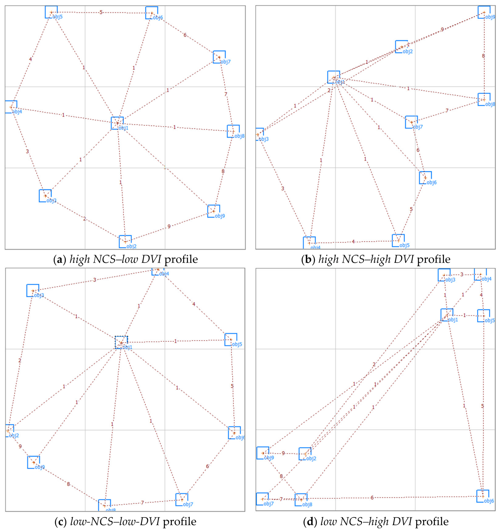
Sample solutions obtained in the illustrative experiment. The result in Panel (a) was obtained using the Convex ML and MD20 settings. NCS = 100% and DVI = 0.347 (high NCS–low DVI). Panel (b) shows the example obtained by LP-Alinks with Linear ML and MD30. NCS = 100% and DVI = 0.400 (high NCS–high DVI). Panel (c) shows an illustrative solution obtained using NmMDS. NCS = 67% and DVI = 0.357 (low-NCS–low-DVI). Panel (d) shows the result obtained for a Concave ML and MD10, where the NCS = 33% and DVI = 0.555 (low NCS–high DVI). Blue squares represent facilities; dashed red lines indicate inter-object relationships, numbers denote relationship values, and light-gray lines represent the reference grid.
2.2.2. Distance Regularity
Distance regularity concerns the variability in the set of pairwise distances between objects. When most pairwise distances are similar, distance variability is low, indicating a relatively regular arrangement of objects. By contrast, when a configuration contains both very short and very long pairwise distances, distance variability is high. This construct is relational and internally referenced because it depends exclusively on the relative positions of the objects. It can therefore be evaluated without considering whether the configuration occupies the entire reference design domain. In this study, distance regularity is operationalized using the DVI, which is defined in the following way.
Let N denote the number of objects in the layout and dij the Euclidean distance between objects i and j. The number of unordered object pairs K is:
the mean pairwise distance:
and DVI is the coefficient of variation of these distances:
where σd denotes the sample standard deviation of pairwise distances.
Although the K pairwise distances constitute the complete finite set of distances for a fixed layout, the sample standard deviation was adopted in this study (with the denominator K − 1). This choice reflects the simulation context, in which each retained layout is treated as one realization of a stochastic layout-generation process and its pairwise distances as an observed realization of the broader distance structure induced by that process. If DVI were used solely as a descriptive measure of one fixed layout, the population standard deviation with denominator K would constitute an equally valid, and arguably more natural, alternative. For N = 16, K = 120, the sample convention exceeds the population value only by a factor of , whereas for N = 25, K = 300, the corresponding factor is merely . Thus, the selected convention has a negligible numerical effect in the present experiment and should be understood as an operational definition rather than the only possible formulation of DVI.
A smaller value of DVI indicates that pairwise distances are more similar and therefore that distance-based uniformity is greater. A larger DVI indicates more heterogeneous spacing and lower distance-based uniformity. This heterogeneity can arise from several geometrically different configurations. For example, it may result from distinct clusters, edge effects, a small number of spatial outliers, or an elongated or anisotropic object arrangement. Therefore, a high DVI should not be interpreted automatically as evidence of any specific geometrical structure. For this purpose, complementary spatial analysis or direct inspection of the configuration is required. Conversely, a low DVI suggests relatively similar pairwise distances but does not by itself establish a particular spatial pattern.
DVI is dimensionless and unchanged by uniform geometric rescaling. This mathematical scale invariance does not imply invariance to problem structure: the number of objects, density of relationships, and attraction pattern can alter the shape of the distance distribution and therefore the index.
2.2.3. Four Profiles of Spatial Uniformity
The joint NCS–DVI space yields four diagnostic profiles. The four NCS–DVI profiles should be regarded as descriptive combinations of domain coverage and distance heterogeneity rather than as definitive classifications of spatial structure. High NCS with high DVI denotes broad coverage combined with heterogeneous pairwise distances. Low NCS with low DVI identifies a relatively compact arrangement with comparatively regular internal spacing, whereas low NCS with high DVI combines restricted domain coverage with heterogeneous spacing. High NCS with low DVI denotes broad and comparatively regular occupation of the design domain. These profiles support interpretation and screening rather than automatic ranking.
Visual representations of the four profiles, obtained using three different parameter sets from the Fuzzy LP-Alinks and one NmMDS solution for an illustrative nine-facility example, are shown in Figure 1. Object relationship values are indicated on the dashed lines. The Fuzzy LP-Alinks algorithm was configured so that agents aimed to maximize the truth values of the two previously characterized patterns. Only the definitions of the fuzzy interpretation of distance and the truth degree of relationship were varied. In subsequent iterations, solutions minimizing the classical flow-distance objective were recorded, and the corresponding NCS and DVI values were saved. The corresponding NCS and DVI values were also calculated for the NmMDS solution. Among the stored sample solutions, those representing the defined profiles were identified. The labels “high” and “low” are used comparatively within the illustrative set and do not represent universal threshold values for NCS or DVI.
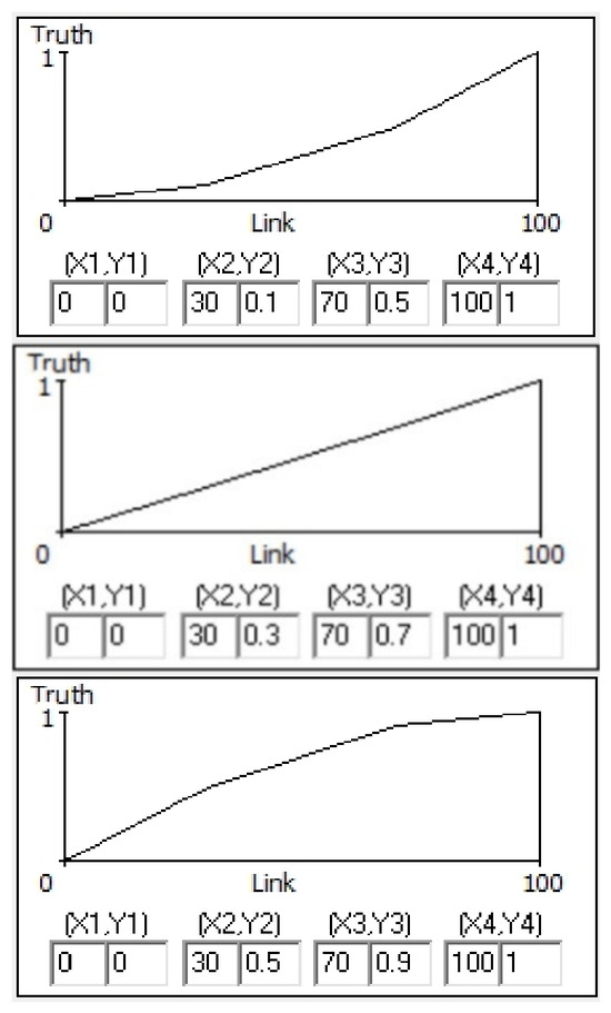
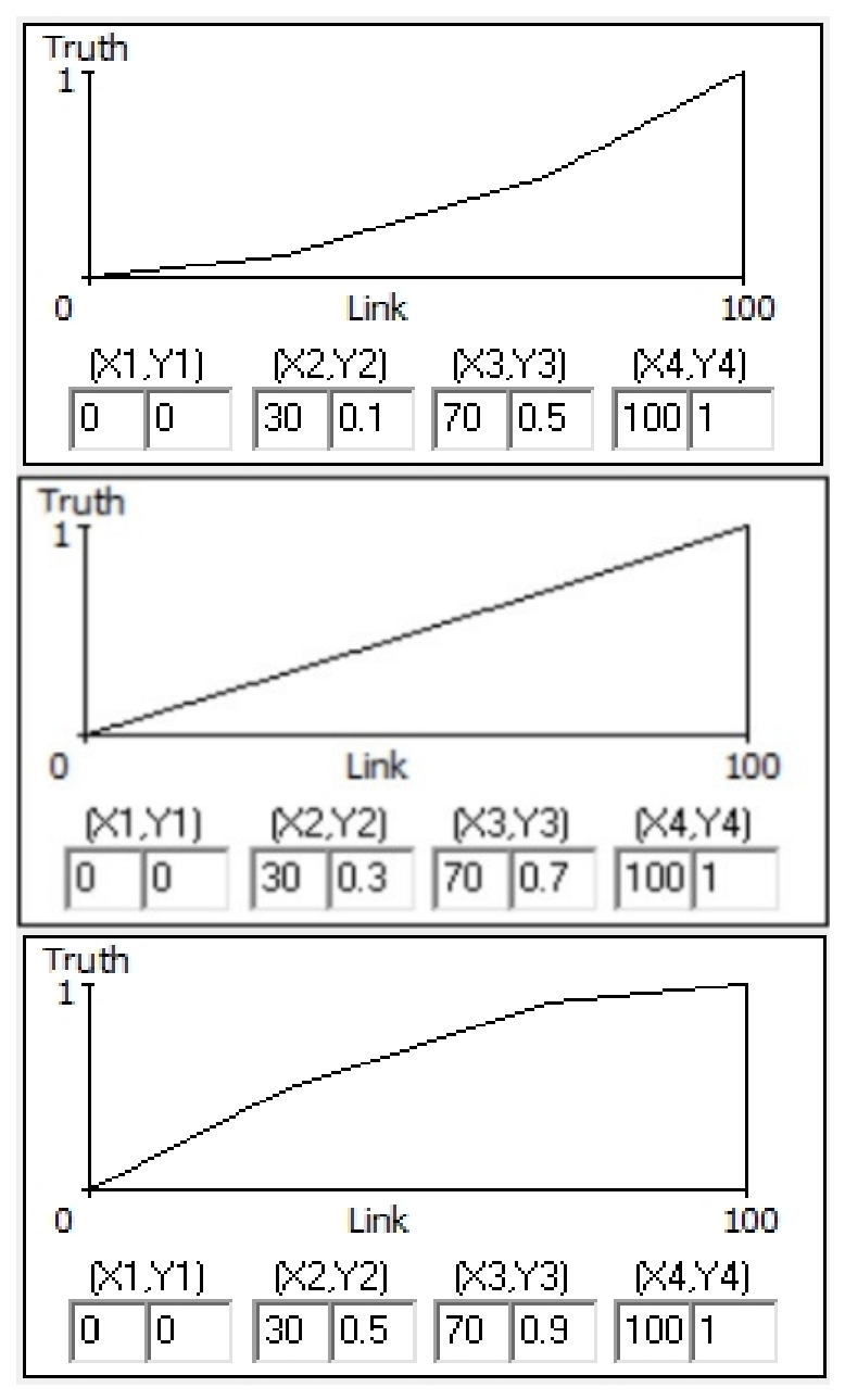
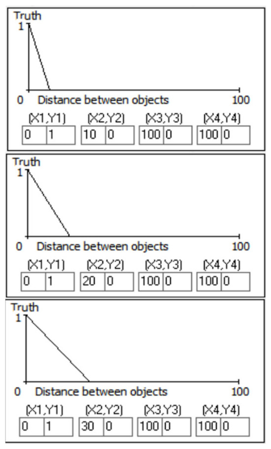
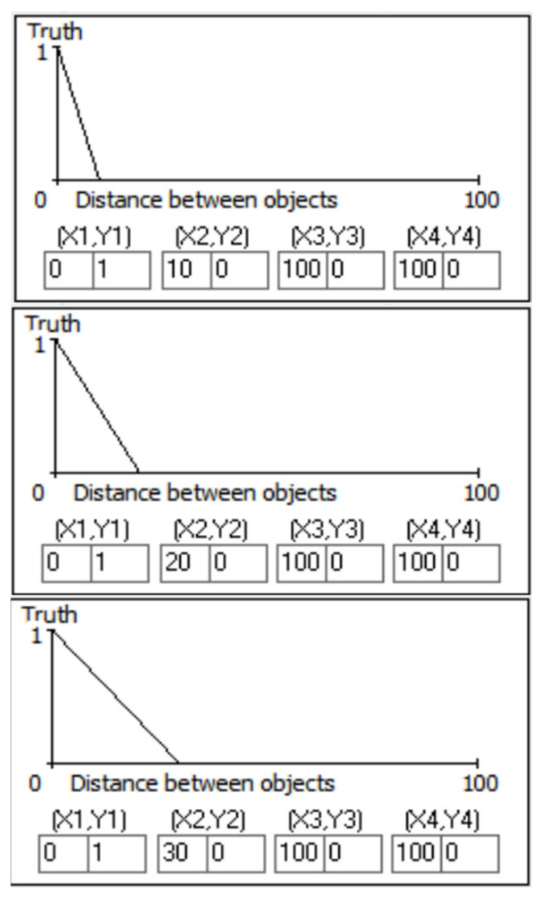
The result in Figure 1a was obtained for Convex ML (see Figure 2) and MD20 level of MD (see Figure 3). The NCS and DVI values are 100% and 0.347, respectively; thus, this layout represents high NCS–low DVI profile. Figure 1b illustrates the result obtained using LP-Alinks with Linear ML and MD30. The values NCS = 100% and DVI = 0.400 allow this solution to be considered representative of the high NCS–high DVI profile. Figure 1c shows the solution obtained using NmMDS. The result, with NCS = 67% and DVI = 0.357, can be considered representative of the low-NCS–low-DVI profile. Figure 1d shows the result obtained using the Concave ML and MD10 settings, where the NCS was 33% and DVI = 0.555. This represents an example of the profile low NCS–high DVI.
Figure 2.
Definition of Concave, Linear and Convex MLs (from top to bottom) for the fuzzy variable Strong relationship; universe of discourse: Percent of the maximum link value between objects.
Figure 3.
Definition of the MD (from top to bottom: MD10, MD20, and MD30) for the fuzzy variable Small Distance; universe of discourse: Percent of the maximum Manhattan distance between objects.
3. Simulation Experiment
3.1. Fuzzy LP-Alinks as an Experimental Generator
LP-Alinks represents design requirements as fuzzy linguistic relationships and converts truth deficits into virtual movements of agents. In the current study, this architecture supplies controlled variation in spatial form. Attraction reflects the requirement that strongly linked objects should be close, whereas the reverse linguistic condition discourages weakly linked objects from remaining close. Virtual-force magnitude and the membership functions assigned to distance and link strength regulate how strongly and over what range these tendencies operate.
In formal terms, the implementation uses Łukasiewicz implication: a → b = min(1, 1 − a + b), and equivalence: a ↔ b = 1 − |a − b|. The forward linguistic condition rewards proximity for strongly related objects, whereas the reverse condition penalizes close placement when the relationship is weak. A truth deficit is converted into a virtual movement, so the force system creates the range of compact, clustered, dispersed, and regular configurations required for comparing DVI with NCS. These definitions are summarized here only to make the experimental factors interpretable; the method itself originates in the earlier LP-Alinks studies.
This paper deliberately avoids reproducing the earlier algorithm-development narrative and uses the heuristic as an experimental instrument for evaluating measurement properties. Only the information necessary to interpret the experiment is repeated here. The rule definitions, movement mechanism, and sustainable-manufacturing demonstrations are reported in [2], while the first definition and economic interpretation of NCS are given in [1].
3.2. Experimental Design
A full five-factor experimental design was used. Table 2 reports the factors, symbols, levels, and their experimental interpretation. Relationship matrices were generated randomly, and nonzero link values were integers from 1 to 9.
Table 2.
Experimental factors and levels.
The full-factorial design combined the levels of NO (2) × LD (2) × VF (3) × MD (3) × ML (3) shown in Table 2. The design comprised 108 conditions. Each condition was replicated 30 times, and every simulation included 100 algorithm iterations corresponding to 100 agent steps. Each simulation yielded a spatial scatter plot of agents/facilities across a 600 × 600 pixel design space. Each scatter plot was additionally scaled up to the full dimensions of the reference design domain.
Across all conditions, 3240 independent simulation runs were performed with 100 algorithm iterations per run, resulting in 324,000 run-level algorithm iterations. For each simulation run, NCS and DVI were recorded for the layout with the minimum classical flow-distance objective value. Thus, the applied procedure imposed objective-conditioned selection on the measurement analysis. Layouts with higher classical flow-distance values but potentially different NCS or DVI characteristics were not retained for the comparison. The reported relationships therefore describe NCS and DVI among economically preferred solutions rather than across the complete population of layouts generated during optimization.
3.3. Dependent Variables and Statistical Analysis
The dependent variables were NCS, for which higher values indicate greater coverage of the reference domain, and DVI, for which lower values indicate greater regularity of pairwise distances. NCS and DVI variables did not participate in the generation or selection of the analyzed layouts.
Separate five-factor full-factorial analyses of variance were performed for NCS and DVI using α = 0.05. Both main effects and interaction effects were examined to address RQ1. The complete ANOVA results are reported in Table A1 and Table A2 of Appendix A.
To address RQ2, the association between NCS and DVI was examined using joint-distribution plots within each NO × LD condition. This analysis was used to determine whether the observations followed a common relationship or whether similar values of one indicator occurred together with different values of the other. The joint-distribution analysis was treated as evidence concerning empirical complementarity rather than as a formal test of statistical independence.
4. Results
4.1. Main Effects of Experimental Factors
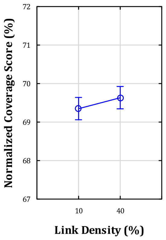
Table 3 reports the five-way full-factorial ANOVA main-effects results discussed in this subsection. For NCS, significant effects were found for VF, ML, and MD. The largest F statistic among the NCS main effects was observed for ML (F = 100), indicating that NCS was particularly sensitive to ML under the tested conditions. Neither NO nor LD significantly differentiated NCS. Although their main effects were nonsignificant, these factors participated in a strong crossover interaction, as demonstrated in Section 4.2. Their marginal effects should therefore not be interpreted independently of their joint levels.
Table 3.
Sensitivity patterns of NCS and DVI: five-factor ANOVA main effects.
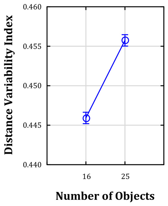
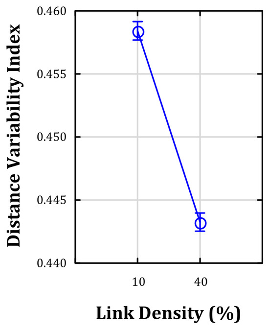
As shown in the DVI columns of Table 3, all investigated factors were significant. The largest F statistic concerned LD (F = 849), followed by NO (F = 356) and the MD (F = 175). The effect of ML was marginal and substantially weaker (F = 3.04, p = 0.048). Thus, the marginal DVI means vary strongly with the structure of the flow problem, whereas the marginal NCS means remain comparatively stable across NO and LD levels. This apparent stability should not be generalized to their joint effect, which is examined in Section 4.2.
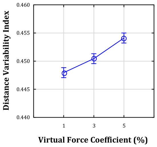
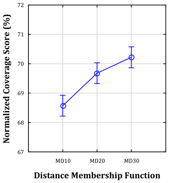
Figure 4, Figure 5, Figure 6, Figure 7, Figure 8, Figure 9, Figure 10, Figure 11, Figure 12 and Figure 13 compare the estimated marginal means of NCS and DVI for the five factors. The figures are arranged in two columns, pairing the measures factor by factor to enable direct comparison of their responses.
Figure 4.
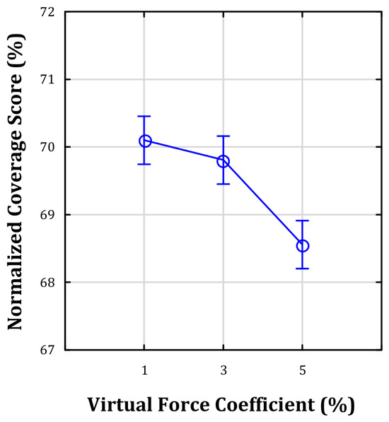
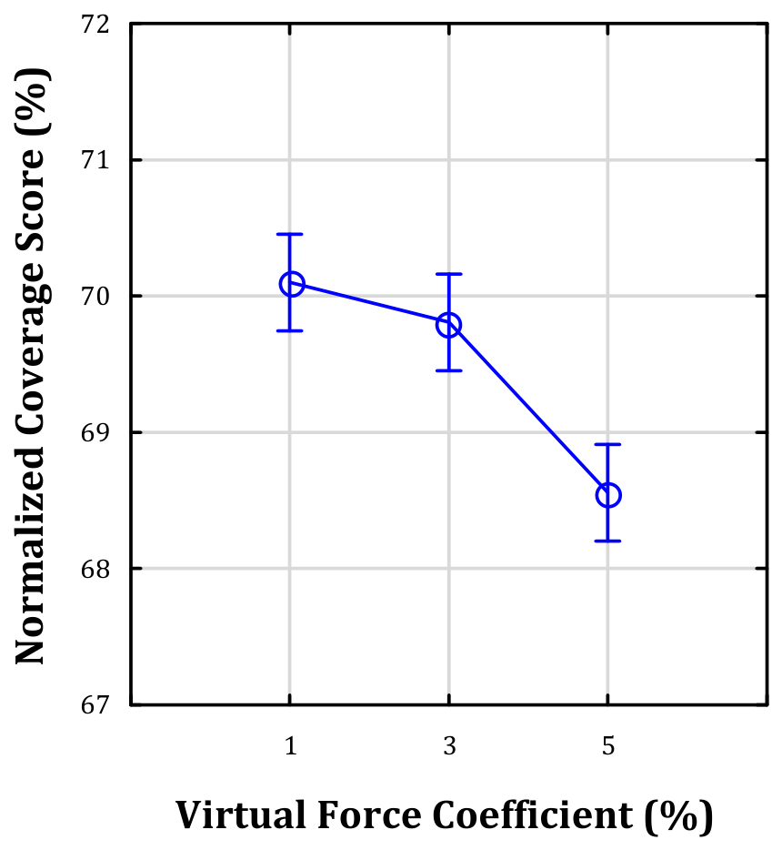
Main effect of VF on NCS. Points represent estimated marginal means. Vertical bars denote 95% confidence intervals. F(2, 3132) = 20.40, p < 0.0001.
Figure 5.
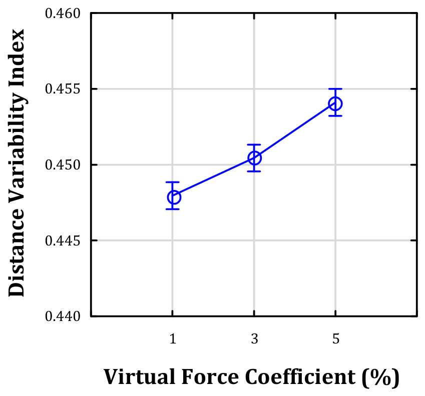
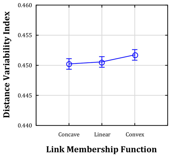
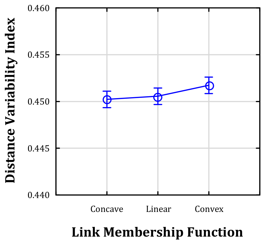
Main effect of VF on DVI. Points represent estimated marginal means. Vertical bars denote 95% confidence intervals. F(2, 3132) = 47.00, p < 0.0001.
Figure 6.
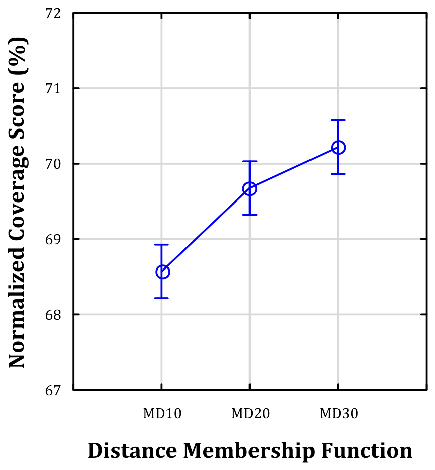
Main effect of MD on NCS. Points represent estimated marginal means. Vertical bars denote 95% confidence intervals. F(2, 3132) = 21.50, p < 0.0001.
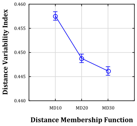
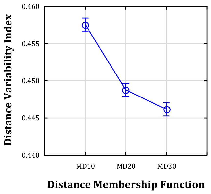
Figure 7.
Main effect of MD on DVI. Points represent estimated marginal means. Vertical bars denote 95% confidence intervals. F(2, 3132) = 175.00, p < 0.0001.
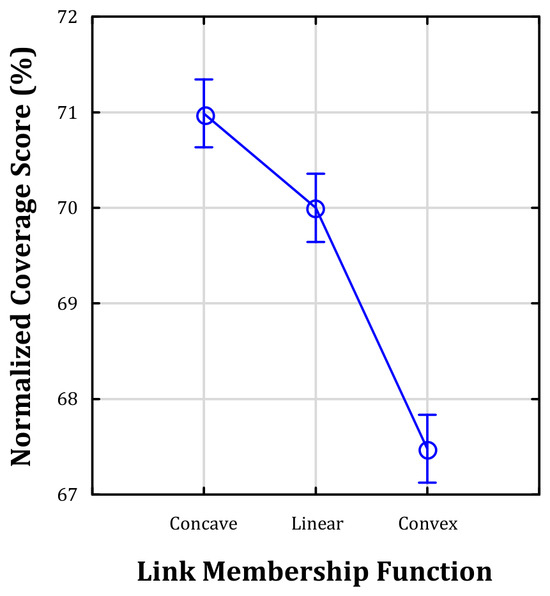
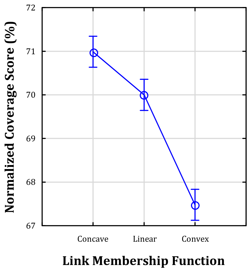
Figure 8.
Main effect of ML on NCS. Points represent estimated marginal means. Vertical bars denote 95% confidence intervals. F(2, 3132) = 99.60, p < 0.0001.
Figure 9.
Main effect of ML on DVI. Points represent estimated marginal means. Vertical bars denote 95% confidence intervals. F(2, 3132) = 3.04, p = 0.0478.
Figure 10.
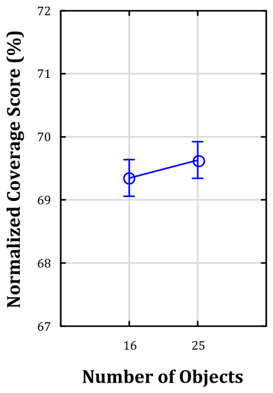
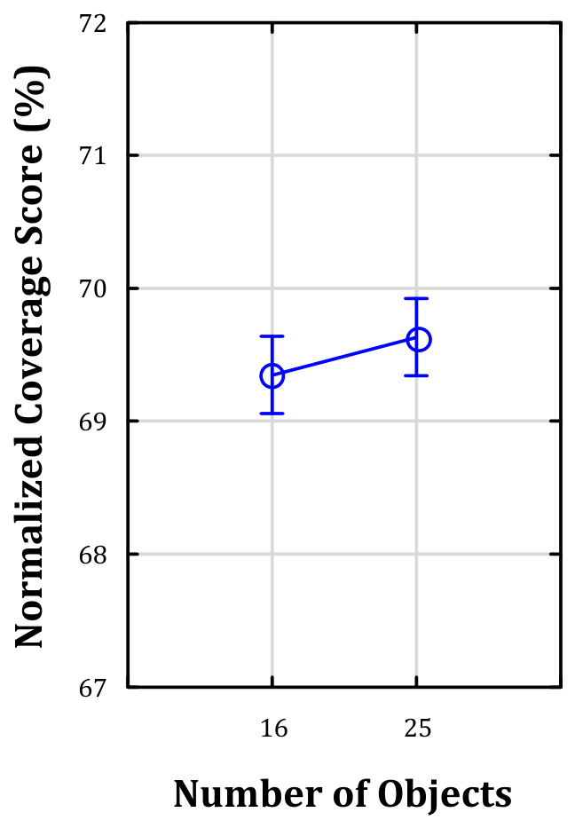
Main effect of NO on NCS. Points represent estimated marginal means. Vertical bars denote 95% confidence intervals. F(1, 3132) = 1.80, p = 0.1746.
Figure 11.
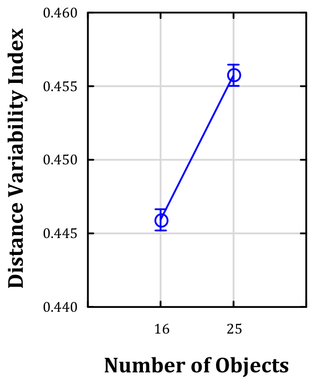
Main effect of NO on DVI. Points represent estimated marginal means. Vertical bars denote 95% confidence intervals. F(1, 3132) = 356.00, p < 0.0001.
Figure 12.
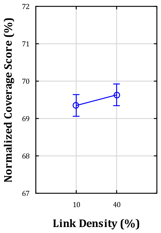
Main effect of LD on NCS. Points represent estimated marginal means. Vertical bars denote 95% confidence intervals. F(1, 3132) = 1.90, p = 0.1737.
Figure 13.
Main effect of LD on DVI. Points represent estimated marginal means. Vertical bars denote 95% confidence intervals. F(1, 3132) = 849.00, p < 0.0001.
Figure 4, Figure 5, Figure 6, Figure 7, Figure 8, Figure 9, Figure 10, Figure 11, Figure 12 and Figure 13 highlight the different sensitivity structures of the measures. Figure 4, Figure 6 and Figure 8 show that NCS changes mainly with VF, MD, and ML, whereas Figure 10 and Figure 12 indicate only small NCS differences for NO and LD. In contrast, Figure 5, Figure 7, Figure 9, Figure 11 and Figure 13 suggest that DVI changes for all five factors, with especially clear differences for NO, LD, and MD. MD30 jointly increases NCS and lowers DVI, whereas increasing VF to 5% lowers NCS and raises DVI. ML primarily differentiates coverage, while NO and LD primarily differentiate distance regularity.
Factor-level Fisher’s LSD post hoc comparisons indicated that VF = 1% and MD30 were associated with lower DVI values in the analyzed conditions. The Convex ML had a slightly unfavorable effect, while the Linear and Concave functions differed little. For NCS, the Concave ML was associated with the highest marginal NCS values, MD30 was also associated with higher marginal coverage, and VF values of 1% and 3% produced higher marginal NCS values than VF = 5%. These comparisons should be interpreted as marginal patterns rather than universally preferable parameter settings because several interaction effects were statistically significant.
With reference to the criteria defined in the introduction, Criterion C1 is supported by the different patterns of main effects summarized in Table 3 and Figure 4, Figure 5, Figure 6, Figure 7, Figure 8, Figure 9, Figure 10, Figure 11, Figure 12 and Figure 13. In particular, NO and LD have strong main effects on DVI but nonsignificant main effects on NCS. In contrast, ML has a pronounced effect on NCS but only a weak, marginally significant effect on DVI. VF and MD affect both indicators, although the magnitude of their effects differs. Thus, the evidence for C1 concerns the overall configuration of factor sensitivities, not the complete separation of the two indicators.
4.2. Interaction Effects of Experimental Factors
The main effects described above summarize marginal differences across factor levels, but the full factorial analysis also reveals substantial interaction effects. These interactions are important because a weak or nonsignificant main effect does not imply that a factor is irrelevant under all combinations of the remaining experimental conditions.
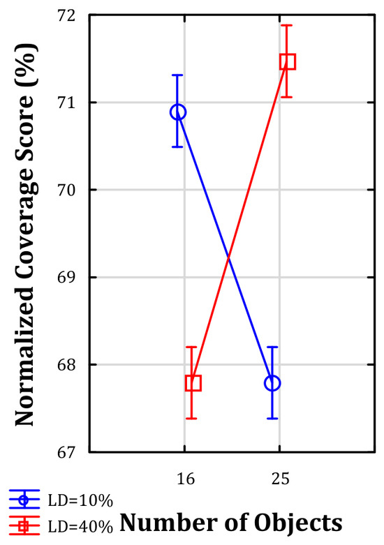
For NCS, the strongest interaction is NO × LD (F(1, 3132) = 263.10, p < 0.0001). The interaction between NO and ML is also significant, F(2, 3132) = 17.60, p < 0.0001. Additional significant two-factor interactions for NCS include VF × NO, VF × LD, and LD × ML. Several higher-order interactions involving MD are also statistically significant.
For DVI, the NO × LD interaction is also statistically significant, F(1, 3132) = 76.0, p < 0.0001, accompanied by LD × ML with F(2, 3132) = 37.0, p < 0.0001. Other statistically significant two-factor interactions include VF × LD, NO × ML, VF × MD, NO × MD, LD × MD, and ML × MD. Also here a number of higher-order interactions are statistically significant, indicating that the effect of one factor may depend on combinations of other experimental settings.
The particularly strong NO × LD interaction for NCS qualifies the interpretation of its nonsignificant marginal effects for NO and LD. Thus, the nonsignificant main effects reported in the previous section should not be interpreted as evidence that NO and LD are irrelevant to NCS. Instead, their effects are conditional on the particular combination of their levels.
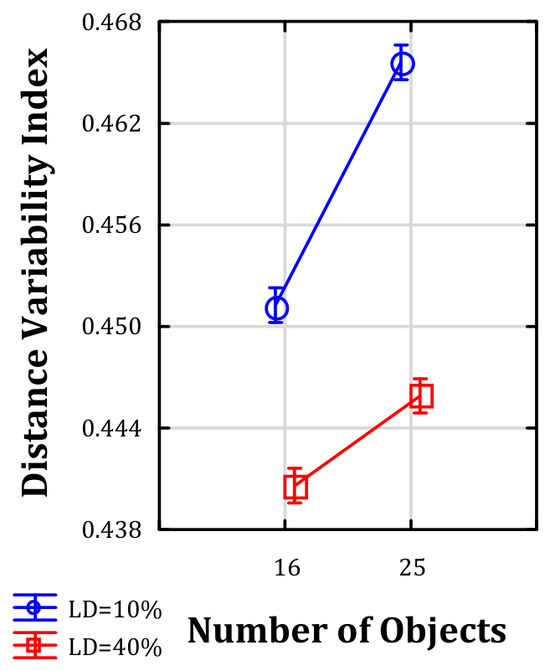
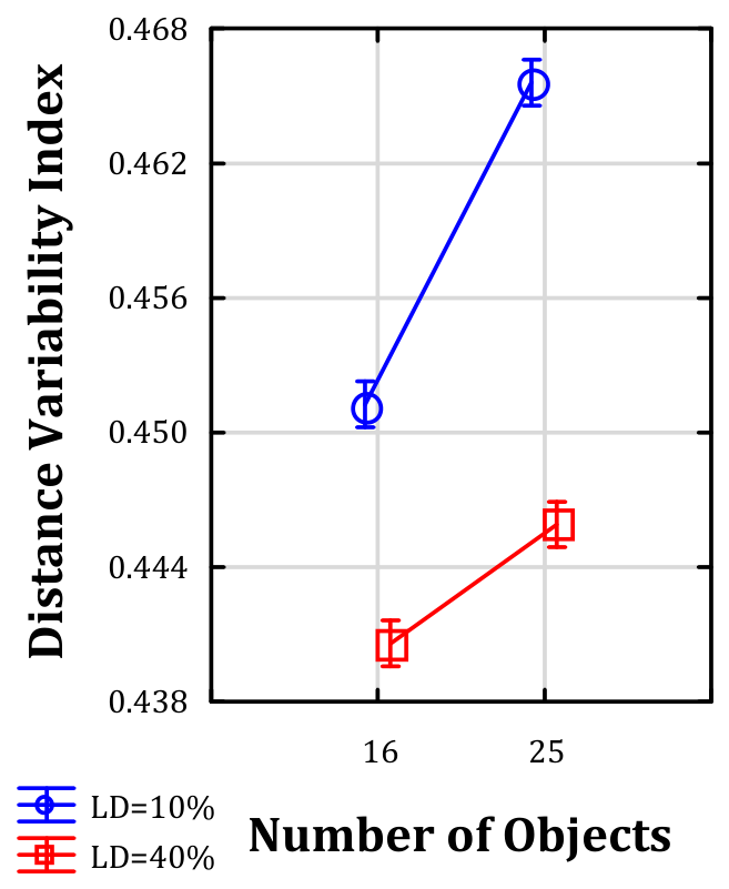
Figure 14 and Figure 15 show that the NO × LD interaction has a different form for NCS and DVI. For NCS, the interaction is crossover in nature. When LD is 10%, increasing NO from 16 to 25 decreases mean NCS, whereas at LD = 40%, the same increase in NO increases mean NCS. These opposing conditional effects largely offset each other when averaged across the levels of the other factor, which explains why the main effects of NO and LD on NCS are nonsignificant despite their strong interaction.
Figure 14.
Interaction between NO and LD for NCS. F(1, 3132) = 263.10, p < 0.0001. Points represent estimated marginal means. Vertical bars denote 95% confidence intervals.
Figure 15.
Interaction between NO and LD for DVI. F(1, 3132) = 76.0, p < 0.0001. Points represent estimated marginal means. Vertical bars denote 95% confidence intervals.
For DVI, the interaction is quantitative rather than crossover. Increasing NO from 16 to 25 increases DVI at both LD levels, indicating greater heterogeneity in pairwise distances. Moreover, DVI is higher at LD = 10% than at LD = 40% for both values of NO. However, the increase in DVI associated with NO is greater at LD = 10%, so the difference between the two LD levels widens as NO increases. Therefore, the NO × LD interaction modifies the magnitude, but not the direction, of the conditional effects on DVI.
Thus, the NO × LD interaction reverses the direction of the conditional effects for NCS, whereas for DVI it changes their magnitude without changing their direction.
The interaction structures are important because they provide additional evidence that NCS and DVI reveal different response structures to changes in the layout-generation conditions. NCS exhibits a particularly strong conditional response to the combination of NO and LD, whereas DVI shows a broader pattern of interactions involving structural and fuzzy-algorithm parameters. At the same time, the presence of numerous significant interactions emphasizes the need to interpret the uniformity indicators in relation to the full factorial structure instead of isolated main effects.
Accordingly, Criterion C2 is supported by differences in the interaction patterns and conditional responses of the two indicators. Although the NO × LD interaction is statistically significant for both measures, its form differs substantially: the conditional NCS effects reverse direction, whereas the conditional DVI effects retain their direction but differ in magnitude. Furthermore, DVI exhibits a broader pattern of significant two-factor interactions than NCS involving LD, VF, ML, MD, and NO. The evidence for C2 therefore concerns the overall configuration, direction, and relative prominence of the interaction effects rather than the exclusive occurrence of an interaction for only one indicator.
4.3. Association and Joint Distribution of NCS and DVI
Section 4.1 and Section 4.2 addressed RQ1 by comparing the main-effect and interaction structures of NCS and DVI. This section addresses RQ2 by examining the association and joint distribution of the two indicators. The purpose is to determine whether their values follow a sufficiently consistent relationship for one measure to serve as a direct proxy for the other or whether the joint observations contain evidence of complementary information.
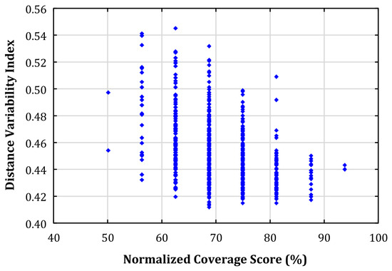
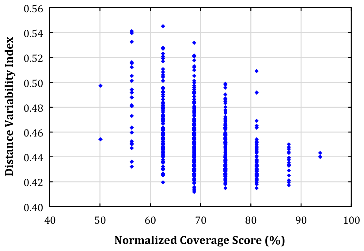
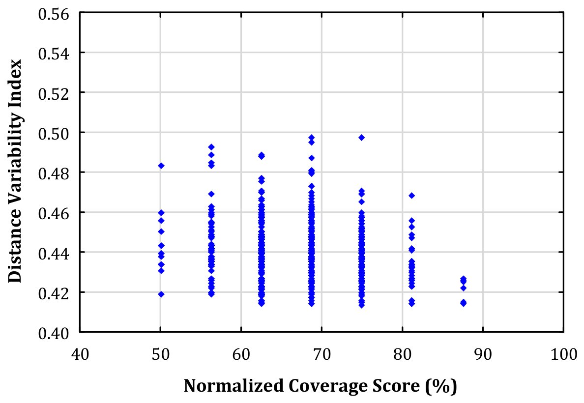
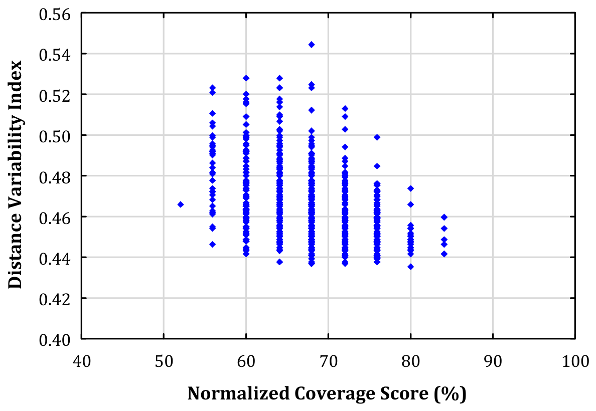
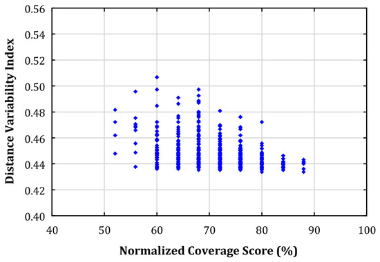
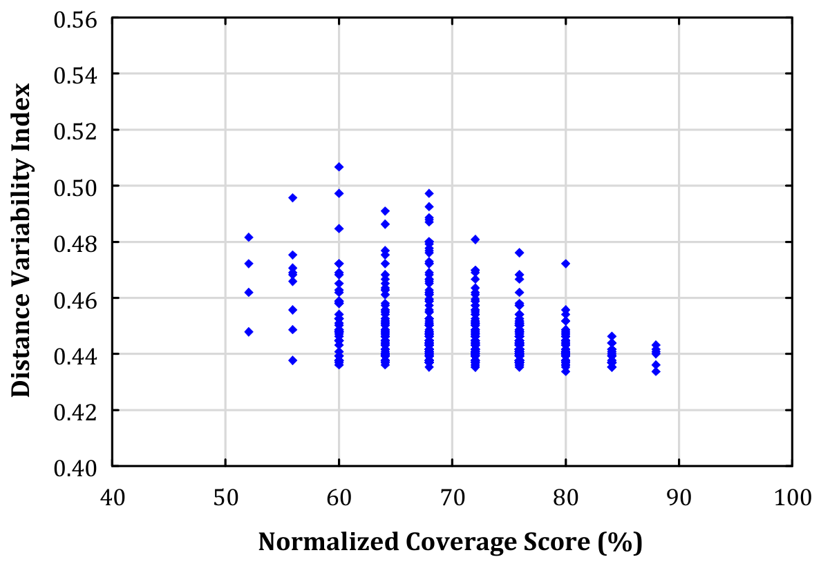
Figure 16, Figure 17, Figure 18 and Figure 19 relate NCS to DVI within each combination of NO and LD. Each point represents the mean NCS and DVI values across 30 replications for one combination of VF, ML, and MD within a given NO × LD condition. The plots provide a direct visual check of whether higher coverage is accompanied by more regular pairwise spacing. Across the four NO × LD conditions, the dominant visual pattern is vertical dispersion: similar NCS values coexist with different DVI values, and the observations do not collapse onto a single deterministic curve. Differences between the NO and LD conditions are more visible along the DVI dimension than as systematic horizontal shifts in NCS.
Figure 16.
Joint NCS vs. DVI distribution for NO = 16 and LD = 10%.
Figure 17.
Joint NCS vs. DVI distribution for NO = 16 and LD = 40%.
Figure 18.
Joint NCS vs. DVI distribution for NO = 25 and LD = 10%.
Figure 19.
Joint NCS vs. DVI distribution for NO = 25 and LD = 40%.
These findings support Criterion C3 by showing that knowledge of NCS alone is insufficient to determine DVI within the analyzed set of experimental condition means. The joint distributions provide evidence that NCS and DVI are not directly interchangeable: NCS describes domain coverage, whereas DVI describes distance heterogeneity. However, this graphical evidence should not be interpreted as demonstrating statistical independence, complete separability, or formal discriminant validity.
5. Discussion
5.1. Addressing the Research Questions
Regarding RQ1, the results provide evidence that NCS and DVI exhibited distinguishable sensitivity to the experimental factors and their interactions. DVI was strongly responsive to NO and LD at the main-effect level, whereas the corresponding NCS main effects were nonsignificant. Additionally, several fuzzy-algorithm parameters produced more pronounced main effects on NCS than on DVI. The interaction plots show that different response patterns for NO and LD do not mean that these factors are irrelevant to NCS. Their effects on NCS reverse direction across the experimental conditions: increasing NO raises NCS when LD is high but lowers NCS when LD is low. For DVI, by contrast, increasing NO raises the indicator at both LD levels, although the magnitude of these effects varies. The different interaction forms strengthen the evidence for C2 because the distinction concerns not only statistical significance but also the directions of the conditional responses. Overall, the different main-effect and interaction structures support C1 and C2 and indicate that the measures respond differently to changes in layout-generation conditions.
In response to RQ2, the joint NCS-DVI distributions show that the indicators provide complementary rather than directly redundant information. Similar NCS values frequently coexist with different DVI values, showing that the extent of domain coverage does not determine the heterogeneity of pairwise distances. Accordingly, the joint-distribution evidence supports Criterion C3 within the tested experimental setting.
Taken together, these findings indicate that NCS and DVI provide empirically distinguishable and complementary information about spatial configurations within the examined layout-generation setting. This conclusion, however, does not imply formal statistical independence or universal discriminant validity and should be interpreted conditionally, within the experimental scope of the study.
5.2. Relationship to Previous Studies
The findings extend two earlier studies. Grobelny & Michalski [2] showed that adding the reverse linguistic rule: “IF objects are close to each other THEN their degree of relationship is high” generates less cluttered and more dispersed scatter plots than using only the unidirectional proximity condition: “IF the degree of relationship is high THEN objects are close to each other”.
The present results explain why that visual difference cannot be represented adequately by a single generic label: dispersion may refer to wider domain occupation, more regular separations, or both. Grobelny & Michalski [1] formalized NCS and investigated the economic–coverage trade-off. The present analysis adds a second measurement axis.
As a result, this study not only complements prior research but also indicates that, within the examined experimental setting, spatial uniformity cannot be adequately characterized using either NCS or DVI alone.
5.3. Applications of NCS and DVI in Logistics and Production Management
NCS and DVI should be used in logistics and production management as complementary screening and interpretation variables, not as substitutes for operational performance measures. NCS identifies global concentration relative to a reference domain, whereas DVI identifies heterogeneity in pairwise spacing. DVI should not, however, be used as an independent clustering detector.
The four NCS-DVI profiles summarize the resulting combinations of external-domain coverage and internal distance heterogeneity. These profiles are descriptive rather than evaluative and should not be interpreted as a ranking of layouts. Moreover, because high DVI may reflect clustering, boundary effects, outliers, or elongated geometry, identifying a specific spatial mechanism requires additional geometric or point-pattern analyses.
Together with the primary flow-distance objective, they help classify candidate layouts and reveal morphology that the economic criterion may omit.
The proposed screening framework applies to the minimal-flow-distance-selected solutions retained in the present experiment and should not be interpreted as representing the full solution population. Their interpretation is conditional. High NCS does not guarantee usable expansion space, which also depends on the size, shape, connectivity, access, clearances, and utilities of the remaining area. Likewise, favorable NCS or DVI values do not demonstrate low congestion, safe traffic, or adaptability. These outcomes depend on routing, capacities, queues, intersections, visibility, separation, relocation options, and change scenarios [13,14,17,20].
Accordingly, a practical evaluation procedure is to screen feasible alternatives using flow-distance cost, NCS, and DVI, and then validate shortlisted layouts with geometric checks, routing or discrete-event simulation, safety assessment, and change-scenario analysis. A comparable separation between layout optimization and operational validation can be found in [25], who combined genetic-algorithm-based layout redesign with workflow simulation to evaluate the resulting operational performance. This type of integrated procedure illustrates how spatial descriptors can be supplemented with independent process-based measures rather than interpreted as direct proxies for operational outcomes. This preserves the diagnostic value of both indicators without attributing causal effects that they were not designed to measure.
5.4. Limitations and Future Research
Several limitations should be considered when interpreting the results. First, although the number of reference cells in NCS is determined by the number of objects, the geometric interpretation of NCS remains dependent on the reference design domain onto which the grid is mapped. The dimensions and boundaries of this domain determine the physical dimensions of the reference cells and may therefore influence whether nearby objects occupy the same cell or different cells.
In the present experiment, the reference-domain definition and grid construction were held constant within each problem-size condition: layouts generated for the same value of N were evaluated using identical domain boundaries, grid origins, and cell geometry. This procedure controlled grid-related variation within the factorial experiment and ensured comparability across experimental treatments. However, this internal control should not be interpreted as evidence that NCS is invariant to alternative domain definitions, grid placements, boundary treatments, or spatial resolutions. A systematic sensitivity analysis of these aspects would constitute a separate methodological investigation and is beyond the scope of the present study. For this reason, NCS should be interpreted as a context-dependent measure of coverage, and comparisons across studies or applications require an explicitly specified reference domain and grid construction.
Next, NCS and DVI were evaluated only for the layout solution that minimized the classical flow-distance objective in each simulation run. The results therefore characterize spatial-uniformity measures among flow-distance-selected, economically preferred solutions rather than across the complete population of layouts generated during optimization. Layouts with higher flow-distance values but potentially different NCS and DVI characteristics were not included in the measurement analysis. The same selection rule was applied consistently across all experimental conditions, so the factorial comparison remains internally consistent; nevertheless, the restriction limits the generalizability of the findings to the broader solution space. Future research could retain NCS and DVI for all generated layouts, or for a pre-specified Pareto-relevant subset, and examine whether the observed sensitivity patterns persist without conditioning the measurement analysis on the minimum classical flow-distance solution.
Third, DVI measures heterogeneity in the distribution of pairwise distances but does not uniquely identify the geometric source of that heterogeneity. A high DVI may result from spatial clustering, isolated outlying objects, boundary effects, elongated or anisotropic configurations, or combinations of these phenomena. Therefore, DVI should not be interpreted as a standalone clustering indicator. Future studies should compare DVI with complementary spatial point-pattern and geometric measures capable of distinguishing these alternative spatial mechanisms.
Moreover, the full-factorial analysis revealed numerous statistically significant interaction effects. These findings indicate that the effect of one experimental factor may depend on the levels of other factors and that marginal main effects do not always provide a complete description of the response structure. The present study discusses the most prominent interactions relevant to the research questions, while the complete ANOVA results are provided in Appendix A. A comprehensive interpretation of all higher-order interactions would require a separate analysis and is therefore identified as a direction for future research. Such research should systematically examine conditional effects, interaction plots, and effect-size measures, including higher-order interactions where substantively justified.
Finally, the study is simulation-based and uses randomly generated relationship structures. It does not account for unequal object shapes and areas, building-specific geometric constraints, time-varying flows, or actual traffic conflicts. Unequal-area facility-layout formulations explicitly incorporate fixed facility shapes, non-overlap requirements, and material-travel objectives, as illustrated by McKendall & Hakobyan [26]. Extending the present measurement framework to such formulations would make it possible to examine how NCS and DVI behave when spatial configurations are constrained by realistic facility dimensions and geometric feasibility requirements. Consequently, the present results establish geometric and measurement behavior rather than direct operational effects. Further validation using real facility-layout data is needed, together with routing, queueing, safety, and change-scenario analyses. Coupling LP-Alinks with discrete-event or agent-based traffic simulation could provide a basis for testing whether different NCS–DVI profiles are associated with differences in travel time, queueing, route conflicts, vehicle utilization, or disturbance-recovery performance.
A natural extension of the present study would be to incorporate NCS and DVI directly into the layout-search procedure. Together with the classical flow-distance criterion, this would define a multi-objective optimization problem involving the minimization of flow-distance and DVI and the maximization of NCS. Both weighted aggregation and Pareto-based approaches could be applied to identify layouts representing different trade-offs among these criteria. The results of such experiments would enable comparison of the resulting layouts with those obtained using the flow-distance objective alone. Other multi-objective extensions integrating flow cost, spatial descriptors, safety, and logistics resilience, as well as adaptations to three-dimensional and multi-level environments such as high-bay warehouses, also represent relevant directions for future research.
6. Conclusions
This study examined spatial uniformity as a multidimensional measurement problem and compared two complementary indicators: NCS, which describes the occupation of an externally defined design domain, and DVI, which describes heterogeneity in the distribution of pairwise spatial distances. The results provide evidence that the two indicators exhibit distinguishable response structures under the experimental conditions considered.
The specified evaluation criteria were supported within the tested experimental setting. Criterion C1 was supported by differences in the main-effect patterns of the indicators, particularly for NO, LD, and ML. Criterion C2 was supported by differences in the interaction structures and conditional responses of the indicators. In particular, the NO × LD interaction was crossover in form for NCS, whereas for DVI it modified the magnitude but not the direction of the conditional effects. Criterion C3 was supported by the joint distributions, in which similar NCS values coexisted with substantially different DVI values. Taken together, these findings address RQ1 and RQ2 and support the interpretation that NCS and DVI exhibit empirically distinguishable and complementary behavior within the tested experimental setting. They do not, however, demonstrate complete separability, statistical independence, or universal discriminant validity.
The four NCS–DVI profiles provide a diagnostic framework for distinguishing configurations characterized by different combinations of external-domain coverage and internal distance heterogeneity. However, these profiles should not be interpreted as a universal ranking of layouts or as direct evidence of operational superiority. Instead, they describe different spatial characteristics that may be relevant depending on the objectives and constraints of a particular layout-design problem.
The findings should be interpreted within the methodological boundaries of the study. First, NCS depends on the definition of the external reference domain and the selected grid resolution. Its absolute value may therefore change when these methodological settings are modified. Second, NCS and DVI were evaluated exclusively for solutions selected according to the classical flow-distance objective. Consequently, the results characterize flow-distance-preferred layouts rather than the complete population of generated configurations. Third, DVI does not uniquely identify the geometric mechanism underlying distance heterogeneity. In particular, a high DVI value should not automatically be interpreted as evidence of clustering because it may also result from boundary effects, isolated objects, asymmetric distributions, or elongated layout geometries. Identifying the underlying structure requires complementary geometric or spatial point-pattern analyses.
In practical applications, the combined use of NCS and DVI can broaden the evaluation of candidate layouts when applied alongside the primary flow-distance criterion, geometric feasibility checks, and independent operational analyses. In particular, these indicators may support the preliminary classification of spatial configurations before detailed evaluations of routing, congestion, safety, and adaptability are conducted. However, neither indicator should be assumed to imply reduced traffic conflicts, improved routing performance, or greater operational resilience without explicit empirical or simulation-based verification.
Overall, joint reporting of NCS and DVI can enhance the assessment of facility-layout configurations by combining information about external-domain coverage and internal distance heterogeneity. For both practical and scientific applications, such reporting should specify the reference domain and grid resolution used to calculate NCS, the procedure applied to select layouts, and the relevant interaction effects. Where operational conclusions are required, NCS and DVI should be supplemented with independent measures of routing efficiency, traffic performance, safety, and adaptability.
Author Contributions
Conceptualization, methodology, software, formal analysis, investigation, resources, data curation, writing—original draft preparation, writing—review and editing, visualization, project administration, R.M. and J.G. All authors have read and agreed to the published version of the manuscript.
Funding
The work was partially financially supported by the Polish National Science Centre grant no. 2019/35/B/HS4/02892: Intelligent approaches for facility layout problems in management, production, and logistics.
Data Availability Statement
The data presented in this study are available upon reasonable request from the corresponding author.
Acknowledgments
During the preparation of this manuscript, the authors used Microsoft Copilot (GPT-5.6) for the purposes of language editing, proofreading, grammatical corrections, paraphrasing, and creating the graphical abstract. The authors have reviewed and edited the output and take full responsibility for the content of this publication. All authors have read and agreed to the published version of the manuscript.
Conflicts of Interest
The authors declare no conflicts of interest.
Abbreviations
The following abbreviations are used in this manuscript:
| AGV | Automated guided vehicle |
| ANOVA | Analysis of variance |
| DVI | Distance Variability Index |
| LD | Relative link density, calculated as the number of nonzero links divided by the maximum possible number of links in a fully connected network. |
| LP | Linguistic Pattern |
| LP-Alinks | Linguistic-pattern-based Alinks algorithm |
| MD | Distance membership function |
| MD10, MD20, MD30 | Levels of the distance membership function |
| ML | Link membership function |
| NCS | Normalized Coverage Score |
| NO | Number of objects in the facility layout problem |
| RQ | Research question |
| VF | Virtual-force magnitude coefficient, expressed as the single-step object displacement for the maximum virtual force relative to the maximum dimension of the design area. |
Appendix A
Table A1.
Full five-way factorial analysis of variance for Normalized Coverage Score.
Table A2.
Full five-way factorial analysis of variance for Distance Variability Index.
References
- Grobelny, J.; Michalski, R. Linguistic-pattern-based optimization of economic and spatial uniformity criteria in facility layout problems. Cent. Eur. J. Oper. Res. 2026, 1–33. [Google Scholar] [CrossRef] [Scilit]
- Grobelny, J.; Michalski, R. Linguistic Pattern-Based Facility Layout Optimization in Designing Sustainable Manufacturing Systems. IEEE Trans. Fuzzy Syst. 2025, 33, 4167–4179. [Google Scholar] [CrossRef] [Scilit]
- Drezner, Z. DISCON: A New Method for the Layout Problem. Oper. Res. 1980, 28, 1375–1384. [Google Scholar] [CrossRef] [Scilit]
- Drezner, Z. A Heuristic Procedure for the Layout of a Large Number of Facilities. Manag. Sci. 1987, 33, 907–915. [Google Scholar] [CrossRef] [Scilit]
- Grobelny, J. The fuzzy approach to facilities layout problems. Fuzzy Sets Syst. 1987, 23, 175–190. [Google Scholar] [CrossRef] [Scilit]
- Grobelny, J. On one possible fuzzy approach to facilities layout problems. Int. J. Prod. Res. 1987, 25, 1123–1141. [Google Scholar]
- Anjos, M.F.; Vannelli, A. An Attractor-Repeller approach to floorplanning. Math. Methods Oper. Res. 2002, 56, 3–27. [Google Scholar] [CrossRef] [Scilit]
- Castillo, I.; Sim, T. A spring-embedding approach for the facility layout problem. J. Oper. Res. Soc. 2004, 55, 73–81. [Google Scholar] [CrossRef] [Scilit]
- Drira, A.; Pierreval, H.; Hajri-Gabouj, S. Facility layout problems: A survey. Annu. Rev. Control 2007, 31, 255–267. [Google Scholar] [CrossRef] [Scilit]
- Tompkins, J.A.; White, J.A.; Bozer, Y.A.; Tanchoco, J.M.A. Facilities Planning, 4th ed.; John Wiley & Sons: Hoboken, NJ, USA, 2010. [Google Scholar]
- Zhou, E.; Murray, A.T. Facility Layout and Spatial Configuration Efficiency Assessment. Netw. Spat. Econ. 2025, 25, 487–511. [Google Scholar] [CrossRef] [Scilit]
- Lu, J.; Luo, J.; Tian, L.; Tian, Y. Spatial Patterns and the Evolution of Logistics Service Node Facilities in Large Cities—A Case from Wuhan. ISPRS Int. J. Geo-Inf. 2024, 13, 82. [Google Scholar] [CrossRef] [Scilit]
- Zhang, M.; Batta, R.; Nagi, R. Modeling of Workflow Congestion and Optimization of Flow Routing in a Manufacturing/Warehouse Facility. Manag. Sci. 2009, 55, 267–280. [Google Scholar] [CrossRef] [Scilit]
- Benjaafar, S. Modeling and Analysis of Congestion in the Design of Facility Layouts. Manag. Sci. 2002, 48, 679–704. [Google Scholar] [CrossRef] [Scilit]
- Le-Anh, T.; De Koster, M.B.M. A review of design and control of automated guided vehicle systems. Eur. J. Oper. Res. 2006, 171, 1–23. [Google Scholar] [CrossRef] [Scilit]
- The UK Health and Safety Executive. (n.d.). Separating Pedestrians and Vehicles—HSE. Available online: https://www.hse.gov.uk/workplacetransport/separating.htm (accessed on 18 August 2026).
- Cantini, A.; De Carlo, F.; Tucci, M. Towards Forklift Safety in a Warehouse: An Approach Based on the Automatic Analysis of Resource Flows. Sustainability 2020, 12, 8949. [Google Scholar] [CrossRef] [Scilit]
- Lin, C.J.; Wu, C. Improved link analysis method for user interface design—Modified link table and optimisation-based algorithm. Behav. Inf. Technol. 2010, 29, 199–216. [Google Scholar] [CrossRef] [Scilit]
- Sargent, T.A.; Kay, M.G.; Sargent, R.G. A Methodology for Optimally Designing Console Panels for Use by a Single Operator. Hum. Factors 1997, 39, 389–409. [Google Scholar] [CrossRef] [Scilit] [PubMed]
- Benjaafar, S.; Sheikhzadeh, M. Design of flexible plant layouts. IIE Trans. 2000, 32, 309–322. [Google Scholar] [CrossRef] [Scilit]
- Pérez-Gosende, P.; Mula, J.; Díaz-Madroñero, M. Overview of Dynamic Facility Layout Planning as a Sustainability Strategy. Sustainability 2020, 12, 8277. [Google Scholar] [CrossRef] [Scilit]
- Saffar, F.; Moghaddam, S.K.; Huang, S. Dynamic layout design for scalable reconfigurable manufacturing systems. Int. J. Prod. Res. 2025, 63, 6530–6552. [Google Scholar] [CrossRef] [Scilit]
- Ohmori, S.; Yoshimoto, K. A Primal-Dual Interior-Point Method for Facility Layout Problem with Relative-Positioning Constraints. Algorithms 2021, 14, 60. [Google Scholar] [CrossRef] [Scilit]
- Xu, W.; Zong, G.; Niu, B.; Wang, H.; Zhao, X. Event-based fuzzy adaptive boundary Taylor decoupling control for parabolic PDE cascade systems: A novel nonlinear filters approach. Fuzzy Sets Syst. 2026, 542, 109945. [Google Scholar] [CrossRef] [Scilit]
- Munavalli, J.R.; Rao, S.V.; Srinivasan, A.; Van Merode, F. Dynamic Layout Design Optimization to Improve Patient Flow in Outpatient Clinics Using Genetic Algorithms. Algorithms 2022, 15, 85. [Google Scholar] [CrossRef] [Scilit]
- McKendall, A.; Hakobyan, A. An Application of an Unequal-Area Facilities Layout Problem with Fixed-Shape Facilities. Algorithms 2021, 14, 306. [Google Scholar] [CrossRef] [Scilit]

Disclaimer/Publisher’s Note: The statements, opinions and data contained in all publications are solely those of the individual author(s) and contributor(s) and not of MDPI and/or the editor(s). MDPI and/or the editor(s) disclaim responsibility for any injury to people or property resulting from any ideas, methods, instructions or products referred to in the content. |
© 2026 by the authors. Licensee MDPI, Basel, Switzerland. This article is an open access article distributed under the terms and conditions of the Creative Commons Attribution (CC BY) license.