Filter Learning-Based Partial Least Squares Regression and Its Application in Infrared Spectral Analysis

Abstract

Partial Least Squares (PLS) regression has been widely used to model the relationship between predictors and responses. However, PLS may be limited in its capacity to handle complex spectral data contaminated with significant noise and interferences. In this paper, we propose a novel filter learning-based PLS (FPLS) model that integrates an adaptive filter into the PLS framework. The FPLS model is designed to maximize the covariance between the filtered spectral data and the response. This modification enables FPLS to dynamically adapt to the characteristics of the data, thereby enhancing its feature extraction and noise suppression capabilities. We have developed an efficient algorithm to solve the FPLS optimization problem and provided theoretical analyses regarding the convergence of the model, the prediction variance, and the relationships among the objective functions of FPLS, PLS, and the filter length. Furthermore, we have derived bounds for the Root Mean Squared Error of Prediction (RMSEP) and the Cosine Similarity (CS) to evaluate model performance. Experimental results using spectral datasets from Corn, Octane, Mango, and Soil Nitrogen show that the FPLS model outperforms PLS, OSCPLS, VCPLS, PoPLS, LoPLS, DOSC, OPLS, MSC, SNV, SGFilter, and Lasso in terms of prediction accuracy. The theoretical analyses align with the experimental results, emphasizing the effectiveness and robustness of the FPLS model in managing complex spectral data.

1. Introduction

In the field of Chemometrics, spectral analysis has been a cornerstone for both qualitative and quantitative assessments of various compounds. Among the various spectroscopic techniques, infrared (IR) spectroscopy stands out due to its non-destructive nature, rapid analysis speed, and its ability to provide detailed chemical information. However, the direct interpretation of IR spectra can be challenging due to the complex overlap of absorption bands and the presence of noise. To address this issue, Partial Least Squares (PLS) regression has been widely adopted for spectral data analysis, aiming to establish a linear relationship between predictors and the response [1]. Despite its popularity, PLS regression may suffer from overfitting and reduced predictive performance when dealing with noisy or highly correlated spectral data. This limitation underscores the need to develop more robust and adaptive models that can enhance the accuracy and reliability of spectral-based predictions. The consequences of inaccurate predictions in fields such as food quality control, environmental monitoring, and pharmaceutical analysis can be significant. Therefore, refining spectral analysis techniques is crucial for advancing the precision and applicability of Chemometrics models.

Filtering techniques have traditionally been employed for preprocessing spectral data, aiming to remove noise while enhancing the signal-to-noise ratio [2,3]. However, the application of these filters is often conducted in an unsupervised manner, meaning that they do not account for the ultimate goal of the analysis, which is to establish accurate predictive models. This disconnect between the filtering process and the subsequent regression analysis can potentially compromise the overall performance of the model. To address this gap, this paper introduces a novel filter-based PLS regression model that bridges the divide between data preprocessing and regression analysis. The proposed model integrates the learning of filter parameters and PLS regression into a unified framework, enabling a more efficient and effective analysis pipeline. By leveraging supervised learning on samples, the model simultaneously optimizes both the filter parameters and the PLS regression model, ensuring that the filtering process is aligned with the ultimate goal of accurate prediction.

Previous research in this area has explored various modifications and extensions of PLS regression to enhance its performance. Techniques such as Orthogonal Signal Correction PLS (OSCPLS), Variance Constrained PLS (VCPLS), Powered PLS (PoPLS), Low-pass Filter PLS (LoPLS), Direct Orthogonal Signal Correction (DOSC), Orthogonal Projection to Latent Structures (OPLS), Multiplicative Scatter Correction (MSC), Standard Normal Variate (SNV) transformation, and Savitzky–Golay Filtering (SGFilter) have been proposed to improve PLS’s performance. These methods can be divided into four categories: Orthogonal Signal Correction (OSC) Methods, Scatter Correction and Baseline Methods, Smoothing and Filtering Methods, and PLS Variants. We summarize the pros and cons for these methods and their areas of usage as follows:

• Orthogonal Signal Correction (OSC) Methods: OSC-PLS removes spectral variance orthogonal to the response variable Y before PLS modeling, enhancing model interpretability by isolating Y-correlated signals and improving prediction accuracy in multivariate calibration. Its iterative computation risks overfitting if Y-relevant information is inadvertently discarded, making it suitable for NIR datasets dominated by scatter effects but less ideal for resource-constrained applications. DOSC directly computes Y-orthogonal components via least squares, offering simpler implementation than OSC-PLS but potentially retaining residual noise correlated with Y. This approach suits rapid preprocessing in high-throughput industrial screening. OPLS decomposes X-variation into Y-correlated and orthogonal subspaces, preserving predictive power while clarifying spectral feature attribution—particularly effective for wood chip NIR analysis and metabolomics, though validation must prevent signal loss.
• Scatter Correction and Baseline Methods: MSC corrects additive/scattering effects by linear regression to a reference spectrum, effectively mitigating path-length variations in diffuse reflectance powder analysis. Its performance hinges critically on reference spectrum selection and struggles with nonlinear scattering. SNV applies row-wise normalization (mean-centering and scaling), providing parameter-free baseline stabilization for heterogeneous samples but attenuating Y-relevant amplitude differences. Both methods prioritize physical artifact removal over chemical feature enhancement.
• Smoothing and Filtering Techniques: SG Filtering leverages polynomial convolution for simultaneous noise reduction and derivative computation, resolving overlapping peaks in IR/Raman spectra while preserving peak morphology. Optimal performance requires careful tuning of window size and polynomial order. LoPLS integrates low-pass frequency filtering into PLS to suppress high-frequency noise from portable spectrometers, but may blur sharp spectral features critical for analyte identification.
• PLS Variants: VCPLS constrains PLS loadings to high-variance spectral regions, reducing overfitting from low-variance noise in collinear datasets but risking omission of subtle Y-correlated signals. PoPLS amplifies weak spectral features through the exponentiation of loadings, enhancing trace analyte detection in complex matrices like pharmaceuticals; however, arbitrary exponent selection may amplify artifacts.

Additionally, methods like Lasso regularization have been investigated to handle high-dimensional data and prevent overfitting. While these approaches have shown promise, they often rely on predefined transformations or regularization strategies that may not fully adapt to the unique characteristics of each spectral dataset. Despite advancements in spectral data analysis, several limitations persist in current research. Firstly, existing methods often lack the flexibility to adapt to the specific noise patterns and spectral complexities inherent in individual datasets. Secondly, the predictive performance of these methods can degrade significantly when faced with substantial spectral overlap or high noise levels. Furthermore, the theoretical foundations of some of these techniques are not fully developed, making it challenging to rigorously assess their convergence properties and prediction variances. These limitations can result in inaccurate predictions and reduced reliability in practical applications, potentially compromising the integrity of analytical results and decision-making processes.

The objective of this study is to develop and validate the FPLS model, which integrates an adaptive filter within the PLS framework to improve the accuracy and robustness of spectral-based predictions. By optimizing the filter parameters alongside the PLS regression coefficients, the FPLS model aims to adaptively mitigate the effects of noise and spectral overlap, thereby enhancing the predictive performance. The proposed model will be evaluated through rigorous theoretical analysis and experimental validation using diverse spectral datasets, including Corn, Octane, Mango, and Soil Nitrogen. The scope of this study focuses on the enhancement of PLS regression through adaptive filtering techniques. We summarize our main contributions of this study as follows:

• Introduction of FPLS Model: We propose the filter learning-based Partial Least Squares (FPLS) model, which incorporates an adaptive filter into the traditional PLS framework. This innovation allows the model to adaptively learn the optimal filter during training, thereby improving its ability to handle noisy data and extract relevant features.
• Algorithmic and Theoretical Advancements: A novel algorithm is developed to solve the optimization problem posed by FPLS. Theoretical analysis confirms the convergence properties of the model and establishes the equivalence of prediction variances between FPLS and traditional PLS, ensuring stable predictive performance. Through theoretical analysis, we elucidate the relationship between the filter length and the original objective function, providing guidelines for selecting appropriate filter length.
• Bounds on Prediction Metrics: We explore the interplay between RMSEP and CS, deriving theoretical upper and lower bounds for both metrics. This analysis offers a deeper understanding of how changes in one metric affect the other, facilitating more informed model evaluation.
• Experimental Results: Extensive experiments conducted on four diverse spectral datasets—Corn, Octane, Mango, and Soil Nitrogen—demonstrate that FPLS achieves superior prediction accuracy compared to existing methods. The consistency between our theoretical findings and empirical results underscores the practical value of FPLS.

The remainder of this paper is organized as follows. In Section 2, we review related work. In Section 3, we formulate the filter learning-based PLS model and provide an efficient algorithm for solving the proposed model. Additionally, we present an analysis of convergence, bound, and variance. In Section 4, the experiments and analysis conducted are provided. Finally, conclusions are drawn in Section 5.

2. Related Work

PLS regression is a statistical technique that differs from principal components regression. Instead of identifying hyperplanes that maximize the variance between the response and independent variables, PLS constructs a linear regression model by projecting both the predictor and response variables into a new space. This projection results in a bilinear factor model, as both the X (predictor) and Y (response) data are mapped to this new space. A variant of PLS, known as PLS discriminant analysis (PLS-DA), is used when the response variable is categorical.

PLS is used to explore the fundamental relationships between two matrices, X and Y, by modeling the covariance structures in these spaces using a latent variable approach. A PLS model aims to identify the multidimensional direction in the X space that best explains the maximum multidimensional variance direction in the Y space. PLS regression is particularly effective when the number of predictor variables exceeds the number of observations, or when there is significant multicollinearity among the X values. Standard regression would fail under these circumstances unless regularization is applied [4,5,6]. Given the predictor and response matrices $X\in R^{n\times m}$ and $Y\in R^{n\times p}$, PLS iteratively repeats the following steps k times to find the directions w and c to maximize covariance in input and output space, and then performs least squares regression on the input score. The loadings are chosen so that the scores form an orthogonal basis, which is achieved with deflation process. The model can be written as $X=T{P}^T+E,Y=U{Q}^T+F$, where $T,U$ are score matrices and $P,Q$ are loading matrices. A number of variants of PLS exist for estimating the factor and loading matrices T, U, P and Q. Some PLS algorithms are only appropriate for the case where Y is a column vector, while others deal with the general case of a matrix Y. Algorithms also differ in whether they estimate the factor matrix T as an orthogonal (that is, orthonormal) matrix or not [7,8,9,10]. The final prediction will be the same for all these varieties of PLS, but the components will differ. PLS1 is a widely used algorithm appropriate for the vector Y case [11]. It estimates T as an orthonormal matrix. This algorithm features deflation of the matrix X, but deflation of the vector y is not performed, as it is not necessary. Another extension of PLS regression, named L-PLS for its L-shaped matrices, connects three related data blocks to improve predictability [12]. In brief, a new Z matrix, with the same number of columns as the X matrix, is added to the PLS regression analysis and may be suitable for including additional background information on the interdependence of the predictor variables.

The performance of PLS is affected by the noise, and the approaches to address this issue mainly include (1) calibrating the signal to remove components orthogonal to the response; (2) preprocessing the model before performing PLS modeling; (3) establishing probabilistic PLS models to estimate the impact of noise on model performance; (4) employing kernel methods for nonlinear modeling of the signal; (5) building PLS models on manifolds; and (6) adopting robust objective functions. The methods for signal correction mainly include OSC [13], OPLS [14], DOSC [15], etc. The core of these methods is to identify and remove the components in the predictor variables X that are orthogonal to the response variable Y under certain constraint conditions, in order to enhance the performance of the PLS model. Essentially, they assume that the noise in the predictor variables is orthogonal to Y. If the orthogonality assumption does not hold, then the effectiveness of these methods may not be ideal. Signal preprocessing methods encompass low-pass filtering, MSC (Multiplicative Scatter Correction) [16], SNV (Standard Normal Variate) [17], and SG Filter (Savitzky–Golay Filter) [18], among others. These methods, being unsupervised (non-data-driven), have limited potential for enhancing model performance. Motivated by probabilistic PCA and probabilistic curve-fitting, a new Probabilistic-PLSR (PPLSR) model is proposed and the Estimation Maximization (EM) algorithm is employed to estimate the parameters [19]. By comparing the results with those from traditional least squares (LS) methods and PLS, PPLSR is shown to be more robust and accurate. This method assumes that the parameters are all Gaussian-distributed, which makes it easier to solve. Data collected in modern industrial processes often exhibit complex non-Gaussian and multimodal characteristics. In order to address these problems, a robust mixture probabilistic PLS (RMPPLS) model-based soft sensor is developed [20], where two different kinds of hidden variables are introduced in the formulated model structure. The multivariate Laplace distribution is employed for robust modeling, and a hybrid form of the probabilistic PLS model is adopted for multimodal description. When the assumed distribution is consistent with the true distribution of the data, the model will achieve good results; when it is not, the effect may not be good. Roman Rosipal extends regularized least squares regression models by incorporating the KPLS method [21]. The KPLS approach maps input data into a high-dimensional feature space where a linear PLS model is constructed. Good generalization properties are achieved by estimating regression coefficients appropriately and selecting a suitable kernel function. Chen et al. [22] have analyzed the limitations of PLS in Euclidean spaces and employ Riemannian optimization on manifolds for better numerical properties. The study focuses on two types of manifolds: the generalized Stiefel manifold and the generalized Grassmann manifold. Algorithms are developed for optimizing PLS models on these manifolds, including SIMPLS with the generalized Grassmann manifolds (PLSRGGr) and SIMPLS with product manifolds (PLSRGStO). Experimental results show that the proposed models and algorithms are more robust and have better performance than traditional methods in Euclidean space. Xie [23] have proposed Partial Least Trimmed Squares Regression (PLTS) as a robust regression technique, focusing on addressing outliers in the dataset. The PLTS model incorporates trimming methods to mitigate the influence of outliers. The study demonstrates the application of PLTS on datasets such as fish and biscuit, highlighting its effectiveness through comparisons with other methods. The results showcase reduced error rates, particularly in the presence of outliers, demonstrating the PLTS model’s robustness and accuracy in predictive modeling.

The existing methods for handling Partial Least Squares (PLS) regression exhibit several limitations, including the following:

(1)

Static Preprocessing Filtering: Traditional filtering approaches are often applied as a preprocessing step before modeling. The limitation of this method lies in its reliance on preset filter coefficients, which may not be optimal for all datasets or specific data characteristics, potentially leading to suboptimal model performance.

(2)

Sensitivity to Noise: Standard PLS models are highly sensitive to noise, especially when dealing with complex, non-Gaussian, or multimodal data distributions. While probabilistic PLS models attempt to mitigate this issue by assuming Gaussian-distributed parameters, their effectiveness can diminish significantly if the actual data distribution does not align with these assumptions.

(3)

Lack of Adaptability: Many existing PLS extensions (e.g., kernel PLS, manifold-based regression) enhance model robustness but lack flexibility in dynamically adapting to different types of noise and selecting features that best represent the underlying data structure. Instead of adjusting based on the intrinsic properties of the data, they typically compute loading and score matrices under specific constraints.

(4)

Over-Reliance on Assumptions: Some advanced methods heavily depend on specific assumptions about data distribution or external variables, such as employing multivariate Laplace distributions for robust modeling [24]. If these assumptions do not match reality, the model performance can suffer.

(5)

Trade-off Between Interpretability and Predictivity: Improvements like Orthogonal Partial Least Squares (OPLS) have enhanced the interpretability of PLS models but have not directly improved their predictive power [25]. In some cases, enhancing one aspect might come at the expense of the other.

(6)

Challenges with Multimodal Data: For data collected from modern industrial processes that exhibit complex, non-Gaussian, and multimodal characteristics, current PLS models and their variants may struggle to adequately capture the intrinsic structure of the data, leading to decreased prediction accuracy.

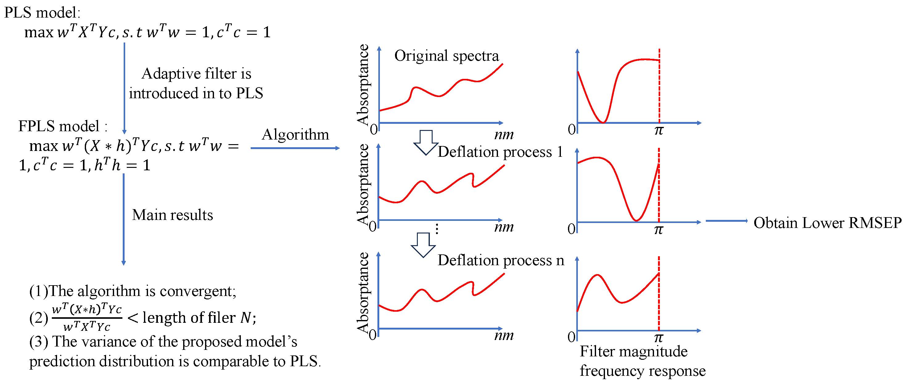
In conclusion, while existing methods provide valuable enhancements to PLS regression, they face significant challenges, especially in handling high-dimensional, noisy, and multimodal data. To address these issues, a novel PLS model that incorporates adaptively learned filters is introduced. This approach dynamically adjusts during the modeling process to better fit the data characteristics, thereby improving both the robustness and predictive performance of the model. The proposed method is summarized in Figure 1.

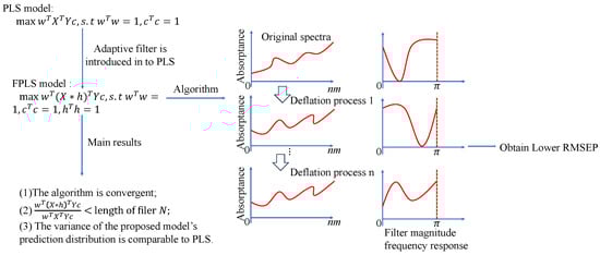
Figure 1. Flow chart of the proposed method.

The introduction of adaptive filters within PLS models marks a significant advancement in addressing these challenges. By integrating adaptive filtering directly into the PLS framework, this novel approach not only mitigates noise but also dynamically selects features most relevant to the predictive task at hand. Unlike static preprocessing methods where filters are applied prior to modeling, or probabilistic PLS models which assume certain data distributions, the proposed model learns filters adaptively during the model’s construction phase. This adaptive learning process optimizes filter parameters concurrently with loading and score matrices, leading to enhanced suppression of noise, effective feature selection, and ultimately superior model performance. The adaptability of the filters allows for a more flexible and efficient handling of complex datasets, ensuring that the model remains robust and accurate even in the presence of non-Gaussian and multimodal data characteristics. Thus, embedding adaptive filters within PLS models represents a crucial step forward in improving both the interpretability and predictivity of PLS models, setting a new standard for handling high-dimensional and noisy data.

3. Filter Learning-Based Partial Least Square (FPLS) Regression and Algorithm

Assuming $X\in R^{n\times m}$ and $Y\in R^{n\times p}$ are centered predictor and response matrices, the PLS model finds two direction vectors, $w\in R^{m\times 1}$ and $c\in R^{p\times 1}$, that satisfy [26]

$$\begin{array}{c}max{w}^T{X}^{T}Yc,s.t{w}^{T}w=1,c^{T}c=1\hfill \end{array}$$

(1)

If X contains noise, the filter should be adaptively learned, and the proposed filter PLS model can be expressed as

$$\begin{array}{cc}\hfill & max{w}^T{(X\ast h)}^{T}Yc,s.t{w}^{T}w=1,c^{T}c=1,h^{T}h=1\hfill \end{array}$$

(2)

where $h\in R^{1\times N}$ represents the filter, and the convolution operation * can be effectively carried out using matrix multiplication.

$$\begin{array}{c}\hfill X\ast h=XH=X\left[\begin{array}{cccc}{h}_1& 0& \dots & 0\\ h_2& h_1& \dots & 0\\ ⋮& ⋮& \dots & 0\\ h_N& h_{N-1}& \dots & 0\\ 0& h_N& \dots & 0\\ ⋮& ⋮& \dots & ⋮\\ 0& 0& \dots & h_1\\ ⋮& ⋮& \dots & ⋮\\ 0& 0& \dots & h_N\end{array}\right]\end{array}$$

(3)

where $H\in R^{m\times (m+1-N)}$, $XH\in R^{n\times (m+1-N)}$. In this model, we can extend X to an $n\times (m+N-1)$ matrix with zero padding. Then, H can be defined as an $R^{(m+N-1)\times m}$ matrix. Alternatively, we can define w as an $(m+1-N)\times 1$ vector. The proposed model can be rewritten as

$$\begin{array}{c}max{w}^T{\left(XH\right)}^{T}Yc,s.t{w}^{T}w=1,c^{T}c=1,\sum _{i=1}^N{h}_i^2=1\hfill \end{array}$$

(4)

3.1. Algorithm

For matrix H, we have

$$\begin{array}{c}\hfill H=h_1\left[\begin{array}{cccc}1& 0& \dots & 0\\ 0& 1& \dots & 0\\ ⋮& & \mathrm{\ddots }& \\ 0& & & 1\\ ⋮\\ 0& 0& 0& 0\end{array}\right]+h_2\left[\begin{array}{cccc}0& 0& \dots & 0\\ 1& 0& \dots & 0\\ ⋮& & \ddots \\ 0& 0& \dots & 1\\ ⋮\\ 0& 0& 0& 0\end{array}\right]+h_N\left[\begin{array}{cccc}0& 0& \dots & 0\\ ⋮& & \dots \\ 1& 0& 0& 0\\ ⋮& \ddots & \dots & 0\\ 0& 0& 1& 0\\ 0& 0& 0& 1\end{array}\right]=\sum _{i=1}^N{h}_i{C}_i\end{array}$$

(5)

We ultimately rewrite the proposed model as

$$\begin{array}{c}max{w}^T{\left(X\sum _{i=1}^N{h}_i{C}_i\right)}^{T}Yc,s.t{w}^{T}w=1,c^{T}c=1,\sum _{i=1}^N{h}_i^2=1\hfill \end{array}$$

(6)

Using Lagrange multiplier, we have

$$\begin{array}{ccc}\hfill L& =& w^T{\left(X\sum _{i=1}^N{h}_i{C}_i\right)}^{T}Yc-{\lambda }_1(w^{T}w-1)-{\lambda }_2(c^{T}c-1)-{\displaystyle \frac{1}{2}}{\lambda }_3(h^{T}h-1)\hfill \end{array}$$

(7)

$$\begin{array}{ccc}\hfill {\displaystyle \frac{\partial L}{\partial w}}& =& {\left(X\sum _{i=1}^N{h}_i{C}_i\right)}^{T}Yc-2{\lambda }_{1}w=0\hfill \end{array}$$

(8)

$$\begin{array}{ccc}\hfill {\displaystyle \frac{\partial L}{\partial c}}& =& Y^T\left(X\sum _{i=1}^N{h}_i{C}_i\right)w-2{\lambda }_{2}c=0\hfill \end{array}$$

(9)

$$\begin{array}{ccc}\hfill {\displaystyle \frac{\partial L}{\partial h_i}}& =& w^T{\left(X{C}_i\right)}^{T}Yc-{\lambda }_3{h}_i=0\hfill \end{array}$$

(10)

$$\begin{array}{ccc}\hfill {\displaystyle \frac{\partial L}{\partial {\lambda }_1}}& =& -(w^{T}w-1)=0\hfill \end{array}$$

(11)

$$\begin{array}{ccc}\hfill {\displaystyle \frac{\partial L}{\partial {\lambda }_2}}& =& -(c^{T}c-1)=0\hfill \end{array}$$

(12)

$$\begin{array}{ccc}\hfill {\displaystyle \frac{\partial L}{\partial {\lambda }_3}}& =& -(h^{T}h-1)=0\hfill \end{array}$$

(13)

Multiply both sides of Equations (8) and (9) by $w^T$ and $c^T$, respectively. According to Equations (11) and (12), $w^{T}w=1$, $c^{T}c=1$; thus, we have

$$\begin{array}{ccc}\hfill w^T{\left(X\sum _{i=1}^N{h}_i{C}_i\right)}^{T}Yc& =& 2{\lambda }_1\hfill \end{array}$$

(14)

$$\begin{array}{ccc}\hfill c^T{Y}^T\left(X\sum _{i=1}^N{h}_i{C}_i\right)w& =& 2{\lambda }_2\hfill \end{array}$$

(15)

A scalar is equal to its transpose; thus, ${\displaystyle w^T{\left(X\sum _{i=1}^N{h}_i{C}_i\right)}^{T}Yc=c^T{Y}^T\left(X\sum _{i=1}^N{h}_i{C}_i\right)}$, namely, $2{\lambda }_1=2{\lambda }_2=\eta$. Based on Equation (9), we can derive that $Y^T\left(X{\sum }_{i=1}^N{h}_i{C}_i\right)w=\eta c$. Substituting it into Equation (8) gives us the following:

$$\begin{array}{c}\hfill {\left(X\sum _{i=1}^N{h}_i{C}_i\right)}^{T}Y{Y}^T\left(X\sum _{i=1}^N{h}_i{C}_i\right)w={\eta }^{2}w,\end{array}$$

(16)

Similarly, we have

$$\begin{array}{c}\hfill Y^T\left(X\sum _{i=1}^N{h}_i{C}_i\right){\left(X\sum _{i=1}^N{h}_i{C}_i\right)}^{T}c={\eta }^{2}c\end{array}$$

(17)

According to (10), ${\displaystyle \sum _{i=1}^N{w}^T{\left(X{h}_i{C}_i\right)}^{T}Yc-{\lambda }_3{h}_i^2=0}$, namely ${\displaystyle \sum _{i=1}^N{w}^T{\left(X{h}_i{C}_i\right)}^{T}Yc={\lambda }_3\sum _{i=1}^N{h}_i^2={\lambda }_3}$. Thus, we have

$$\begin{array}{c}\hfill h_i={\displaystyle \frac{w^T{\left(X{C}_i\right)}^{T}Yc}{w^T{\left({\displaystyle X\sum _{i=1}^N{h}_i{C}_i}\right)}^{T}Yc}}\end{array}$$

(18)

The proposed FPLS algorithm is shown in Algorithm 1.

Algorithm 1 FPLS

Input: Predictor matrix $X\in R^{n\times m}$, response matrix $Y\in R^{n\times p}$, initial filter $h=[h_1,\cdots ,h_N]\in R^{1\times N}$.   Step 1: Predictor matrix is calculated as $XH$, and then employ traditional PLS algorithm to build the regression model, resulting in the acquisition of w and c;   Step 2: Updating i-th element of filter h to $h_i={\displaystyle \frac{w^T{\left(X{C}_i\right)}^{T}Yc}{w^T{\left({\displaystyle X\sum _{i=1}^N{h}_i{C}_i}\right)}^{T}Yc}},i=1,\cdots ,N$;   Step 3: Performing the deflation process;   Step 4: Repeat Step 1–3 t times and obtain $w_j,c_j,h_j=[h_{1j},\cdots ,h_{Nj}],j=1,\cdots ,t$;

3.2. Convergence Analysis

If c and h are fixed, we define $L_w$ as

$$\begin{array}{ccc}\hfill L_w(w,c,H)& =& w^T{\left(X\sum _{i=1}^N{h}_i{C}_i\right)}^{T}Yc-{\lambda }_1(w^{T}w-1)\hfill \end{array}$$

(19)

In the t-th step, we find $w_t$ that maximizes $L_w(w,c,H)$ and in the $(t+1)$-th step, we can determine $w_{t+1}$, such that

$$\begin{array}{c}\hfill w_{t+1}^T{\left(X\sum _{i=1}^N{h}_i{C}_i\right)}^{T}Yc\ge w_t^T{\left(X\sum _{i=1}^N{h}_i{C}_i\right)}^{T}Yc\end{array}$$

(20)

According to Equation (8), $w=\left({\left({\displaystyle X\sum _{i=1}^N{h}_i{C}_i}\right)}^{T}Yc/2{\lambda }_1\right)$, then

$$\begin{array}{cc}\hfill {\left({\left({\displaystyle X\sum _{i=1}^N{h}_i{C}_i}\right)}^{T}Yc/2{\lambda }_1\right)}^T{\left(X\sum _{i=1}^N{h}_i{C}_i\right)}^{T}Yc& \ge w_{t+1}^T{\left(X\sum _{i=1}^N{h}_i{C}_i\right)}^{T}Yc\hfill \\ & \ge w_t^T{\left(X\sum _{i=1}^N{h}_i{C}_i\right)}^{T}Yc\hfill \end{array}$$

(21)

Similarly, we have

$$\begin{array}{cc}\hfill w{\left(X\sum _{i=1}^N{h}_i{C}_i\right)}^{T}Y{\left(Y^T\left({\displaystyle X\sum _{i=1}^N{h}_i{C}_i}\right)w/2{\lambda }_2\right)}^T& \ge w^T{\left(X\sum _{i=1}^N{h}_i{C}_i\right)}^{T}Y{c}_{t+1}\hfill \\ & \ge w^T{\left(X\sum _{i=1}^N{h}_i{C}_i\right)}^{T}Y{c}_t\hfill \end{array}$$

(22)

$$\begin{array}{cc}\hfill w^T{\left(X\sum _{i=1}^N\left(w^T{\left(X{C}_i\right)}^{T}Yc/2{\lambda }_3\right)C_i\right)}^{T}Yc& \ge w^T{\left(X\sum _{i=1}^N{h}_{t+1,i}{C}_i\right)}^{T}Yc\hfill \\ & \ge w^T{\left(X\sum _{i=1}^N{h}_{t,i}{C}_i\right)}^{T}Yc\hfill \end{array}$$

(23)

3.3. Model Performance Analysis

It is difficult to directly analyze the model because it involves the eigenvalues and eigenvectors of $X^{T}Y{Y}^{T}X$. In this section, for simplicity without losing generality, we consider the PLS-one model. Suppose $X=\left[x_{ij}\right]\in R^{n\times m}$, $y={\left[y_1,\cdots ,y_n\right]}^T$, $w={\left[w_1,\cdots ,w_m\right]}^T$. The Lagrangian function is then constructed as

$$\begin{array}{c}\hfill \mathcal{L}=w^T{X}^{T}Y-\lambda (w^{T}w-1)=\sum _{i=1}^n{y}_i\sum _{j=1}^m{x}_{ij}{w}_j-\lambda (w^{T}w-1)\end{array}$$

(24)

Calculating the partial derivative of $\mathcal{L}$ with respect to $w_i$, we have

$$\begin{array}{c}\hfill {\displaystyle \frac{\partial \mathcal{L}}{\partial w_1}}=\sum _{i=1}^n{x}_{i1}{y}_i-2\lambda w_1=0,\cdots {\displaystyle \frac{\partial \mathcal{L}}{\partial w_m}}=\sum _{i=1}^n{x}_{im}{y}_i-2\lambda w_m=0\end{array}$$

(25)

Thus,

$$\begin{array}{c}\hfill w^T{X}^{T}Y\propto Y^{T}X{X}^{T}Y=\sum _{i=1}^m{\left(\sum _{j=1}^n{y}_j{x}_{ji}\right)}^2\end{array}$$

(26)

If a filter with length N is employed to filter X, without loss of generality, the first term of ${\sum }_{i=1}^m{\left({\sum }_{j=1}^n{y}_j{x}_{ji}\right)}^2$ is equal to $(y_1(h_1{x}_{11}+\cdots$$+h_N{x}_{1N}{)+\cdots +y_n(h_1{x}_{n1}+\cdots +h_N{x}_{nN}))}^2$. The spectrum is usually smooth in a small neighborhood. If $h_i$ has the same sign for all $i=1,\cdots ,N$, then

$$\begin{array}{c}\hfill max{y}_1(h_1{x}_{11}+\cdots +h_N{x}_{1N})=max{y}_1\sum _{i=1}^N{h}_i{x}_{11}=\sqrt{N}{y}_1{x}_{11}\end{array}$$

(27)

when $h_i={\displaystyle \frac{1}{\sqrt{N}}}$ for all $i=1,2,\cdots ,N$. By appropriately choosing N, we can approximate $max{w}^T{(X\ast h)}^{T}Y$ as $N{w}^T{X}^{T}Y$. Assuming $max{w}^T{X}^{T}Y>0$, we have $0<w^T{(X\ast h)}^{T}Y<N{w}^T{X}^{T}Y$, which can be rewritten as

$$\begin{array}{c}\hfill 0<{\displaystyle \frac{w^T{(X\ast h)}^{T}Y}{w^T{X}^{T}Y}}<N\end{array}$$

(28)

The closer the filter h coefficients are, the closer ${\displaystyle \frac{w^T{(X\ast h)}^{T}Y}{w^T{X}^{T}Y}}$ is to N.

For the proposed model shown in Equation (2), we adopt a similar approach for analysis. The filtered X is defined as $X^{\prime }$, where the term $x_{ij}^{\prime }$ is given by ${\sum }_{k=i}^N{h}_k{x}_{(i+k)j}$. When N is relatively small, considering the smoothness in the neighborhood, we approximately assume that ${\sum }_{k=i}^N{h}_k{x}_{(i+k)j}\approx x_{ij}{\sum }_{k=i}^N{h}_k$. When $h_k={\displaystyle \frac{1}{\sqrt{N}}}$ for $k=1,2,\cdots ,N$, $x_{ij}{\sum }_{k=i}^N{h}_k$ obtains the maximum value $\sqrt{N}{x}_{ij}$. Thus, $X^{\prime }=\sqrt{N}X$, $X^{\prime T}Y{Y}^T{X}^{\prime }w={\left(\sqrt{N}X\right)}^{T}Y{Y}^T\left(\sqrt{N}X\right)w=N{X}^{T}Y{Y}^{T}Xw={\lambda }_{filtered}w$. So, we have ${\displaystyle \frac{{\lambda }_{filtered}}{\lambda }}=N$ and, similarly, we have

$$\begin{array}{c}\hfill 0<{\displaystyle \frac{w^T{(X\ast h)}^{T}Yc}{w^T{X}^{T}Yc}}<N\end{array}$$

(29)

Obviously, the vector w must differ before and after filtering, and the above analysis is also approximate to a certain extent.

The prediction variance can be analyzed using probabilistic methods. Let u represent a hidden variable; the relation between x and u is $x=Pu+{\mu }_x+\xi$ and $y=Cu+{\mu }_y+\eta$, where $\xi$ and $\eta$ represent Gaussian noise, satisfying $\xi \sim N(0,{\sigma }_x^{2}I)$ and $\eta \sim N(0,{\sigma }_y^{2}I)$, respectively; ${\mu }_x$ and ${\mu }_y$ represent the mean vectors of X and Y, respectively; and P and C represent the transformation matrices for X and Y, respectively. The variance of prediction distribution is $C{\sigma }_x^2{(P^{T}P+{\sigma }_x^2)}^{-1}{C}^T+{\sigma }_y^{2}I$, which is related to the inverse of matrix $(P^{T}P+{\sigma }_x^{2}I)$[19]. Assuming $x=[x_1,x_2,\cdots ,x_m]$, the filtered vector $x^{\prime }$ can be approximated as $x^{\prime }=\left[{\sum }_{i=1}^N{h}_i{x}_i,{\sum }_{i=1}^N{h}_i{x}_{i+1},\cdots ,{\sum }_{i=1}^N{h}_i{x}_{i+m-1}\right]\approx \left[x_1{\sum }_{i=1}^N{h}_i,x_2{\sum }_{i=1}^N{h}_i,\cdots ,\right.$$\left.x_m{\sum }_{i=1}^N{h}_i\right]$, and the approximate variance of $x^{\prime }$ is given by ${\sum }_{i=1}^N{h}_i^2{\sigma }_x^{2}I={\sigma }_x^{2}I$. For example, in the two-dimensional case, suppose $P=[p_1,p_2;p_3,p_4]$ and $C=[c_1,c_2]$. Then, the variance of prediction is

$$\begin{array}{c}{\displaystyle \frac{(c_1^2+c_2^2){\sigma }_x^4+\left[c_1^2(p_1^2+p_4^2)+c_2^2(p_1^2+p_3^2)\right]{\sigma }_x^2+{\sigma }_y^2}{{\sigma }_x^4+(p_1^2+p_2^2+p_3^2+p_4^2){\sigma }_x^2+{(p_1{p}_4-p_2{p}_3)}^2}}\hfill \\ \approx (c_1^2+c_2^2)+\{\left[c_1^2(p_1^2+p_4^2)+c_2^2(p_1^2+p_3^2)\right]-(c_1^2+c_2^2)(p_1^2+p_2^2+p_3^2+p_4^2)\}{\sigma }_x^{-2}\hfill \\ +({\sigma }_y^2-(c_1^2+c_2^2){(p_1{p}_4-p_2{p}_3)}^2-(p_1^2+p_2^2+p_3^2+p_4^2)\{\left[c_1^2(p_1^2+p_4^2)+c_2^2(p_1^2+p_3^2)\right]\hfill \\ -(c_1^2+c_2^2)(p_1^2+p_2^2+p_3^2+p_4^2)\left\}\right){\sigma }_x^{-4}\hfill \end{array}$$

(30)

If a filter with length N is employed, the filtered signal is approximately ${\sum }_{i=1}^N{h}_i{x}_i$, thus the variance is ${\sum }_{i=1}^N{h}_i^2{\sigma }_x^{2}I={\sigma }_x^{2}I$. Choosing an appropriate N can ensure that the prediction variance of the proposed model is essentially consistent with that of PLS.

4. Experiment and Analysis

In this section, we compare the accuracy of the proposed and alternative methods with four public datasets: Corn, Octane, Mango, and Soil Infrared Spectra datasets. These databases are commonly employed to evaluate regression-based analysis. In our experiments, the accuracy is calculated using Root Mean Squared Error of Prediction (RMSEP). The experiments were implemented with a laptop with a 2.80 GHz i7 processor, 16.0 GB RAM and Win10 system. In our experiments, we compared our FPLS with eight other methods: PLS [27], Orthogonal Signal Correction + PLS (OSCPLS) [13], Variance Constrained PLS (VCPLS) [28], Powered PLS (PoPLS) [29], Low-pass Filter + PLS (LoPLS), Direct Orthogonal Signal Correction + PLS (DOSC) [15], Orthogonal Projections to Latent Structures (OPLS) [14], Multiplicative Signal Correction (MSC), Standard Normal Variate (SNV), Savitzky–Golay (SG) Filtering, and Least Absolute Shrinkage and Selection Operator (Lasso) [30]. In our experiments, we randomly selected 70% of the sample as the training set, and the remaining 30% as the test set. We repeated the experiment 300 times.

In our experiment, OSCPLS, OPLS, DOSC, and VCPLS settings are accordance with reference [28]. LoPLS is an unsupervised method, and thus, we specify the low-pass filter as $h=\left[1/\sqrt{2},1/\sqrt{2}\right]$. The coefficients $1/\sqrt{2}$ ensure that the filter preserves signal energy without excessive amplification or attenuation. It smooths out high-frequency noise while retaining low-frequency components of the signal, making it effective for denoising. The filter is computationally efficient, using just two coefficients, which is suitable for real-time processing. The equal weighting of current and previous samples minimizes phase distortion.

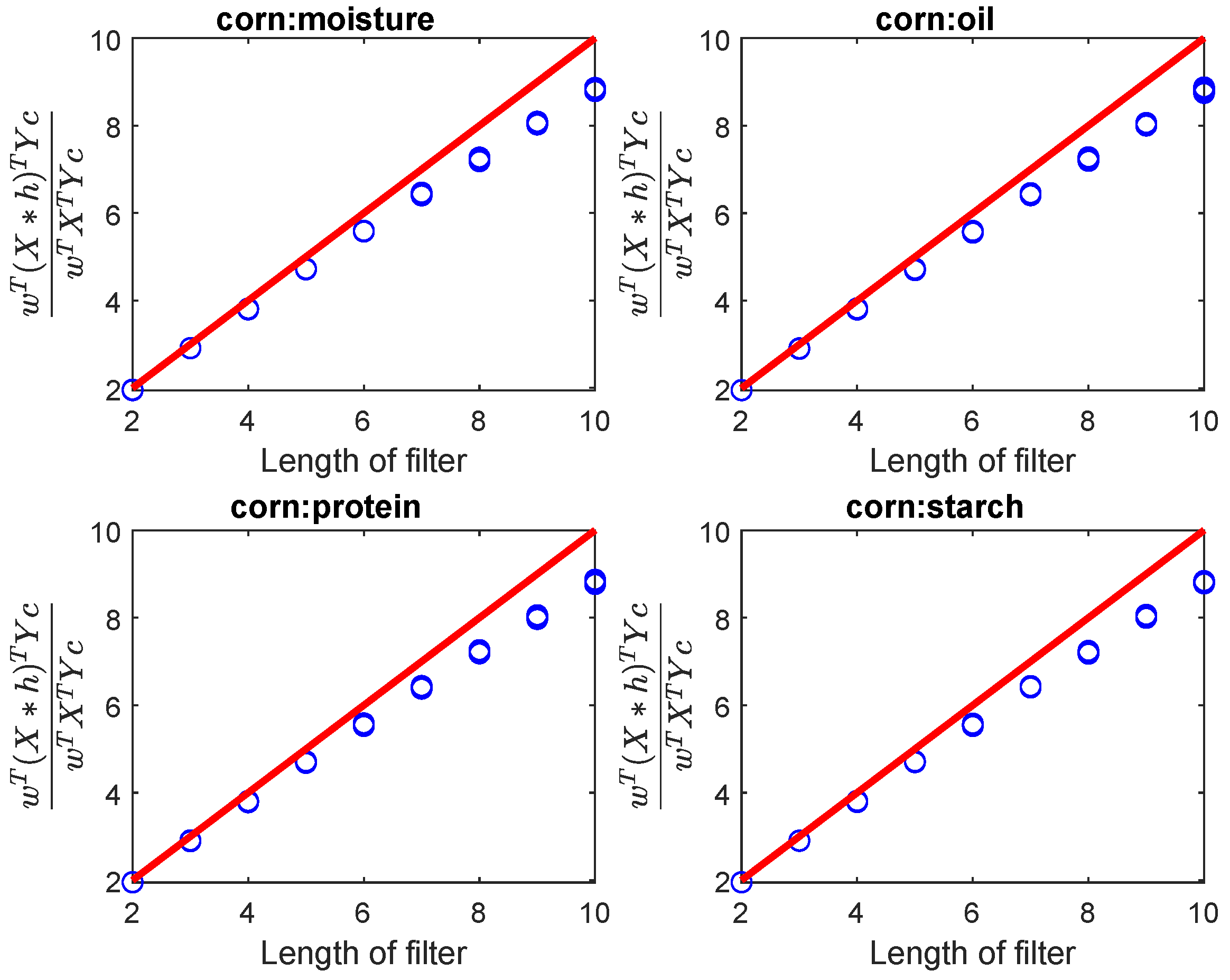
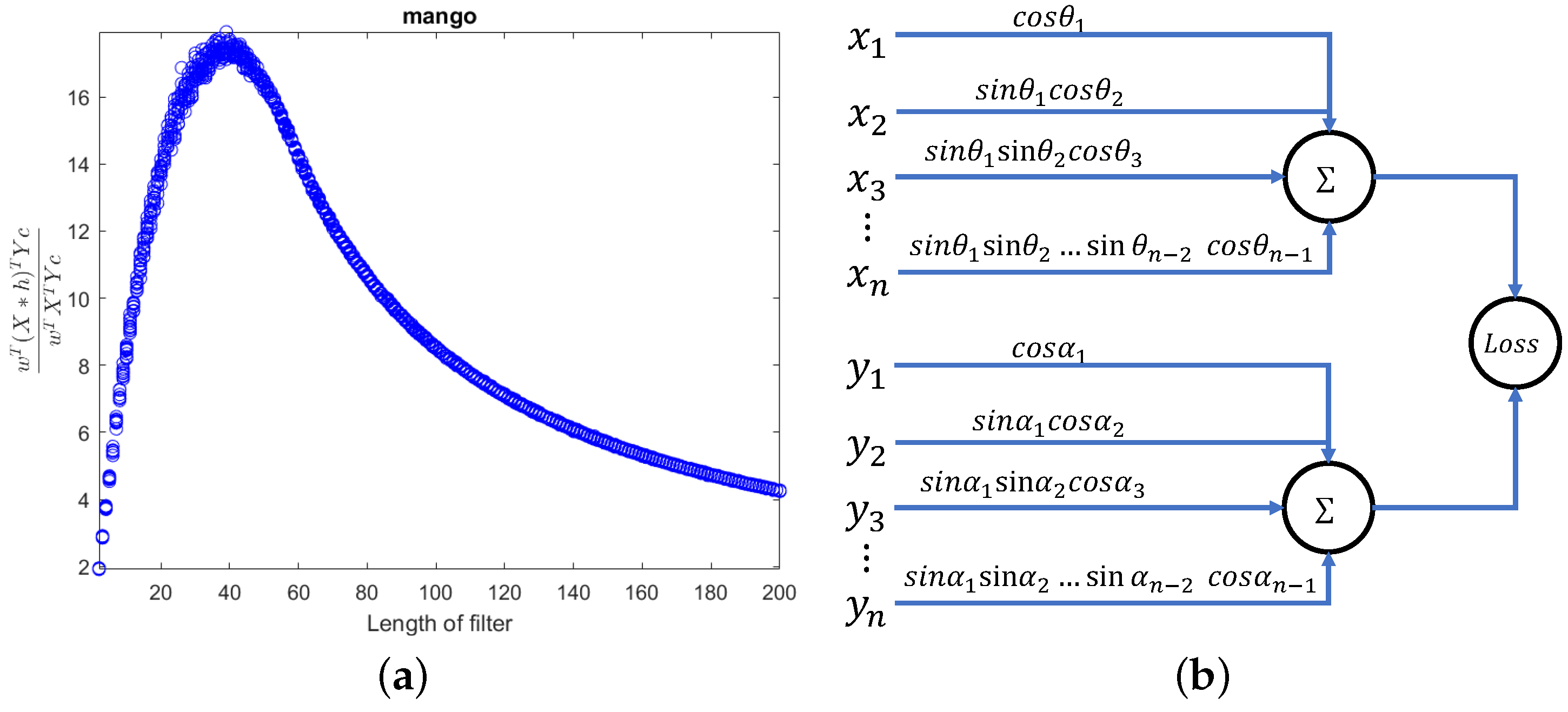
In the theoretical analysis of FPLS, the local smoothness of the spectra was considered, which means that the length of the filter could not be too long. As N increases, ${\displaystyle \frac{w^T{(X\ast h)}^{T}Yc}{w^T{X}^{T}Yc}}$ gradually deviates from N, because smoothness of spectra cannot be guaranteed after N increases, as shown in Figure 2. Thus, in our experiments, the range of length of filter was set to $[2,3,4]$. The conclusions drawn from filter length selection on the Octane, Mango, and soil datasets are consistent and will not be repeated here. The optimal number of components for the FPLS was determined through 10-fold cross-validation. For the SGFilter method, the order and frame length were also determined with 10-fold cross-validation.

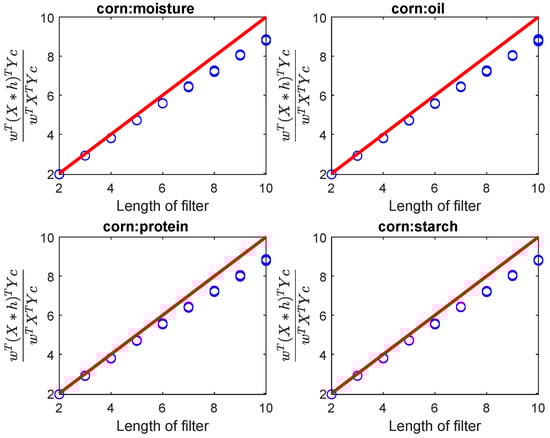
Figure 2. As the length of the filter increases, the ratio ${\displaystyle \frac{w^T{(X\ast H)}^{T}Yc}{w^T{X}^{T}Yc}}$ varies. Due to the inability to satisfy the local smoothness of the spectral signal as the filter length increases, ${\displaystyle \frac{w^T{(X\ast H)}^{T}Yc}{w^T{X}^{T}Yc}}$ gradually moves away from upper bond N. The response Y represents the values for moisture, oil, protein, and starch, respectively.

We compared the performance of different models in terms of RMSEP on the testing set. RMSEP is defined as the square root of the mean squared prediction error, which measures the average magnitude of the errors between predicted and actual values.

$$\begin{array}{c}\hfill RMSEP=\sqrt{{\displaystyle \frac{1}{n}}{\displaystyle \sum _i^n}{(y_i-{\widehat{y}}_i)}^2}=\sqrt{{\displaystyle \frac{1}{n}}{\displaystyle \sum _i^n}{({\widehat{y}}_i-y_i)}^2}\end{array}$$

(31)

The prediction and response of the i-th observation are denoted as ${\widehat{y}}_i$ and $y_i$, respectively. The number of the test set is n. The variance of prediction is ${\displaystyle \frac{1}{n}}{\sum }_{i=1}^n{\left({\widehat{y}}_i-{\displaystyle \frac{1}{n}}{\sum }_{i=1}^n{\widehat{y}}_i\right)}^2$.

We also compare the performance of different models in terms of Cosine Similarity (CS) on the testing set. It is a commonly used method to measure the similarity between two non-zero vectors.

$$\begin{array}{c}\hfill CS(\widehat{\mathit{y}},\mathit{y})={\displaystyle \frac{{\mathit{y}}^T\widehat{\mathit{y}}}{\parallel \mathit{y}\parallel \parallel \widehat{\mathit{y}}\parallel }}={\displaystyle \frac{{\widehat{\mathit{y}}}^T\mathit{y}}{\parallel \mathit{y}\parallel \parallel \widehat{\mathit{y}}\parallel }}\end{array}$$

(32)

$\widehat{\mathit{y}}\in R^{n\times 1}$ and $\mathit{y}\in R^{n\times 1}$ represent the predicted result and the reference, respectively. We then discussed the range of $CS$ when $RMSEP$ is given, as well as the range of $RMSEP$ when $CS$ is provided. For convenience of description, let RMSEP be denoted as $\alpha$. According to Equation (31), $\widehat{\mathit{y}}$ lies on a hypersphere centered at $\mathit{y}$ with radius $\sqrt{n}\alpha$. It is evident that the minimum value of CS is ${\displaystyle \frac{\sqrt{{\parallel \mathit{y}\parallel }^2-nRMSE{P}^2}}{\parallel \mathit{y}\parallel }}$. Therefore, the range of CS is

$$\begin{array}{c}\hfill \left[-1,-{\displaystyle \frac{\sqrt{{\parallel \mathit{y}\parallel }^2-nRMSE{P}^2}}{\parallel \mathit{y}\parallel }}\right]\bigcup \left[{\displaystyle \frac{\sqrt{{\parallel \mathit{y}\parallel }^2-nRMSE{P}^2}}{\parallel \mathit{y}\parallel }},1\right]\end{array}$$

(33)

Similarly, we can analyze how the upper bound of $RMSEP$ changes when CS varies. $CS(\widehat{\mathit{y}},\mathit{y})={\displaystyle \frac{{\mathit{y}}^T\widehat{\mathit{y}}}{\parallel \mathit{y}\parallel \parallel \widehat{\mathit{y}}\parallel }}\Rightarrow {\mathit{y}}^T\widehat{\mathit{y}}=CS\parallel \mathit{y}\parallel \parallel \widehat{\mathit{y}}\parallel$. Usually, $CS$ is not equal to zero and, assuming that $\widehat{\mathit{y}}=\mathit{y}+\Delta \mathit{y}(\Delta \mathit{y}\to 0)$, this means that $\parallel \widehat{\mathit{y}}\parallel \approx {\displaystyle \frac{\parallel \mathit{y}\parallel }{CS}}$. We thus have

$$\begin{array}{cc}\hfill RMSE{P}^2& ={\displaystyle \frac{{\parallel \mathit{y}\parallel }^2+{\parallel \widehat{\mathit{y}}\parallel }^2-2{\mathit{y}}^T\widehat{\mathit{y}}}{n}}={\displaystyle \frac{{\parallel \mathit{y}\parallel }^2+\parallel \widehat{\mathit{y}}{\parallel }^2-2CS\parallel \mathit{y}\parallel \parallel \widehat{\mathit{y}}\parallel }{n}}\hfill \\ & \le {\displaystyle \frac{{\parallel \mathit{y}\parallel }^2+{\parallel \widehat{\mathit{y}}\parallel }^2-2CS\frac{\parallel \mathit{y}\parallel \parallel \widehat{\mathit{y}}\parallel }{\parallel \mathit{y}\parallel +\parallel \widehat{\mathit{y}}\parallel }}{n}}(\parallel \mathit{y}\parallel +\parallel \widehat{\mathit{y}}\parallel \ge 1)\hfill \\ & ={\displaystyle \frac{{\parallel \mathit{y}\parallel }^2+\frac{{\parallel \mathit{y}\parallel }^2}{C{S}^2}-2CS\frac{\parallel \mathit{y}\parallel \frac{\parallel \mathit{y}\parallel }{CS}}{\parallel \mathit{y}\parallel +\frac{\parallel \mathit{y}\parallel }{CS}}}{n}}={\displaystyle \frac{{\parallel \mathit{y}\parallel }^2+\frac{{\parallel \mathit{y}\parallel }^2}{C{S}^2}-2\frac{\parallel \mathit{y}\parallel CS}{CS+1}}{n}}\hfill \\ & ={\displaystyle \frac{{\parallel \mathit{y}\parallel }^2+\frac{{\parallel \mathit{y}\parallel }^2}{C{S}^2}-2\frac{\parallel \mathit{y}\parallel }{1+\frac{1}{CS}}}{n}}\hfill \end{array}$$

(34)

We note that ${\displaystyle \frac{{\parallel \mathit{y}\parallel }^2+\frac{{\parallel \mathit{y}\parallel }^2}{C{S}^2}-2\frac{\parallel \mathit{y}\parallel }{1+\frac{1}{CS}}}{n}}$ decreases as $CS$ increases.

$$\begin{array}{c}\hfill RMSEP\le \sqrt{{\displaystyle \frac{{\parallel \mathit{y}\parallel }^2+\frac{{\parallel \mathit{y}\parallel }^2}{C{S}^2}-2\frac{\parallel \mathit{y}\parallel CS}{1+CS}}{n}}}\end{array}$$

(35)

On the other hand,

$$\begin{array}{cc}\hfill {\displaystyle \frac{{\parallel \mathit{y}\parallel }^2+\parallel \widehat{\mathit{y}}{\parallel }^2-2CS\parallel \mathit{y}\parallel \parallel \widehat{\mathit{y}}\parallel }{n}}& \ge {\left.{\displaystyle \frac{{\parallel \mathit{y}\parallel }^2+\parallel \widehat{\mathit{y}}{\parallel }^2-2CS\parallel \mathit{y}\parallel \parallel \widehat{\mathit{y}}\parallel }{n}}\right|}_{\parallel \widehat{\mathit{y}}\parallel =CS\parallel \mathit{y}\parallel }\hfill \\ & ={\displaystyle \frac{{\parallel \mathit{y}\parallel }^2(1-C{S}^2)}{n}}\hfill \end{array}$$

(36)

Therefore, we have

$$\begin{array}{c}\hfill {\displaystyle \frac{{\parallel \mathit{y}\parallel }^2(1-C{S}^2)}{n}}\le RMSEP\le \sqrt{{\displaystyle \frac{{\parallel \mathit{y}\parallel }^2+\frac{{\parallel \mathit{y}\parallel }^2}{C{S}^2}-2\frac{\parallel \mathit{y}\parallel CS}{1+CS}}{n}}}\end{array}$$

(37)

If ${\parallel \mathit{y}\parallel }^2<nRMSE{P}^2$, CS$\in [-1,1]$. At this moment, $\sqrt{n}RMSEP-\parallel \mathit{y}\parallel <RMSEP<\sqrt{n}RMSEP$.

4.1. Corn Dataset Analysis

This set comprises 80 Corn samples, and the wavelength range is 1100–2498 nm with 2 nm intervals. Each spectrum is a 700-dimensional vector (http://www.eigenvector.com/data/Corn/index.html (accessed on 13 January 2023)). In our experiments, the analysis focuses on moisture, oil, protein, and starch. The corresponding ranges for each parameter are as follows: moisture (9.377–10.993%), oil (3.088–3.832%), protein (7.654–9.711%), and starch (62.826–66.472%). After obtaining the parameters, the spectra are filtered. Then, the regression model is established using PLS. In the analysis of Corn data, the best mean RMSEP and prediction variances of FPLS, PLS, OSCPLS, VCPLS, PoPLS, LoPLS, DOSC, OPLS, MSC, SNV, SGFilter, and Lasso are presented in Table 1. The numbers in parentheses next to RMSEP indicate the optimal number of components used in the respective regression model.

Table 1. Corn moisture, oil, protein, and starch prediction results in terms of RMSEP and variance.

Method	Moisture		Oil		Protein		Starch
	RMSEP	Variance	RMSEP	Variance	RMSEP	Variance	RMSEP	Variance
FPLS	0.0977 (20)	0.0007	0.0601 (20)	0.0002	0.1069 (20)	0.0010	0.2521 (20)	0.0045
PLS	0.1516 (10)	0.0007	0.1026 (7)	0.0002	0.1583 (10)	0.0011	0.3929 (9)	0.0045
OSCPLS	0.1840 (1)	0.0006	0.1299 (1)	0.0003	0.1788 (2)	0.0012	0.5059 (4)	0.0152
VCPLS	0.1498 (1)	0.0003	0.1027 (1)	0.0002	0.1549 (1)	0.0004	0.3877 (2)	0.0021
PoPLS	0.1598 (7)	0.0012	0.1085 (6)	0.0003	0.1574 (8)	0.0018	0.4301 (9)	0.0058
LoPLS	0.1516 (10)	0.0007	0.2272 (7)	0.0002	0.1583 (10)	0.0011	0.3927 (9)	0.0045
DOSC	0.1837 (1)	0.0006	0.1297 (1)	0.0003	0.1788 (2)	0.0012	0.5057 (4)	0.0154
OPLS	0.1533 (9)	0.0015	0.1029 (6)	0.0003	0.1585 (9)	0.0024	0.3926 (8)	0.0121
MSC	0.2179 (7)	0.0009	0.1067 (7)	0.0017	0.1642 (9)	0.0012	0.3843 (9)	0.0314
SNV	0.2174 (11)	0.0009	0.1067 (7)	0.0017	0.1642 (9)	0.0012	0.3896 (9)	0.0317
SGFilter	0.1533 (10)	0.0012	0.1042 (8)	0.0003	0.1569 (9)	0.0019	0.3925 (9)	0.0353
Lasso	0.1545 (1)	0.0004	0.1123 (1)	0.0002	0.1629 (1)	0.0006	0.4290 (1)	0.0041

According to Table 1, in moisture prediction, FPLS stands out with the lowest RMSEP value of 0.0977, indicating its high accuracy in predicting moisture content. This method also has a variance value of 0.0007, suggesting that its predictions are relatively stable and consistent. In contrast, methods such as MSC and SNV have higher RMSEP values of 0.2179 and 0.2174, respectively, indicating that their predictions may be less accurate compared to FPLS. Other methods, including PLS, OSCPLS, VCPLS, PoPLS, LoPLS, DOSC, OPLS, SGFilter, and Lasso, have RMSEP values that range from 0.1498 to 0.1840. These methods may have varying degrees of accuracy in predicting moisture content, depending on the specific dataset and conditions used for evaluation. FPLS and PLS have the same variance value of 0.0007, which is consistent with our previous analysis. According to Table 1, the RMSEP and variance results of these methods for oil, protein, and starch prediction are similar to the results of moisture. In conclusion, FPLS appears to be the best method for predicting moisture content.

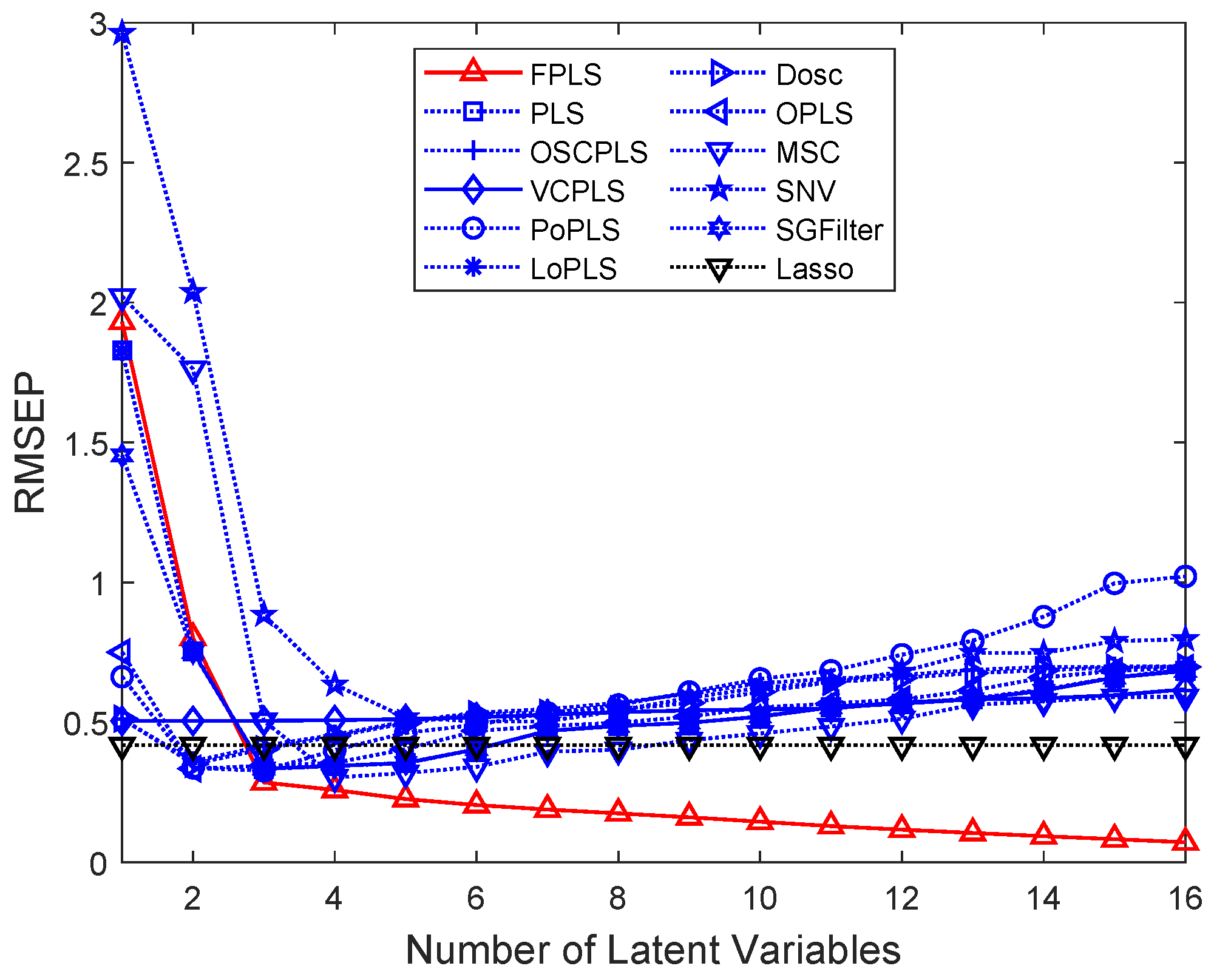
Figure 3a–d show that as the number of components increases, the RMSEP values for moisture, oil, protein, and starch prediction decrease. Regarding Lasso, it differs from the aforementioned methods; it is a variable selection method. In this figure, the horizontal axis represents the number of random experiments conducted for Lasso. Among these methods, FPLS exhibits a faster decline in RMSEP compared to other approaches. Furthermore, beyond a certain number of components, the RMSEP of FPLS becomes significantly smaller than that of other methods. Specifically, the number of components is observed to be 7 for moisture prediction, 5 for oil, and 8 for both protein and starch. These figures also validate the effectiveness of the FPLS method.

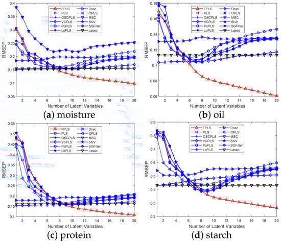
Figure 3. RMSEP values for the prediction of moisture, oil, and protein content in Corn samples using various methods, including FPLS, PLS, OSCPLS, VCPLS, PoPLS, LoPLS, DOSC, OPLS, MSC, SNV, and SGFilter, with 1 to 20 components each.

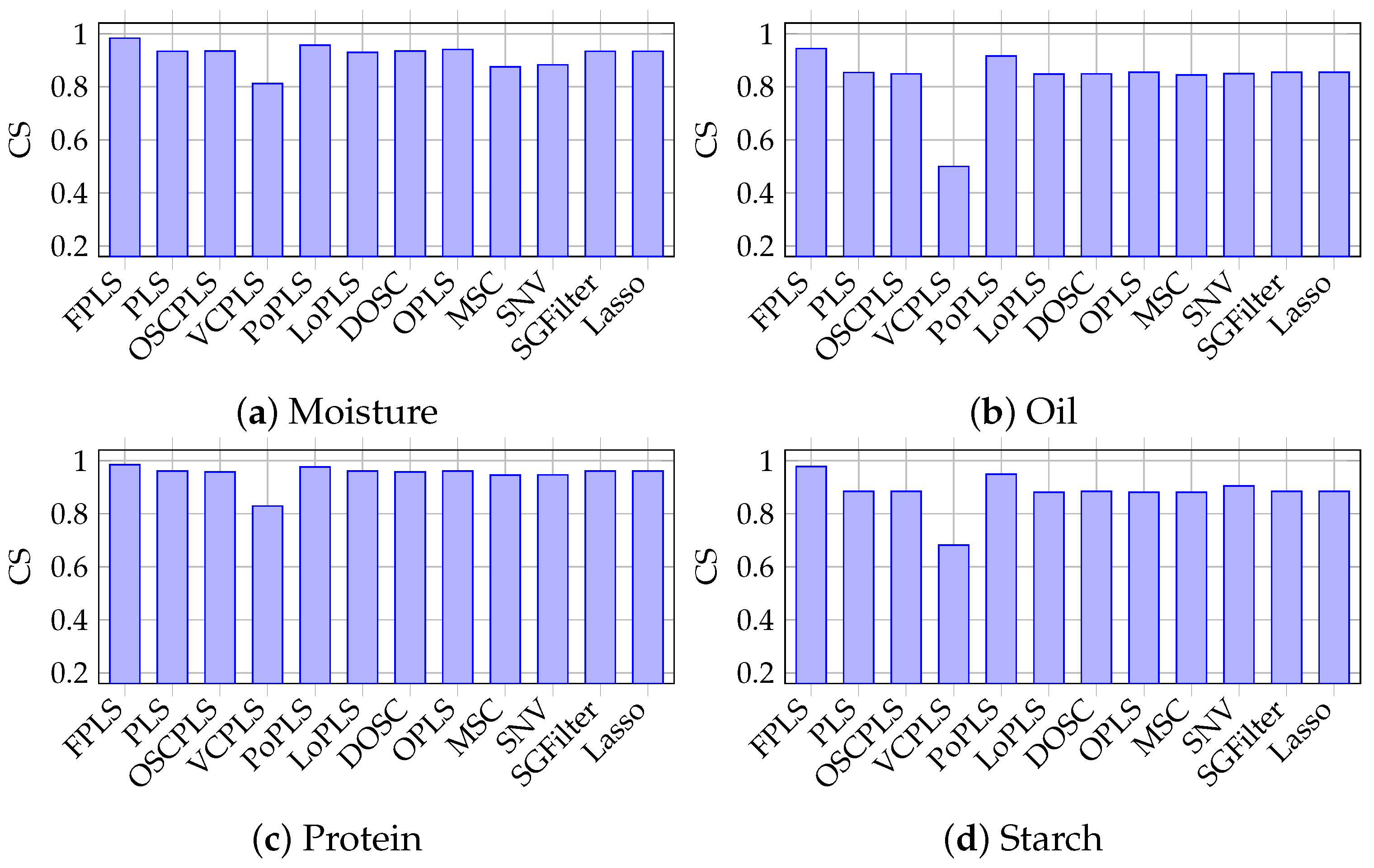
Figure 4a–d show the CS (Cosine Similarity) between the responses and predictions for moisture, oil, protein, and starch with FPLS, PLS, OSCPLS, VCPLS, PoPLS, LoPLS, DOSC, OPLS, MSC, SNV, SGFilter, and Lasso. The vertical axis represents the CS values. It can be observed that among these algorithms, FPLS has the highest CS. Furthermore, combining this with Table 1, it can be inferred that the RMSEP is small, and the CS between the predicted values and responses is high, indicating that the model possesses excellent predictive ability and generalization performance. Based on the analysis of Table 1, and Figure 3 and Figure 4, the proposed FPLS method outperforms PLS, OSCPLS, VCPLS, PoPLS, LoPLS, DOSC, OPLS, MSC, SNV, SGFilter, and Lasso in terms of RMSEP for moisture, oil, protein, and starch prediction.

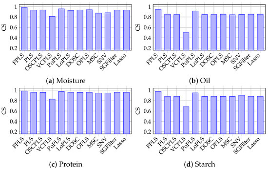
Figure 4. Cosine Similarity between prediction results and response in moisture, oil, protein, and starch prediction using FPLS, PLS, OSCPLS, VCPLS, PoPLS, LoPLS, DOSC, OPLS, MSC, SNV, SGFilter, and Lasso.

The boundaries of RMSEP and CS in predictive experiments for moisture content were analyzed, with the results presented in Table 2. According to this table, the boundaries of RMSEP and CS align with Equations (33) and (37). Similar conclusions are also drawn regarding the boundaries of RMSEP and CS in predictive experiments for oil, starch, and protein; however, for brevity, these results are not listed here.

Table 2. Upper and lower boundaries of RMSEP and CS. In this experiment on Corn moisture prediction, the lower and upper bounds of RMSEP and the lower bound of CS are provided. In this table, “Lower RMSEP” and “Upper RMSEP” denote the respective lower and upper boundaries of RMSEP, while “Lower CS” signifies the lower boundary of CS.

Method	RMSEP	CS	Lower RMSEP	Upper RMSEP	Lower CS
FPLS	0.0977	0.9834	0.0052	0.5363	0.9691
PLS	0.1516	0.9343	0.0199	0.5531	0.9237
OSCPLS	0.1840	0.9347	0.0198	0.5529	0.8854
VCPLS	0.1498	0.8124	0.0533	0.6049	0.9256
PoPLS	0.1598	0.9576	0.0130	0.5448	0.9149
LoPLS	0.1516	0.9298	0.0212	0.5547	0.9237
DOSC	0.1837	0.9347	0.0198	0.5529	0.8858
OPLS	0.1533	0.9407	0.0180	0.5507	0.9219
MSC	0.2179	0.8760	0.0365	0.5758	0.8348
SNV	0.2174	0.8828	0.0346	0.5730	0.8356
SGFilter	0.1533	0.9344	0.0199	0.5530	0.9219
Lasso	0.1545	0.9344	0.0199	0.5530	0.9207

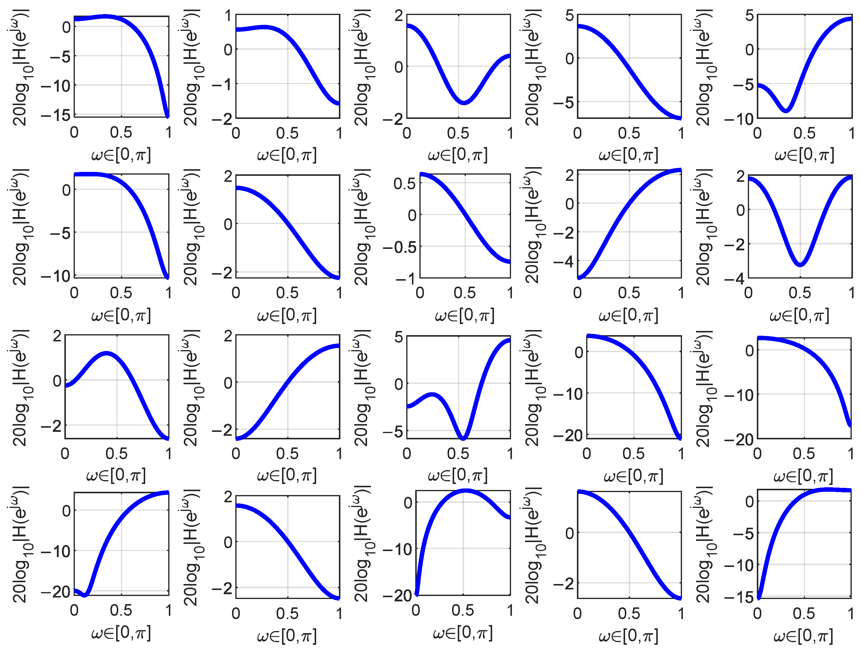
The magnitude responses of the learned filters in the Corn moisture analysis using FPLS are shown in Figure 5. The maximum number of components is 20, resulting in 20 deflation processes. Each time a deflation process is completed, a new filter is learned. Consequently, a total of 20 filters are obtained. For simplicity, only the filters learned from the deflation processes that resulted in the minimum RMSEP for moisture prediction are depicted in Figure 5. From this figure, it can be observed that one of the learned filter may be a low-pass, high-pass, band-pass, or band-stop filter. The characteristics of the filter are obtained based on the training samples. In subsequent experiments, for the sake of simplicity, we will no longer present the magnitude–frequency response of the learned filters.

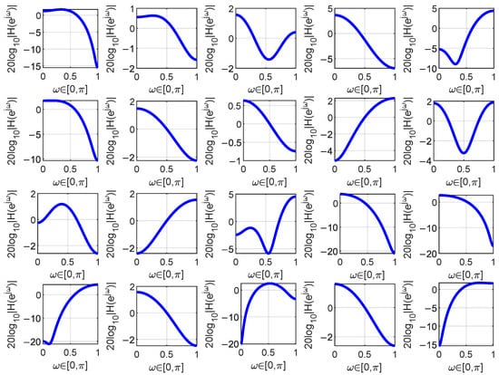
Figure 5. The filters learned during one iteration when analyzing the moisture content in the Corn dataset are depicted. The blue curve in the figure represents the magnitude frequency response of the filter.

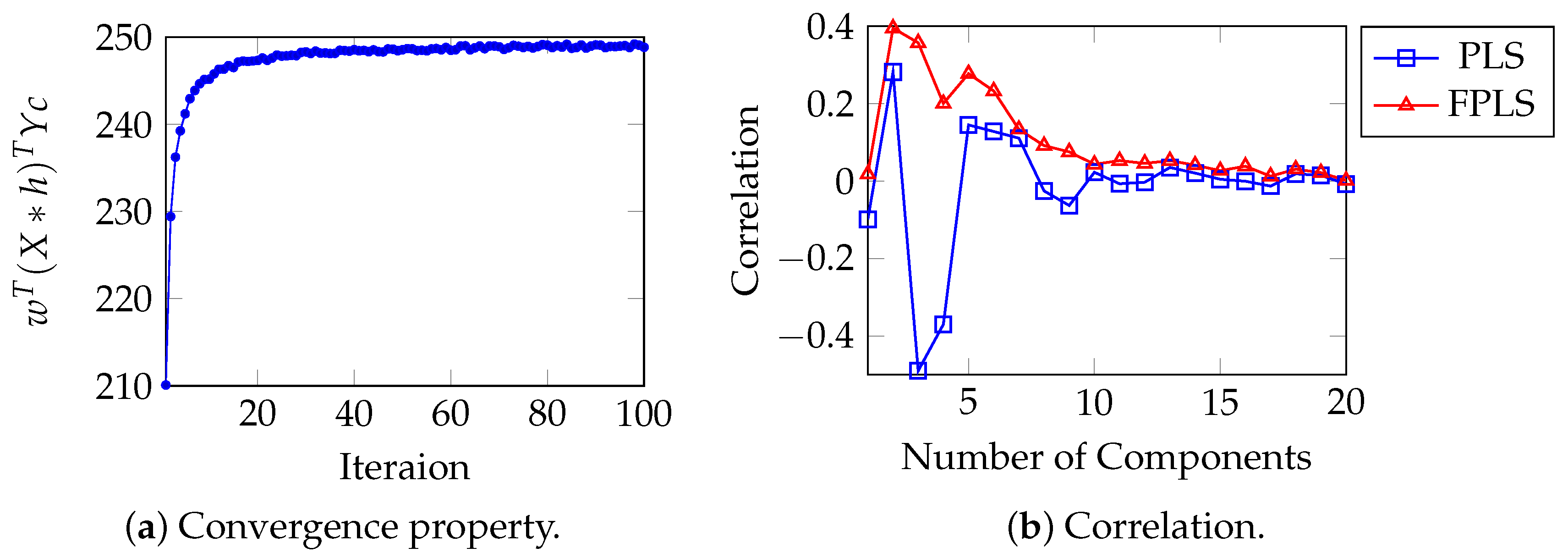
For moisture, oil, protein, and starch prediction, the initially learned filters for each target are $h_{moisture}=[-0.7164,-0.6611,0.2228]$, $h_{oil}=[0.2190,0.7080,0.6714]$, $h_{protein}=[-0.1730,-0.9849]$, and $h_{starch}=[-0.2478,0.0498,-0.9675]$. At this moment, ${\displaystyle \frac{w^T{(X\ast h_{moisture})}^{T}Y}{w^T{X}^{T}Y}}$$=1.3331<N=3$, ${\displaystyle \frac{w_i^T{(X\ast h_{oil})}^{T}Y}{w_j^T{X}^{T}Y}}=2.5484<3$, ${\displaystyle \frac{w_i^T{(X\ast h_{protein})}^{T}Y}{w_j^T{X}^{T}Y}}=1.3399<2$, and ${\displaystyle \frac{w_i^T{(X\ast h_{starch})}^{T}Y}{w_j^T{X}^{T}Y}}=1.3520<2$ are all consistent with our previous analysis in Section 3.3. The convergence behavior with respect to iteration numbers is presented in Figure 6, which simultaneously demonstrates the correlation between the projections of test samples from both PLS and FPLS models onto the weight vector w and their corresponding moisture content values.

Figure 6. (a) $w^T{(X\ast h)}^{T}Yc$ converges as iteration increases. (b) Correlation between the projection of the test samples of PLS, FPLS models on vector w, and the moisture content.

4.2. Octane Dataset Analysis

This dataset contains 39 near-infrared spectra, which need to be modeled to predict the content of Octane. The wavelength range is 1100–1550 nm with 2 nm intervals. The range of Octane is 86.7–92.4%. We use the original spectra from the dataset for modeling and analysis [31,32]. The best mean RMSEP values for FPLS, PLS, OSCPLS, VCPLS, PoPLS, LoPLS, DOSC, OPLS, MSC, SNV, SGFilter, and Lasso are listed in Table 3. The numbers in parentheses indicate the number of components. Table 3 also presents the upper and lower bounds of RMSEP, as well as the lower bound of CS.

Table 3. Quantitative analysis results in terms of RMSEP, prediction variance, Lower and Upper boundaries of RMSEP and lower boundary of CS. The proposed FPLS is compared to PLS, OSCPLS, VCPLS, PoPLS, LoPLS, DOSC, OPLS, MSC, SNV, SGFilter, and Lasso using the Octane dataset.

Method	Octane
	RMSEP	Variance	CS	Lower RMSEP	Upper RMSEP	Lower CS
FPLS	0.0645 (16)	0.0165	0.9998	0.0015	2.7065	0.9994
PLS	0.0949 (3)	0.0166	0.9911	0.0796	2.2716	0.9894
OSCPLS	0.0883 (2)	0.0045	0.9910	0.0766	2.2711	0.9898
VCPLS	0.4435 (9)	0.0413	0.9798	0.4752	2.4115	0.9736
PoPLS	0.3036 (3)	0.0296	0.9477	0.4735	2.8059	0.9352
LoPLS	0.0950 (3)	0.0167	0.9899	0.0811	2.7219	0.9892
DOSC	0.0885 (2)	0.0043	0.9990	0.0766	2.2711	0.9898
OPLS	0.0949 (2)	0.0049	0.9988	0.0766	2.2711	0.9898
MSC	0.0843 (2)	0.0049	0.9995	0.0038	2.7065	0.9991
SNV	0.0945 (2)	0.0049	0.9994	0.0045	2.7065	0.9988
SGFilter	0.0853 (2)	0.0049	0.9990	0.0796	2.2716	0.9894
Lasso	0.4313 (1)	0.0354	0.9894	0.0796	2.2716	0.9750

Based on the RMSEP and variance values presented in Table 3, we found that FPLS stands out with the lowest RMSEP value of 0.0645, indicating its exceptional predictive accuracy. The moderate variance suggests stability in its predictions, despite the relatively high number of components (15). PLS follows closely with a competitive RMSEP and variance, making it a viable alternative. OSCPLS and VCPLS, while offering comparable RMSEP values, exhibit higher variance, potentially indicating less stability. On the other hand, methods like PoPLS and LoPLS offer lower variance but at a cost of higher RMSEP values, suggesting a trade-off between stability and accuracy. DOSC and OPLS present intermediate RMSEP values with moderate variance, balancing both aspects. MSC, SNV, and SGFilter, despite their simplicity, demonstrate competitive RMSEP values with varying degrees of variance. Lasso, with its significantly higher RMSEP and moderate variance, may not be the optimal choice for predictive accuracy. The number of components for each method also plays a role, as more components can potentially increase complexity and computational cost. The boundaries of RMSEP and CS are consistent with Equations (33) and (37).

Figure 7 shows that the mean RMSEP of Octane prediction varies with an increasing number of components. Among these methods, FPLS exhibits a faster decline in RMSEP compared to other approaches. Furthermore, beyond a certain number of components, the RMSEP of FPLS becomes significantly smaller than that of other methods. Specifically, the number of components is observed to be 3 for Octane prediction. This figure also validates the effectiveness of the proposed FPLS model.

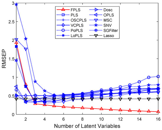
Figure 7. RMSEP values of Octane prediction using FPLS, PLS, OSCPLS, VCPLS, PoPLS, LoPLS, DOSC, OPLS, MSC, SNV, and SGFilter models with 1–16 components. Lasso is different from the previous methods. It is a feature selection method. The horizontal axis in the RMSEP graph represents the number of random experiments for Lasso.

Prediction variance of FPLS is essentially consistent with that of PLS, which is consistent with our analysis in Section 3.3. For the first filter learned for FPLS, $h_{octane}=[-0.0765,-0.1345,-0.9879]$; thus, ${\displaystyle \frac{w^T{(X\ast h_{octane})}^{T}Y}{w^T{X}^{T}Y}}=71.1576/50.4151=1.4114<3$, which is consistent with our previous analysis.

4.3. Mango Dataset

This dataset contains 58 near-infrared spectroscopic data, which are used to develop prediction models to determine vitamin C (VC) and total acidity (TA) of intact mango fruits (https://data.mendeley.com/datasets/ph57ynng46/1 (accessed on 11 November 2023)). The range of the parameter are as follows: VC (189.72–772.77) and TA (28.93–35.66). The figures indicate milligrams per 100 g of fresh mass. The best RMSEP and prediction variance of FPLS, PLS, OSCPLS, VCPLS, PoPLS, LoPLS, DOSC, OPLS, MSC, SNV, SGFilter, and Lasso are listed in Table 4. Meanwhile, this table also provides the boundaries for RMSEP and CS.

Table 4. Quantitative analysis results in terms of RMSEP and RMSEP bounds. The proposed FPLS compared to PLS, OSCPLS, VCPLS, PoPLS, LoPLS DOSC, OPLS, MSC, SNV, SGFilter, and Lasso using the Mango dataset.

Method	Total Acidity				Vitamin C
	RMSEP	Variance	Lower RMSEP	Upper RMSEP	RMSEP	Variance	Lower RMSEP	Upper RMSEP
FPLS	0.2731 (10)	0.0191	0.2310	1.7415	0.6988 (10)	0.0196	0.5006	2.1907
PLS	0.4328 (5)	0.0239	0.3696	1.8053	1.1015 (5)	0.0248	0.9996	2.4569
OSCPLS	0.4837 (2)	0.0004	0.3832	1.8122	1.2581 (3)	0.0753	0.9129	2.3978
VCPLS	0.4912 (8)	0.0043	0.3248	1.7831	1.3499 (1)	0.1033	1.1249	2.5569
PoPLS	0.4396 (10)	0.0081	0.4225	1.8334	1.1491 (4)	0.0141	1.2111	2.6385
LoPLS	0.4332 (5)	0.0239	0.4222	1.8333	1.1023 (5)	0.0248	1.0504	2.4951
DOSC	0.4818 (2)	0.0025	0.3832	1.8122	1.2568 (3)	0.0743	0.9129	2.3978
OPLS	0.4433 (4)	0.0013	0.3615	1.8011	1.0847 (4)	0.0167	1.0376	2.4852
MSC	0.3825 (6)	0.0014	0.3841	1.6631	1.0797 (6)	0.0192	0.5573	2.2137
SNV	0.3829 (6)	0.0014	0.3844	1.6632	1.0820 (6)	0.0194	0.5573	2.2137
SGFilter	0.4201 (5)	0.0014	0.3696	1.8053	1.0969 (7)	0.0186	1.0002	2.4573
Lasso	0.5035 (1)	0.0074	0.3696	1.8053	1.2863 (1)	0.0488	1.0002	2.4573

Based on the RMSEP and variance data presented in Table 4, in TA prediction, FPLS exhibits the lowest RMSEP value of 0.2731 with a variance of 0.0191, suggesting excellent predictive performance and stability. The relatively high number of components (10) may have contributed to its accuracy. On the other hand, models like OSCPLS, VCPLS, DOSC, and Lasso have higher RMSEP values, indicating poorer predictive accuracy. For instance, Lasso has the highest RMSEP of 0.5035 with a variance of 0.0074, despite using only 1 component. This suggests that the model may be overfitting or not capturing the underlying patterns in the data well. Models such as PLS, PoPLS, LoPLS, OPLS, MSC, SNV, and SGFilter lie somewhere in the middle, with RMSEP values ranging from 0.3825 to 0.4433. Their variances are also relatively low, indicating that these models are somewhat stable in their predictions. The number of components used in these models varies, suggesting that the optimal number of components may depend on the specific characteristics of the data and the model. FPLS stands out as the top-performing model in TA prediction, while Lasso needs further improvement to achieve better predictive accuracy.

In VC prediction, FPLS also exhibits a relatively low RMSEP value of 0.6988 with a variance of 0.0196, suggesting good predictive performance and stability. The use of 10 components may have contributed to its ability to capture more of the underlying patterns in the data. Models like OSCPLS, VCPLS, and Lasso have higher RMSEP values, indicating poorer predictive accuracy. For instance, Lasso has the highest RMSEP of 1.2863 with a variance of 0.0488, which may be due to its use of only 1 component, limiting its ability to model complex patterns. Models such as PLS, PoPLS, LoPLS, OPLS, MSC, SNV, and SGFilter lie somewhere in the middle, with RMSEP values ranging from around 1.08 to 1.10. Their variances are also relatively low, indicating that these models are somewhat stable in their predictions. The number of components used in these models varies, suggesting that the optimal number may depend on the specific characteristics of the data and the problem being addressed.

Figure 8a,b show mean RMSEP for the TA and VC varying with the increasing number of components, respectively. Among these methods, FPLS exhibits a faster decline in RMSEP compared to other approaches. Furthermore, beyond a certain number of components, the RMSEP of FPLS becomes significantly smaller than that of other methods. Specifically, the number of components is observed to be 4 for TA prediction and 3 for VC. These figures also validate the effectiveness of the FPLS method.

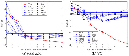
Figure 8. RMSEP values of the TA and VC prediction using FPLS, PLS, OSCPLS, VCPLS, PoPLS, LoPLS, DOSC, OPLS, MSC, SNV, and SGFilter models with 1–10 components. Lasso is different from the previous methods. It is a feature selection method. The horizontal axis in the figure represents the number of random experiments for Lasso.

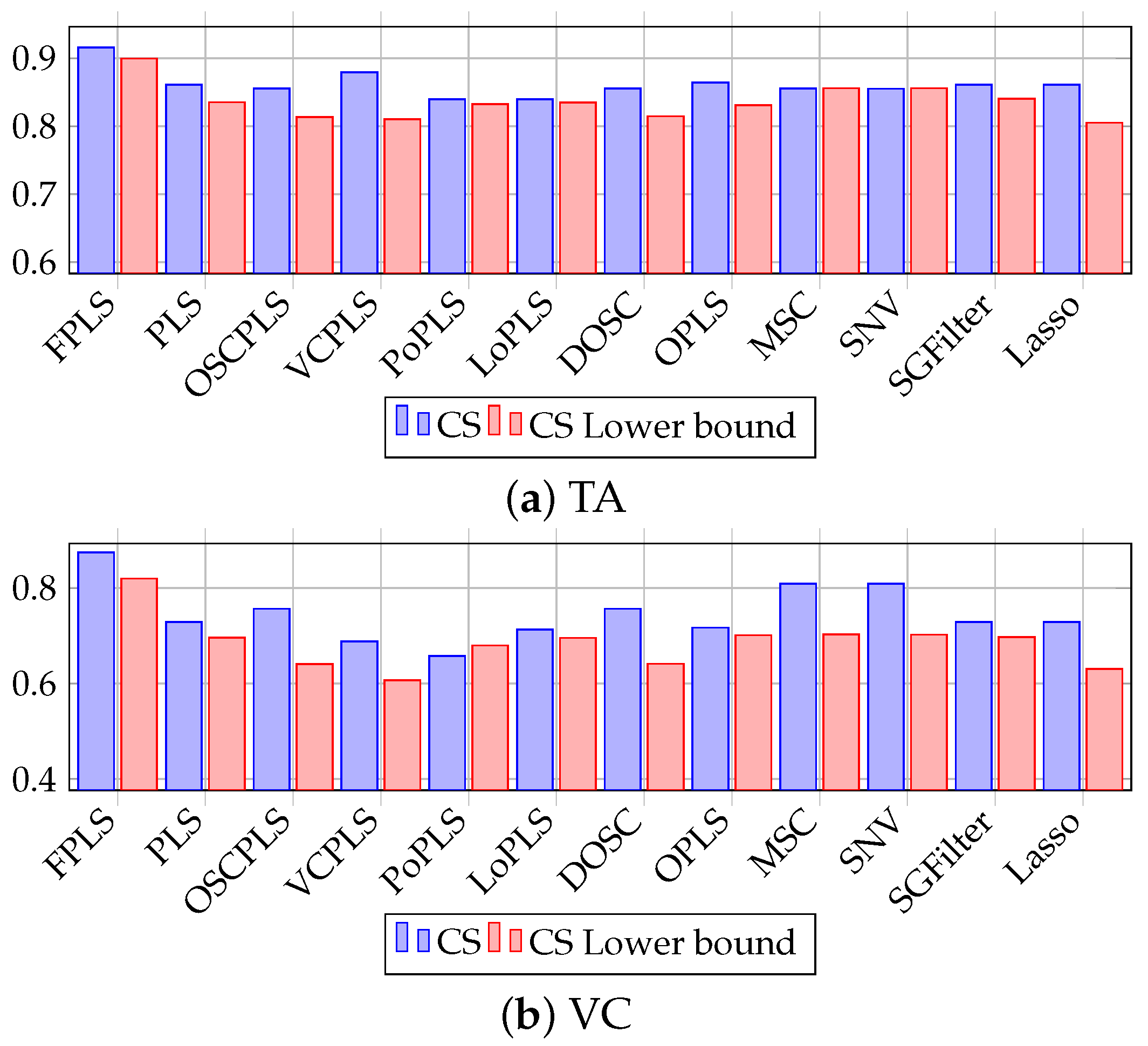
Figure 9 depicts the CS plot of the predicted values for TA and VC. The data in the figure indicate that CS and its lower bound satisfy Equation (33). Considering the correlation between prediction and target, it is evident that the FPLS model proposed in this paper yields the best predictive results.

Figure 9. CS plot of TA and VC prediction using FPLS, PLS, OSCPLS, VCPLS, PoPLS, LoPLS, DOSC, OPLS, MSC, SNV, SGFilter, and Lasso. The horizontal axis represents methods, while the vertical axis represents CS and its lower bound.

According to Table 4 and Figure 8 and Figure 9, the proposed FPLS outperforms PLS, OSCPLS, VCPLS, PoPLS, LoPLS, DOSC, OPLS, MSC, SNV, SGFilter, and Lasso in terms of RMSEP for TA and VC prediction. The first filters learned for Mango TA and VC analysis are $h_{TA}=[-0.0630,0.5889,0.8057]$ and $h_{VC}=[-0.4626,-0.8547,-0.2355]$; thus, ${\displaystyle \frac{w^T{(X\ast h_{TA})}^{T}Y}{w^T{X}^{T}Y}}=1.7297<3$ and ${\displaystyle \frac{w^T{(X\ast h_{VC})}^{T}Y}{w^T{X}^{T}Y}}=2.4060<3$, which are consistent with our previous analysis.

4.4. Soil Available Nitrogen Dataset

At the Yesheng Gongmi planting base in Wuzhong City, Ningxia, 75 soil samples were collected from plot 2 (954 mu, 1 mu ≈ 0.1647 acres) (https://www.scidb.cn/en/detail?dataSetId=93899ccb63054b5fb663c010d88892c8&version=V1 (accessed on 2 December 2023)). After removing impurities, the collected soil samples were allowed to air-dry naturally. The dried soil samples were then manually ground and sieved using a 60-mesh sieve, according to the requirements of the analysis project. The soil samples were sealed in self-sealing bags and uniformly numbered [33]. This experiment aims to predict the Soil Available Nitrogen content, which ranges from 39.48 to 86.73 (mg/kg).

The best mean RMSEP and corresponding prediction variances of FPLS, PLS, OSCPLS, VCPLS, PoPLS, LoPLS, DOSC, OPLS, MSC, SNV, SGFilter, and Lasso are listed in Table 5. The figure in parentheses indicates the corresponding number of components when the RMSEP reaches its minimum value.

Table 5. Quantitative analysis results in terms of prediction variance, RMSEP—including its lower and upper bounds—as well as CS and its lower bound. The proposed FPLS is compared to PLS, OSCPLS, VCPLS, PoPLS, LoPLS, DOSC, OPLS, MSC, SNV, SGFilter, and Lasso using the Soil Available Nitrogen dataset.

Method	Nitrogen
	RMSEP	Variance	CS	Lower RMSEP	Upper RMSEP	Lower CS
FPLS	4.2388 (18)	0.5872	0.9667	2.8807	9.5146	0.9506
PLS	6.0781 (7)	0.7593	0.9561	3.7772	9.5697	0.9283
OSCPLS	7.4131 (1)	1.0854	0.9356	5.4830	9.6807	0.9118
VCPLS	8.0386 (1)	0.9987	0.9364	5.4172	9.6763	0.9040
PoPLS	6.4054 (5)	0.7488	0.9410	5.0373	9.6509	0.9243
LoPLS	5.9168 (6)	0.7523	0.9427	4.8964	9.6416	0.9303
DOLS	7.4078 (1)	1.0842	0.9306	5.8935	9.7087	0.9119
OPLS	6.0622 (6)	1.2427	0.9330	5.6967	9.6953	0.9285
MSC	6.1594 (7)	0.6804	0.9331	5.6885	9.6947	0.9273
SNV	6.1596 (7)	0.6798	0.9331	5.6885	9.6947	0.9273
SGFilter	6.0766 (7)	0.7792	0.9212	6.6591	9.7624	0.9284
Lasso	8.6914 (1)	1.5812	0.9212	6.6591	9.7624	0.8958

According to Table 5, FPLS exhibits a relatively low RMSEP value of 4.2388 with a variance of 0.5872, suggesting good predictive performance and stability. The use of 18 components may have contributed to its ability to capture more of the underlying patterns in the data. On the other hand, models like OSCPLS, VCPLS, DOLS, and Lasso have higher RMSEP values, indicating poorer predictive accuracy. For instance, Lasso has the highest RMSEP of 8.6914 with a variance of 1.5812, which may be due to its use of only 1 component, limiting its ability to model complex patterns in the data. Models such as PLS, PoPLS, LoPLS, OPLS, MSC, SNV, and SGFilter lie somewhere in the middle, with RMSEP values ranging from around 6.06 to 6.16. Their variances are also relatively low, indicating that these models are somewhat stable in their predictions. The number of components used in these models varies, suggesting that the optimal number may depend on the specific characteristics of the data and the problem being addressed. This table also provides the boundaries of RMSEP and CS, which are consistent with our analysis at the beginning of Section 2.

Figure 10 shows the nitrogen mean RMSEP varying with the number of components. Among these methods, FPLS exhibits a faster decline in RMSEP compared to other approaches. Furthermore, beyond a certain number of components, the RMSEP of FPLS becomes significantly smaller than that of other methods. Specifically, for FPLS, the optimal number of components is observed to be 6. The curves in this figure also validate the effectiveness of the FPLS method in achieving accurate soil nitrogen predictions.

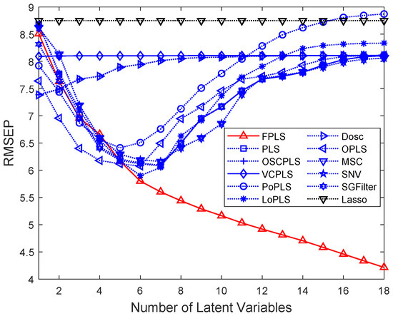
Figure 10. RMSEP values of the prediction using FPLS, PLS, OSCPLS, VCPLS, PoPLS, LoPLS, DOSC, OPLS, MSC, SNV, and SGFilter models with 1–18 components. Lasso is different from the previous methods. It is a feature selection method. The horizontal axis in the figure represents the number of random experiments for Lasso.

According to Table 5 and Figure 10, the proposed FPLS outperforms PLS, OSCPLS, VCPLS, PoPLS, LoPLS, DOSC, OPLS, MSC, SNV, SGFilter, and Lasso on nitrogen prediction in terms of RMSEP. The first filter learned for soil nitrogen concentration prediction is $h_{nitr}=[-0.5452,0.1408,-0.7170,-0.4110]$; thus, ${\displaystyle \frac{w^T{(X\ast h_{nitr})}^{T}Y}{w^T{X}^{T}Y}}=2.3275<4$, which is consistent with our analysis in Section 3.3.

To verify the robustness of the algorithm, we added 0.01 watts of Gaussian noise to both the training and testing datasets before constructing the models for analysis. The results are shown in Figure 11.

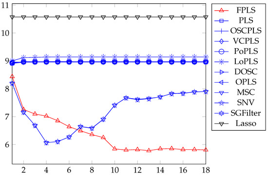
Figure 11. Experimental results with noise.

5. Conclusions

This study proposes a new Partial Least Squares regression model, FPLS. This model integrates filter learning and traditional PLS models into a single model. It can adaptively learn the parameters of the filter and PLS, improving the effectiveness of the filter. At the same time, we briefly analyze the convergence of the model, the bounds of the objective function, and the variance of the prediction distribution. Experiments on four datasets, Corn, Octane, Mango and Soil, verify the effectiveness, convergence, and bounds of the objective function of the model. Future work will primarily encompass the following aspects:

• Further exploration of the relationship between filter length and ${\displaystyle \frac{w^T{(X\ast h)}^{T}Yc}{w^T{X}^{T}Yc}}$. In Figure 2, we pointed out its connection with local smoothness, and consequently chose filter lengths of 2, 3, and 4. Actually, as the length increases, ${\displaystyle \frac{w^T{(X\ast h)}^{T}Yc}{w^T{X}^{T}Yc}}$ exhibits a distinct regularity as shown in Figure 12a. Further in-depth research will be conducted on this issue.
  

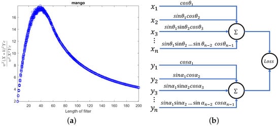  Figure 12. Issues that require further research. (a) Relationship between ${\displaystyle \frac{w^T{(X\ast h)}^{T}Yc}{w^T{X}^{T}Yc}}$ and filter length; (b) a potential network structure.
• Utilizing trigonometric functions to transform the constraint condition ${\parallel w\parallel }_2=1$. Define $w_1=cos{\theta }_1$, $w_2=sin{\theta }_{1}cos{\theta }_2$, $w_3=sin{\theta }_{1}sin{\theta }_{2}cos{\theta }_3,\cdots ,w_{n-1}=sin{\theta }_{1}sin{\theta }_2\cdots sin{\theta }_{n-2}cos{\theta }_{n-1}$, $w_n=sin{\theta }_{1}sin{\theta }_2\cdots$$sin{\theta }_{n-2}sin{\theta }_{n-1}$. In this way, we obtain a framework that utilizes neural networks to compute with orthogonal constraints, as shown in Figure 12b. Whether this network is equivalent to the BP network with 2-norm constraint requires further research.
• Utilizing a dilated filter to achieve multi-scale feature extraction. The filter can be generalized to $h=\left[h_1,\underset{m}{\underbrace{0,\cdots ,0}},h_2,\underset{m}{\underbrace{0,\cdots ,0}},\cdots ,h_n\right]$. What is the relationship between this network and existing neural networks? This is an open question.

References

- Wold, S.; Sjöström, M.; Eriksson, L. PLS-regression: A basic tool of chemometrics. Chemom. Intell. Lab. Syst. 2001, 58, 109–130. [Google Scholar] [CrossRef]
- Roy, I.G. On computing first and second order derivative spectra. J. Comput. Phys. 2015, 295, 307–321. [Google Scholar] [CrossRef]
- Zhang, X.D. Modern Signal Processing; Walter de Gruyter GmbH & Co KG: Berlin, Germany, 2022. [Google Scholar] [CrossRef]
- Wold, S.; Trygg, J.; Berglund, A.; Antti, H. Some recent developments in PLS modeling. Chemom. Intell. Lab. Syst. 2001, 58, 131–150. [Google Scholar] [CrossRef]
- Wold, S.; Kettaneh-Wold, N.; Skagerberg, B. Nonlinear PLS modeling. Chemom. Intell. Lab. Syst. 1989, 7, 53–65. [Google Scholar] [CrossRef]
- Krishnan, A.; Williams, L.J.; McIntosh, A.R.; Abdi, H. Partial Least Squares (PLS) methods for neuroimaging: A tutorial and review. Neuroimage 2011, 56, 455–475. [Google Scholar] [CrossRef]
- Lindgren, F.; Geladi, P.; Wold, S. The kernel algorithm for PLS. J. Chemom. 1993, 7, 45–59. [Google Scholar] [CrossRef]
- De Jong, S.; Ter Braak, C.J. Comments on the PLS kernel algorithm. J. Chemom. 1994, 8, 169–174. [Google Scholar] [CrossRef]
- De Jong, S. SIMPLS: An alternative approach to partial least squares regression. Chemom. Intell. Lab. Syst. 1993, 18, 251–263. [Google Scholar] [CrossRef]
- Rännar, S.; Lindgren, F.; Geladi, P.; Wold, S. A PLS kernel algorithm for data sets with many variables and fewer objects. Part 1: Theory and algorithm. J. Chemom. 1994, 8, 111–125. [Google Scholar] [CrossRef]
- Andersson, M. A comparison of nine PLS1 algorithms. J. Chemom. 2009, 23, 518–529. [Google Scholar] [CrossRef]
- Sæbø, S.; Almøy, T.; Flatberg, A.; Aastveit, A.H.; Martens, H. LPLS-regression: A method for prediction and classification under the influence of background information on predictor variables. Chemom. Intell. Lab. Syst. 2008, 91, 121–132. [Google Scholar] [CrossRef]
- Wold, S.; Antti, H.; Lindgren, F.; Öhman, J. Orthogonal signal correction of near-infrared spectra. Chemom. Intell. Lab. Syst. 1998, 44, 175–185. [Google Scholar] [CrossRef]
- Trygg, J.; Wold, S. Orthogonal projections to latent structures (O-PLS). J. Chemom. 2002, 16, 119–128. [Google Scholar]
- Westerhuis, J.A.; De Jong, S.; Smilde, A.K. Direct orthogonal signal correction. Chemom. Intell. Lab. Syst. 2001, 56, 13–25. [Google Scholar] [CrossRef]
- Geladi, P.D.; Macdougall, D.B.; Martens, H. Linearization and Scatter-Correction for Near-Infrared Reflectance Spectra of Meat. Appl. Spectrosc. 1985, 39, 491–500. [Google Scholar] [CrossRef]
- Barnes, R.J.; Dhanoa, M.S.; Lister, S.J. Standard Normal Variate Transformation and De-trending of Near-Infrared Diffuse Reflectance Spectra. Appl. Spectrosc. 1989, 43, 772–777. [Google Scholar] [CrossRef]
- Rinnan, A.; Berg, V.F.; Engelsen, S.B. Review of the most common pre-processing techniques for near-infrared spectra. Trend. Anal. Chem. 2009, 28, 1201–1222. [Google Scholar] [CrossRef]
- Li, S.; Nyagilo, J.O.; Dave, D.P.; Wang, W.; Zhang, B.; Gao, J. Probabilistic partial least squares regression for quantitative analysis of Raman spectra. Int. J. Data Min. Bioinform. 2015, 11, 223–243. [Google Scholar] [CrossRef]
- Yang, X.; Liu, X.; Xu, C. Robust Mixture Probabilistic Partial Least Squares Model for Soft Sensing With Multivariate Laplace Distribution. IEEE Trans. Instrum. Meas. 2020, 70, 3000109. [Google Scholar] [CrossRef]
- Rosipal, R.; Trejo, L.J. Kernel Partial Least Squares Regression in Reproducing Kernel Hilbert Space. J. Mach. Learn. Res. 2002, 2, 97–123. [Google Scholar]
- Chen, H.; Sun, Y.; Gao, J.; Hu, Y.; Yin, B. Solving Partial Least Squares Regression via Manifold Optimization Approaches. IEEE Trans. Neural Netw. Learn. Syst. 2019, 30, 588–600. [Google Scholar] [CrossRef]
- Xie, Z.; Feng, X.; Chen, X. Partial least trimmed squares regression. Chemom. Intell. Lab. Syst. 2022, 221, 104486. [Google Scholar] [CrossRef]
- Mohammadi, A.; Almasganj, F.; Taherkhani, A.; Naderkhani, F. Missing Feature reconstruction with Multivariate Laplace distribution (MLD) for noise robust phoneme recognition. In Proceedings of the 2008 3rd International Symposium on Communications, Control and Signal Processing, Saint Julian’s, Malta, 12–14 March 2008. [Google Scholar] [CrossRef]
- Boccard, J.; Rutledge, D.N. A consensus orthogonal partial least squares discriminant analysis (OPLS-DA) strategy for multiblock Omics data fusion. Anal. Chim. Acta 2013, 769, 30–39. [Google Scholar] [CrossRef] [PubMed]
- Wang, H. Partial Least-Squares Regression Method and Applications; National Defense Industry Press: Beijing, China, 1999; pp. 152–153. [Google Scholar]
- Höskuldsson, A. PLS regression methods. J. Chemom. 1988, 2, 211–228. [Google Scholar] [CrossRef]
- Jiang, X.; You, X.; Yu, S.; Tao, D.; Chen, C.P.; Cheung, Y.M. Variance constrained partial least squares. Chemom. Intell. Lab. Syst 2015, 145, 60–71. [Google Scholar] [CrossRef]
- Indahl, U. A twist to partial least squares regression. J. Chemom. 2005, 19, 32–44. [Google Scholar] [CrossRef]
- Tibshirani, R. Regression shrinkage and selection via the lasso. J. R. Stat. Soc. B 1996, 58, 267–288. [Google Scholar] [CrossRef]
- Lee, S.; Shin, H.; Billor, N. M-type smoothing spline estimators for principal functions. Comput. Stat. Data Anal. 2013, 66, 89–100. [Google Scholar] [CrossRef]
- Esbensen, K.H.; Guyot, D.; Westad, F.; Houmøller, L.P. Multivariate Data Analysis-In Practise: An Introduction to Multivariate Data Analysis and Experimental Design; Gtap Technical Papers; Wiley: Hoboken, NJ, USA, 2002. [Google Scholar] [CrossRef]
- Wang, L. Optimization for Vis/NIRS Prediction Model of Soil Available Nitrogen Content. Chin. J. Lumin. 2018, 39, 1016–1023. [Google Scholar] [CrossRef]
Disclaimer/Publisher’s Note: The statements, opinions and data contained in all publications are solely those of the individual author(s) and contributor(s) and not of MDPI and/or the editor(s). MDPI and/or the editor(s) disclaim responsibility for any injury to people or property resulting from any ideas, methods, instructions or products referred to in the content. |
© 2025 by the authors. Licensee MDPI, Basel, Switzerland. This article is an open access article distributed under the terms and conditions of the Creative Commons Attribution (CC BY) license (https://creativecommons.org/licenses/by/4.0/).