Abstract
To ensure the product quality of a steel slab continuous casting machine, the mechanical alignment of the guide rolls must be monitored and corrected regularly. Misaligned guide rolls cause stress and strain in the partially solidified steel strand, leading to internal cracks and other quality issues. Current methods of alignment measurement are either not suited for regular maintenance or provide only indirect alignment information in the form of angle measurements. This paper presents three new algorithms that convert the available angle measurements into the absolute position of each guide roll, which is equivalent to the mechanical alignment. The algorithms are based on geometry and trigonometry or the gradient descent optimization algorithm. Under near ideal conditions, all algorithms yield very accurate position results. However, when tested and evaluated under various conditions, their susceptibility to real-world disturbances is revealed. Here, only the optimization-based algorithm reaches the desired accuracy. Under the influence of randomly distributed angle measurement errors with an amplitude of 0.01°, it is able to determine 90% of roll positions within mm of their actual position.
1. Introduction
In the past decades, continuous casting (CC) has evolved into the most important steel casting technology [1]. Today, about 96% of steel is produced worldwide using this complex process [2]. Due to this enormous throughput, increasing the reliability and efficiency of this process promises significant economical and ecological benefits. Reducing the amount of defects leads to less remelting and reworking, which is very costly in terms of time, material, machine and personnel usage [1]. Defects in the produced steel have a variety of causes, most commonly related to the chemical composition of the steel, the flow patterns, the cooling conditions in the mold and the secondary cooling zone as well as the mechanical condition of the casting machine [1,2,3,4,5,6,7].
This paper focuses on the latter point, more specifically on the alignment of the rolls that guide the strand on its way through the machine. The alignment describes how each roll position deviates from its position in the roll plan of the machine (see Figure 1). Usually, deviations between mm and mm are tolerated [8,9]. For the maintenance of caster segments in the factory workshop, the author of [10] even defines mm as their targeted tolerance. Such tight positioning tolerances are necessary because the partially solidified strand is in a very delicate state. Misaligned rolls exert excessive force on the strand, deforming it and causing mechanical strain within the material [11]. The solidification front within the strand is vulnerable to strains, ultimately leading to internal cracks [1,2,12,13,14,15,16,17]. Maintaining the best possible alignment of the guide rolls at all times is, therefore, a high priority for continuous casting machine (CCM) operators.
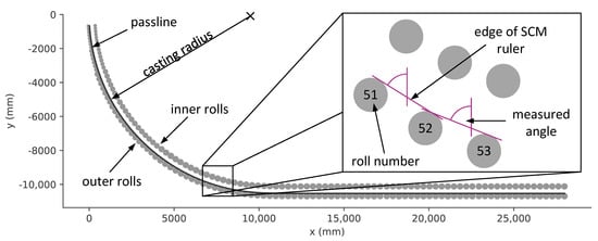
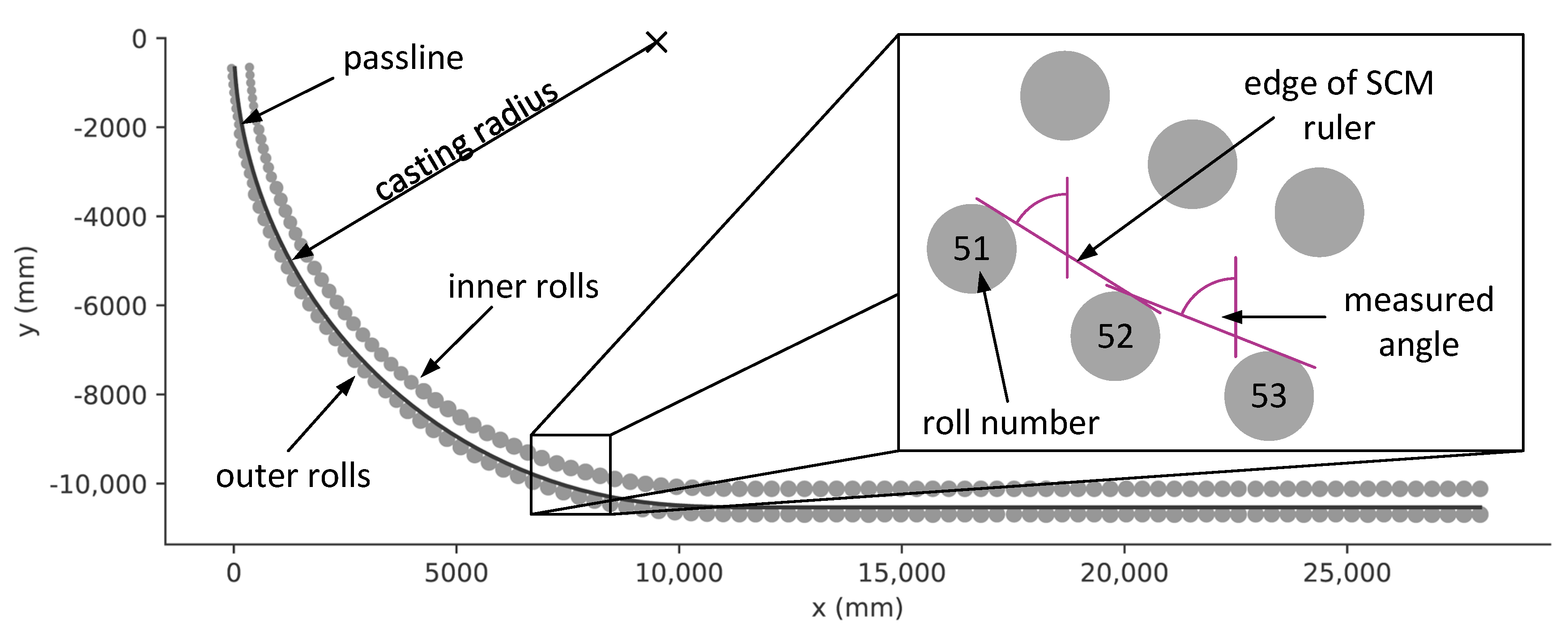
Figure 1.
Rollplan side view [18] and angle measurement principle. For clarity, the SCM itself is not shown. The “passline” is an imaginary line, which represents the contour of the strand backside under ideal alignment conditions. This line passes through the contact points between the outer rolls and the strands outer surface.
During casting, extreme forces and temperatures act on each roll, degrading their positional accuracies over time [2,14,19,20,21]. To maintain high-quality production at all times, the alignment must be checked and corrected regularly. However, measuring the alignment of a CCM within the desired accuracy is not a trivial task. The rough machine environment (dirt, cooling water, electromagnetic contamination, vibrations, etc.) and tight production schedules make measuring the positions of the guide rolls with the required precision very challenging. Given the tolerated position deviations, the measuring accuracy should be at least mm.
Devices like high precision total stations or laser trackers are often used to determine the alignment of CCM [8,10,20,22,23]. They are able to achieve the desired accuracy, which is why they are the standard in factory workshops where segments of the CCM are maintained, realigned and repaired. For regular in situ alignment measurements, however, these devices are unsuitable. They require long production pauses as well as trained and experienced personnel. In situ measurements are of crucial importance to CCM operators, since they provide information about which segments need to be replaced and how to realign the machine without time-intensive removal of segments.
The most common tool to measure the alignment in situ is a Strand Condition Monitoring System (SCM). SCMs are measuring systems that are integrated into the dummy bar of a CCM, which allows them to be pulled through the machine and physically touch and measure every roll. An SCM is fitted with spring-loaded rulers that push against and glide over the outer rolls, while the SCM travels through the casting machine. Each time a ruler has contact with two consecutive outer rolls, its angle is uniquely defined by the positions of the two rolls (see Figure 1). The rulers edge forms a tangent with the circumferences of the two rolls. This tangential angle is stored for each consecutive roll pair. The result of one measurement is, therefore, a set of angles, where n is the number of outer rolls. In this paper, a CCM with outer rolls is used as an example.
However, the tangential angles provided by an SCM are not immediately useful to a CCM operator [24]. To determine the impact of the rolls on the strand, their absolute positions with respect to the machines coordinate system must be known. Therefore, the angles must be converted into the x-y-positions of the rolls. Since the angle measurement is conducted in a rough environment, measurement errors are not entirely avoidable. Thus, the conversion from angles to positions must be as robust as possible against errors within the angle measurements. Developing and evaluating algorithms that robustly and precisely convert the set of angle measurements into n roll positions represents the contribution of this work.
In related work, some researchers have approached this problem. However, none of them aimed to compute all the roll positions in the global coordinate system of the CCM. Rather they usually only consider three consecutive rolls at a time. Sotnikov et al. [9] compute the “local radius” or “local curvature” using three consecutive rolls and relate it to the “preset radius”. The local radius is then used to estimate stress inside the strand material. Tokuda [12] uses an SCM to determine the tangential angles as described above. Applying trigonometry on the two angles measured between three consecutive rolls, they calculate the position deviation of the middle roll. This approach assumes, however, that the two outer rolls are perefectly aligned. The position of the middle roll will only be calculated relative to the outer rolls and not to the global coordinate system. The authors of [25], a manufacturer of SCM, use the same approach. They argue that roll positions are “double-checked” because the relative position to the rear and front roll is considered. Because this resolves the problem of calculation error accumulation (which will be discussed in detail in Section 4), they consider this the best approach. While it does not suffer from the error accumulation, it introduces the aforementioned problem of only producing a relative position result. This paper presents a holistic solution to this challenge that results in absolute values for the roll positions while significantly reducing the effect of calculation error accumulation.
2. Assumptions and Considerations
2.1. Radial and Tangential Error Components
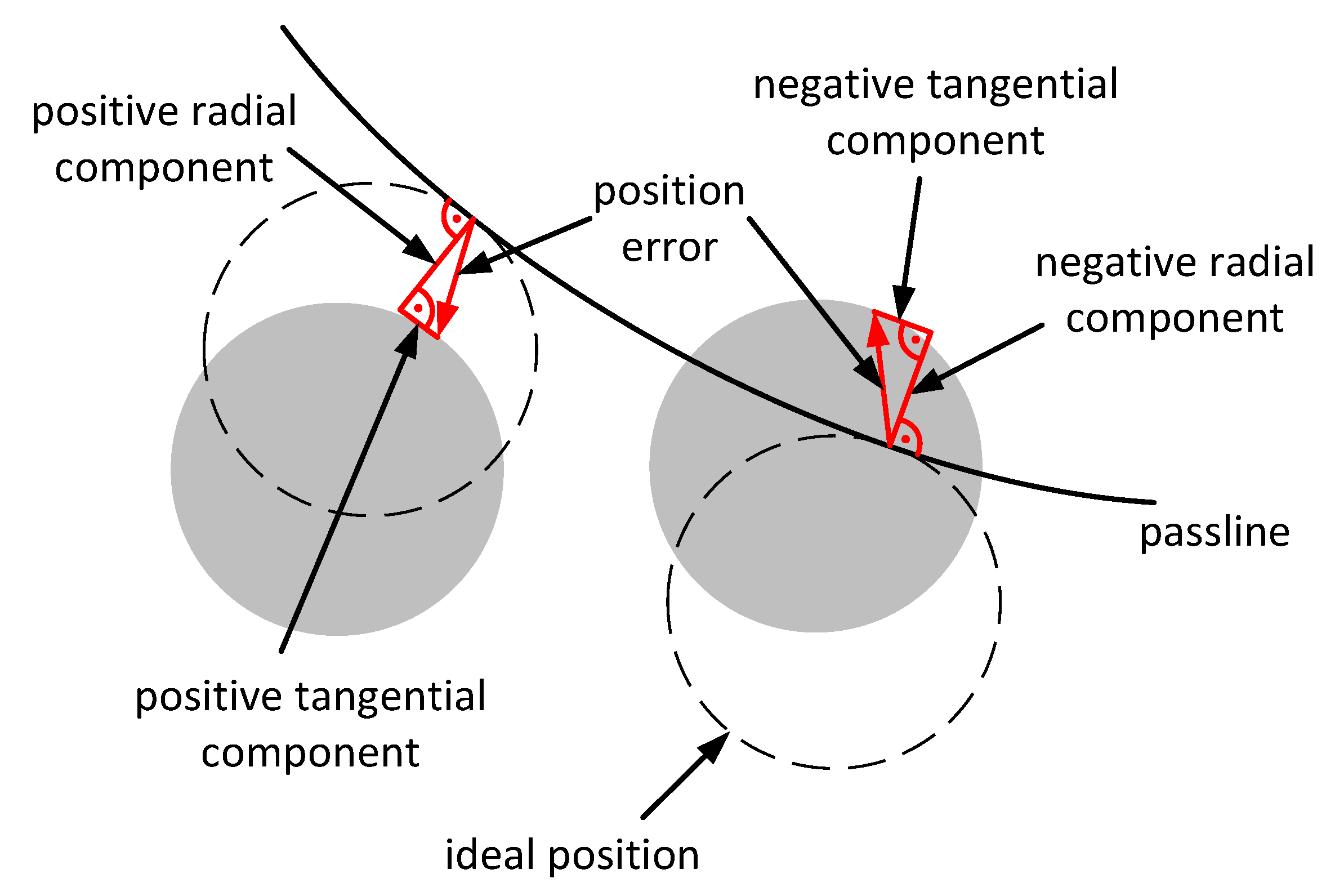
Roll position errors consist of two components: radial and tangential (see Figure 2). The radial component is perpendicular to the passline (see Figure 1), while the tangential component is tangential to the passline and thus always perpendicular to the radial component. The radial component gets its name from being colinear with the casting radius in the curved section of a CCM. In the horizontal section of the CCM, there is no casting radius, but the radial component is still defined as perpendicular to the passline. In this section of the machine, the passline is straight and has no tangent, so here, the tangential component is defined as parallel to the passline.
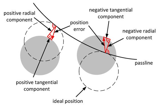
Figure 2.
Position error components and their directions. The component of the position error that is perpendicular to the passline is called “radial error” in reference to the CCMs casting radius (see Figure 1). The error component tangential to the passline is called “tangential”.
When a roll position deviates towards the outside of the casting arc (in the curved section) or towards the bottom of the machine (in the horizontal section), its radial error component is defined as positive. The positive direction for a tangential component is always in the direction of casting.
2.2. Indirect Relationship Between Angles and Positions
Figure 3 illustrates, why the measured angles are only an indirect measure of the alignment condition of a CCM. It shows four outer rolls with only radial error components (red), and the tangent lines (purple), whose angles an SCM would measure. A naive approach would directly compare the measured angles to the ideal angles defined by the roll plan. However, this approach will not be able to determine the errors of, for example, rolls 52 and 53 since the angle between them is consistent with the roll plan. On the other hand, looking at roll pair 54 and 55, the approach would report a difference between the measured and the ideal angle, even though roll 55 is in the correct position. Solving this issue is the main motivation for the development of the algorithms in this paper.
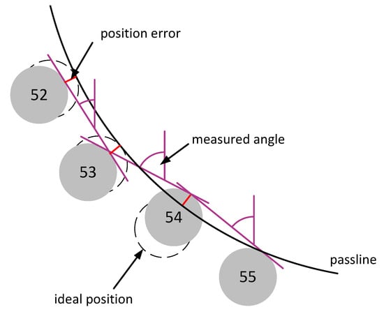
Figure 3.
Illustration of the indirect relationship between roll position errors and measured angles.
2.3. Solvability of the Problem
For the given mathematical problem to be solvable, the information provided by the SCM must be sufficient to determine the roll positions. The SCM provides angles, but the radial and tangential error components of each outer roll represent degrees of freedom. Two assumptions must be made to reduce the solution’s degrees of freedom:
- The first roll is in the perfect position.
- The tangential component of the deflection is zero.
The first assumption is necessary because the measured angles only provide a relative measurement, with no connection to the absolute coordinate system of the SCM. The known position of one roll provides an “anchor point” to the coordinate system. The first outer roll, often referred to as the “footroll”, is chosen and its position is assumed to always be ideal. Since it is the first roll to contact the strand, its influence on the quality is considerable. Thus, the position of this roll is monitored very strictly, making the assumption reasonable and reducing the degrees of freedom by 2.
The second assumption must be made because the measured tangents do not fully constrain the roll positions. Every roll could move in the direction of the tangent lines without changing the measured angle. This is a fundamental fact that cannot be overcome by an algorithm. Therefore, the assumption is made that each roll position error only contains a radial component. This reduces the degrees of freedom further by . Of course, in the real world, the roll errors do contain tangential components, which will cause the algorithms to produce systematic calculation errors. This will be investigated in detail in Section 4.
Under these assumptions, the degrees of freedom of the solution are reduced to
which is equal to the number of measured angles and thus leads to an unambiguously solvable system.
3. Angle Conversion Algorithms
In the following subsections, three different approaches are presented. They are named:
- Simplified Geometric.
- Full Geometric.
- Optimization-based.
The first two algorithms approach the problem purely geometrically. The simplified geometric approach makes additional assumptions about the machine geometry, which simplifies the equations. The full geometric approach considers every detail of the CCM’s geometry. The optimization-based approach uses an optimization algorithm with backpropagation and gradient descent to iteratively find an ideal solution.
However, before any of the algorithms is applied, a set of measured angles must be prepared using the so-called zero-mean compensation method.
3.1. Zero-Mean Compensation
This method compares the measured angles with the ideal angles, which are available from the CCM’s roll plan. The difference of each measured and ideal angle is calculated and all differences are averaged to yield
The angles and represent the measured and the ideal tangential angle between roll k and roll . The mean of the differences is then subtracted from every measured angle which sets the mean difference between the measured and ideal angles to zero. This method proved very effective in removing constant components from angle measurement errors, which can be detrimental to the performance of the algorithms. Its impact is analyzed in detail in Section 4.
3.2. Geometric Approaches
Both variants of the geometric approaches follow the same basic principle: Starting with the footroll, whose position is assumed to be ideal, a tangent line is laid against the circumference of the roll. The direction of this line is according to the measured angle between this roll and the following roll. Under the assumption that the position errors only contain radial components, the position of the following roll is calculated using trigonometric equations. The two variants of the geometric approaches use different sets of equations for this step.
Since the position of the second roll is now known, the process is repeated with the second and third roll, yielding the position of the third roll. This computational chain is repeated until the position of each roll is calculated.
The set of equations that are used by the simplified and the full geometric algorithm in each step are derived in the following subsections.
3.2.1. Simplified Geometric Approach
The simplified variant of the geometric approach makes additional assumptions about the CCMs geometry in order to simplify the calculation. These assumptions are:
- All rolls have the same diameter.
- The curvature of the circular section of the caster is negligibly small.
The geometry that emerges for two consecutive rolls under these additional assumptions is illustrated in Figure 4.

Figure 4.
Geometry of one step of the simplified geometric algorithm. Line is tangent to both rolls and represents the ruler’s edge. Due to the simplifying assumptions, the passline through is a straight line and both rolls have the same radius. This leads to the four right angles and the fact that the lines and are parallel.
The geometry leads to the the equations
and
Here, represents the measured angle. The points C and E mark the contact points of the rolls with the strand, if the roll’s positions were ideal. The line b is part of the passline, which is not curved due to the additional assumptions. Angle is the angle between line and a vertical line. This angle is independent from the roll’s positions and extracted from the roll plan. The angle is used to calculate the tangent inside the triangle BGF, which is combined with b to yield . This is added to the known radial error component of the first roll to finally yield the position error of the second roll.
The additional assumptions assure that the line is parallel to the tangent line , which represents the ruler’s edge. They also cause the triangle BGF to be right-angled. If these assumptions are not made and the curvature as well as the actual radii of the rolls are considered, the equations become much more complex, which is described in the following subsection.
3.2.2. Full Geometric Approach
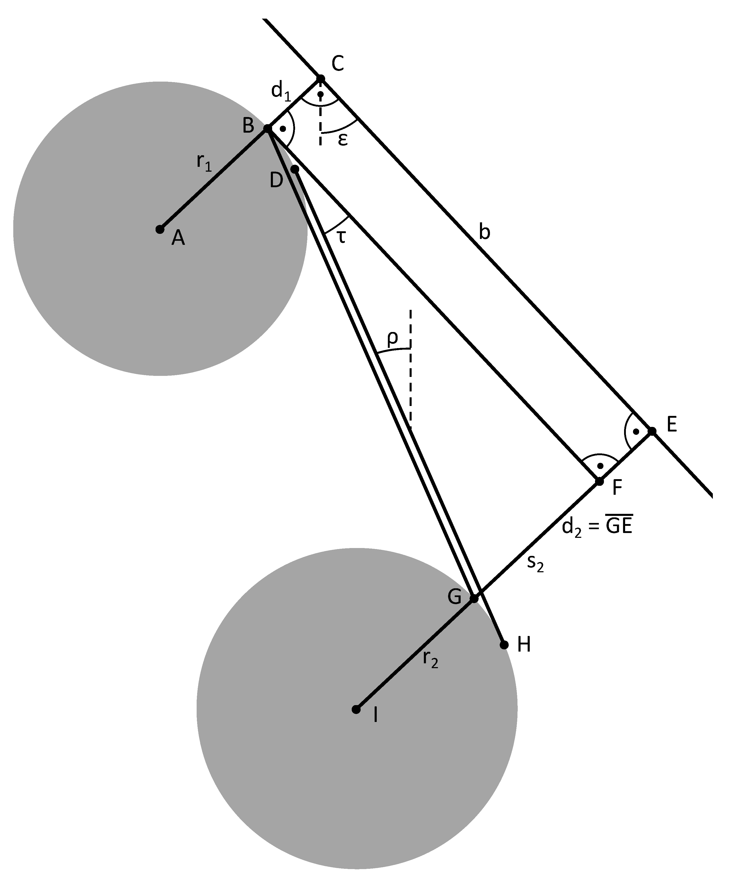
The full variant of the geometric approaches does not make additional assumptions about the machine geometry and, therefore, includes the casting radius and different roll radii in its equations. This approach results in two different cases with two slightly different sets of equations. Depending on the geometric circumstances at the current roll pair, the correct case has to be chosen before each step.
The underlying geometry of case 1 is shown in Figure 5. The line is tangent to both rolls and represents the rulers edge. Correspondingly, equals the measured angle. The distances and represent the radial components of the current and the next roll position error in the calculation chain. Similar to the simplified approach, the length b and the angle are independent from the roll positions and can be extracted from the roll plan. Note that b is a straight line, but the dashed passline is slightly curved. Also defined by the roll plan and independent of the roll positions are the angles and that are formed between a vertical line and a line through the roll’s center perpendicular to the passline. Through slightly different values for and , the machines curvature is considered. The values of and equal the radii of the two rolls. The angles formed by the radii with the tangent line are the only right angles in this diagram. The diagram shows the casting radius R, but it is not used in the equations.
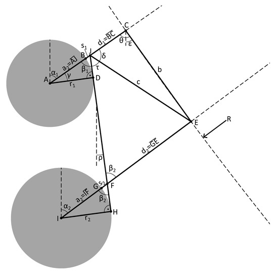
Figure 5.
Geometry of one step of the full geometric algorithm (case 1). The roll position errors in this figure are greatly exaggerated.
Mostly, case 1 and case 2 can be distinguished by the position of the short line segment . If is outside of the strand (to the left of the passline, when ), case 1 is used. If it is on the other side (), case 2 is used (see Figure 6). In the special case that intersects the passline, the sign of angle determines the case. These two special cases are not shown in dedicated figures. Table 1 summarizes the conditions under which each case is applied.
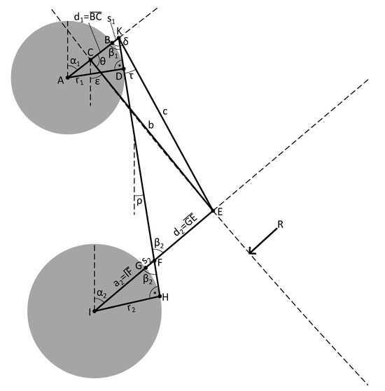
Figure 6.
Geometry of one step of the full geometric algorithm (case 2). The roll position errors in this figure are greatly exaggerated. The line is not shown for clarity.

Table 1.
Choices for the correct case of the full geometric approach.
With the two sets of equations that will be derived in the following paragraphs, every geometric case can be solved. Up to a point, however, the equations are identical for both cases. First, the angles
and
that are part of the right triangles are calculated using the measured angle . With the roll’s radii the lengths
and
are determined. Subsequently, the lengths of the short line sections
and
are calculated. The angle
needs to be determined, when in order to determine which case must be used.
Case 1.
In case 1, the angle
is calculated first. It is independent from the roll positions. Using and the cosine theorem, the length of line
is determined. Using c and a rearranged version of the cosine theorem, the angle
is calculated. In this step, division by zero when and are equal must be caught in code. In that case, . Finally, in case 1, the angle
is calculated. The last equation, which will yield , is the same in both cases and shown after the equations for case 2.
Case 2.
In case 2, whose geometry is illustrated in Figure 6, the equation for angle is
Note that in case 2, is on the other side of the passline. Next, using the cosine theorem in the triangle CKE, the length of
and the angle
are calculated, similarly to case 1. For , it holds that
The last equation is the same for both cases. It is based on the sine-theorem and yields
the radial component of the second roll’s position error.
The equations for one step of a geometric algorithm become significantly more complex when all aspects of the machine geometry are considered. The impact of the added complexity on the accuracy of the calculated roll position errors and the computational load will be discussed in Section 4.
3.3. Optimization-Based Approach
The geometric approaches calculate the positions of one roll at a time in a chain-like computation. As will be shown in Section 4, this works well as long as the measured angles are completely accurate. However, the geometric approaches can be sensitive to errors in the angle measurements. Since measurement errors are not avoidable in practice, this poses a significant challenge.
This leads to the idea to develop an algorithm that takes a different approach than the purely geometric ones. Rather than calculating the roll positions one-by-one, it should simultaneously consider all measured angles and compute all roll positions at once. With this in mind, an algorithm was developed that is based on the idea of optimization using backpropagation and gradient descent. It leverages the fact that the conversion of roll positions into tangential angles—the reverse of what the algorithm is supposed to calculate—is an easy and unambiguous trigonometric calculation that can be computed for all rolls at once. Rather than trying to directly convert the angles into the positions (as the geometric approaches do) the optimization-based algorithm systematically searches for a set of roll positions that would result in measured angles that are as close as possible to the actually measured angles. Optimization using gradient descent allows this to be performed without ever actually converting tangential angles into roll positions. The search is conducted in an iterative loop and each iteration of this loop consists of steps 3–7 of the following procedure (see Figure 7):
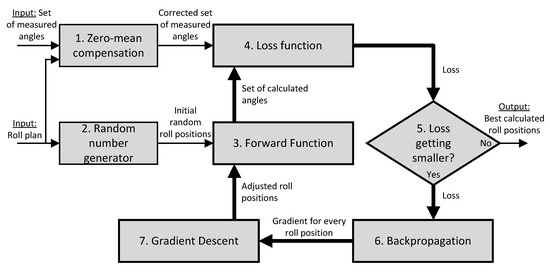
Figure 7.
Structure of the optimization-based algorithm.
- The zero-mean compensation is applied to the set of measured angles.
- A set of random roll positions is generated. Each roll receives a random position error with only a radial component.
- Forward Function: Using this set of roll positions and some trigonometry, the angles that an SCM would measure are calculated.
- Loss Function: The set of angles from the previous step are compared to the measured angles and the loss is calculated.
- If the loss has not stopped decreasing, continue the loop. Otherwise, end the loop and return the best set of roll positions.
- Backpropagation: Every mathematical operation that is applied to convert the roll positions into the loss is tracked and recorded. That allows to propagate the loss backwards through the computation graph, yielding gradients for each roll position with respect to the loss.
- Gradient Descent: Using the gradients from the previous step, each roll position is shifted by a small amount, reducing the loss and therefore bringing the calculated positions closer to the actual ones. With this new set of roll positions, repeat from Step 3.
The algorithm is programmed in Python, version 3.11.4. Using tools from the popular data science library PyTorch, version 2.6.0, the tracking of gradients, backpropagation and optimization steps are implemented. The underlined steps are explained in further detail in the following paragraphs.
3.3.1. Forward Function
In the context of the optimization-based algorithm, the conversion of n roll positions into tangential angles represents the forward function. Its equations are derived from the geometry in Figure 8. The figure shows two consecutive outer rolls with different radii at the coordinates and . To calculate the tangential angle , the distance
between the midpoints is calculated first using the Pythagorean theorem. The inverse tangent function is used to find
which represents the angle of the midpoint connection line. Note, that the numerator and denominator are chosen such that they yield positive results for this geometry. The equations still hold, however, when these differences are negative, for example, when . To consider the influence of the different radii, a residual angle
must be calculated. Finally, the tangential angle
can be determined. Evaluating these equations for every consecutive outer roll pair yields a set of tangential angles as the result of the forward function.
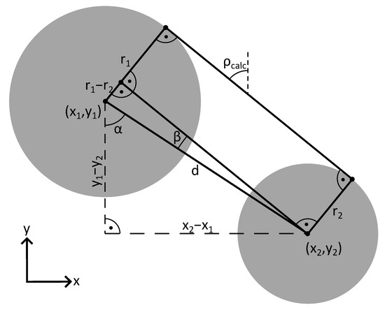
Figure 8.
Geometry of the forward function of the optimization-based algorithm. The conversion from roll positions to tangential angles is unambiguous and straightforward.
3.3.2. Loss Function
The next step in the loop is the calculation of the loss function. The loss function’s main task is to return a value that is representative of the difference between the measured angles and the result of the forward function. The sum of squared errors
fulfills this task. Here, and are the calculated and measured tangential angles between rolls k and .
Additionally, to ensure that the assumption of an ideally positioned footroll (roll 1) is met, the term
is included in the loss function. represents the radial component of the position error of roll k. Since the total value of the loss function gets minimized, will be close to zero after the optimization.
Lastly, a third term
is added to the loss function. Here, all positional roll errors are directly contributing to the loss function, which actually represents a conflict with the first term. However, this term is helpful because it prevents the algorithm from overfitting to the measured angles—which the geometric algorithms suffer from—and keeps the computed position errors within a reasonable range. This term must be carefully weighed using the factor such that the first and third term both contribute sensible amounts to the loss. By carefully choosing this factor, the optimization algorithm can be tuned to produce a good fit to the measured angles while simultaneously rejecting excessive measurement errors.
The complete loss function
is the sum of the three terms described above.
3.3.3. Backpropagation and Gradient Descent
PyTorch tracks the calculations applied in Steps 3 and 4, forming a computational graph from the roll positions to the loss. By calling the “backward”-function, PyTorch computes gradients for every node in the computational graph with respect to the loss, including the position errors.
Knowing the gradient of every roll position error with respect to the loss, gradient descent can be applied. With a learning rate of 0.6, each roll position error is slightly modified, consequently reducing the loss. The learning rate was determined iteratively, such that the algorithm always converges robustly and as fast as possible.
Since the loss function is constructed to minimize the difference between the calculated and measured tangential angles, the calculated roll positions are now closer to their real value and the loop is repeated with the modified set of roll positions.
To prevent infinite loops, the amount of loop repetitions is limited to a maximum of 20,000. In practice, the loss function usually stagnates after about 2000 iterations, leading to an early termination of the algorithm. To determine if the loss is stagnating, every 100 iterations, the trend (linear regression) of the loss in the last 20% of all iterations is considered. If the trend is not negative, the algorithm stops. Checking every 100 iterations is a compromise between the computational cost of calculating the trend and the desire to check often in order to stop as early as possible. Evaluating the trend over the last 20% of iterations turned out to be more robust and to lead to better early terminations than calculating it over a fixed number of last iterations. The final output of the algorithm is the set of roll positions that produced the lowest loss overall.
3.3.4. Error Weight Optimization
To finalize the development of the optimization-based algorithm, the optimal value for the error weight factor must be determined. This paragraph represents a slight anticipation of the following Section, since some results of the optimization-based algorithm must be analyzed in order to find the optimal error weight. To find the ideal value, the algorithm was tested under different combinations of amplitudes for constant and random angle measurement errors. The amplitudes of both error types range from 0° to 0.01° in four steps. For each of the resulting 16 cases, the error weight value was varied on a logarithmic scale from to 1. The error weight on the x-axis is plotted against the mean absolute calculation error of the roll positions. The result is shown in Figure 9.
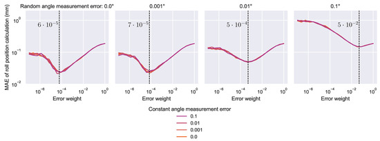
Figure 9.
Results of the error weight optimization for the optimization-based algorithm. It is effectively independent from the amplitude of the constant measurement error. The optimal error weight for each amplitude of random measurement error is marked.
The four different amplitudes of the random angle measurement errors are spread across the four diagrams while the different amplitudes of the constant angle measurement errors can be distinguished by color. The best value for the error weight for each of the 16 cases is found at the minimum of each graph.
The data suggest that the optimal error weight is effectively independent from the amplitude of the constant angle measurement error. This is due to the zero-mean compensation that is applied to the angle measurements, removing most of the constant error component. The amplitude of the random angle measurement error on the other hand strongly influences which value is ideal for the error weight. The best error weight values are marked in the diagram.
Experiments with SCM revealed that random angle measurement errors typically remain within 0.01° under real-world conditions. Therefore, the algorithm was optimized for this error range. When random measurement errors reach or exceed 0.1°, the calculation results become too inaccurate for practical application, making optimization for such cases unnecessary.
Based on this analysis, an error weight of was selected for use in subsequent experiments. The chosen weight also ensures acceptable performance even when random measurement errors are lower than 0.01° (see Figure 9).
4. Results and Discussion
In this Section, the three developed algorithms are tested and evaluated under different conditions regarding roll position and angle measurement errors. Additionally, the impact of the previously made assumptions is discussed. First, however, they are tested under ideal conditions to evaluate their baseline performance.
4.1. Baseline Performance
The ideal conditions for the baseline tests are:
- No constant angle measurement errors.
- No random angle measurement errors.
- No tangential roll position errors.
- No radial roll position errors.
The results are shown in Figure 10.
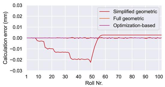
Figure 10.
Baseline performances of the algorithms. The y-axis represents the difference between the calculated and the actual radial component of the roll position error. Both the full geometric and optimization-based algorithm are effectively error-free. Even the simplified geometric algorithm only deviates about mm from the target values. Since it is based on the assumption that each roll has the same diameter, changes in roll diameter cause jumps in this diagram, for example, at rolls 14/15 and 33/34.
The simplified geometric algorithm yields calculation errors despite the ideal conditions. This is due to the simplifying assumptions that were made for this algorithm: neglecting the strand curvature and the varying roll diameters. The points at which the roll diameters change are visible as steps in the diagram. In the horizontal part of the machine (beginning at roll 57), both assumptions are valid, which is why this region shows no additional calculation errors. Despite these systematic calculation errors, the maximum calculation error of about mm is still small compared to the targeted accuracy, which proves the baseline functionality of the algorithm.
The full geometric algorithm shows no calculation error, as expected, since it does not make any simplifying assumptions about the machine and roll geometry.
Similar to the full geometric algorithm, the baseline performance of the optimization-based algorithm is nearly error free. However, due to the stochastic nature of this algorithm, some small deviations from the ideal solution are visible. In contrast to the deterministic geometric algorithms, which always yield the same solution under the same conditions, the optimization-based algorithm shows stochastic noise in its output.
4.2. Performance Under Error Influence
To evaluate the performance of the algorithms under non-ideal conditions, sets of roll positions with random position errors, including radial and tangential components, are generated. The radial components represent the target solution, which the algorithm will have to reproduce based on tangential angles. These are calculated from the roll positions using the same Equations (21)–(24) as in the forward function of the optimization-based algorithm. After that, artificial errors are applied to the angle values to simulate measurement errors. Two types of measurement errors can be applied: constant and random. Constant errors represent systematic measurement errors that can occur in the real world, for example, with a slightly tilted or miscalibrated angle sensor. They are applied by adding a constant value to every tangential angle. Random errors occur in the real world as measurement noise or mechanical vibrations. For these, a random distribution of errors is added to the angles.
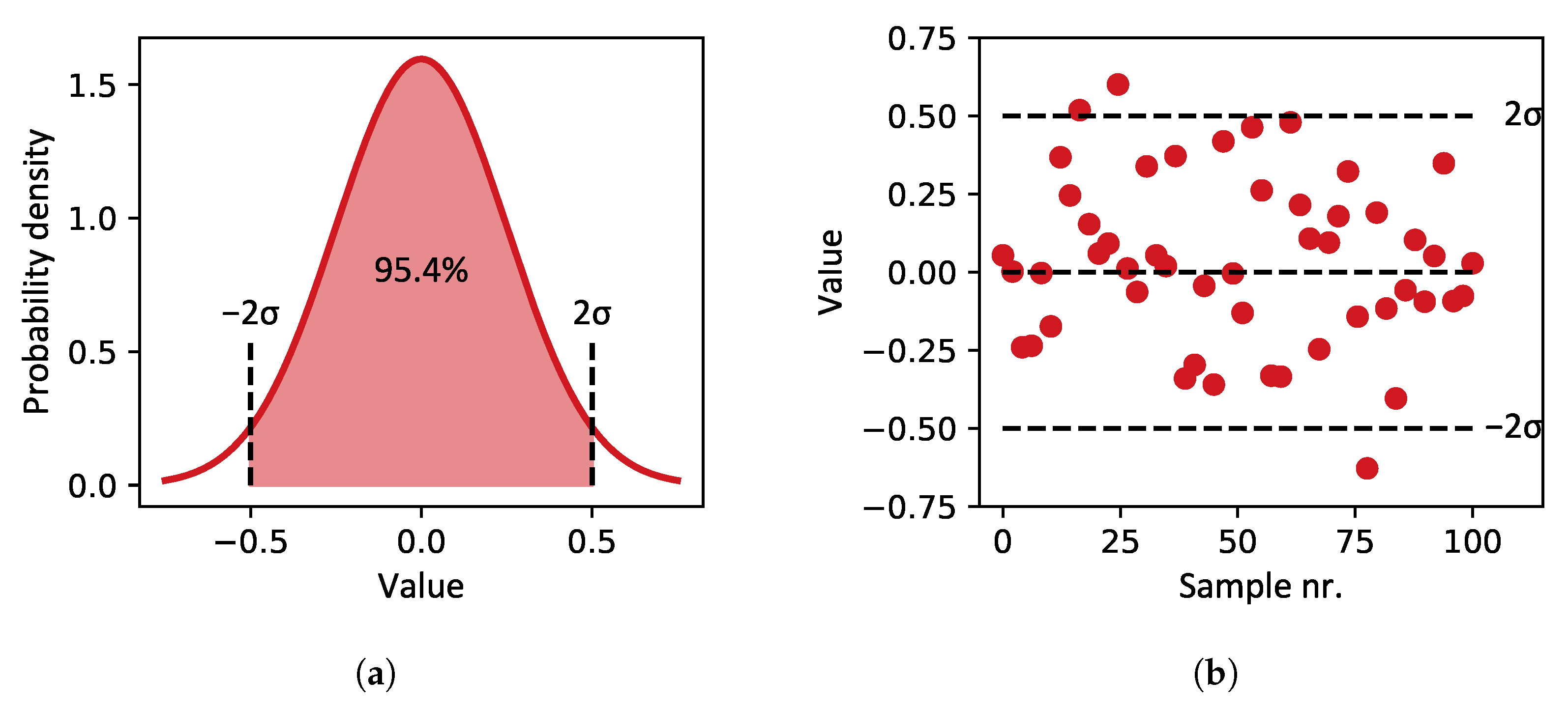
The underlying concept for random sets of values (position errors or measurement errors) is a normal distribution (see Figure 11). In this paper, the amplitude of a random distribution is defined as two times the standard deviation of that distribution, such that 95.4% of randomly sampled values lie within that amplitude.
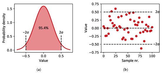
Figure 11.
(a) Normal distribution with an amplitude (two times standard deviation) of 0.5. A total of 95.4% of sampled values will fall within this amplitude. (b) Example of 100 values sampled from that distribution.
Each algorithm will be tested in five different experiments. Table 2 provides an overview of the experimental conditions.
Table 2.
Experimental conditions to test the algorithms.
The first four experiments reveal the susceptibility of the algorithms to each of the four types of errors. In the fifth experiment, the algorithms are tested under the influence of all error types at once, which is the most realistic case. The result of the fifth experiment will determine the best-performing algorithm. To keep the chapter to a reasonable size, only one error amplitude is tested in each experiment. The amplitudes represent plausible real-world values.
An amplitude of mm was chosen for the roll position errors according to the maximum tolerated errors by CCM operators. The amplitude of 0.01° was chosen for the angle measurement errors based on the targeted accuracy of SCM manufacturers and rough estimations of the measurement accuracy needed to achieve the desired position calculation accuracy. These error amplitudes are well suited to reveal the strengths and weaknesses of the algorithms, as will be demonstrated by the experimental results.
Every experiment is run 100 times for each algorithm in order to capture the behavior under different random error distributions. All 100 runs are shown in the same diagram to give an impression of the average, best and worst case performances.
In Experiment 1, the influence of a radial component in the roll position errors is investigated. It is expected that the results of this experiment are very similar to the baseline performance, since there are no measurement errors and the algorithms are designed to reproduce the radial components. However, as can be seen in Figure 12, the performance is much worse than the algorithm’s baselines.
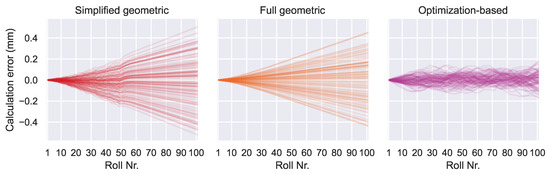
Figure 12.
Results of Experiment 1 with activated zero-mean compensation. The calculation errors are much worse compared to the baseline performance because the zero-mean compensation is detrimental in this scenario.
This result is due to the zero-mean compensation and an effect called “calculation error accumulation”. The roll position errors lead to differences between the measured tangential angles and the ideal tangential angles. The mean of this difference is not exactly equal to zero because only about 100 values were sampled from the random distribution and because the relationship between the roll positions and tangential angles is non-linear. The compensation method interprets this as a constant error component in the angle measurement and removes it. However, because there was no measurement error in the first place, this acts like an addition of a small constant error component to the angle measurements. Even though this added error is small, the performance deteriorates significantly due to calculation error accumulation.
Calculation error accumulation is indicated by a calculation error that rises nearly linearly over the length of the machine. The results from the geometric algorithms show this behavior in Figure 12. A constant measurement error in combination with the chain-like structure of the geometric algorithms are responsible here. At each step in the calculation chain, the constant component of the angle measurement error contributes to an error in the position calculation for the next roll. With each roll in the calculation chain, this error accumulates continuously, leading to the observed behavior. The optimization-based algorithm is much less affected because the third term in the loss function helps to keep the predicted positions errors small. This effect was also mentioned in [22,25].
To test the algorithms without the compensation, it is temporarily turned off and Experiment 1 is run again. The result is shown in Figure 13.
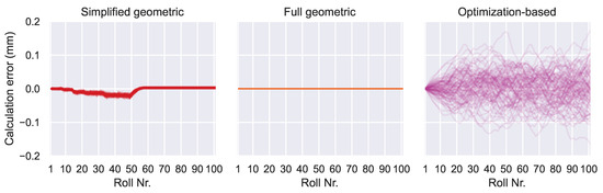
Figure 13.
Results of Experiment 1 without zero-mean compensation. As expected, the geometric algorithms performances are close or identical to their baseline performance. The optimization-based algorithm performs worse than its baseline because its error weight is tuned to non-zero random angle measurement errors and tends to underestimate the roll position errors in this scenario.
The simplified geometric algorithm now performs near its baseline again, with some additional noise from the random roll position errors. As expected, the full geometric algorithm returns to its error-free baseline performance. The optimization-based algorithm performs worse in this scenario, due to the third term in its loss function. The error weight was tuned to a random component in the angle measurement errors of 0.01°, which leads to a worse, but still acceptable performance.
This experiment proves the general functionality of each algorithm. Especially, the geometric algorithms perform excellently under these ideal measurement conditions.
In Experiment 2, the influence of tangential components with an amplitude of mm in the roll position errors is investigated. In practice, the tangential components are expected to have a similar distribution and amplitude as the radial components. However, only the radial components are considered by the algorithms, leading to an unavoidable calculation error. Therefore, the computational errors that result from this experiment limit the overall achievable accuracy of each algorithm and represent an important quality measure. Nevertheless, the tangential components have a lower influence on the measured angles than the radial components and thus the effect is expected to be comparatively low. Figure 14 shows the result of the experiment. It is apparent that the random tangential components have a noticeable influence on the calculation accuracy. The calculation error of the geometric algorithms stays below mm in every case and 90% of calculation errors lie below mm. For the desired accuracy of mm, this result leaves little room for the influence of other factors. The optimization-based algorithm seems to be robust against tangential errors, with a maximum calculation error of mm and 90% of calculation errors below mm, leaving room for other influences.
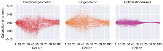
Figure 14.
Results of Experiment 2 with zero-mean compensation.
Starting at roll 57, the horizontal section of the plant is recognizable in all diagrams. That is expected, since the tangential error components have no influence on the tangential angles in the horizontal section of the plant when the radial components are zero. Still, some calculation error accumulation is visible for the geometric algorithms. It is not affected by error accumulation and is able to minimize the computation error in the horizontal section. Since the radial components of the roll errors are actually zero in this experiment, the third term of the loss function has a positive impact.
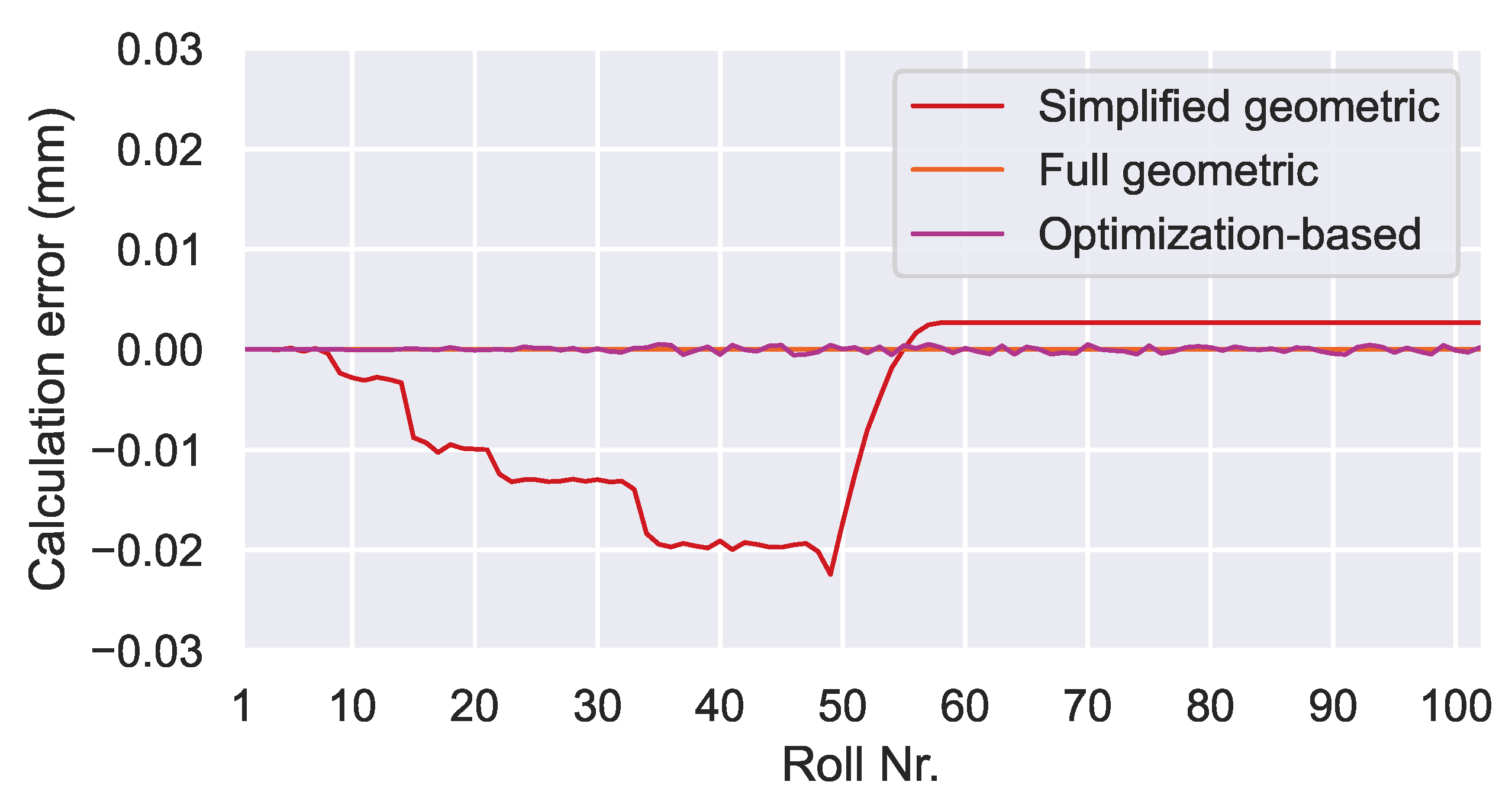
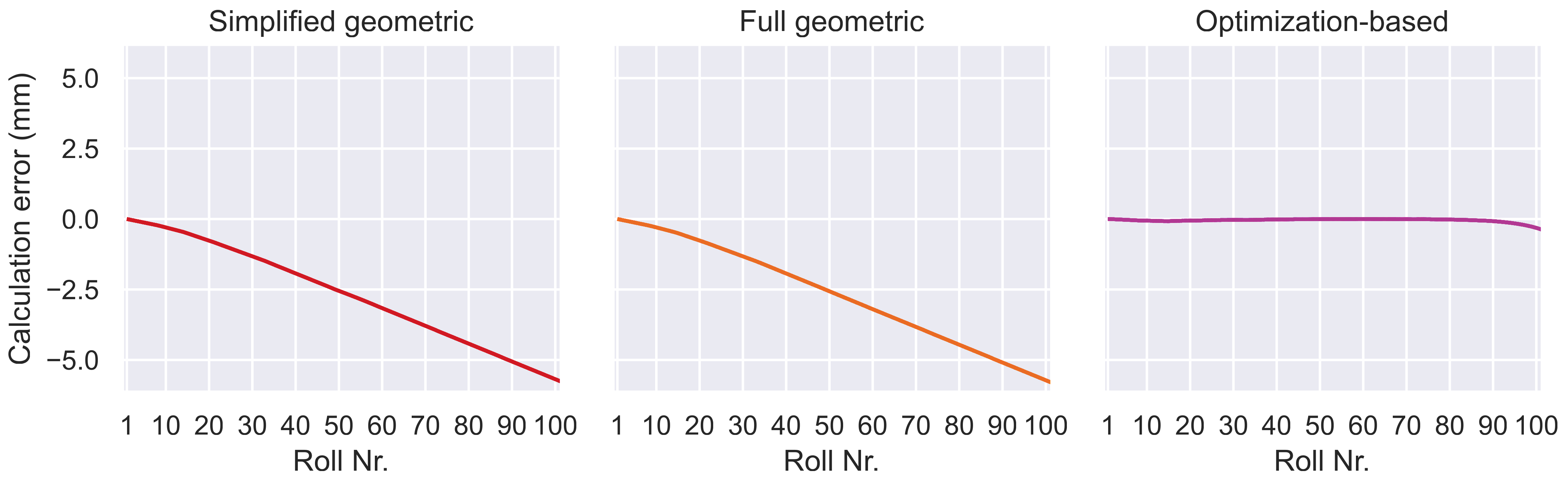
In Experiment 3, the influence of a constant angle measurement error of 0.01° is shown. Since the angle measurement error is purely constant in this experiment, the zero-mean compensation corrects it entirely. This leads to the algorithms performing at their baseline performance which is not shown again. Rather, to demonstrate its effect, the compensation was temporarily deactivated for this experiment. The results are shown in Figure 15 and demonstrate the detrimental effect of error accumulation and the necessity of the compensation. Both geometric algorithms show effectively the same result, which is an almost linearly rising calculation error. Towards the end of the machine, this error accumulates to a value close to mm, which is unacceptable. This gave impetus to the development of the optimization-based algorithm in the first place.
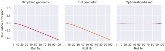
Figure 15.
Result of Experiment 3 without zero-mean compensation. Without the compensation, the geometric algorithms suffer heavily from the influence of a constant error in the angle measurements.
The optimization-based algorithm shows a much better performance, even without the zero-mean compensation. This is due to the third term in the loss function that tries to minimize the roll position. If would be set to zero, the result of the optimization-based algorithm would look like the result of the geometric algorithms. It is worth noting that between rolls 90 and 102, a small amount of the effect also affects the optimization-based algorithm.
This experiment demonstrates the importance of the zero-mean compensation. It shows how susceptible the geometric algorithms are to constant components in the angle measurement errors. It also becomes clear that the additional term in the loss function of the optimization-based algorithm improves the robustness against this type of error significantly. This is important because in the presence of a random distribution of errors, the compensation method is not able to completely remove the constant component of angle measurement errors. The geometric algorithms will accumulate the residual error while the third term of the optimization-based algorithm will suppress most of it. This effect seems to be the main reason for the superior results of the optimization-based algorithm.
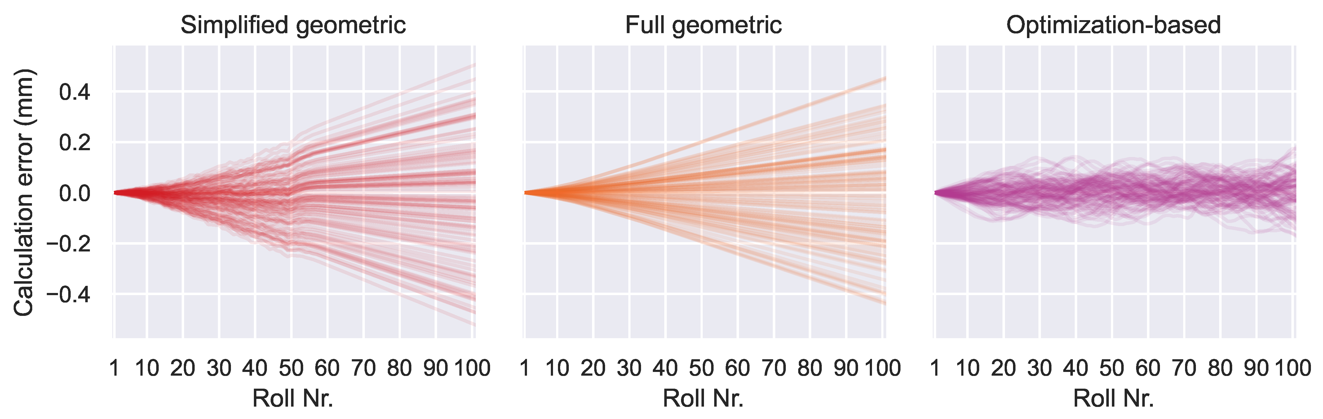
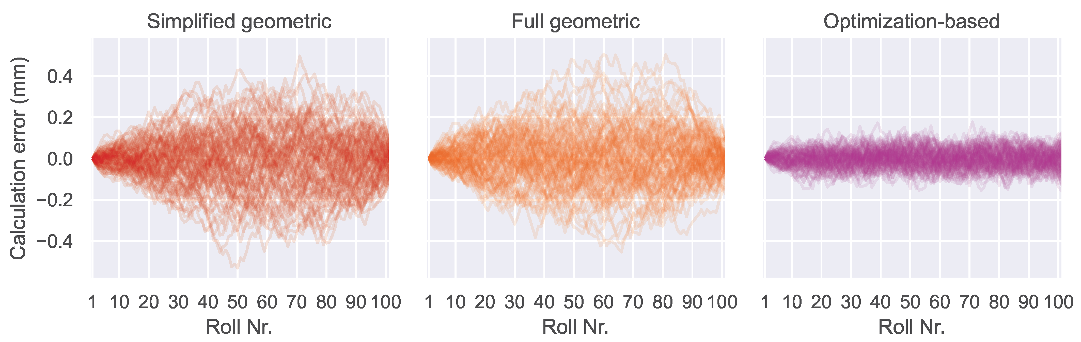
In Experiment 4, all error types except random angle measurement errors are set to zero. The zero-mean compensation is activated, even though it would not show a strong effect in this experiment, since the mean of the randomly sampled angle measurement errors is near zero by definition of the normal distribution. The result is shown in Figure 16.
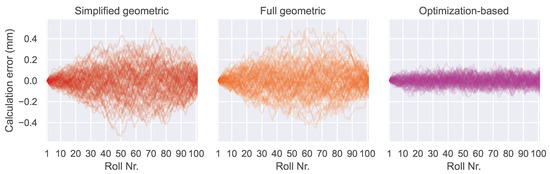
Figure 16.
Result of Experiment 4 with zero-mean compensation. The differences between the geometric algorithms differences are insignificant compared to the influence of the random angle measurement errors. In this experiment, the strengths of the optimization-based algorithm show clearly.
Both geometric algorithms show similar performance because the overall calculation error is much bigger than the systematic errors of the simplified algorithm. Their calculation errors mostly stay below mm. The performance of the optimization-based algorithm is significantly better, with calculation errors mostly staying below mm. No error accumulation is visible, since the error type is purely random.
None of the algorithms can keep all calculation errors below the targeted mm. This is the worst result of the four experiments (with activated zero-mean compensation), indicating that this error type is the primary cause of calculation errors.
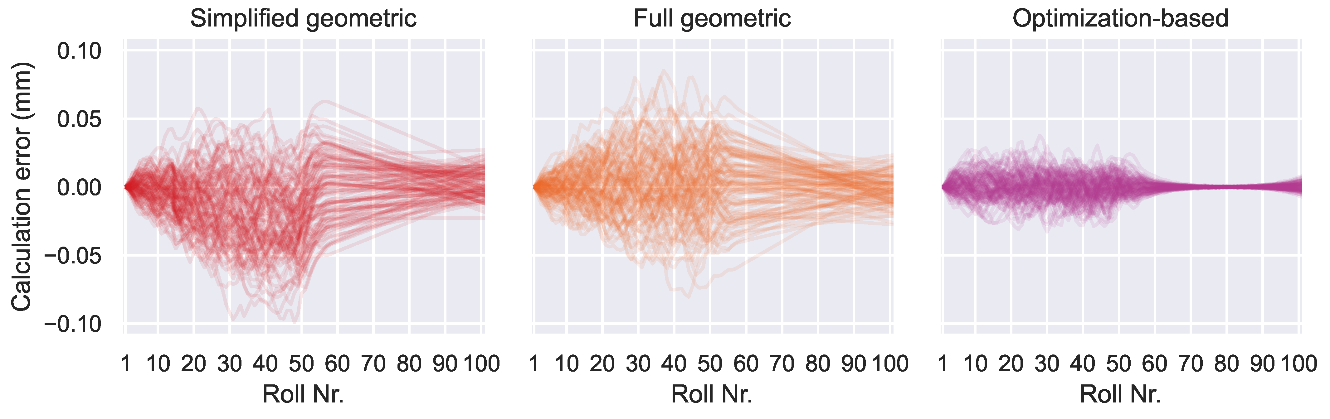
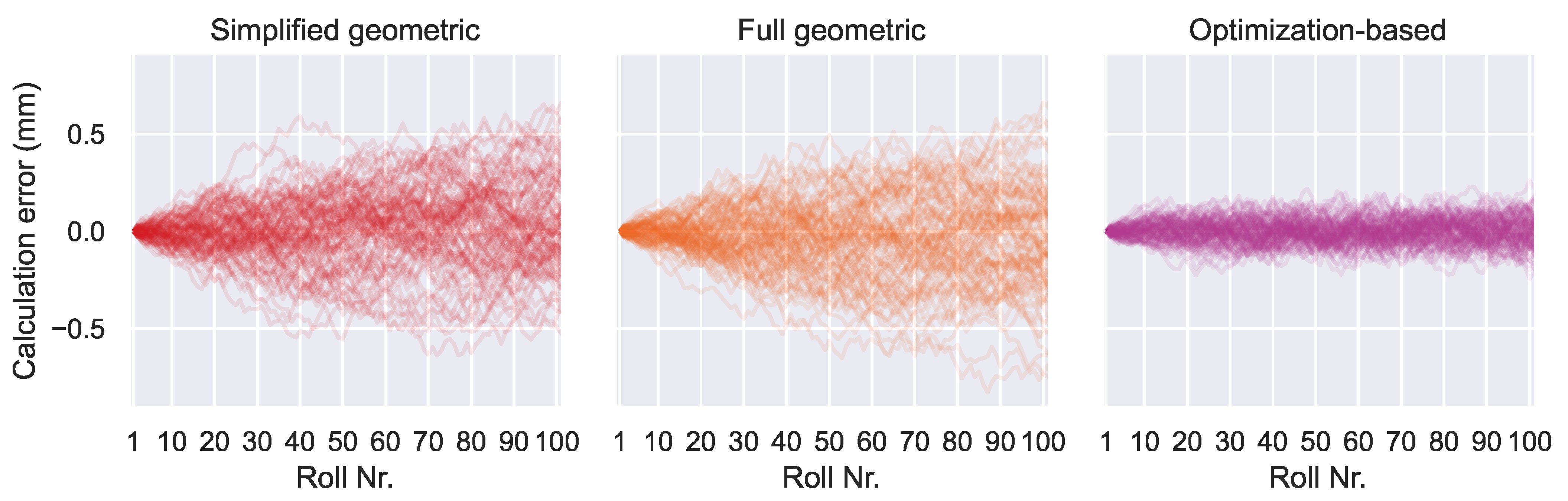
Experiment 5 combines all errors from the previous four experiments. This represents the most realistic case, since the error types never occur isolated in the real world. The first four experiments were useful to explore and understand the algorithm’s behavior under different conditions. Experiment 5 will show which algorithm works best in a real world scenario. Figure 17 shows the result.

Figure 17.
Results of Experiment 5 with zero-mean compensation. The result is similar to Experiment 4, suggesting that random angle measurement errors are the dominant cause of computational errors.
The results of Experiment 5 are similar, but slightly worse than Experiment 4, indicating again that the influence of random angle measurement errors is dominant. Looking at the previous experiments, the reason why the other error types have minor influence becomes apparent: The radial components of the roll position errors do not have a strong influence because the algorithms are designed to calculate those. The tangential components of the roll position errors only have a small influence on the measured angles and thus on the algorithms. Lastly, the constant angle measurement errors are effectively removed by the zero-mean compensation. This leaves only the random angle measurement errors to have a strong impact on the performance of the algorithms.
The results of all five experiments are summarized in Figure 18.
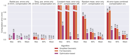
Figure 18.
Results comparison for all experiments. Three metrics were extracted: the biggest computation error that occured in 100 runs, the threshold under which 90% of the computation errors occured and the mean computation error. The first four diagrams illustrate the sensitivity of each algorithm regarding the four error types. In the first and third experiment, the zero-mean compensation was turned off to better illustrate the algorithms properties. The rightmost diagram contains the result of Experiment 5, where all error types were combined to simulate a realistic scenario.
4.3. Failure Modes
As shown in the previous experiments, the random angle measurement errors are the main cause of computational errors. However, the experiments do not show at which error amplitude the algorithms fail. To answer this question, each algorithm was tested with an increasing random angle measurement error until the mean and the 90 percentile of the computational error exceeds the target of mm, respectively. The amplitudes of both components of the random roll position errors are kept constant at mm. The constant angle measurement error is also kept constant at a value of 0.01°. Due to the zero-mean compensation, the amplitude of the constant angle measurement error has no effect in this case and could be set to an arbritrary value without altering the result. These error amplitudes are identical with Experiment 5 to keep the results, which are shown in Table 3, comparable.
Table 3.
Failure modes for each algorithm. Each value represents the maximum amplitude of random angle measurement error in order to keep the error metric below mm. A dash indicates that no error amplitude results in the metric below mm.
The results show clearly that only the optimization-based algorithm reaches the desired computational accuracy given the current measurement abilities of SCM. None of the geometric algorithms is able to reach the desired accuracy in the 90 percentile metric at all, which is due to the negative influences of the roll position errors (see Experiments 1 and 2). Even in the case of perfect angle measurements, their 90 percentile computation error stays above mm. This influence is also the reason why none of the algorithms is able to keep the maximum computational error under the targeted mm. However, this metric is prone to random outliers and the 90 percentile metric is the most significant for the practical application.
4.4. Influence of the Footroll
To provide an anchor point to the global coordinate system for the algorithms, the position of the footroll is assumed to be known and error free. In practice though, even the closely monitored footroll is never perfectly aligned. Any error in the footrolls position causes a shift in this anchor point and thus a calculation error for every roll that is equal to the position error of the footroll. This can be imagined as a virtual shift of the entire machine. However, this does not pose a problem. Shifting the entire machine does not affect how the rolls act on the strand. The positions of the rolls relative to the footroll, the strand and each other—which is the relevant part regarding the quality—are captured by the algorithms nonetheless.
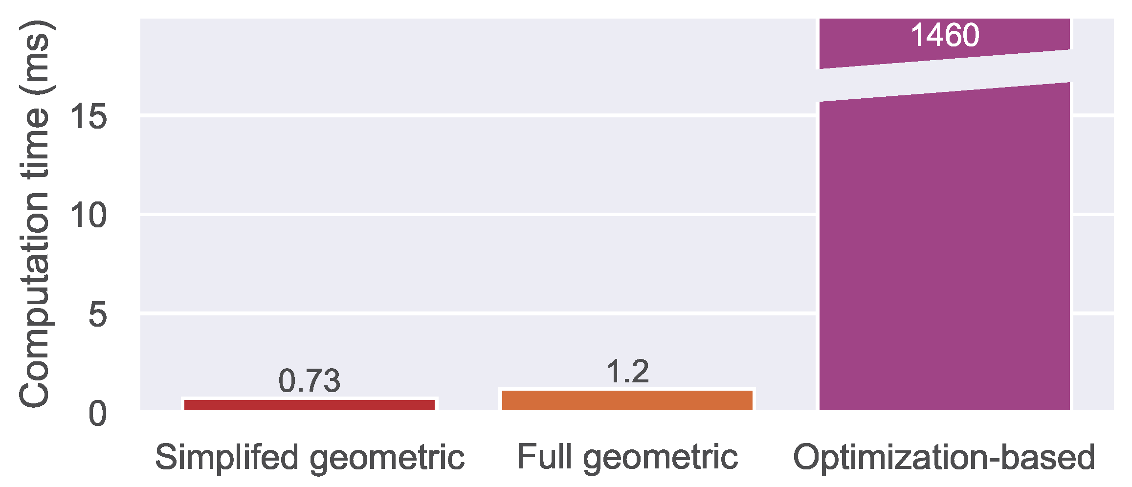
4.5. Computational Cost
Before the best algorithm can be determined, the computational cost must be evaluated. The average runtimes of each algorithm were measured and are shown in Figure 19. Since both geometric approaches share the same general approach, they result in a similar runtime. While the simplified approach needs a bit less than a millisecond, the full geometric algorithm takes a bit longer than a millisecond. Due to the iterative nature of the optimization-based algorithm, where all calculations are performed about 2000 times, the runtime is about 1000 times longer ( s). In the context of the application, this computation time is perfectly acceptable and it is vastly outweighed by the algorithm’s performance.
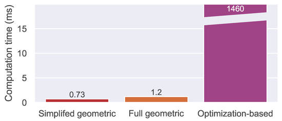
Figure 19.
Comparison of computation times for of each algorithm.
5. Conclusions
Continuously monitoring and improving the alignment condition of a CCM is a critical task to ensure a consistent and high-quality production of steel. Measuring the alignment is still a challenge today and the angle measurement data from SCMs often contain systematic and stochastic errors. The contribution of this paper is the development of an algorithm that robustly and accurately converts the angle measurements into the Cartesian coordinates of the rolls with the desired accuracy of mm. Three different approaches were developed, tested and compared. The first two approaches are purely geometric and rely on trigonometry, while the third approach is based on the gradient descent optimization algorithm.
Under ideal conditions, all algorithms show very good performance. The simplifed geometric algorithm yields a computational error of around mm, while the full geometric and the optimization-based algorithm produce effectively no computational error.
Five different experiments were conducted to investigate the susceptibility of the algorithms to the four error types that may occur in the real world: radial and tangential components in roll position errors as well as constant and random components in angle measurement errors. The experiments showed that the influence of roll position errors (radial and tangential) on the accuracy of the algorithms is small and remains in an acceptable range. Constant angle measurement errors on the other hand lead to large error accumulation within the geometric approaches. A constant angle measurement error as small as 0.01° leads to computation errors of almost 6 mm. However, utilizing a zero-mean compensation method effectively mitigates this effect.
Therefore, random angle measurement errors remain as the dominant challenge for the algorithms, since these cannot be compensated or neglected. Under the influence of random angle measurements with an amplitude of 0.01°, the algorithms yield 90 percentile computational errors of mm, mm and mm, respectively.
The fifth experiment, which applies all four types of errors simultaneously, represents the most realistic and representative case. The results showed that the optimization-based algorithm performs, on average, about three times better than the geometric algorithms: mm, mm and mm 90 percentile computational error, respectively. It is the only algorithm that reaches the desired accuracy. However, it has to be noted that the performance of the optimization-based algorithm relies on the weight factor , which depends on the amplitude of random measurement errors. This amplitude must be determined experimentally and the weight factor must be tuned for any given SCM and CCM in order to yield the shown results. Nevertheless, the gains in calculation accuracy over the geometric algorithms justify the effort.
The next step in the continuation of this research is a test of the algorithms on an actual CCM. To evaluate the results of the algorithms, the actual alignment of the plant would need to be determined using a laser scanner or total station prior to the measurement with the SCM. Additionally, further improving the angle measurement accuracy of SCM would be beneficial because the experiments showed that an accuracy of 0.01° is just about enough to reach the targeted position calculation accuracy with the optimization-based algorithm.
Author Contributions
Conceptualization, R.R. and M.J.; methodology, R.R.; software, R.R.; writing—original draft preparation, R.R.; writing—review and editing, N.A. and M.J.; visualization, R.R.; supervision, M.J.; project administration, N.A. and M.J.; funding acquisition, N.A. and M.J.; All authors have read and agreed to the published version of the manuscript.
Funding
This research was funded by the Central Innovation Programme for small and medium-sized enterprises (SMEs) of the German Federal Ministry for Economic Affairs and Climate Action. Grant number KK5149906DF2.
Data Availability Statement
Due to the confidentiality agreed upon in the cooperation agreement of the research project, the data used and the source code of the algorithms presented in this article are not readily available. Requests to access the data and source code should be directed to Mohieddine Jelali.
Acknowledgments
The authors thank Loui Al-Shrouf for his kind support.
Conflicts of Interest
Author Nils Albersmann was employed by the company Gassen Instruments GmbH. The remaining authors declare that the research was conducted in the absence of any commercial or financial relationships that could be construed as a potential conflict of interest. The authors declare that this study received funding from the German Federal Ministry for Economic Affairs and Climate Action. The funder was not involved in the study design, collection, analysis, interpretation of data, the writing of this article or the decision to submit it for publication.
Abbreviations
The following abbreviations are used in this manuscript:
| CCM | continuous casting machine |
| SCM | strand condition monitoring system |
References
- Cemernek, D.; Cemernek, S.; Gursch, H.; Pandeshwar, A.; Leitner, T.; Berger, M.; Klösch, G.; Kern, R. Machine learning in continuous casting of steel: A state-of-the-art survey. J. Intell. Manuf. 2022, 33, 1561–1579. [Google Scholar] [CrossRef]
- Thomas, B.G. Review on Modeling and Simulation of Continuous Casting. Steel Res. Int. 2018, 89, 1700312. [Google Scholar] [CrossRef]
- Norrena, J.; Louhenkilpi, S.; Visuri, V.V.; Alatarvas, T.; Bogdanoff, A.; Fabritius, T. Assessing the Effects of Steel Composition on Surface Cracks in Continuous Casting with Solidification Simulations and Phenomenological Quality Criteria for Quality Prediction Applications. Steel Res. Int. 2023, 94, 2200746. [Google Scholar] [CrossRef]
- Kong, Y.; Chen, D.; Liu, Q.; Long, M. A Prediction Model for Internal Cracks during Slab Continuous Casting. Metals 2019, 9, 587. [Google Scholar] [CrossRef]
- Zou, L.; Zhang, J.; Han, Y.; Zeng, F.; Li, Q.; Liu, Q. Internal Crack Prediction of Continuous Casting Billet Based on Principal Component Analysis and Deep Neural Network. Metals 2021, 11, 1976. [Google Scholar] [CrossRef]
- Amratav, N.; Kumar, K.; Pillai, M. Computer Simulation of Continuous Casting Processes: A Review. Adv. Mater. 2021, 10, 31–41. [Google Scholar] [CrossRef]
- Popa, E.M.; Kiss, I. Assessment of Surface Defects in the Continuously Cast Steel. In Acta Technica Corviniensis; European Virtual Institute for Speciation Analysis (EVISA): Pau, France, 2011; pp. 109–115. [Google Scholar]
- Adamenko, O.; Martynov, O. Checking the Stands of the Continuous Casting Machine with a Total Station. In Proceedings of the 23rd SGEM International Multidisciplinary Scientific GeoConference, Albena, Bulgaria, 3–9 July 2023. [Google Scholar] [CrossRef]
- Sotnikov, A.L.; Sholomitskii, A.A.; Strichenko, S.M. Study of the Principles for Ensuring the Accuracy of CCM Design Parameters. IOP Conf. Ser. Mater. Sci. Eng. 2020, 969, 012061. [Google Scholar] [CrossRef]
- Spinelli, D. Laser Alignment for the Caster Machine Repair Aisle. In AISE Steel Technology; Association of Iron and Steel Engineers: Hamilton, ON, Canada, 2002; pp. 46–47. [Google Scholar]
- Miłkowska-Piszczek, K.; Falkus, J. Control and Design of the Steel Continuous Casting Process Based on Advanced Numerical Models. Metals 2018, 8, 591. [Google Scholar] [CrossRef]
- Tokuda, M. Development of Diagnosis System for Roll Alignment and Roll Rotation in Continuous Casting Process. Tetsu-to-Hagané 2001, 87, 593–599. [Google Scholar] [CrossRef]
- Lee, S.J.; Cho, K.H.; Kang, S.E. Development of strand condition diagnostic system of continuous slab caster by using wireless telemetry. In Proceedings of the ISSPA ’99 Fifth International Symposium on Signal Processing and Its Applications, Brisbane, Australia, 22–25 August 1999; pp. 579–582. [Google Scholar] [CrossRef]
- Ozgu, M.R. Continuous caster instrumentation: State-of-the-art review. Can. Metall. Q. 1996, 35, 199–223. [Google Scholar] [CrossRef]
- Pritchard, W.D.N.; Hyde, G. The Monitoring of the Alignment of Continuous Casting Machines. In COMADEM 89 International: Proceedings of the First International Congress on Condition Monitoring and Diagnostic Engineering Management; Rao, R.B.K.N., Hope, A.D., Eds.; Springer: Boston, MA, USA, 1989; pp. 187–193. [Google Scholar] [CrossRef]
- Pattery, P.A. Slab Caster Roller and the Significance of Its Design in the Production of Slabs; University Duisburg Essen: Duisburg, Germany, 2005. [Google Scholar]
- Liu, W.; Xie, Z.; Chen, H. Modeling and simulation of quality analysis of internal cracks based on FTA in continuos casting billet. In Proceedings of the IEEE 2nd International Conference on Computing, Control and Industrial Engineering, Wuhan, China, 20–21 August 2011; IEEE: Piscataway, NJ, USA, 2011; pp. 359–362. [Google Scholar] [CrossRef]
- Gerz, F.; Rosenthal, R.; Albersmann, N.; Jelali, M. Research Project HeRoS—Measurement and Evaluation System for the Alignment of Outer Rolls of Continuous Casting Machines: Final Report; TH Köln—Cologne University of Applied Sciences: Cologne, Germany, 2025. [Google Scholar]
- Gorainov, S.; Plociennik, C.; Krasilnikov, A. Technologischer Assistent für Die Automatisierte Diagnostik des Zustandes Einer Stranggießanlage. Available online: https://www.researchgate.net/publication/318589970 (accessed on 30 April 2025).
- Lang, O.; Mittermair, A.; Winkler, K. Smart Production with New Measure Device for Continuous Casting. Available online: https://www.researchgate.net/publication/355913872 (accessed on 30 April 2025).
- Han, Z.; Shi, H.; Liu, Y.; Ba, L.; Yuan, Q.; Yang, M.; Gao, X. Framework for remaining useful life prediction of casting roller in continuous casting machine based on digital twin. In Proceedings of the 2021 IEEE International Conference on Software Engineering and Artificial Intelligence (SEAI), Xiamen, China, 11–13 June 2021; pp. 17–22. [Google Scholar] [CrossRef]
- Sholomitskii, A.; Sotnikov, A. Position Control and Alignment of the CCM Equipment. Mater. Sci. Forum 2019, 946, 644–649. [Google Scholar] [CrossRef]
- Sigma3D. Digitalisierung Einer Stranggießanlage. Available online: https://www.sigma3d.de/referenzen/digitalisierung-einer-stranggiessanlage-1/ (accessed on 29 April 2025).
- von Wyl, H. Project CHECKER: Work Report, Duisburg, Germany. Unpublished work. 2021.
- POWER MnC Co., Ltd. Caster Strand Monitoring System: Roll Checker. Available online: www.powermnc.com (accessed on 30 April 2025).


Disclaimer/Publisher’s Note: The statements, opinions and data contained in all publications are solely those of the individual author(s) and contributor(s) and not of MDPI and/or the editor(s). MDPI and/or the editor(s) disclaim responsibility for any injury to people or property resulting from any ideas, methods, instructions or products referred to in the content. |
© 2025 by the authors. Licensee MDPI, Basel, Switzerland. This article is an open access article distributed under the terms and conditions of the Creative Commons Attribution (CC BY) license (https://creativecommons.org/licenses/by/4.0/).