Learning Individualized Hyperparameter Settings

Abstract

The performance of optimization algorithms, and consequently of AI/machine learning solutions, is strongly influenced by the setting of their hyperparameters. Over the last decades, a rich literature has developed proposing methods to automatically determine the parameter setting for a problem of interest, aiming at either robust or instance-specific settings. Robust setting optimization is already a mature area of research, while instance-level setting is still in its infancy, with contributions mainly dealing with algorithm selection. The work reported in this paper belongs to the latter category, exploiting the learning and generalization capabilities of artificial neural networks to adapt a general setting generated by state-of-the-art automatic configurators. Our approach differs significantly from analogous ones in the literature, both because we rely on neural systems to suggest the settings, and because we propose a novel learning scheme in which different outputs are proposed for each input, in order to support generalization from examples. The approach was validated on two different algorithms that optimized instances of two different problems. We used an algorithm that is very sensitive to parameter settings, applied to generalized assignment problem instances, and a robust tabu search that is purportedly little sensitive to its settings, applied to quadratic assignment problem instances. The computational results in both cases attest to the effectiveness of the approach, especially when applied to instances that are structurally very different from those previously encountered.

1. Introduction

Most optimization algorithms, and consequently most AI/machine learning (ML) solutions, have an effectiveness that depends heavily on the values imposed on high-level guiding parameters, usually called hyperparameters. Choosing a bad setting can result in anything from needing more time to reach the solution to being denied any success in the search. Therefore, the identification of an effective hyperparameter setting is configured as a higher-level optimization task, instrumental in obtaining a successful application of the search algorithm of interest.

Over the last few decades, a rich literature has developed proposing methods for automatically estimating parameter settings, using approaches ranging from purely statistical to tailored heuristics. Two main lines of research have emerged, one aiming at identifying a robust setting that makes an algorithm of interest effective on all (most) instances of the problem to be optimized, and one tailoring the setting to each specific instance. In fact, it is a common practical awareness that different instances of the same problem can require very different computational efforts to solve, even if their dimensions are the same. The computational complexity theory justifies such diversity among problems, but it cannot be declined at the instance level, while the “no free lunch” theorem is valid even among instances [1]. More efficient solution processes could therefore benefit from different settings tailored at the individual instance level, but the marginal benefits must be weighed against the costs of achieving them.

This work considers both objectives, building upon automatic configurators but taking into account the large diversity among instances of the same problem. The approach we follow differs from that usually proposed in the literature of individual settings in that we adapt prelearned settings to each specific instance, relying on neural networks, specifically multilayer perceptrons (MLPs), to obtain the adapted settings in real time. Specifically, the methodology we present makes use of state-of-the-art automatic algorithm configurators to generate datasets of instance/setting pairs to be processed by the neural module. The generalization and abstraction capabilities of the neural component are used to obtain instance-specific hyperparameter settings for out-of-sample instances.

We assume that the different computational requests coming from different instances are due to different structures in the data distribution at the instance level and use this assumption to derive a pipeline that allows us to tailor the parameter setting of a given search algorithm to single, previously unforeseen instances.

It is clearly ineffective to propose raw instances as learning bases, so we rely on sets of descriptive statistics computed on both in-sample and out-of-sample (i.e., train and test) instances and pass them as input to the neural module. The pipeline starts by computing a set of descriptive statistics on the available instances, possibly filtering them, and applying a state-of-the-art configurator to different subsets of structurally similar instances. This produces a dataset of instance/setting pairs that can be used to instantiate learning. The learning module consists of a multilayer perceptron, whose abstraction and generalization capabilities are well known, and which is used in this case to abstract the mapping between instance statistics and setting, so that when a new instance is proposed, its statistics are computed and fed as input to the MLP, which in turn outputs the individualized setting.

We applied this pipeline to two different well-known combinatorial optimization heuristic algorithms whose code was made available by the authors and used it to solve two different problems. First, we considered a Lagrangian matheuristic [2,3], an algorithm that is very sensitive to its settings, and applied it to generalized assignment problem (GAP) instances. Second, we tested a robust tabu search [4], an algorithm that is considered robust precisely because of its relative insensitivity to hyperparameter settings, and applied it to quadratic assignment problem (QAP) instances.

The paper is structured as follows. Section 2 provides an overview of the state of the art in robust and instance-level parameter setting optimization. Section 3 details the problems we considered in this study and the algorithms we used to solve them and introduces the parameters of these algorithms that need to be set. Section 4 describes the pipeline we propose, including the stages of feature selection, possibly data augmentation, MLP learning, and parameter setting generation. Finally, Section 5 contains the computational results obtained in our study, and Section 6 draws some conclusions from the results obtained.

2. Related Literature

State-of-the-art optimization algorithms typically have a large number of parameters that need to be modified to ensure their performance. Traditionally, the identification of an effective setting has been achieved through a manual, experimental approach, mostly guided by the experience of the algorithm designers. However, manual exploration of the combinatorial space of parameter settings is tedious and tends to produce unsatisfactory results. Expectedly, the manual search can be less efficient than automatic procedures, so automatic configurators have been proposed for use when very high performance is required. Automatic or at least computer-assisted configuration has evolved along a line that tries to identify robust settings to be used on all problem instances, and along a second line that tries to propose individualized settings. There are several surveys that cover these topics [3,5,6,7].

Configurators of the first type [8,9,10,11,12] typically assume that an instance set of diverse representative instances is available, and specific methods are applied to the set to derive a robust setting that is effective on all of them, and thus hopefully on other instances of the same problem. Widely used systems in this group include ParamILS and irace, besides generic nonlinear optimization algorithms such as the Nelder–Mead simplex, swarm optimization [13], Bayesian optimization [14], or a random search [15] applied to this specific task.

ParamILS [11] is an iterated local search (ILS) algorithm that works in the search space of the parameters. It works on categorical parameters; therefore, real and integer parameters must first be converted to discrete values. After a possibly random initialization, a local search is started. The local search in ParamILS is a first-improvement local search, based on a one-exchange neighborhood, which can only change one parameter at a time. Each time a move finds a new improvement, it takes it and continues the search until all neighborhoods are examined or the budget is exhausted. At that point, the better of the current or previous local minima is kept, and the last solution is perturbed to reinitialize the search. ParamILS can be used for run-time configurations because it implements a procedure called adaptive capping, which prunes the search early to evaluate potentially poor-performing configurations, greatly reducing computation time.

The irace package [12] implements the so-called iterated race method, which is a generalization of the iterated F-race method for the automatic configuration of optimization algorithms [16]. irace is based on three successive phases. In the first phase, it generates candidate configurations using an appropriate statistical model. In the second phase, it selects the best candidate configurations using a race method based on either F-race or a paired Student’s t-test. Third, it updates the system’s probability model to give the most promising configurations a higher probability of being used. The general process starts by generating configurations within the user-specified value intervals for each parameter and subjecting them all to a race. In the race, configurations are evaluated on a first instance of the provided instance set, then on the second, and so on. As soon as a configuration is judged to be bad, it is eliminated, and the search continues until a small subset, by default four, of configurations survive, which are proposed in the output.

These algorithms represent the state of the art for robust setting optimization. The literature on individualized configuration uses them as a module of a more complex process, as our approach suggests as well.

Individualized tuning itself has different goals and follows different approaches. One approach is adaptive configuration, where parameter values are adjusted during the optimization process based on the performance of the algorithm [5]. This was pioneered by evolution strategies [17,18] and has received considerable attention since then but falls outside the scope of our research.

Even if we narrow the focus to static settings that do not change values during the search, there is a second subdivision to be made, namely between configurators that select the most promising solution algorithm, or part thereof, from a portfolio of candidate algorithms [19], and those that work on a single algorithm and optimize its parameters.

Individualized algorithm selection has been more extensively studied and has proven to be able to significantly improve the state of the art in some notable combinatorial problems, including propositional satisfiability [20] and the traveling salesman problem [21]. Prominent systems in this area are hydra [22] or llama [23], which are primarily algorithm portfolio selection systems, where the included automatic parameter configurator passes the task to optimizers such as ParamILS. Another interesting effort in the area of algorithm selection is the instance space analysis for algorithm testing [24], a proposal to structure the analysis of instance complexity and the degree of coverage of the universe of instances of a given problem guaranteed by the available test sets.

Research on optimizing parameters of a single algorithms, which has been named per-instance algorithm configuration (PIAC) [6], has seen less contributions. It typically involves two phases: an offline phase, during which the configurator is trained, and an online phase, in which the configurator is run on given problem instances. The result of the second phase is a parameter configuration determined on the features of the specific instance to be solved. We remark the difference from a standard algorithm configuration, which typically produces a single configuration that is then used on all presented instances.

The state of the art in PIAC is currently represented by ISAC (instance-specific algorithm configuration) [25]. Its general approach is the same as that described above or in instance space analysis, and as the one we adopted in our proposal as well. First, the available benchmark instances are clustered into distinct sets based on the similarity of their feature vectors as computed by a geometric norm. Then, assuming that instances with similar features behave similarly under the same algorithm, some kind of search is used to find good parameters for each cluster of instances. Finally, new instances are presented, and the optimized settings are used to determine the one to use for that instance. The way this is done may vary across systems. ISAC uses a g-means algorithm to cluster the training instances, and when a new instance is shown, it checks if there is a cluster whose center is close enough to the feature vector of the input. If so, the parameters for that cluster are used, otherwise a robust setting optimized for each problem instance is used. Our proposal differs in that it relies on the generalization ability of neural networks, which allows the adaptation of the learned settings to any new instance.

A final note is in order here. We found a contribution that seems to overlap with ours [26], but unfortunately it was presented only as an abstract with no details nor reported results, so it was hard to understand the extent of the overlap, let alone compare the results.

3. Algorithms and Problems

Two algorithms from the literature with the authors’ code available from the Internet [27,28] were tested for individualized parameter setting: a Lagrangian heuristic applied to the GAP and a robust tabu search applied to the QAP. In the following, we present some details on them.

3.1. Lagrangian Heuristic and the GAP

Lagrangian heuristics, as the name suggests, are rooted in Lagrangian relaxation, a largely used decomposition technique providing bounds to the optimal solution values of combinatorial optimization problems (COP) but also usable as a basis for effective heuristic approaches [3].

The general structure of a Lagrangian code, whose pseudocode is provided in Algorithm 1, is aimed at finding the optimal, or at least a good feasible solution ${\mathbf{x}}_{UB}$ of a problem that can be modeled as $min\{c^{T}x:Ax\ge b,Cx\ge d,x\in {\mathbb{Z}}_{+}^n\}$, where the constraints $Ax\ge b$ are “hard” and the constraints $Cx\ge d$ are “easy”. The method requires to remove the hard constraints and penalize them in the objective function by means of a penalty vector $\mathbf{\lambda }$ of Lagrangian multipliers, then to decompose the problem into a master problem and a subproblem. The subproblem LR($\lambda$), $min\{c^{T}x+{\lambda }^T\left(b-Ax\right):Cx\ge d,x\in {\mathbb{Z}}_{+}^n\}$, provides a (lower, in case of minimization) bound as a function of $\mathbf{\lambda }$. The solution of the subproblem can be infeasible for the whole problem, but a fixing heuristic (which is a driven heuristic, hence the denotation of metaheuristic for the whole procedure) can turn it into a feasible solution ${\mathbf{x}}^{\mathbf{h}}$. The last element to mention is the penalty update procedure that hopefully drives the process toward better and better lower and upper bounds; this can be done in different ways, the most common being a subgradient optimization [29].

Algorithm 1: Lagrangian heuristic

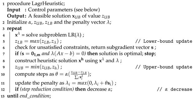In the pseudocode of Algorithm 1, step 4 solves the subproblem, obtaining a solution ${\mathbf{x}}^{\lambda }$ which is possibly infeasible for the whole problem but whose cost $z_{l}ambda$ is a lower bound to the problem’s optimal cost. Step 6 checks its feasibility and returns a vector s of subgradients, which is null in the case of a feasible solution. Step 7 is the optimality check and step 8 is the call to the fixing heuristic. Finally steps 10–11 implement the penalty update heuristic and step 12 implements Polyak’s rule [30] that ensures the convergence of the series of penalty vectors.

The specific problem we applied the Lagrangian heuristic to is the GAP. This problem asks to uniquely assign n clients, index set $J=\{1,\dots ,n\}$, to m servers, index set $I=\{1,\dots ,m\}$, so that a cost function gets minimized while satisfying capacity constraints. Assignment costs are specified by a cost matrix $\mathbf{C}={\left[c_{ij}\right]}_m^n$, server capacities by a vector $\mathbf{Q}={\left[Q_i\right]}_m$ and client requests to servers by a request matrix $\mathbf{q}={\left[q_{ij}\right]}_m^n$. Partial assignments are not allowed, thus the mathematical formulation of the GAP is as follows.

$$\begin{array}{cc}\hfill z_{GAP}=\mathbf{min}& \sum _{i\in I}\sum _{j\in J}{c}_{ij}{x}_{ij}\hfill \end{array}$$

(1)

$$\begin{array}{ccc}\hfill \mathbf{subject}\mathbf{to}& \sum _{j\in J}{q}_{ij}{x}_{ij}\le Q_i\hfill & \hfill i\in I\end{array}$$

(2)

$$\begin{array}{ccc}\hfill & \sum _{i\in I}{x}_{ij}=1\hfill & \hfill j\in J\end{array}$$

(3)

$$\begin{array}{ccc}\hfill & x_{ij}\in \{0,1\}\hfill & \hfill i\in I,j\in J\end{array}$$

(4)

It is possible to relax in a Lagrangian fashion either constraints (2) or constraints (3) (or both), thus obtaining two (three) different subproblems to solve at step 4.

Algorithm 1 when applied to the GAP has six parameters to set, which are:

• alphainit: initial $\alpha$ value for penalty updates;
• alphastep: step reduction (step 12);
• minalpha: minimum step length value (step 12);
• inneriter: internal iteration number before changing $alpha$ (step 12);
• maxiter: maximum number of iterations (terminating condition, step 13);
• algotype: which subproblem is used (step 4) (see [2] for details).

The GAP is a very well known and studied problem, and several benchmark instance sets exist. The online collection from which we downloaded our test set was the GAPLIB instance library [31], which contains most instances from the literature.

3.2. Robust Tabu Search and the QAP

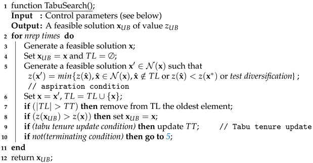
Tabu search is a very well-known metaheuristic, originally proposed in [32,33], that basically extends a local search by forcing a move to the best neighbor solution at each iteration, even if it is worse than the incumbent one. To avoid cycling, a memory structure is used that keeps track of the last explored solutions, or abstractions thereof, and forbids going back to them by declaring them “tabu”. The number of iterations when an element is considered tabu, corresponding to the length of the tabu list, is also called the “tenure” of the tabu elements. Several details in the algorithm can be varied, giving rise to a rich specific literature [34]. We used a specific variant called robust tabu search [4] which, despite its simplicity, proved to be effective on the QAP. The pseudocode is presented as Algorithm 2. The label robust was given because it “requires less complexity and fewer parameters than earlier adaptations”, further specifying that it “has a minimum number of parameters and is (…) capable of obtaining solutions comparable to the best previously found without requiring (…) altered parameter values” [4]. This focus on parameter independence makes this algorithm particularly well suited for validating our approach to individualized settings.

Two specific elements make this version of tabu search robust. The first is that the tenure of the tabu items is a random variable instead of a static value. A maximum and minimum tenure is given, and a value is generated iteratively within that interval.

The second feature is a long-term diversification method that favors moves that have not been performed for a long time. If a move has not been tested for a long number of iterations, the move is executed regardless of its quality. This is included in an “aspiration” test, which otherwise dictates that if a move generates a solution better than any previous one, it will be executed even if it is tabu.

Algorithm 2: Robust Tabu Search

The heuristic was applied to the QAP, whose formulation can be described as follows. We are given an index set F of n facilities to be assigned to an index set L of n locations. Let $\mathbf{D}={\left[d_{ih}\right]}_n^n$ be the distance matrix from each location $i\in L$ to each location $h\in L$, and let $\mathbf{F}={\left[f_{jk}\right]}_n^n$ be the expected flow from facility $j\in F$ to facility $k\in F$. Finally, let $c_{ik}$ be a fixed cost for assigning facility k to location i, for each $i\in L$ and $k\in F$. By using binary variables $x_{ik}$ = 1 iff facility k is assigned to location i, the QAP can be stated as the following quadratic 0-1 problem:

$$\begin{array}{cc}\hfill z_{QAP}=\mathbf{min}& \sum _{i\in L}\sum _{j\in F}\sum _{h\in L}\sum _{k\in F}{d}_{ih}{f}_{jk}{x}_{ij}{x}_{hk}+\sum _{i\in L}\sum _{k\in F}{c}_{ik}{x}_{ik}\hfill \end{array}$$

(5)

$$\begin{array}{ccc}\hfill \mathbf{subject}\mathbf{to}& \sum _{i\in L}{x}_{ik}=1\hfill & \hfill k\in F\end{array}$$

(6)

$$\begin{array}{ccc}\hfill & \sum _{k\in F}{x}_{ik}=1\hfill & \hfill i\in L\end{array}$$

(7)

$$\begin{array}{ccc}\hfill & x_{ik}\in \{0,1\}\hfill & \hfill i\in L,k\in F\end{array}$$

(8)

Considering all possible hyperparameter choices actually embedded in the downloaded code, the robust tabu search was run with 7 parameters to set, which were:

• maxcpu, maximum total CPU allowed time (terminating condition, step 10);
• maxiter, maximum number of iterations (terminating condition, step 10);
• iter2resize, number of iterations before resizing the tabu list (step 9);
• minTLlength, minimum tabu list length (step 9);
• maxTLlength, maximum tabu list length (step 9);
• iter2aspiration, number of iterations before unconditional acceptance (test diversification, step 5);
• nrep, number of search restarts (step 2).

The QAP is a well-known and studied problem; there is an online repository, the QAPLIB library [35], which has collected most of the instances from the literature over the years. We downloaded our test set from that site.

4. Learning Configurations

Both formulations, GAP and QAP, assume that the instances are described by matrices of coefficients, two 2D matrices and a 1D vector in the case of GAP and three 2D matrices in the case of QAP. The use of a single data repository for the GAP and a single one for the QAP allowed us to take advantage of a common format for each of the two problems and, more importantly, to know exactly how each subset of instances contained in the repositories was generated. We had access to the underlying structural characteristics that led to the input data, and we were able both to generate new instances structured according to the repository instances and to design generative procedures that produced structures very different from those that appear in the literature instances. In the following subsections, we first describe how we obtained the learning examples to present to the neural network from the matrices and then, for each algorithm, how we constructed the corresponding training/validation/test sets.

4.1. Feature Selection

To abstract the details of each instance and to make instances with different dimensions compatible with a same learner, we used sets of descriptive statistics computed on each matrix, the same statistics for all matrices. We also computed sets of correlation statistics between matrices. The descriptive statistics included basic ones such as mean, standard deviation, IQR, etc., but also distribution fits for uniform (chi-square, Kolmogorov–Smirnov), for normal (chi-square, Shapiro–Wilk, Kolmogorov–Smirnov, Anderson–Darling), and for gamma (chi-square, Kolmogorov–Smirnov) distributions. Correlations quantified the average request vs. average capacity, cost/request correlation, etc. We are aware of contributions that have identified particularly significant complexity predictors for specific problems, such as ruggedness and flow dominance for the QAP [36], but we wanted to present here a general methodology that can be applied to any combinatorial optimization problem of interest, so we computed the same statistics on all matrices, regardless of the problem they referred to.

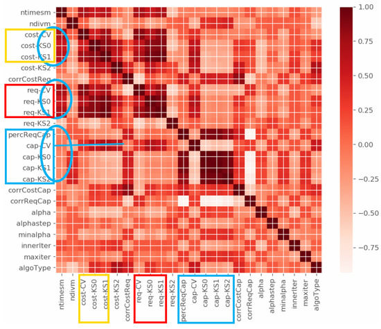
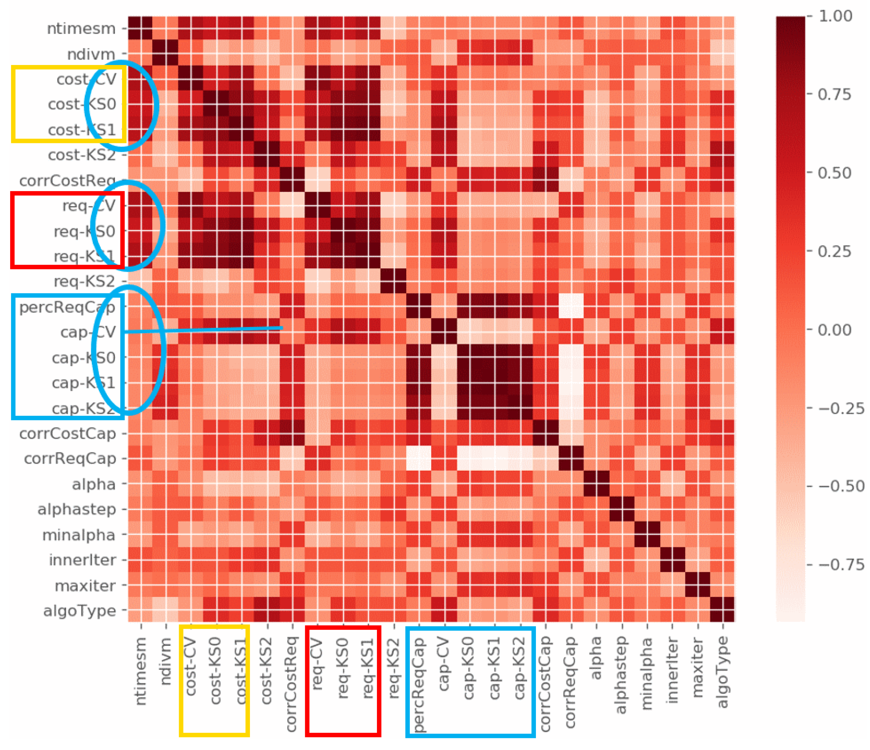
This resulted in about 100 different statistics for each instance in the case of the QAP and about 70 in the case of the GAP, which were preprocessed for relevance and only the surviving ones were to be used as input for the learning module. Data filtering was done first by removing all statistics that varied too little over the training set (low variance filter), then we ran a PCA which suggested that 7 variables could account for more than 97% of the variance, both in the case of the GAP and QAP, but we could not use the principal components as we wanted to keep the original statistics. However, following the decreasing relevance order and the analysis of the heat map of the correlations between the variables, we were able to shortlist the set and reduce it to 11 variables in the case of the GAP and 14 in the case of the QAP. Figure 1 shows the heat map of surviving descriptive statistics for the case of the Lagrangian heuristic; blue balloons outline the subsets of highly correlated variables that were eventually represented by a single variable of each subset.

Figure 1. Descriptive statistics correlation, heat map.

4.2. Learning Lagrangian Heuristic Setting

All instances from the GAPLIB repository were generated under controlled settings and already separated into subsets of structurally similar instances. The main benchmarks from the literature, both included in the GAPLIB, are Yagiura’s [37] and Beasley’s OR-library [38]. Both authors generated instances that were supposed to range from easy to difficult. We independently optimized the parameter setting on 4 different subsets, 2 derived from the biggest OR-library instances (sets 11 and 12) and 2 consisting of the hardest Yagiura instances (sets D and E) by means of the automatic configurator irace [12]. The other sets from these literature benchmarks were composed of instances too easy to solve and would have biased the parameter choice toward values of little interest for more complex tasks.

Beasley’s OR-library instances were generated with costs $c_{ij}$ as integers from the uniform distribution U(15, 25), requests $q_{ij}$ from uniform distribution U(5, 25), and capacities were computed as $b_i$ = $0.8{\sum }_{j\in J}{q}_{ij}/m$. Set 11 had $m=10$ and $n=50$ ($r=n/m=5$) while set 12 had $m=10$ and $n=60$ ($r=n/m=6$).

Yagiura’s instances of type D had requests $q_{ij}$ from uniform distribution U[1, 100], costs computed as $c_{ij}$ = $111-q_{ij}+e_1$, where $e_1$ is from uniform distribution U[−10, 10] and $b_i$ = $0.8{\sum }_{j\in J}{q}_{ij}/m$. Type E instances had requests $q_{ij}$ = $1-10ln$$e_2$, with $e_2$ from uniform distribution U(0, 1], costs $c_{ij}=1000/a_{ij}-10e_3$, with $e_3$ from uniform distribution U[0, 1] and capacities $b_i=0.8{\sum }_{j\in J}{q}_{ij}/m$.

This detailed knowledge of the generation procedure allowed us to generate additional instances that were structurally similar to the benchmark ones.

4.2.1. Data Augmentation

The chosen benchmark sets consisted of a total of 31 instances, which were too few for effective generalization. However, we were able to extend the training dataset without losing the knowledge of the instance structures. The data augmentation resulted from two contributions.

The first augmentation stemmed from the observation that learning in our system used a feature that distinguished it from standard supervised learning. Typically, learning is implemented by defining a training set, possibly a validation set, and then a test set. It is assumed that the input–output pairs presented with the training set are learned as shown, and that the network works as much as possible as an associative memory on them, reproducing the output when the training input is re-presented. In our case, we were much more interested in supporting abstraction and generalization, and we did this also by means of a feature offered by irace. This configurator proposes, for each set of instances on which parameters are optimized, up to 4 best settings it can find. We used them all in the training set, which was therefore composed of records that associated the same input to different outputs, making it impossible for the network to reproduce exactly the training set after learning. We experimentally noticed that including all suggested settings in the training set permitted a more effective generalization than generating only a record from the best one. This resulted in 77 records derived from the automatic configurator.

However, that set was still a small one, so we artificially enlarged it. This was possible because the authors described the generators used for producing the instances of the subsets, along with the parameter values they used. We reimplemented the generators and obtained 28 further instances similar to the examples used by the configurators, and we associated each of them with the best parameter configurations obtained for the published instances. The final complete training composed by literature-related instances set consisted of 105 records.

4.2.2. Neural Learning

Finally, the subset of relevant statistics was separately related to each parameter to be set, in order to determine which of the statistics were relevant to each parameter. This allowed us to reduce the search space because we could compute further correlations with respect to each specific output.

The final parameter settings were generated by neural networks, specifically feed-forward MLPs. The network input consisted of arrays containing the selected statistical values computed on each instance, and the output was the corresponding parameter value. The networks, all composed of 3 dense layers, had the structure reported below, where for each parameter, we detail the number of input neurons, the number of hidden neurons, and the number of output neurons (always one, since each network is tailored to one parameter) of the corresponding network. The activation function was a sigmoid for the hidden layer and a ReLU for the output layer. The number of hidden neurons was determined by checking the effectiveness of all values in the interval $[n/2,2n]$, where n is the number of input neurons, and keeping the best one, the smallest in case of ties. Comparable results were also obtained with n-4-4-1 architectures, which were discarded because they required more connections.

• alphainit: 5-10-1 network (71 weights);
• alphastep: 7-7-1 network (64 weights);
• minalpha: 8-5-1 network (51 weights);
• inneriter: 5-10-1 network (71 weights);
• maxiter: 6-4-1 network (33 weights);
• algotype: 8-7-1 network (71 weights).

In the case of the GAP, network learning could also have been modeled as a multivalued, multioutput regression with 11 inputs and 6 outputs. However, given the limited size of the training set and the limited correlation among parameter values, the resulted search was more effective when optimizing a specific network for each parameter as described.

4.3. Learning Tabu Search’s Heuristic Setting

The structure of the experiment for the QAP was the same as for the GAP. The QAP has more diverse instance sets, often derived from real-world applications, and QAP instances can be very challenging, even at relatively small dimensions. Therefore, for our tests, we removed the instances that were too small, which would be too easy to solve anyway, and those that were too large, which would require a long CPU time to optimize. Furthermore, we also removed the instances from the sets that, after the above selection, were left with too few items and those for which we were uncertain about the generation procedure. The available QAPLIB benchmark sets that met these requirements consisted all of midsized instances (n between 12 and 50) of the sets BUR, CHR, ESC, HAD, LIPA, NUG, and TAI. Collectively, they amounted to 85 instances that, after the inclusion of the best configuration for each group proposes by irace (up to 4), generated a training set of 305 records.

In that case, there was no need for data augmentation because we considered the dataset to be of sufficient size. However, even in that case, we independently optimized an MLP network for each of the control parameters, according to what we did in the GAP case. We separately optimized the tabu search control parameters on each of these sets using irace. The number of hidden neurons was determined as for GAP, resulting in the following architectures.

• maxiter: 5-4-1 network (29 weights);
• minTLlength: 6-8-1 network (65 weights);
• maxTLlength: 6-7-1 network (57 weights);
• iter2aspiration: 5-9-1 network (64 weights);
• iter2resize: 7-5-1 network (46 weights);
• maxcpu: 6-7-1 network (57 weights);
• nrep: 7-8-1 network (73 weights).

5. Computational Results

All computational tests were conducted on a Windows 10 machine with 16 GB of RAM, and all computations were performed on a single CPU, in a single thread. Notwithstanding that MLP backpropagation-based learning is a standard procedure, network training was tested on four different frameworks based on four different languages to verify this assumption. The frameworks were: accord.net (C#) [39], ANNT (C++) [40], tensorflow (python) [41], and nnet (caret) (R) [42]. The efficiency and effectiveness were indeed comparable between all frameworks, possibly because the learning task was very simple, so a few seconds of CPU time were sufficient to achieve the final good performance in all cases. In the following, results were produced by the python/tensorflow implementation. We remark that the training time was incurred only once per algorithm per problem, so each new instance did not incur any additional training time for its solution.

5.1. In-Sample Validation

A first set of tests verified whether individualized settings improved over problem-wide ones on the training set. To this end, a base setting $S_0$ was obtained by running irace on a subset of 20 instances, uniformly chosen among all instance subsets, first for the GAP, then for the QAP. Each instance of the test set was optimized either by LagrHeu or by a tabu search, both with the $S_0$ setting and with the $S_n$ setting suggested by the network. Finally, for each problem, we computed how many times $S_0$ or $S_n$ was better. A configuration was considered better than another on a given instance if it produced a better solution, or if it produced a solution of the same quality as its counterpart but in less CPU time. When solution quality was equal and cpu times differed by less than 10%, $S_0$ was considered better, breaking ties in favor of the null hypothesis. While a simple numerical comparison could determine relative performance, a statistical significance test based on the binomial distribution was used to assess the significance of the difference, with hypothesis H0 assuming that all differences were due to chance alone ($p=0.5$). Note that the results reported in the $S_0$ column correspond to the results obtained by irace alone; therefore, the table shows a comparison of the results obtained by the individualized settings against those obtained with a state-of-the-art automatic configurator.

We did not report the CPU times needed for obtaining the individualized settings because they corresponded to the time needed to propagate the input in a small three-level MLP, therefore less than 1 ms.

In the case of the GAP, the in-sample validation produced the results shown in Table 1. The individualized setting produced more dominating results on all instance subsets, although statistical significance ($\alpha =0.05$) was never reached, albeit close for the Yagiura E subset, possibly because it counted a larger number of instances.

Table 1. GAP, in-sample validation.

Type	n	${\mathit{S}}_0$	${\mathit{S}}_{\mathit{n}}$	p (Binomial)
Beasley 11	5	1	4	0.188
Beasley 12	5	2	3	0.500
Yagiura D	6	2	4	0.344
Yagiura E	13	4	11	0.059

In the case of the QAP, the in-sample validation reported in Table 2 was, as expected, less conclusive, as can be seen from the higher values of the binomial probabilities. Although the individualized setting produced dominating results in almost all rows, statistical significance was again never reached. This is not surprising, since the robust tabu search was explicitly designed to be insensitive to the parameter setting, so tuning it should not have much effect. Another possible reason for the failure to reach significance is the low numerosity of the instance sets. Given these obstacles, the consistently higher number of better results obtained with individualized settings is noteworthy. Note that the Lagrangian heuristic is deterministic, while the robust tabu search has a random component, so the results in Table 2 are six-run averages. However, it is worth noting that the robust tabu search proved to be very stable in its results, in most cases producing identical results in all repetitions.

Table 2. QAP, in-sample validation.

Type	n	${\mathit{S}}_0$	${\mathit{S}}_{\mathit{n}}$	p (Binomial)
BUR	8	3	5	0.363
CHR	14	4	10	0.090
ESC	18	8	10	0.407
HAD	5	3	2	0.813
LIPA	6	2	4	0.344
NUG	13	4	9	0.133
TAI	17	5	12	0.072

5.2. Out-of-Sample Validation

In out-of-sample tests, the optimized problemwide setting and the neural-suggested setting were applied to instances not used by irace in the optimization phase. This was done in two steps, first using the full datasets from the literature and then augmenting them with newly generated benchmarks.

5.2.1. Full Datasets

In the first step, a test set was used for the GAP that included all literature instances of the chosen subsets, not just a sample of them, although the simplest sets were quickly solved to optimality in all cases. Each instance was solved with both the global setting and the individualized setting. The results are given in Table 3 and are consistent with those of Table 1. We can see that the significance was slightly improved, mainly due to the increased cardinalities, but the relative performance was basically the same. The comparatively higher number of instances better solved by the global setting was mainly due to the fact that the tie-breaking policy acted on instances that were quickly solved to optimality.

Table 3. GAP, full literature test sets.

Type	n	${\mathit{S}}_0$	${\mathit{S}}_{\mathit{n}}$	p (Binomial)
Beasley	60	23	37	0.046
Yagiura	39	14	25	0.054

Similarly, we constructed a test set including all QAPLIB instances with n between 12 and 50. This resulted in the inclusion of the sets ELS (one instance), KRA (three instances), ROU (three instances), SCR (three instances), SKO (two instances), STE (three instances), THO (two instances), and WIL (one instance). This brought the total number of instances to 103 but the added sets being so small, we present in Table 4 the results grouped by size rather than by name.

Table 4. QAP, full literature test sets.

Size	n	${\mathit{S}}_0$	${\mathit{S}}_{\mathit{n}}$	p (Binomial)
12–15	19	11	8	0.820
16–20	31	14	17	0.360
21–30	27	9	18	0.061
31–40	19	7	12	0.180
41–50	7	2	5	0.227

The results of Table 4 were consistent with those of Table 2 in that individualized settings outperformed global settings in all but one row, without reaching statistical significance. The only subset where global settings performed better, modulo the tie-breaking policy, was that of the simplest instances, where both codes could quickly solve all instances.

5.2.2. New Instances

In order to better evaluate the abstraction power of the neural adaptation, we generated some new instances either according to the literature generators or based on data distributions that were clearly different from the literature ones. In particular, since we had to generate data matrices for both problems, we generated them according to a gamma distribution, which is both very flexible and possibly very different from the uniform distribution that is usually at the core of the generation of the literature benchmarks.

In the case of the GAP, we generated 15 instances structurally similar to Beasley’s OR-library ones, 18 similar to Yagiura’s E ones, and 30 instances based on the gamma distribution. The literature-like instances were generated in order to achieve a clearer significance, while the gamma ones were to assess the abstraction power of the trained networks. All instances are available from [31] and validation results are reported in Table 5.

Table 5. GAP, generated instances.

Type	n	${\mathit{S}}_0$	${\mathit{S}}_{\mathit{n}}$	p (Binomial)
Beasley-like	15	4	11	0.059
Yagiura-like	18	5	13	0.048
gamma	30	7	23	0.003

The table shows that the number of instances better solved with the individualized settings was higher than with the global setting in all rows. In this case, statistical significance at $\alpha =0.05$ was reached for two subsets, the Yagiura-like and the newly generated gamma. The results for the Yagiura were consistent with those of Table 5, which already bordered significance, but in that case, from the nonsignificance side. The results on the gamma instances confirmed that a setting optimized for a subset of the instance space can be suboptimal when applied to instances from a different subset, and that neural abstraction can help to constrain the problem. Indeed, we see that the significance of the difference was greatly increased on these instances, and we interpreted this result as consistent with the assumption that motivated the generation of these instances, i.e., that a setting optimized for a given instance set can be suboptimal when applied to instances that are structurally very different from those on which it was optimized.

Finally, we also generated instances for the QAP, both replicating the generation procedure for the subsets where it was reproducible (i.e., the CHR, NUG, and TAI subsets) and using the gamma generator to generate the QAP matrices. The results are shown in Table 6. Again, compared to the results of their GAP counterpart in Table 5, these results outlined a smaller impact of the individualized approach, and this testified to the robustness of the robust tabu search, i.e., the low sensitivity to parameters as indicated by the name of the method. However, even in that case, the highest significance was achieved on the new gamma instances. This was consistent with the results presented in Table 5, where the gamma instances also had a greater significance. We thus have further confirmation that unexplored instance subspaces can limit the effectiveness of settings optimized elsewhere in the instance space, and that the MLP abstraction can help mitigate this problem, possibly biasing the setting in a direction related to the properties of the vector of statistics of structural properties.

Table 6. QAP, generated instances.

Type	n	${\mathit{S}}_0$	${\mathit{S}}_{\mathit{n}}$	p (Binomial)
CHR-like	15	5	10	0.151
NUG-like	15	6	9	0.304
TAI-like	15	5	10	0.151
gamma	30	11	19	0.100

6. Conclusions

This work reported on results obtained by exploiting the abstraction capabilities of neural networks, in particular multilayer perceptrons, when attempting to identify optimized instance-level parameter settings for an algorithm of interest applied to a given problem. Our proposal did not cover adaptive parameter optimization or algorithm portfolio selection, but it is a contribution to the relatively unexplored area of instance-level continuous parameter optimization.

We proposed a generic pipeline from feature identification through feature selection, possibly data augmentation, and neural learning, where standard supervised learning was adapted to favor abstraction over precision. Computational results on different algorithms and different problems confirmed the effectiveness of the method.

Future work includes a quantitative analysis of the improvement in solution quality that can be achieved by individualized settings. In this paper, we committed to using codes from the literature, codes that were unaware of our target use. This entailed the problems to which they were applied and resulted in differences in solution quality between global and individualized settings usually well below 5%, a position that did not change much using larger instances. An analysis of codes and problems that allows for larger differences in solution quality due to different settings can take this research beyond the analysis of rankings presented in this work.

References

- Wolpert, D.; Macready, W. No Free Lunch Theorems for Optimization. IEEE Trans. Evol. Comput. 1997, 1, 67–82. [Google Scholar] [CrossRef] [Scilit]
- Boschetti, M.A.; Maniezzo, V. Benders decomposition, Lagrangean relaxation and metaheuristic design. J. Heuristics 2009, 15, 283–312. [Google Scholar] [CrossRef] [Scilit]
- Maniezzo, V.; Boschetti, M.; Stützle, T. Matheuristics; EURO Advanced Tutorials on Operational Research; Springer International Publishing: New York, NY, USA, 2021. [Google Scholar]
- Taillard, E. Robust taboo search for the quadratic assignment problem. Parallel Comput. 1991, 17, 443–455. [Google Scholar] [CrossRef] [Scilit]
- Aleti, A.; Moser, I. A Systematic Literature Review of Adaptive Parameter Control Methods for Evolutionary Algorithms. ACM Comput. Surv. 2016, 49, 1–35. [Google Scholar] [CrossRef] [Scilit]
- Kerschke, P.; Hoos, H.; Neumann, F.; Trautmann, H. Automated Algorithm Selection: Survey and Perspectives. Evol. Comput. 2018, 27, 1–47. [Google Scholar] [CrossRef] [Scilit] [PubMed]
- Talbi, E.G. Machine Learning into Metaheuristics: A Survey and Taxonomy. ACM Comput. Surv. 2021, 54, 1–32. [Google Scholar] [CrossRef] [Scilit]
- Bartz-Beielstein; Flasch, O.; Koch, P.; Konen, W. SPOT: A Toolbox for Interactive and Automatic Tuning in the proglangR Environment. In Proceedings 20. Workshop Computational Intelligence; KIT Scientific Publishing: Karlsruhe, Germany, 2010. [Google Scholar]
- Birattari, M.; Stützle, T.; Paquete, L.; Varrentrapp, K. A Racing Algorithm for Configuring Metaheuristics. In Proceedings of the GECCO 2002, New York, NY, USA, 9–13 July 2002; Langdon, W., Cantú-Paz, E., Mathias, K., Roy, R., Davis, D., Poli, R., Balakrishnan, K., Honavar, V., Rudolph, G., Wegener, J., et al., Eds.; Morgan Kaufmann Publishers: San Francisco, CA, USA, 2002; pp. 11–18. [Google Scholar]
- Hutter, F.; Hoos, H.; Leyton-Brown, K. Automated Configuration of Mixed Integer Programming Solvers. In Proceedings of the CPAIOR 2010, Bologna, Italy, 14–18 June 2010; Lodi, A., Milano, M., Toth, P., Eds.; Lecture Notes in Computer Science. Springer: New York, NY, USA, 2012; Volume 6140, pp. 186–202. [Google Scholar]
- Hutter, F.; Hoos, H.H.; Leyton-Brown, K.; Stützle, T. ParamILS: An Automatic Algorithm Configuration Framework. J. Artif. Intell. Res. 2009, 36, 267–306. [Google Scholar] [CrossRef] [Scilit]
- López-Ibáñez, M.; Dubois-Lacoste, J.; Pérez Cáceres, L.; Birattari, M.; Stützle, T. The irace package: Iterated racing for automatic algorithm configuration. Oper. Res. Perspect. 2016, 3, 43–58. [Google Scholar] [CrossRef] [Scilit]
- Bacanin, N.; Bezdan, T.; Tuba, E.; Strumberger, I.; Tuba, M. Optimizing Convolutional Neural Network Hyperparameters by Enhanced Swarm Intelligence Metaheuristics. Algorithms 2020, 13, 67. [Google Scholar] [CrossRef] [Scilit]
- Filippou, K.; Aifantis, G.; Papakostas, G.; Tsekouras, G. Structure Learning and Hyperparameter Optimization Using an Automated Machine Learning (AutoML) Pipeline. Information 2023, 14, 232. [Google Scholar] [CrossRef] [Scilit]
- Esmaeili, Z.A.; Ghorrati, E.T.M. Agent-Based Collaborative Random Search for Hyperparameter Tuning and Global Function Optimization. Systems 2023, 11, 228. [Google Scholar] [CrossRef] [Scilit]
- Birattari, M.; Yuan, Z.; Balaprakash, P.; Stützle, T. F-Race and Iterated F-Race: An Overview. In Experimental Methods for the Analysis of Optimization Algorithms; Bartz-Beielstein, T., Chiarandini, M., Paquete, L., Preuss, M., Eds.; Springer: Berlin/Heidelberg, Germany, 2010; pp. 311–336. [Google Scholar]
- Rechenberg, I. Evolutionsstrategie—Optimierung Technischer Systeme Nach Prinzipien der Biologischen Evolution; Frommann-Holzboog-Verlag: Stuttgart, Germany, 1973. [Google Scholar]
- Beyer, H.G.; Schwefel, H.P. Evolution Strategies—A Comprehensive Introduction. Nat. Comput. 2002, 1, 3–52. [Google Scholar] [CrossRef] [Scilit]
- Rice, J.R. The Algorithm Selection Problem. Adv. Comput. 1976, 15, 65–118. [Google Scholar]
- Xu, L.; Hutter, F.; Hoos, H.; Leyton-Brown, K. SATzilla2009: An Automatic Algorithm Portfolio for SAT. 2009. Available online: https://www.cs.ubc.ca/~hutter/papers/09-SATzilla-solver-description.pdf (accessed on 4 May 2023).
- Kerschke, P.; Kotthoff, L.; Bossek, J.; Hoos, H.H.; Trautmann, H. Leveraging TSP Solver Complementarity through Machine Learning. Evol. Comput. 2017, 26, 597–620. [Google Scholar] [CrossRef] [Scilit] [PubMed]
- Xu, L.; Hoos, H.; Leyton-Brown, K. Hydra: Automatically Configuring Algorithms for Portfolio-Based Selection. Proc. AAAI Conf. Artif. Intell. 2010, 24, 210–216. [Google Scholar] [CrossRef] [Scilit]
- Kotthoff, L. LLAMA: Leveraging Learning to Automatically Manage Algorithms. arXiv 2013. [Google Scholar] [CrossRef] [Scilit]
- Smith-Miles, K.; Muñoz, M.A. Instance Space Analysis for Algorithm Testing: Methodology and Software Tools. ACM Comput. Surv. 2023, 55, 1–31. [Google Scholar] [CrossRef] [Scilit]
- Kadioglu, S.; Malitsky, Y.; Sellmann, M.; Tierney, K. ISAC—Instance-Specific Algorithm Configuration. Front. Artif. Intell. Appl. 2010, 215, 751–756. [Google Scholar]
- Dobslaw, F. A Parameter Tuning Framework for Metaheuristics Based on Design of Experiments and Artificial Neural Networks; World Academy of Science, Engineering and Technology: Istanbul, Turkey, 2010; Volume 64. [Google Scholar]
- Maniezzo, V. LagrHeu Public Code. Web Page. 2018. Available online: https://github.com/maniezzo/LagrHeu (accessed on 9 February 2023).
- Taillard, E. Éric Taillard Public Codes. Web Page. 1991. Available online: http://mistic.heig-vd.ch/taillard/ (accessed on 9 February 2023).
- Shor, N.Z. Minimization Methods for Non-Differentiable Functions; Springer: Berlin/Heidelberg, Germany, 1985. [Google Scholar]
- Polyak, B.T. Minimization of Unsmooth functionals. USSR Comput. Math. Math. Phys. 1969, 9, 14–29. [Google Scholar] [CrossRef] [Scilit]
- Maniezzo, V. GAPlib: Bridging the GAP. Some Generalized Assignment Problem Instances. Web Page. 2019. Available online: http://astarte.csr.unibo.it/gapdata/GAPinstances.html (accessed on 9 February 2023).
- Glover, F. Tabu Search—Part I. ORSA J. Comput. 1989, 1, 190–206. [Google Scholar] [CrossRef] [Scilit]
- Glover, F. Tabu Search—Part II. ORSA J. Comput. 1990, 2, 14–32. [Google Scholar] [CrossRef] [Scilit]
- Glover, F.; Laguna, M. Tabu Search; Kluwer Academic Publishers: Dordrecht, The Netherlands, 1997. [Google Scholar]
- Burkard, R.; Çela, E.; Karisch, S.E.; Rendl, F.; Anjos, M.; Hahn, P. QAPLIB—A Quadratic Assignment Problem Library—Problem Instances and Solutions. Web Page. 2022. Available online: https://datashare.ed.ac.uk/handle/10283/4390 (accessed on 9 February 2023).
- Angel, E.; Zissimopoulos, V. On the Hardness of the Quadratic Assignment Problem with Metaheuristics. J. Heuristics 2002, 8, 399–414. [Google Scholar] [CrossRef] [Scilit]
- Yagiura, M. GAP (Generalized Assignment Problem) Instances. Web Page. 2006. Available online: https://www-or.amp.i.kyoto-u.ac.jp/members/yagiura/gap/ (accessed on 9 February 2023).
- Cattrysse, D.; Salomon, M.; Van Wassenhove, L.N. A set partitioning heuristic for the generalized assignment problem. Eur. J. Oper. Res. 1994, 72, 167–174. [Google Scholar] [CrossRef] [Scilit]
- Accord.net. Web Page. Available online: http://accord-framework.net/ (accessed on 9 February 2023).
- ANNT. Web Page. Available online: https://github.com/cvsandbox/ANNT (accessed on 9 February 2023).
- Tensorflow. Web Page. Available online: https://www.tensorflow.org/ (accessed on 9 February 2023).
- Nnet (caret). Web Page. Available online: https://cran.r-project.org/web/packages/nnet (accessed on 9 February 2023).
Disclaimer/Publisher’s Note: The statements, opinions and data contained in all publications are solely those of the individual author(s) and contributor(s) and not of MDPI and/or the editor(s). MDPI and/or the editor(s) disclaim responsibility for any injury to people or property resulting from any ideas, methods, instructions or products referred to in the content. |
© 2023 by the authors. Licensee MDPI, Basel, Switzerland. This article is an open access article distributed under the terms and conditions of the Creative Commons Attribution (CC BY) license (https://creativecommons.org/licenses/by/4.0/).