


Abstract
Accurate time-domain photovoltaic (PV) models are needed to evaluate performance under outdoor variability beyond STC datasheet conditions. This paper presents a traceable modeling workflow based on the standard single-diode formulation, implemented in MATLAB/Simulink (R2023a) as a modular white-box architecture that explicitly resolves photocurrent generation and loss mechanisms (diode recombination, shunt leakage, and series resistance effects) with temperature-consistent propagation through and saturation-current terms. The method couples optical boundary conditions to the electrical model by embedding plane-of-array (POA) excitation via the incidence angle and roof albedo directly into the photocurrent source term, preserving the causal chain from mounting geometry to electrical response. Calibration is separated from prediction by initializing key parameters using the standard Simulink PV block and then freezing them for time-domain evaluation. The workflow is validated on a 395 W rooftop prototype using 1 min resolved POA irradiance (ISO 9060:2018 Class A radiometric chain) and module temperature (IEC 60751 Class A Pt100), synchronized with electrical measurements. Over a multi-week campaign, the model exhibits high fidelity, with a worst-case relative current error of ~1.1% and a consistently low bias and dispersion, quantified by ME, MAE, RMSE, , and thresholded MAPE.
1. Introduction
Rising carbon emissions are widely regarded as one of the defining environmental challenges of the twenty-first century. The dominant contributor is the combustion of fossil fuels, coal, oil, and natural gas, which still underpin most energy supply and account for roughly 70% of global carbon emissions [1,2]. Sustained emissions increase the atmospheric concentration of greenhouse gases, intensifying heat retention and driving a rapid rise in average global temperatures. This acceleration of global warming is amplifying climate-related risks and increasing the vulnerability of natural and human systems worldwide [3,4,5,6].
To address the environmental impacts and resource limitations linked to fossil fuel-based energy, numerous renewable options have been pursued [7,8,9,10]. Within this portfolio, solar energy stands out due to its wide availability and substantial resource potential [11,12,13]. Solar conversion is commonly grouped into two main approaches: solar–thermal (photothermal) and photovoltaic (PV). PV systems are particularly attractive because they convert sunlight directly into electricity [14] without local emissions, supporting clean and sustainable power generation with low operating costs after installation [8,15]. However, PV output is inherently variable and intermittent, as it depends on rapidly changing atmospheric conditions [16,17]. This variability introduces operational and planning difficulties when PV penetration increases in power systems. Accordingly, PV power forecasting has become an important tool for improving grid reliability [18] and security under high PV integration, supporting tasks such as scheduling and dispatch, storage coordination, automatic generation control, and the allocation of operating reserves [19].
Over the past few years, solar photovoltaic (PV) deployment has expanded rapidly worldwide: the cumulative installed capacity rose from about 480 GW in 2018 to more than 1.6 TW by 2023 [20]. This upward trajectory is widely expected to persist, with many outlooks projecting a PV capacity on the order of ~2.8 TW by 2030 and ~8.5 TW by 2050. From an end-user perspective, PV investments are typically driven by two core goals: exporting electricity for revenue or lowering on-site electricity expenditures through self-consumption [21]. The expanding deployment of solar-based electricity generation has become a key driver of the decarbonization progress observed in recent years [22,23].
Because a PV system’s core function is to transform incident solar radiation into electricity, improving its conversion efficiency has become a central research focus [24]. Compared with other renewable technologies, photovoltaic generation is often associated with the lowest levelized cost of electricity [25,26]. For fixed irradiance and cell temperature, a PV array exhibits a unique operating point at which output power is maximized, known as the maximum power point (MPP), located at the peak of the array’s power–voltage (P-V) curve [27,28]; this peak shifts as irradiance and temperature change [29]. In practical installations, arrays are also often subject to partial shading from nearby obstacles such as trees or buildings, creating partial shading conditions (PSCs) [30,31]. Under PSCs, the P-V characteristic becomes multi-peaked, producing several local maxima (LMPPs) and a single global maximum (GMPP) [32]. Since ambient conditions can vary quickly, keeping the array operating at the true power-optimal voltage/current is nontrivial [33]. Therefore, maximum power point tracking (MPPT) methods, implemented in PV power-conditioning and control hardware, are employed to continually identify and enforce the optimal operating point [34,35,36].
In this study, we address the gap between STC-anchored PV characterization and the requirements of time-domain model validation under real outdoor variability by developing a traceable plane-of-array (POA) to electrical-output workflow implemented in MATLAB/Simulink (R2023a) and benchmarked against minute-resolved field measurements. The underlying electrical formulation adopts the well-established single-diode equivalent-circuit model; accordingly, the novelty of the present work does not lie in introducing new diode equations, but in their rigorous implementation, coupling to measured optical/thermal boundary conditions, and traceable time-domain validation. Starting from the single-diode equivalent circuit, we derive a physics-informed current balance in which the terminal current is explicitly decomposed into photogenerated excitation and loss mechanisms (diode recombination and shunt leakage), while parasitic resistances are retained to preserve fill-factor degradation and voltage drop effects.
A distinctive aspect of the proposed workflow is that the photogenerated current excitation is driven by tilted POA irradiance computed and applied at the measurement time-step, and it is augmented with incidence angle θ(t) and albedo Alb terms inside the excitation expression, thereby preserving the causal chain between mounting geometry, optical input, and electrical response. The incidence angle is computed at timestamp resolution using standard solar geometry relationships consistent with the fixed-tilt/fixed-azimuth mounting of the experimental module, and albedo is treated as an explicit optical modifier relevant to the roof surface context.
The model is realized as a modular “white-box” Simulink architecture, in which intermediate physical terms (, , , , ) are computed in dedicated subsystems rather than being embedded in a compact black-box solver. This implementation-oriented design enables numerical traceability (auditing of intermediate mechanisms) and reproducible verification beyond terminal I-V/P-V curve fitting. Furthermore, a calibration–prediction separation is enforced: key electrical parameters are initialized via the standard Simulink PV block under reference conditions, then frozen and propagated into the custom white-box implementation for time-domain evaluation. This methodological separation reduces solver-dependent equifinality and isolates the predictive performance of the coupled POA–electrical chain under real outdoor variability.
To ensure that simulations are representative and directly comparable to field behavior, the model is driven by experimentally acquired boundary conditions and evaluated as a pointwise mapping at a 1 min resolution. This design choice shifts the validation focus from steady-state curve reproduction to dynamic fidelity under irradiance ramps and cloud-induced disturbances, which are critical for PV sizing, performance assessment, and controller-coupled operation.
Experimental validation is conducted on a standalone prototype instrumented for the synchronized acquisition of electrical and environmental excitations. Tilted POA irradiance is measured using an ISO 9060:2018 Class A pyranometer (Hukseflux, Delft, The Netherlands) interfaced to a Campbell Scientific CR1000X datalogger (Campbell Scientific, Logan, UT, USA), ensuring deterministic scan/log timing and standards-bounded radiometric error sources; an additional PYR1307 pyranometer, ISO 9060:2018, Class C (Langlois, Gradignan Cedex, France) is deployed as an independent plausibility cross-check. Cell temperature is acquired with an IEC 60751 Class A Pt100 RTD (RS Components Ltd., Corby, Northants, UK) in a 4-wire Kelvin configuration and ratiometric measurement with excitation reversal, supporting traceable uncertainty budgeting and minimizing lead-wire and thermoelectric biases. The resulting dataset spans an extended campaign (2 August 2025–13 September 2025) over clear-sky and variable-cloud regimes, enabling the robust assessment of model consistency across a diverse excitation envelope.
2. Mathematical Modeling of PV Energy Conversion Systems
A photovoltaic cell can be regarded as a current generator and can be represented by the equivalent circuit shown in Figure 1. At the output terminals, the current originates from the light-generated current produced by the photovoltaic effect, modeled as an ideal current source. The terminal current is reduced by two main loss mechanisms: the diode current and the shunt (leakage) current that flows through the parallel resistance. Leakage typically appears due to localized imperfections in the p–n junction or unintended shunting paths, especially near the cell edges; these effects are lumped into the shunt resistance .
Figure 1.
Equivalent circuit configuration of a single-diode photovoltaic cell.
In addition, the series resistance accounts for the internal opposition to the flow of the generated current. Its magnitude is influenced by factors such as the p–n junction thickness, material impurities, and contact/interface resistances. An ideal photovoltaic cell would exhibit and . In practice, high-quality silicon cells commonly have in the range of 0.05–0.10 and around 300–400 kΩ. Small increases in can noticeably degrade conversion efficiency, whereas comparable variations in usually have a much weaker impact.
The fundamental equation for the single-diode equivalent-circuit model of a photovoltaic cell (Figure 1) is derived by applying Kirchhoff’s current law to the terminal current [37,38,39,40,41]:
where [37,38,39,40]
- denotes the output (delivered) current;
- represents the photocurrent produced in the cell by incident light (photocurrent/light-generated current);
- is the diode (recombination) current, which varies with the terminal voltage;
- is the leakage current flowing through the shunt path/resistance.
The cell photocurrent can be expressed as
where [38,39,40]
- denotes the short-circuit current, expressed as a temperature-dependent quantity;
- is the temperature coefficient associated with ;
- represents the photovoltaic cell temperature, in kelvin (K);
- is the reference temperature, in kelvin (K);
- is the incident solar irradiance, given in kW/.
To measure solar radiation in W/m2, we can rewrite Formula (2) as [42,43]
Another formula used to determine the light-generated current in the cell is [44]
where
- Alb is the albedo effective factor;
- θ is the angle of incidence of the solar radiation.
In Equation (4), the additive term is introduced as an effective rooftop ground-reflection augmentation rather than as the classical diffuse–isotropic ground-reflected irradiance contribution (Duffie & Beckman).
For comparison, conventional transposition theory models ground reflection as [44]
with (material ground albedo, –), (global horizontal irradiance, W·) and (tilt, °), where is the diffuse–isotropic ground view factor.
Our formulation deliberately departs from the diffuse–isotropic closure to accommodate roof-mounted near-field conditions in which the reflecting surface is (i) geometrically close, (ii) partially bounded, and (iii) potentially non-Lambertian, leading to reflected flux densities that can deviate from far-field isotropic predictions. Instead of explicitly modeling BRDF-driven anisotropy and view-factor complexity, the constant isotropic scaling (including the classical 1/2 factor) is embedded into , which is therefore interpreted as an installation-specific effective parameter rather than a purely material property. The modifier is used as a bounded geometric weight to capture incidence-dependent variability, increasing the relative influence of the effective reflection correction under high-incidence conditions (large ) when cosine projection reduces the beam contribution and reflected components may become comparatively more relevant on rooftop planes.
Compared to the Duffie–Beckman physics-based transposition approach, which is physically rigorous and explicitly geometry-driven via (tilt) and the surface azimuth, with strong optical–electrical separability and cross-site transferability when irradiance components are available (: direct normal irradiance; : diffuse horizontal irradiance; : global horizontal irradiance), yet reliant on robust component decomposition and a far-field diffuse–isotropic reflection premise that may be violated in rooftop near-field, non-Lambertian conditions, the effective augmentation in Equation (4) preserves an explicit geometric driver through (incidence angle) while operating directly on POA-level inputs and accommodating near-field directionality via a low-order, measurement-identifiable closure, at the expense of representing reflection through an installation-specific effective coefficient rather than a purely material albedo.
In solar energy applications, determining the solar geometry for tilted surfaces is essential, since such surfaces are representative of solar collectors regardless of their technology. These calculations are referenced to the horizontal plane and to the orientation relative to geographic south. The geometric parameters required for this evaluation are illustrated in Figure 2.
Figure 2.
Theoretical elements for solar geometry on tilted surfaces.
- [°] is the solar altitude angle;
- [°] is the solar azimuth angle;
- [°] is the orientation angle relative to the azimuth (relative to the south direction);
- [°] is the tilt angle relative to the horizontal.
The short-circuit current can be defined as a function of temperature as follows:
In the equivalent circuit of the single-diode model, ID is modeled using the Shockley equation for an ideal diode as follows [37,38,39,40,41]:
where
- n is the ideality factor of the diode, a unitless parameter, which for a single-junction cell typically ranges from 1 to 2;
- V is the cell voltage;
- Rs is the series resistance.
I0 is the saturation current given by the formula [38,40]
where
- Eg is the bandgap energy of the semiconductor material used in the solar cells.
IRS is the reverse saturation current given by the formula [40]
where
- Voc is the open-circuit voltage.
The open-circuit voltage can be defined as a function of temperature as follows:
where
- Kv is the temperature coefficient of the open-circuit voltage.
VT is the thermal voltage given by the formula [37,38,39,40,41]
where
- k, is Boltzmann’s constant (1.381 × 10⁻²³ J/K);
- q is the charge of the electron (1.6 × 10⁻¹⁹ C) [37,38].
Ish is the current lost due to the shunt resistance, given by the formula [37,38,39,40,41]
where
- Rsh is the shunt resistance.
Thus, the current supplied to the load is given by the following formula [37,38,39,40,41]:
If we use Equations (4) and (14), the current delivered to the load can be rewritten as
In typical solar cells, the leakage current Ish is usually very small compared to the other two currents in the equation, thus becoming negligible. Therefore, the saturation current of the diode can be experimentally determined by applying an open-circuit voltage Voc to a cell that is not exposed to light and measuring the current passing through it [37].
The fundamental relationship for electrical power in direct current (DC) can be expressed as
where represents the electrical power, is the electrical voltage, and is the electric current.
When several identical photovoltaic panels are connected in series, we denote by , the number of modules connected in series. In this configuration, the total voltage increases, and the resulting voltage is proportional to .
If the panels are connected in parallel, the currents add up. We denote by , the number of parallel branches, and the direct effect of this connection is an increase in the total current, which is proportional to .
The objective is to determine the electrical power delivered by the photovoltaic array. Therefore, we use relations (15) and (16), taking into account both the influence of the number of series-connected panels on voltage and the influence of the number of parallel-connected panels on current, as follows:
3. Dynamic Simulation of PV Cell Mathematical Models
This subsection details the implementation and verification workflow of the photovoltaic (PV) mathematical model in MATLAB/Simulink, with simulation used as a controlled environment for evaluating expected field behavior prior to experimental validation. The model was exercised across multiple operating regimes by parametrically sweeping the boundary conditions and by injecting time-varying inputs, enabling the systematic observation of the PV subsystem response to irradiance and temperature perturbations. This approach supports both performance assessment (power capability, operating-point displacement) and robustness evaluation under realistic disturbances (rapid irradiance ramps), and it provides a consistent basis for later model–measurement reconciliation.
The PV module was implemented from first principles using the governing semiconductor device equations that define the I-V characteristic of a solar cell/module. The formulation is grounded in the single-diode representation, with an explicit separation of the photogenerated current source and the non-linear recombination branch, complemented by parasitic resistances representing series conduction losses and shunt leakage. The resulting implicit current–voltage relation was encoded in Simulink using a modular block structure that preserves the physical traceability of intermediate terms (photocurrent, diode current, and shunt current), allowing numerical verification and sensitivity analysis at the sub-expression level rather than only at the terminal outputs.
In the first implementation stage, the light-generated current was computed using (4) and instantiated as a dedicated Simulink subsystem. This block provides the excitation term for the electrical model and is driven by irradiance and temperature-dependent inputs. For baseline consistency and parameter anchoring, key environmental inputs, most notably plane-of-array irradiance and cell temperature, were initially set under Standard Test Conditions (STCs) to establish a reproducible reference operating point and to facilitate a direct comparison with the datasheet parameters. Subsequent simulations depart from STC through controlled perturbations in and , enabling an evaluation of the model’s parametric continuity and numerical stability over the operating envelope.
Because the experimental PV module is mounted on a roof finished with a bituminous membrane, the ground/roof-reflected irradiance component is expected to be weak; accordingly, the albedo values reported for such low-reflectance surfaces typically lie in the range of approximately 0.05–0.20. In this study, the roof albedo was therefore modeled as a constant () in order to provide a traceable and parsimonious optical boundary condition for the fixed-tilt rooftop configuration, while still accounting for this second-order contribution. In the proposed POA-to-electrical chain, enters the irradiance decomposition, which excites , thereby modulating the effective optical input under tilted-plane conditions without artificially increasing the available radiative flux.
We acknowledge, however, that albedo is not strictly constant in practice and may vary with solar elevation/azimuth (particularly at low sun angles), surface wetness, and soiling. Consequently, the constant-albedo assumption introduces a second-order uncertainty in the POA irradiance decomposition, with potentially higher relative influence during morning/evening conditions when geometric factors can increase the proportion of ground-reflected irradiance. Nevertheless, given the low reflectance typical of bituminous roofing and the dominance of direct and diffuse components in the measured POA irradiance for the investigated installation, the resulting impact on the simulated current and power is expected to remain limited relative to primary uncertainty sources associated with irradiance and temperature boundary conditions.
The incidence angle component was computed for a fixed-tilt surface using Equation (6), with the tilt angle set to . This value is not arbitrary: the mechanical mounting structure employed in the experimental rig imposes a minimum tilt of 30°, and the module azimuth is aligned to the south-facing direction, defining a deterministic geometric configuration for both simulation and measurement. The sun position required for evaluation is parameterized by the solar altitude angle and solar azimuth angle , selected for the exact timestamp of each measurement interval (day/hour/minute). These astronomical angles were obtained from the Sun Earth Tools application (Figure 3) [47] and were used as time-indexed inputs in Simulink, ensuring that the simulated plane-of-array geometry matches the experimental conditions at the minute-level resolution used for data acquisition.
Figure 3.
Traceability of the incidence angle over a representative day, overlaid with the sun–Earth path (solar elevation and azimuth).
The short-circuit current and its temperature coefficient were taken directly from the manufacturer datasheet of the HiKu6 Mono PERC CS6R-395MS (Canadian Solar Inc., Kitchener, ON, Canada) module used in the experimental period, and they were treated as primary identification parameters for the irradiance–temperature dependence of the photogenerated current. In the implemented model, these datasheet values define the reference anchor point at STC and provide the first-order thermal correction of the light-generated term, ensuring that the simulated current scaling remains consistent with the module’s specified behavior over the operating temperature interval.
A dedicated Simulink subsystem was then created to compute the reverse saturation current according to Equation (10). This block explicitly enforces the exponential dependence of on the open-circuit condition, thereby linking the reverse-current level to the measured/manufacturer-specified and to the thermal voltage. The open-circuit voltage was similarly extracted from the module datasheet and used as a reference quantity for calibrating the diode branch under no-load conditions. The diode ideality factor was identified in Simulink using the built-in PV panel block as a parameter estimation aid and was subsequently frozen at to maintain a consistent diode-shape parameter throughout all time-domain simulations.
Building on , the diode saturation current was computed using Equation (9) via an explicit Simulink block scheme. The implementation preserves the temperature dependence of through the standard semiconductor relationship that incorporates both the thermal–voltage scaling and the bandgap energy term. For crystalline silicon, the bandgap energy at the reference temperature was set to [40], and this value was used to parameterize the exponential sensitivity of , which is critical for reproducing the observed degradation of and the reshaping of the I-V curve at elevated cell temperatures.
In addition, the loss current associated with the shunt/series resistance effects was implemented as a separate Simulink subsystem derived from Equation (13), yielding the term denoted . This block accounts for parasitic leakage pathways and resistive losses by mapping the terminal voltage (and, where required, the internal voltage corrected by ) into an auxiliary current component that subtracts from the useful output. Implementing explicitly, rather than absorbing its effect into a monolithic I-V solver, enables direct sensitivity studies on and and facilitates the diagnostic interpretation of experimental deviations (e.g., increased curvature near indicating reduced , or reduced fill factor indicating elevated ), in line with the modeling approaches reported in [37,38,39,40,41].
For the PV module analyzed in this study, the parasitic resistances and were identified in Simulink by using the built-in PV panel block as a parameter estimation reference, i.e., by tuning the equivalent-circuit parameters such that the simulated I-V/P-V characteristics match the manufacturer STC curve within the specified operating region. The resulting values, and , were subsequently treated as fixed model constants and propagated into the custom implementation. This step is critical because primarily governs the high-current voltage drop and fill-factor degradation, whereas controls leakage losses and the low-voltage curvature of the I-V characteristic; therefore, the accurate identification of these parameters directly conditions the model’s ability to reproduce both the MPP region and the short-circuit neighborhood.
Accordingly, we do not claim the transferability of the absolute values and across different panel types. Rather, the proposed contribution is the calibration–prediction separation and the traceable propagation of a consistent parameter set into a time-domain validation framework. For a different PV module, the calibration step should be repeated to re-identify the module-specific and (and associated parameters) under reference conditions, after which the same POA-coupled white-box workflow can be applied unchanged for time-domain prediction and validation.
Following the parameter identification stage and the previously established computation chain, a dedicated Simulink subsystem was implemented to evaluate the diode-branch current as an explicit function of the module terminal voltage, consistent with Equation (8). The block computes the exponential Shockley term using the instantaneous thermal voltage , the identified ideality factor , and the series resistance-corrected junction voltage, thereby capturing the strong nonlinearity of the recombination mechanism and its temperature sensitivity. Structurally, was implemented as a standalone component so that numerical conditioning (e.g., exponential overflow control) and sensitivity to can be assessed independently before being embedded into the final implicit current balance.
In the final stage of the simulation workflow, the complete Simulink block diagram was assembled to compute the PV module output current by enforcing the full single-diode current balance in Equation (15); see Figure 4. This top-level structure integrates the photogenerated source term , the diode current , and the shunt leakage term , while incorporating the parasitic resistance effects through the series-voltage correction and the shunt conductance. The resulting implicit relation is evaluated in the time domain for each input sample, producing consistent trajectories and that can be directly compared against experimental measurements for validation and error attribution across operating regimes.
Figure 4.
Block diagram for calculating the output current generated by the photovoltaic panel, I.
The resulting block-level implementation provides an explicit, ordered computational pipeline that maps the environmental inputs and identified device parameters into the PV terminal current, thereby making the internal signal flow and parameter couplings fully traceable. In contrast to monolithic I-V solvers, each intermediate quantity (irradiance/temperature-driven excitation, diode-branch nonlinearity, and parasitic loss currents) is evaluated as a dedicated subsystem, and the final output current is obtained by enforcing the complete single-diode current balance under the instantaneous operating conditions. This structure improves numerical transparency and enables targeted sensitivity and error attribution analyses, since deviations in can be linked to specific contributors (e.g., scaling, drift, or effects) rather than being obscured in a single implicit block.
Furthermore, the implementation generalizes from a single module to an arbitrary PV string/array configuration by explicitly incorporating the series and parallel interconnection factors defined in Equation (17); see Figure 5. The model applies series scaling to the voltage domain and parallel scaling to the current domain, ensuring that the simulated terminal characteristic reflects the electrical aggregation of modules in series and strings in parallel. As a result, the computed behavior and the derived power remain consistent when extending the prototype-level model to higher-voltage strings or higher-current arrays, while preserving the same identified per-module parameters and loss mechanisms.
Figure 5.
Block diagram for calculating the power generated by the photovoltaic panel, P.
4. Comparison with Simulink PV Block
Compared to the standard Simulink PV block (Simscape Electrical/Specialized Power Systems), which behaves in practice as a compact “black-box” model focused on terminal quantities, the proposed implementation is a “white-box” formulation that explicitly exposes the physical terms of the single-diode equation. The photogenerated current , diode current , shunt current , saturation current , and thermal voltage are computed separately and made available as internal signals, rather than being embedded implicitly in the final - response. This structure provides full traceability of each loss mechanism (recombination, -related voltage drop, and -related leakage) and directly supports numerical debugging and physics-based consistency checks against experimental measurements.
In the PV block, the operating point is obtained by implicitly solving the nonlinear relation via an internal solver, for which numerical assumptions and convergence behavior are generally not observable at the user level. In the custom model, the single-diode relationship is implemented modularly, so that each term in the current balance can be inspected and validated independently (e.g., separating errors driven by from those associated with or ). This decomposition enables parametric and thermal sensitivity analyses (temperature-driven changes in and , propagated to and ultimately to ), as well as an identification of the dominant contributors to deviations from the measured data. Consequently, model–experiment comparison is not limited to curve fitting of the I-V characteristic, but extends to validating the internal mechanisms that generate the characteristic.
A key difference concerns how solar geometry is coupled into the model excitation: the Simulink PV block typically takes effective irradiance and temperature as inputs, while incidence angle and albedo effects must be introduced externally through the preprocessing of or additional correction factors. In the proposed implementation, the incidence angle and the reflected component (albedo) appear explicitly in the photogenerated current expression , preserving the physical causal chain “geometry .” This avoids “packing” opto-geometric effects into a single scalar , which can obscure the true source of current variation and introduce ambiguity during calibration. The approach is particularly relevant for fixed-tilt, fixed-azimuth installations, where directly governs the time-varying available current.
Methodologically, the Simulink PV block is used in this work as a parameter identification/initialization tool for , , and (Figure 6), after which these parameters are frozen and transferred to the custom model for time-domain simulation and experimental validation. This explicit separation between calibration (parameter identification) and prediction (simulation/validation) reduces equifinality, i.e., it prevents parameters from implicitly compensating for internal solver assumptions or the circuit-connection dependencies of the standard block. As a result, the PV block acts as a “calibrator,” whereas the custom model acts as an “analyzer” of mechanisms and time-domain robustness. This yields a more rigorous model-to-prototype comparison, since parameters remain consistent and variations are explained through measured inputs , , and .
Figure 6.
Configuration of the Simulink PV module block parameterized with the technical specifications of a 395 W photovoltaic panel.
In addition, the custom model supports the direct injection of measured quantities (e.g., , , ) and the point-by-point evaluation of and at the same timestamps as the acquisition system, without dependence on a specific circuit configuration imposed by the standard block to determine the operating point. In the PV block, the behavior may depend on the surrounding electrical context (load, converter, solver settings), which complicates one-to-one comparison with experimental data when the objective is strict PV model validation. By enforcing explicit inputs and internal term computation, the proposed implementation improves experiment–simulation reproducibility and enables error assessment under highly variable conditions (cloud transients, irradiance ramps, thermal fluctuations). This property is critical in a WOS-level article, where the contribution must be verifiable and transferable across test scenarios.
5. Numerical Simulation Results
To ensure that the numerical results are both representative of field operation and suitable for rigorous validation, the Simulink implementation was excited with experimentally acquired boundary conditions rather than synthetic profiles. In particular, the PV model was driven by time-synchronized measurements of module terminal voltage , solar irradiance incident on the array environment, and cell-level temperature . This input strategy constrains the model at the same operating points observed in the prototype and minimizes the degrees of freedom typically associated with purely simulated operating conditions (e.g., assumed load lines or idealized MPPT behavior). Consequently, the simulated output becomes a direct physics-based mapping , enabling a point-by-point comparison with experimental current and power trajectories.
In addition, the solar incidence angle on the module plane, , was determined with minute-level resolution by referencing the exact measurement timestamp (day/hour/minute) and evaluating the full geometric chain that governs plane-of-array orientation. The calculation explicitly combines the principal angular components that define incidence—solar position (altitude and azimuth) and array orientation (tilt and azimuth)—to ensure that the optical excitation term entering the photogenerated current is consistent with the actual mounting configuration. By incorporating as a time-indexed input, the model preserves the correct temporal displacement of the maximum-power condition caused by sun-path geometry, which becomes non-negligible even under moderate tilt angles and particularly under partially cloudy intervals where direct and diffuse components vary rapidly.
With these experimentally grounded inputs, the Simulink model produces the PV output current and instantaneous power , which are subsequently used to validate the proposed mathematical formulation through synchronized comparisons against recorded system data. Because the measurement campaign yielded a high-density dataset at one-minute granularity, only representative samples are reported in Table 1. Specifically, Table 1 summarizes hourly extracts that preserve the diurnal trend and operating envelope while keeping the manuscript concise; the full-resolution dataset is retained for internal verification and statistical error analysis across the complete operating period.
Table 1.
Simulated data obtained in Simulink for 395 W PV panel.
The simulated diode-branch current remained several orders of magnitude smaller than the dominant current components (e.g., , , and the terminal PV current ) across the investigated operating envelope and is therefore not visually discernible on the linear scale used in the main plots. Accordingly, was not included in Figure 7, as its microampere-level magnitude would not contribute meaningful visual information and would be effectively indistinguishable from zero at the figure scale. In the present dataset, is non-zero and typically lies on the order of , which is negligible relative to the ampere-level terminal current for power-related performance metrics.
Figure 7.
Time-domain analysis of Simulink-derived current outputs.
Consequently, including in the tabulated results would not add informative content for model validation, while unnecessarily increasing table complexity and obscuring the variables that govern the power balance. For this reason, was omitted from the simulated-data table, and the analysis was concentrated on the terms that materially influence the terminal behavior, namely , , , and , which are the primary contributors to the predicted I-V operating point under the tested conditions.
Figure 8 reveals a strong temporal correlation between solar irradiance and the simulated output power , confirming that, under the imposed simulation boundary conditions (measured terminal voltage, temperature input, and fixed module parameters), the available PV power is predominantly driven by the radiative excitation. During the morning ramp-up (approximately 07:42–13:30), increases progressively toward the 800–850 range, while follows the same trend and reaches a plateau around ~300–330 W. This behavior is consistent with the quasi-linear scaling of the photogenerated current with irradiance, while loss-related terms remain secondary with respect to the photogenerated component in the investigated operating regime.
Figure 8.
Temporal profiles of current and power outputs relative to varying solar irradiance levels.
Driving the Simulink (R2023a) model with experimentally measured boundary conditions, including the optical modifiers associated with the incidence angle and surface reflectance (Albedo, Alb), enabled a tightly constrained, data-consistent validation framework in which the PV electrical behavior is evaluated at the same operating points observed in the field. Specifically, the measured inputs , augmented with and within the photogenerated current formulation, were injected directly into the mathematical model, thereby reducing the ambiguity associated with assumed load lines, synthetic irradiance profiles, or idealized MPPT dynamics.
6. Prototype System Architecture and Validation Testbed
6.1. Scope and Reproducibility Objective
This section describes the hardware building blocks used to realize a functional standalone prototype, with emphasis on the photovoltaic (PV) subsystem architecture, electrical interfacing, and measurement infrastructure. The objective is to document, in a reproducible manner, the key design parameters governing PV energy conversion, power-conditioning, and storage coupling, together with the wiring topology and protection/operational constraints imposed by the selected equipment. In addition, the experimental setup includes a monitoring layer for the time-stamped acquisition of electrical variables, enabling quantitative validation of the simulation outputs through synchronized comparisons of , , and at identical operating conditions. This measurement-driven approach is essential for the model verification, uncertainty tracing, and performance assessment of the assembled system under real irradiance and temperature variability.
6.2. Photovoltaic Generator (PV Module) and Electrical Envelope
The PV generator consists of a single 395 W mono-crystalline module, HiKu6 Mono PERC CS6R-395MS (Canadian Solar Inc., Kitchener, ON, Canada) (Table 2), selected as a compromise between budget, footprint, and the DC power envelope required by the prototype. The single-module architecture was intentionally adopted to constrain the design space and maintain a well-defined operating regime for the MPPT charge controller and the storage interface, thereby improving the interpretability and repeatability of the experimental results. From a system-design standpoint, the module rating establishes the upper bound of the PV-side power flow and directly dictates the expected operating currents, conductor cross-section, protection coordination, and controller operating margins (notably, the limits on maximum PV input voltage and maximum charge current). While a multi-module array would increase the daily energy yield, the present design prioritizes a controlled, resource-efficient configuration that remains fully representative for validating the proposed modeling approach and for quantifying PV-to-storage energy transfer behavior under practical operating conditions.
Table 2.
Technical characteristics of the HiKu6 Mono PERC CS6R-395MS (395 W) PV module [48].
6.3. MPPT Charge Controller: MPPT Operation and Battery-Charge Management
A SmartSolar charge controller MPPT 75/15 (Victron Energy B.V., Almere, The Netherlands) was employed as the interface between the PV generator and the battery bank, providing both power-conditioning and battery-charge management functions. In this work, we used a 12/24 V-compatible MPPT solar charge regulator rated for a maximum PV input voltage of 75 V and a maximum charge current of 15 A. The controller performs high-rate sampling of the array terminal voltage and current and executes an MPPT routine that continuously perturbs and optimizes the operating point so that the array is driven near its instantaneous maximum-power condition , thereby maximizing the harvested power under time-varying irradiance and temperature. This closed-loop tracking becomes critical under fast irradiance transients (e.g., cloud passages), where the PV curve and its MPP shift rapidly; the MPPT loop compensates by updating the effective input impedance seen by the array to maintain operation near the MPP rather than at a suboptimal fixed-voltage point.
Figure 9 provides the process flow of the SmartSolar MPPT 75/15 control, highlighting the supervisory sequence implemented in the prototype. At each cycle, the controller (i) measures , (ii) checks protection conditions and PV availability, (iii) executes MPPT by adjusting the DC–DC (direct current–direct current) duty cycle to drive operation toward , and (iv) enforces PV/battery limits before applying the multi-stage charging state machine (Bulk/Absorption/Float).
Figure 9.
Compact flowchart of the MPPT-based PV charging algorithm.
In the experimental prototype, the SmartSolar MPPT 75/15 operates as a combined MPPT and charge-control unit: it samples the PV terminal variables at a high rate and regulates the PV-side operating point by adjusting the effective input impedance of its internal DC–DC converter so that the array is driven near the instantaneous maximum-power condition (), while enforcing battery-charge constraints (multi-stage charging logic and current/voltage limits). The module mounting geometry (tilt/azimuth) is fixed; thus, power variability associated with “inclination” is not due to mechanical changes but is propagated through time-varying solar position, which determines the incidence angle and, together with the POA irradiance and albedo, modulates the optical excitation entering the photocurrent term and ultimately the measured .
Beyond energy extraction, the controller enforces battery protection and charge termination constraints through configurable thresholds. Specifically, a programmable low-voltage disconnect (LVD) (load cut-off voltage) is used to prevent an excessive depth of discharge, while the charging profile regulates the transition through bulk/absorption/float (implementation-dependent) to ensure that the battery reaches a defined full-charge condition with controlled current and voltage limits. In normal operating conditions, the system is parametrized to achieve full charge daily; during sustained low-insolation periods, the disconnect threshold can be adjusted in small increments to balance the load continuity against battery protection until a consistent full recharge is re-established. This dual role—(i) the real-time maximization of via MPPT and (ii) constraint-based battery management—reduces conversion losses relative to non-tracking regulators and improves the repeatability of experimental campaigns by stabilizing the PV-to-battery power transfer under fluctuating environmental conditions.
6.4. Electrochemical Storage Subsystem (AGM VRLA Battery Bank)
In the subsequent stage, an electrochemical storage subsystem was integrated to decouple PV generation from load demand and to provide DC-bus voltage support during irradiance deficits. The storage element implemented in this work consists of AGM (Absorbent Glass Mat) VRLA batteries, model BAT212120086 (Victron Energy B.V., Almere, The Netherlands), rated at 12 V/14 Ah each, assembled as a 24 V battery bank rated at 28 Ah. AGM VRLA technology was selected due to its sealed architecture, low maintenance requirements, and compatibility with standard multi-stage charging control (bulk–absorption–float), enabling repeatable experimental operation under controlled voltage and current limits.
The nominal capacity is specified under the 20 h discharge regime (C/20), i.e., a discharge current close to . In practical operation, the deliverable capacity departs from the nameplate value due to rate-dependent effects (Peukert-type behavior) and internal resistance, particularly when the load draws near-constant power (e.g., inverter-fed loads). Under quasi-constant power discharge, the battery current increases as the terminal voltage decreases, which accelerates voltage sag and can trigger the low-voltage threshold earlier, effectively reducing the usable ampere-hour capacity and the extracted energy. Therefore, the storage subsystem was treated as a dynamic element whose effective capacity depends on the discharge rate, operating temperature, and imposed end-of-discharge voltage constraints.
To realize a 24 V DC system, the bank was assembled using a series-parallel architecture, combining voltage stacking and capacity scaling. Specifically, two 12 V AGM batteries were connected in series to obtain a 24 V nominal string (), while additional parallel strings increase the effective capacity and reduce the equivalent internal resistance. Series interconnection imposes a current-matching constraint across the cells/blocks, making string balance relevant under high dynamic loads; hence, consistent state-of-charge and similar internal impedance between series elements are required to mitigate unequal voltage distribution and the premature cutoff of the weaker unit.
Finally, the storage unit was not dimensioned through a full energy-autonomy sizing procedure (load inventory, daily energy balance, and worst-case irradiance statistics). Instead, given the resource constraints, the 24 V–28 Ah bank was implemented to provide limited, short-duration autonomy and to support the experimental validation of PV–battery power transfer dynamics (charging/discharging transitions, bus stabilization, and controller thresholds). This choice is consistent with the study objective, which emphasizes system integration behavior and time-domain response rather than long-term standalone autonomy design.
6.5. DC/AC Conversion Stage (Pure Sine-Wave Inverter)
The DC/AC conversion stage was implemented using a pure sine-wave inverter, Victron Energy Phoenix 24/500 (Victron Energy B.V., Almere, The Netherlands), selected to interface the 24 V DC battery bus with standard AC loads while maintaining a low-distortion output waveform suitable for both resistive and sensitive electronic consumers. The inverter provides galvanic/electrical conditioning by synthesizing a sinusoidal AC voltage from the battery-side DC input, with conversion efficiency and loss mechanisms governed primarily by the switching stage, output filter, and conduction losses in the power semiconductors. Prior to integration in the prototype, the unit was functionally tested under representative load conditions to verify stable operation at the required power level, acceptable thermal behavior, and repeatable DC-side current draw consistent with the expected relationship, where denotes the inverter efficiency.
From a protection and operational robustness perspective, the Phoenix 24/500 incorporates embedded supervisory functions for short-circuit protection, overload limiting, and over-temperature derating/shutdown, which are critical for safeguarding both the inverter power stage and the upstream battery bank during transient or fault conditions. A practical advantage of this inverter class is its ability to start and sustain operation under high inrush or “full-load-at-start” conditions, enabled by a short-term surge capability and a control strategy that maintains output regulation during abrupt load application. This feature is particularly relevant for loads exhibiting non-linear input characteristics (e.g., power supplies, motor-driven appliances, or inverter-fed equipment), where conventional high-frequency, quasi-sine solutions can fail to start due to an insufficient surge margin or excessive waveform distortion. Consequently, the selected pure sine-wave topology improves load compatibility and reduces stress on downstream equipment, while ensuring predictable AC power delivery from the 24 V storage subsystem.
6.6. Variable-Load Bank for Controlled Demand Emulation
To enable controlled loading conditions and to exercise the prototype over a wide operating envelope, a dedicated variable-load consumer assembly was integrated on the AC side of the system. The implemented load bank consists of five incandescent lamps—three rated at 60 W and two rated at 100 W—providing a nominal aggregate resistive load of up to 380 W (Figure 10). Incandescent (tungsten-filament) lamps were deliberately selected because they behave predominantly as resistive consumers at a steady state, which yields a predictable power draw and facilitates repeatable step-wise changes in load through the discrete switching of individual lamps. This arrangement enables the emulation of multiple demand profiles (e.g., incremental load steps and sustained high-load intervals) and provides a practical means to stress the PV–battery–inverter chain near its rated conversion capability.
Figure 10.
Consumer system with an adjustable load profile.
The adjustable load bank is essential for correctly characterizing the system’s power-delivery capability and for avoiding “source-limited” operation imposed by insufficient demand. In the absence of an external controllable load, the MPPT charge controller and inverter would regulate the operating point such that the PV array supplies only the instantaneous consumption of internal DC/AC consumers and battery charging constraints, potentially leaving the array operating away from a high-power region for extended periods. By imposing a higher and tunable demand, the PV generator and downstream power electronics are forced to operate closer to their maximum feasible throughput, which improves the observability of limiting mechanisms (converter current limits, voltage sag, thermal constraints, and battery-side current draw). Consequently, the load bank prevents the systematic underestimation of the PV subsystem’s effective power extraction and allows for a more rigorous validation of the simulated power balance against experimentally measured , , and under stressed operating conditions.
6.7. Commissioning, Monitoring, and Synchronized Data Acquisition
After the integration stage, the standalone PV system was subjected to operational commissioning tests to verify correct power-flow routing, stable steady-state behavior, and repeatable dynamic response under representative loading and irradiance conditions. The subsequent section reports the performance assessment and the corresponding experimental datasets obtained during these tests. Because efficiency quantification and model validation require time-synchronized, high-integrity measurements across the conversion chain, a dedicated monitoring and data-acquisition layer was implemented. Specifically, the setup was instrumented with the Victron Energy Cerbo-S GX monitoring unit (Victron Energy B.V., Almere, The Netherlands), which operates as a centralized embedded gateway for system telemetry, logging, and supervisory visualization. In the present implementation, the Cerbo-S GX was configured for 1 min sampling/logging granularity, enabling a consistent reconstruction of the time series for voltage, current, and power variables and supporting energy balance evaluations over extended operating intervals.
From an interfacing standpoint, the architecture exploits the native digital communication capabilities of the power conversion equipment. Both the charge controller and the inverter expose integrated VE-type communication interfaces (Victron proprietary physical/protocol layers), allowing direct, low-latency data exchange with the Cerbo-S GX (Figure 11) without the need for external transducers or analog signal conditioning. This direct bus-level acquisition improves monitoring fidelity by capturing internally computed variables (e.g., DC-side operating point, charge state, conversion status, alarms/derating flags) and by reducing measurement uncertainty associated with additional sensors and calibration drift. Consequently, the Cerbo-S GX functions as the reference node for real-time energy flow monitoring and for generating traceable experimental datasets used to validate the proposed simulation framework and to quantify operational performance across distinct regimes (charging, inverter supply, transient load steps, and low-irradiance operation).
Figure 11.
Integration of the Cerbo-S GX monitoring unit via cables VE.Direct.
To capture battery-side energy dynamics with high fidelity, the storage subsystem was instrumented using a precision shunt-based current transducer, namely the Victron Energy SmartShunt 500 A/50 mV (Figure 11) (Victron Energy B.V., Almere, The Netherlands). The device was installed in the battery negative return path (low-side placement), ensuring that all charge and discharge currents associated with the battery bank flow through the calibrated measurement element. The SmartShunt operates as a metrological shunt (nominal full-scale 500 A producing 50 mV), enabling accurate current reconstruction via the relationship , where the effective shunt resistance is derived from its rated transfer function. This configuration provides a direct, low-drift measurement of DC, which is essential for resolving transient power exchange and cumulative energy throughput.
The SmartShunt was subsequently linked to the system monitoring layer through dedicated communication wiring, allowing the synchronous acquisition of battery voltage , current , and derived power . Beyond instantaneous variables, the unit supports the coulomb-counting-based estimation of charge balance, enabling the computation of integrated quantities such as ampere-hours and energy exchanged over time. By placing the shunt at the negative terminal and upstream of branch returns, the measurement captures the net battery current under all operating modes (PV charging, inverter supply, and auxiliary DC loads), thereby providing a system-level view of storage utilization. This instrumentation is therefore critical for validating the simulated battery power flow against experimental data and for quantifying the efficiency and controllability of the PV–controller–battery–inverter chain under real operating conditions. Telemetry data are transmitted from the SmartSolar MPPT controller to the Cerbo-S GX acquisition board, as shown in Figure 12.
Figure 12.
Monitoring architecture and telemetry data stream from the SmartSolar MPPT controller to the Cerbo-S GX communication center via VE.Direct cable.
6.8. Electrical Interconnection, Protection Hierarchy, and Wiring Constraints
Following the selection of the subsystem hardware, the complete electrical interconnection scheme was developed (Figure 13) to formalize the DC power architecture, protection hierarchy, and measurement points required for safe and repeatable operation. The schematic was designed to ensure deterministic power-flow routing between the PV generator, MPPT charge controller, battery bank, and inverter, while respecting the electrical limits of each device (maximum PV input voltage, maximum charge current, inverter DC input constraints, and battery protection thresholds). In addition, the diagram explicitly defines the location of current sensing and monitoring interfaces (SmartShunt and GX-based telemetry), enabling traceable mapping between measured variables and the modeled nodes used in simulation and performance analysis.
Figure 13.
Electrical circuit diagram of the proposed photovoltaic power system.
To reduce parasitic voltage drops and mitigate imbalance driven by unequal conductor impedances, a strict conductor length-matching strategy was applied across all DC interconnects. All positive and negative DC conductors associated with the main conversion equipment (PV controller and inverter) were cut to identical lengths and routed consistently to equalize series resistance and inductance, thereby minimizing differential line drops under high current. The same approach was applied to the battery-to-busbar connections and to the wiring path incorporating the SmartShunt, ensuring that the measured current represents the true net battery current without distortion from unintended parallel return paths. From a circuit standpoint, this practice reduces losses, improves current sharing (where applicable), and stabilizes voltage reference conditions for both the power electronics and the measurement subsystem, which is particularly important during dynamic events (MPPT transients, load steps, and inverter surge operation).
7. Measured Performance Outcomes
After the completion and commissioning of the standalone PV prototype, an extended measurement campaign was performed to generate a traceable dataset for validating the Simulink-based PV model under real outdoor conditions. PV-side electrical variables were acquired continuously via the system monitoring infrastructure, providing minute-resolved timestamps for the terminal voltage , current , and the derived instantaneous power . The analysis in this subsection focuses on PV electrical energy production and uses the measured time series as the primary reference for assessing the predictive capability of the mathematical formulation across both quasi-steady operation and irradiance-driven transients.
Tilted plane-of-array irradiance was measured at 1 min resolution using an ISO 9060:2018(E) Class A pyranometer interfaced to a Campbell Scientific CR1000X datalogger (Campbell Scientific, Logan, UT, USA), which provided deterministic scan/log scheduling and timestamp integrity aligned with the electrical telemetry stream. The selection of an ISO 9060 Class A radiometer constrains the dominant metrological error terms specified by the standard (e.g., response time, zero offsets, nonlinearity, directional response, spectral error, temperature response, and tilt response). For Class A devices, ISO 9060 defines stringent performance bounds (e.g., 95% response time < 10 s, zero offset A ±7 W/m2, nonlinearity ±0.5%, spectral error ±0.5%, tilt response ±0.5%), making the irradiance input suitable for time-domain validation of irradiance-driven PV models under clear-sky and moderately transient conditions. The CR1000X supports high-integrity sensor acquisition through a 24-bit ADC and configurable differential/single-ended inputs, enabling the direct capture of the pyranometer analog output with quantization noise that is negligible relative to the irradiance signal magnitude; its battery-backed real-time clock provides stable timestamps over extended logging windows, which is essential for pointwise comparison against simulated trajectories.
Figure 14 presents the tilted-plane irradiance measurement configuration using a PYR1307 pyranometer, ISO 9060:2018, Class C (Langlois, Gradignan Cedex, France), deployed here as an independent reference instrument. In parallel with the Class A measurement chain, the PYR1307, ISO 9060:2018, Class C (Langlois, Gradignan Cedex, France) was used to verify the plausibility and trend-level consistency of the primary irradiance stream. The cross-check confirmed agreement in the diurnal envelope and cloud-induced excursions, while also highlighting expected field limitations, including mounting-related biases (leveling, cosine response, and tilt-related deviations) and finite numerical resolution/rounding at the logger or display layer.
Figure 14.
Solar irradiance measurement on the tilted plane using a PYR1307 pyranometer.
Cell temperature was acquired at a 1 min resolution using a thin-film Pt100 RTD (IEC 60751, Class A, RS Components Ltd., Corby, Northants, UK) implemented as a surface-contact (patch) sensor and mounted in direct thermal contact with the PV module backsheet. The Class A tolerance was specified as pm(0.15 + 0.002|T|) °C, providing an explicit standards-based uncertainty term suitable for traceable error budgeting. To minimize lead wire-induced bias and preserve metrological integrity over cable runs, the RTD was interfaced to the same CR1000X using a 4-wire Kelvin configuration; the measurement was configured as a ratiometric RTD acquisition with excitation polarity reversal, suppressing systematic offsets and thermoelectric EMFs and reducing sensitivity to long-term drift in excitation and contact potentials. Mechanically, the sensing element was bonded with a thermally conductive interface compound to minimize contact thermal resistance and was covered with an aluminum patch and insulating overlayer to attenuate convective disturbances (wind-driven cooling), improving the representativeness of the measured backsheet temperature as a proxy for cell temperature.
Temperature is a first-order driver of the PV voltage-sensitive terms—, , and the exponential dependence of —and therefore directly conditions the predicted operating point and power output. Consequently, the time-synchronized acquisition of alongside and the electrical variables preserves the coupled irradiance–temperature excitation responsible for MPP displacement and real-time power variability under outdoor operation. The instrumentation specifications and the associated uncertainty bounds used for model validation are summarized in Table 3.
Table 3.
Instrumentation specifications and uncertainty bounds used for model validation.
Cerbo-S GX is used as a centralized data hub; the measurement accuracy is inherited from the connected Victron devices/sensors and their internal calibration, while CR1000X serves as the traceable DAQ for the metrological channels (irradiance and temperature).
The experimental measurements were collected between 2 August 2025 and 13 September 2025 under a wide range of atmospheric conditions, including clear-sky intervals and periods with intermittent cloud cover, to ensure sufficient excitation diversity for robust model assessment. Model validation was performed over the entire campaign dataset, and the reported error indicators (e.g., bias and dispersion metrics) were computed using the full population of recorded samples. However, for manuscript clarity and graphical interpretability, the day 23 August 2025 (predominantly clear, ~1/8 cloud cover) is presented as a representative example in figures and tables. This selection is purely editorial: it avoids excessive visual clutter that would result from plotting the full multi-week database, while still preserving the characteristic diurnal envelope and allowing the reader to interpret the correspondence between measured and simulated trajectories in a compact, reproducible manner.
Table 4 reports representative operating points extracted from the measurement campaign to illustrate the excitation envelope and the corresponding controller-acquired electrical response under MPPT operation. The dataset covers irradiance levels from 59 to 806 W/m2 and cell temperatures from 23 to 31 °C, while the incidence angle spans 4.93–91.09°, capturing both near-normal incidence and low-sun conditions. The electrical response varies accordingly (0.60–10.96 A and 17–318 W), confirming that the prototype was exercised across a broad fraction of the module’s practical operating range. As expected, the dominant variability is observed in current and power, which scale primarily with irradiance, whereas the operating voltage remains within a narrower band (27.79–30.28 V) because the MPPT controller continuously regulates the operating point near the maximum-power region. These representative points are used to demonstrate the consistency of the measured boundary conditions and to provide traceable snapshots for pointwise comparison between simulation and experiment in the subsequent validation analysis.
Table 4.
Experimental data collected during the measurement period.
Figure 15 provides a time-domain characterization of the PV module under outdoor operation by jointly reporting plane-of-array irradiance , experimental power , terminal voltage , and current . The irradiance profile exhibits a clear diurnal envelope with a midday maximum in the ~800–850 W/m2 range and a pronounced short-duration attenuation event in the morning (around ~09:40), consistent with transient cloud shading. The measured electrical output responds coherently to these excitations: increases with irradiance and reaches a broad plateau near ~300–330 W, then decreases toward evening, while the transient irradiance dip produces an immediately visible drop in both and . This synchronous behavior indicates that, at the 1 min scale, the PV generator is predominantly irradiance-driven and that fast atmospheric disturbances translate into proportional current/power excursions rather than delayed dynamics.
Figure 15.
Dynamics of solar irradiance variations and the corresponding response in power, current and voltage output from the panel.
A key observation is the markedly different sensitivity of voltage and current to irradiance variability. The terminal voltage remains confined to a narrow band (≈28–31 V) over most of the day, whereas varies strongly (from near zero up to ∼ A). This is consistent with crystalline-silicon PV physics and maximum-power operation: irradiance primarily modulates the photogenerated current (), while the MPP voltage depends weakly on irradiance and is more strongly influenced by cell temperature and the diode term. Consequently, inherits the irradiance-driven shape mainly through , explaining why the power trajectory closely tracks even when remains quasi-constant.
Overall, the figure supports a conclusion that the experimental dataset captures the expected causal chain irradiance current power, with voltage acting as a comparatively stiff variable in the operating region. The presence of cloud-induced irradiance perturbations and their immediate manifestation in and provides a stringent excitation for validating time-domain PV models and confirms that the measured signals are sufficiently sensitive to environmental variability to enable meaningful model verification and parameter consistency checks across both steady and transient regimes.
8. Validation of Empirical Findings Against Theoretical Modeling Results
A fundamental pillar of research methodology involves confirming the fidelity of simulated results by benchmarking them against empirical measurements. In this context, the validation of the mathematical model designed for the photovoltaic architecture is determined by the degree of convergence between theoretical data and field-collected measurements.
During the experimental phase, the data acquisition unit sampled the voltage and power parameters supplied by the panel to the solar controller at 60 s intervals, thus facilitating the determination of the current generated under real operational conditions.
Simultaneously, the computational modeling process was based on the single-diode equivalent circuit scheme. The simulation input integrated variables such as solar radiation, cell junction temperature, the angle of incidence on the tilted surface of the panel, and the previously measured voltage values. By processing these parameters within the Simulink environment, the simulated values for current and power were derived.
The assessment of these results’ accuracy was performed by quantifying the relative error according to the formula
The synthesis of these discrepancies, calculated based on the experimental and theoretical datasets, is presented in the following table, providing a clear perspective on the precision of the developed model. The relative error must not exceed a threshold of 10%. The correlation between empirical data and simulated results is presented in Table 5.
Table 5.
Correlation between empirical data and simulated results.
Figure 16 demonstrates a very close time-domain agreement between the experimentally measured PV output current and the simulated current over the entire diurnal operating window, including both quasi-steady intervals and irradiance-driven transients. The current trajectory exhibits the expected morning ramp, a brief mid-morning perturbation consistent with cloud attenuation, a broad midday plateau around ∼–11.5 A, and a gradual decline toward sunset. Importantly, the simulation reproduces not only the overall envelope but also the local shape changes (slope variations and short-duration dips), indicating that the implemented model captures the dominant excitation–response pathway and maintains numerical consistency under time-varying boundary conditions.
Figure 16.
Analysis of electric current dynamics through direct measurements and computational simulations.
The relative error remains low and bounded across the day, with fluctuations generally confined to approximately the sub-percent to ~1.1% range (as plotted), and without evidence of systematic bias accumulation during peak-current operation. This behavior suggests that the calibrated parameter set (including , , , and temperature-dependent diode terms) is stable across the explored operating region and that the model’s photogenerated current formulation correctly maps irradiance and temperature inputs into the observed current output. The absence of pronounced error amplification near the current peak further implies that series/shunt loss modeling is consistent with the experimental fill-factor behavior, and that the solver implementation remains well-conditioned in the high-current regime.
Figure 17 indicates a high level of time-domain consistency between the measured and simulated electrical behavior of the PV module, both in terms of the output current and the generated power. The simulated current closely overlaps the experimental current throughout the day, reproducing the morning ramp, the short-duration disturbance in the early interval (cloud-induced attenuation), the midday quasi-plateau (≈300–330 W region), and the gradual late-afternoon decay. This overlap confirms that the implemented model preserves the dominant irradiance-driven excitation of the photogenerated current and maintains parameter consistency across a wide operating envelope, rather than matching only a narrow calibration point.
Figure 17.
Analysis of the temporal dynamics of current and power: a comparative study between empirical values and simulation results.
The same conclusion is reinforced by the power trajectories: tracks with minimal visible separation across both quasi-steady and transient segments. Because power is a compound variable , this agreement implies not only the accurate prediction of current but also the coherent reconstruction of the operating-point voltage used in the computation chain (or, equivalently, a consistent coupling between the measured voltage input and modeled current output). The ability to reproduce the magnitude and timing of the power reduction during the transient irradiance dip demonstrates that the model captures fast environmental perturbations without introducing phase lag or artificial smoothing, which is essential for time-domain validation under realistic outdoor conditions.
Although the maximum relative current error remains limited to approximately 1.1%, this single worst-case indicator is not sufficient to substantiate a rigorous time-domain validation because it does not capture systematic bias, the typical magnitude of deviations across the dataset, or the dispersion and tail behavior of the residuals. Therefore, to provide a statistically robust and reproducible assessment of model fidelity, we complemented the peak relative error with five standard error metrics computed from the residual series : Mean Error (ME) to quantify bias, Mean Absolute Error (MAE) to represent typical absolute deviation, Root Mean Square Error (RMSE) to penalize larger mismatches and transient excursions, the standard deviation of error to characterize residual dispersion around the bias, and Mean Absolute Percentage Error (MAPE) to summarize relative deviations in the operationally relevant region (with appropriate thresholding to avoid numerical inflation at very low outputs). In the following, each metric is formally defined and its role in the validation framework is described.
Let denote the -th timestamp in the dataset (). For each timestamp we consider:
- : the experimentally measured output (e.g., or ),
- : the simulated output (e.g., or ),
- : the signed error at .
The error series is the fundamental object from which all accuracy indicators are derived. By reporting a set of complementary metrics, we characterize not only worst-case deviations, but also systematic bias, typical error magnitude, dispersion, and goodness-of-fit.
Mean Error (ME) is the signed average of the error and quantifies systematic bias.
- indicates persistent overestimation; indicates underestimation. A model can have a small peak error yet still show a non-zero bias that accumulates in energy estimates over long horizons.
Mean Absolute Error (MAE), typical absolute deviation, measures the typical magnitude of deviations in physical units (A or W), independent of sign.
- MAE is robust and easy to interpret as an average “distance” between simulation and measurement.
The standard deviation of error , the dispersion around the bias, quantifies the spread of error around the mean bias.
- This separates “offset-like” error (ME) from “noise-like” variability (). A low bias but high indicates correct average behavior but inconsistent pointwise tracking.
MAPE, the Mean Absolute Percentage Error, reports the average absolute error as a fraction of the measured signal.
where is the indicator function, and is the minimum-output threshold used to exclude near-zero values. MAPE becomes ill-conditioned when approaches zero (dawn/dusk), because even a tiny absolute error yields a very large percentage. MAPE was computed only above a minimum-output threshold (e.g., and ), ensuring that percentage statistics reflect the meaningful operating region rather than low-signal numerical artifacts. This is standard practice in PV time-series validation and avoids overstating errors near non-operational conditions.
The accuracy metrics were computed by pairing, at each sample , the experimental outputs with the corresponding simulated outputs , and defining the signed residuals as and . Mean Error (ME) was evaluated as the arithmetic mean of the residual series to quantify systematic bias, while Mean Absolute Error (MAE) and Root Mean Square Error (RMSE) were computed to characterize the typical absolute deviation and the quadratic-penalized deviation, respectively, with RMSE providing enhanced sensitivity to transient mismatch and occasional larger departures. Table 6 summarizes the campaign-wide validation error metrics for PV output current and active power.
Table 6.
Campaign-wide validation error metrics for PV output current and active power.
Based on the quantitative indicators reported in Table 4, the proposed time-domain PV model demonstrates a high-fidelity predictive performance for both output current and active electrical power over the evaluated operating envelope. For the current trajectory, the Mean Error is essentially zero (ME = −0.0092 A), indicating the absence of a statistically meaningful systematic bias (no persistent over- or underestimation). The low MAE (0.0523 A) and RMSE (0.0646 A) further confirm that the typical pointwise deviation remains on the order of only a few hundredths of an ampere, while the close proximity between RMSE and the error standard deviation ( A) shows that the residuals are dominated by small-amplitude dispersion rather than offset-type drift.
A consistent conclusion holds for active power. The power residuals exhibit a negligible bias (ME = −0.2308 W), and both MAE (1.5308 W) and RMSE (1.8817 W) remain very small relative to the nominal power levels observed in the dataset (tens to >300 W). The corresponding indicates a narrow error distribution, suggesting that the model’s current prediction accuracy propagates coherently into power reconstruction without amplification, i.e., there is no evidence of error growth in the high-power regime where resistive losses and temperature-dependent diode terms typically challenge model stability.
Moreover, the percentage-domain accuracy remains below 1% for both outputs (MAPE = 0.658% for and 0.718% for ), which demonstrates that the agreement is not only good in absolute units but also scale-consistent across the tested irradiance/temperature conditions. Collectively, these results substantiate that the calibrated parameter set and the implemented physical decomposition (photogenerated current excitation with POA coupling, diode/shunt loss terms, and temperature-dependent saturation behavior) produce a numerically stable and physically consistent mapping from measured boundary conditions to electrical outputs. Consequently, the model can be considered suitable for rigorous minute-resolved validation and for downstream system-level studies requiring accurate PV current and power profiles under realistic outdoor excitation, including cloud-perturbed regimes.
9. Discussion of Modeling Workflow
9.1. Scope and Methodological Contribution
The proposed contribution should be interpreted not as a new equivalent-circuit topology, but as a validation-grade modeling workflow that renders the standard single-diode physics traceable in the time domain under real outdoor excitation. Unlike many POA-corrected single-diode studies that demonstrate agreement primarily via static I-V/P-V envelopes or aggregated energy-yield indicators, here the model is exercised as a constrained mapping at 1 min resolution with timestamp synchronization. This enables direct pointwise benchmarking against field trajectories during both quasi-steady periods and cloud-driven irradiance disturbances, thereby focusing validation on dynamic fidelity rather than steady-state curve reproduction.
9.2. POA-Coupled Excitation and Optical-to-Electrical Traceability
A distinguishing modeling element of the proposed workflow is the explicit coupling of plane-of-array (POA) optical excitation to the photocurrent source term, rather than treating geometric effects through an externally tuned “effective irradiance” scalar. In the implementation, the time-varying incidence angle (derived from solar position and fixed mounting geometry) and the albedo-related contribution are propagated within the POA-to- excitation pathway, so that the photogenerated current is driven by physically interpretable optical inputs. The key advantage over standard modeling approaches that lump geometry, reflection, and optical losses into a single correction factor is improved identifiability and diagnostic transparency: geometric modifiers remain explicitly represented and therefore are not implicitly absorbed into electrical parameters (e.g., , , , ) during calibration or time-domain fitting.
This explicit structuring preserves the causal chain mounting configuration solar geometry POA excitation and enables a more defensible attribution of residuals in validation. In particular, mismatches can be traced to either (i) optical boundary condition modeling (e.g., incidence angle-driven variability or reflected-component assumptions) or (ii) electrical loss parameterization and temperature propagation, instead of being confounded within an “effective irradiance” term that can mask compensating errors. Consequently, the proposed POA-coupled excitation improves mechanism-level interpretability, supports reproducible sensitivity analysis, and strengthens traceability from measured environmental inputs to the simulated electrical response under minute-resolved outdoor variability.
9.3. White-Box Simulink Implementation and Mechanism-Level Auditability
For auditability and diagnostics, the Simulink implementation exposes intermediate physical contributors, , , , , and , as internal signals, rather than returning only terminal quantities. This architecture supports the mechanism-level attribution of discrepancies (e.g., temperature-driven saturation-current propagation versus parasitic loss terms and ) and mitigates the opacity inherent to compact black-box PV blocks in which solver choices and internal states are not observable. Temperature dependence is propagated consistently through , , and , while and remain anchored to datasheet thermal coefficients, preserving physical plausibility across the explored operating envelope.
9.4. Standards-Anchored Validation and Implications for Time-Domain Fidelity
The validation framework is strengthened by a standards-anchored measurement backbone: POA irradiance is acquired through an ISO 9060 Class A radiometric chain and module temperature through an IEC 60751 Class A RTD configuration, ensuring that time-domain comparisons are driven by metrologically credible excitation channels. This measurement-driven approach supports uncertainty tracing and enables the quantitative, pointwise validation of , , and at identical operating conditions. Overall, the study provides a reproducible methodology for PV model verification in which interpretability, identifiability, and time-domain fidelity are treated as primary objectives, supporting downstream applications such as performance assessment, controller-coupled studies, and sizing analyses under non-ideal irradiance dynamics. Further details on equation provenance, parameter identification, measurement architecture, and reproducibility are provided in Appendix A and Appendix B.
10. Conclusions and Original Contributions
This work delivers a traceable, validation-grade time-domain PV modeling workflow that extends beyond conventional STC-centric characterization and static I-V/P-V curve matching. The electrical core of the approach is based on the standard, well-established single-diode model (Equations (1)–(17)); therefore, the originality of this study resides not in proposing new governing diode equations, but in the rigorous MATLAB/Simulink implementation, the explicit coupling to measured optical/thermal boundary conditions, and the standards-anchored time-domain validation strategy. Starting from the single-diode equivalent circuit, the study implements a physics-informed current balance in which the delivered current is explicitly decomposed into photogenerated excitation and loss mechanisms (Shockley diode recombination, shunt leakage, and series resistance effects). The formulation is implemented as a modular “white-box” Simulink architecture that exposes intermediate physical contributors (e.g., , , , , ) as observable internal signals, enabling mechanism-level auditing, numerical traceability, and reproducible parameter propagation rather than reliance on compact black-box responses.
A key original contribution is the explicit coupling of plane-of-array (POA) excitation into the photocurrent term by embedding incidence angle solar geometry and albedo directly in the excitation of . This preserves a traceable optical-to-electrical chain from mounting geometry to and, subsequently, to and . Absorbing geometric modifiers into a single “effective irradiance” scalar is disadvantageous because it reduces identifiability: incidence angle and reflected-irradiance effects become confounded with electrical loss parameters (e.g., , , , ), enabling compensating fits and obscuring the physical origin of residuals. By keeping and explicit, geometric variability can be separated from electrical parameterization during validation and sensitivity analysis, which is especially important for fixed-tilt systems under minute-scale sun-path variability.
Methodologically, the paper enforces a calibration–prediction separation to reduce equifinality: parameters such as , , and are initialized using the standard Simulink PV block and then frozen for time-domain prediction in the custom model. This workflow limits the implicit compensation effects attributable to solver assumptions and circuit-context dependence, thereby strengthening the interpretability of model–measurement discrepancies and supporting the transferability of the identified parameter set across the explored operating envelope.
Experimental validation was conducted using a standalone PV prototype with minute-resolved acquisition of both electrical outputs and environmental excitations, supported by a standards-anchored instrumentation chain. While a peak relative current error of approximately 1.1% provides a useful worst-case indicator, it is not sufficient on its own to substantiate a rigorous time-domain validation because it does not quantify systematic bias, typical deviation magnitude across the dataset, or residual dispersion. Therefore, the validation was strengthened by reporting complementary statistical accuracy metrics computed from the residual series : Mean Error (ME) to quantify bias, Mean Absolute Error (MAE) to capture typical absolute deviation, Root Mean Square Error (RMSE) to penalize larger transient mismatches, the standard deviation of error to characterize dispersion around the bias, and thresholded Mean Absolute Percentage Error (MAPE) to summarize relative deviations in the operationally relevant output range.
Over the full campaign, the combined metric set confirms high-fidelity time-domain agreement for both PV current and active power, with negligible bias and low dispersion. These results demonstrate that, when the standard single-diode equations are implemented in a transparent white-box architecture and driven by traceable POA/thermal inputs, the resulting workflow can reproduce both the diurnal envelope and cloud-driven excursions without phase lag at a minute resolution. Collectively, the proposed POA-coupled Simulink implementation and the multi-metric validation framework provide a reproducible basis for minute-resolved PV power profiling under realistic outdoor variability, supporting downstream tasks such as performance assessment, controller-coupled studies, and sizing analyses under non-ideal irradiance dynamics.
Author Contributions
Conceptualization, C.P. and A.D.D.; methodology, F.D. and I.C.; software, C.P. and F.D.; validation, A.P., N.O.V. and P.P.; investigation, P.P. and N.O.V.; resources, C.P.; writing—original draft preparation, C.P.; writing—review and editing, A.P., F.D. and A.D.D. All authors have read and agreed to the published version of the manuscript.
Funding
This work did not receive any specific funding from external sources.
Data Availability Statement
The data presented in this research are contained within the published article. Should further details be required, please reach out to the corresponding author.
Conflicts of Interest
The authors report that there are no relevant financial or non-financial interests to disclose regarding the content of this manuscript.
Abbreviations
The following abbreviations are used in this manuscript:
| PV | Photovoltaic |
| PSCs | Partial shading conditions |
| MPP | Maximum power point |
| DC | Direct current |
| AC | Alternating Current |
| MPPT | Maximum power point tracking |
| GMPP | Global maximum power point |
| LMPPs | Local maximum power points |
| AGM | Absorbent Glass Mat |
| STCs | Standard Test Conditions |
| LVD | Low-voltage disconnect |
| IEC | International Electrotechnical Commission |
| UL | Underwriters laboratories |
| AM | Air Mass |
| EMF | Electromotive Force |
| RTD | Resistance thermometer detector |
| DAQ | Data acquisition |
| POA | Plane-of-array |
| ME | Mean Error |
| MAE | Mean Absolute Error |
| RMSE | Root Mean Square Error |
| MAPE | Mean Absolute Percentage Error |
| VRM | Victron Remote Management |
| Symbols | |
| I | Terminal/output (delivered) PV current [A] |
| IPV | PV-side output current (controller-acquired/terminal current) [A] |
| IL | Photocurrent/light-generated current [A] |
| ID | Diode (Shockley) recombination current [A] |
| Ish | Shunt (leakage) current through Rsh [A] |
| I0 | Diode saturation current [A] |
| IRS | Reverse saturation current term used in temperature propagation [A] |
| Isc | Short-circuit current [A] |
| V | PV terminal voltage [V] |
| VPV | PV-side terminal voltage (controller-acquired) [V] |
| Voc | Open-circuit voltage [V] |
| VT | Thermal voltage [V] |
| Rs | Series resistance [Ω] |
| Rsh | Shunt resistance [Ω] |
| P | Electrical power [W] |
| PPV | PV-side electrical power (controller-acquired) [W] |
| S | Solar irradiance input (measured POA irradiance, as used in the model) [W m−2] |
| Tc | Cell/module temperature [°K] |
| Tref | Reference temperature [°K] |
| k | Boltzmann constant [J K−1] |
| q | Charge of the electron [C] |
| Eg | Semiconductor bandgap energy [eV] |
| n | Diode ideality factor [-] |
| Ki | Temperature coefficient of Isc [%/°C] |
| Kv | Temperature coefficient of Voc [%/°C] |
| Ns | Number of series-connected cells/modules [-] |
| Np | Number of parallel strings/branches [-] |
| e(t) | Residual (error) time series [A] or [W] |
| N | Number of samples [-] |
| 1(·) | Indicator function [-] |
| Alb | Albedo (surface reflectance) [-] |
| Greek letters | |
| θ | Incidence angle on the tilted PV plane [°] |
| Solar elevation (altitude) angle [°] | |
| Solar azimuth angle [°] | |
| Surface azimuth/orientation angle [°] | |
| Tilt angle of the PV plane relative to horizontal [°] | |
| Standard deviation of residual error [A] or [W] | |
| η | Efficiency (e.g., inverter efficiency, if used) [-] |
| ε | Minimum-output threshold used for thresholded MAPE [A] or [W] |
Appendix A
Appendix A.1. Equation Provenance and Algebraic Closure
All governing relations used in the proposed PV model are obtained through the direct algebraic manipulation of the single-diode equivalent circuit presented in Section 2, coupled with the tilted-plane solar geometry formulation used to compute the incidence angle modifier for plane-of-array (POA) excitation. No auxiliary physics submodels (e.g., two-diode recombination, capacitances, diffusion dynamics) and no external code-based formulations were introduced; the implemented chain is algebraically closed with respect to the variables and the identified parameter set . The delivered current is obtained by enforcing the implicit current balance, where the diode term is evaluated through the Shockley relation and the shunt term is evaluated through Ohmic leakage, consistent with Equations (1)–(16).
Appendix A.2. Parameter Anchoring and Identification Strategy (Hybrid Calibration)
Manufacturer datasheet parameters are used as primary anchors for the STC reference point and thermal slopes, while semiconductor constants and and the silicon bandgap , enforce physically consistent temperature propagation in , , and . The parasitic resistances and , together with the diode ideality factor , are identified using the standard Simulink PV block as an initializer by matching the manufacturer STC I-V/P-V envelope; these parameters are then frozen and transferred to the custom “white-box” implementation to decouple calibration from prediction. This two-stage workflow reduces equifinality and prevents implicit compensation effects associated with the circuit-context dependence of monolithic blocks.
Appendix A.3. Explicit Intermediate Terms and Numerical Conditioning
To preserve auditability, each intermediate physical contributor is implemented as a dedicated Simulink subsystem: photogenerated current (including POA excitation with incidence angle and albedo ), diode recombination current , shunt leakage , thermal voltage , reverse saturation , and saturation current . Exposing these signals allows mechanism-level validation and sensitivity checks (e.g., isolating thermal-driven deviations in from parasitic loss deviations driven by and ). The diode term is evaluated with exponential overflow protection (argument limiting) to guarantee numerical robustness under high irradiance/temperature excursions; this avoids solver divergence in time-domain sweeps while preserving the local curvature of the I-V response.
Appendix A.4. Array Scaling Conventions
Module aggregation is implemented explicitly through , where series aggregation scales the voltage domain and parallel aggregation scales the current domain, consistent with Equation (16). This preserves per-module parameter meaning and ensures that the extension from prototype (single module) to string/array configurations retains the same identified per-module loss mechanisms, rather than embedding scaling into re-fitted “effective” parameters.
Appendix B
Appendix B.1. Measurement Architecture and Data Sources
Minute-resolved PV-side electrical telemetry is acquired through the Victron monitoring stack (Cerbo-S GX as communication gateway and VRM as logging/visualization backend). In parallel, metrological excitation channels are acquired via an independent DAQ path: (i) POA irradiance measured using an ISO 9060:2018(E) Class A pyranometer (Hukseflux, Delft, The Netherlands) interfaced to a Campbell Scientific CR1000X (Campbell Scientific, Logan, UT, USA) datalogger, and (ii) module temperature acquired with an IEC 60751 Class A Pt100 RTD (RS Components Ltd., Corby, Northants, UK) in a 4-wire Kelvin configuration (ratiometric RTD measurement with excitation polarity reversal). The PYR1307 pyranometer, ISO 9060:2018, Class C (Langlois, Gradignan Cedex, France) is used as an independent cross-check instrument for plausibility/trend consistency of the irradiance stream.
Appendix B.2. Timestamp Alignment and Deterministic Sampling
The CR1000X provides deterministic scan/log scheduling and battery-backed real-time clock stability, enabling traceable timestamps for and . The PV electrical telemetry is time-indexed at the same 1 min granularity. Time-domain validation is performed by aligning the measurement streams on identical minute stamps and evaluating the model as a pointwise mapping
thereby eliminating the ambiguity associated with assumed load lines or simulated MPPT behavior and ensuring that each simulated sample corresponds to a physically observed operating point.
Appendix B.3. Post-Processing and Figure Generation
Experimental time series are exported as timestamped datasets from VRM (PV electrical variables) and from the CR1000X logger (irradiance and temperature channels). Validation plots (measured vs. simulated trajectories, relative error time series) and tabulated comparisons are generated in spreadsheet post-processing (Microsoft Excel), while the computational model and intermediate-term outputs are generated in MATLAB/Simulink. Simulink block diagrams included in the manuscript are direct exports/screenshots of the subsystems implementing , , , and the final current balance equation.
Appendix B.4. Reproducibility Statement and Artifacts
Reproducibility is ensured by: (i) fixed parameter set transferred from the PV-block identification stage to the custom model, (ii) the explicit use of measured boundary conditions at minute resolution, and (iii) retention of the full experimental dataset over the campaign period (2 August 2025–13 September 2025). For manuscript readability, only representative subsets (hourly extracts and representative-day plots) are displayed, while validation statistics are computed over the full dataset.
References
- Wang, J.; Azam, W. Natural resource scarcity, fossil fuel energy consumption, and total greenhouse gas emissions in top emitting countries. Geosci. Front. 2024, 15, 101757. [Google Scholar] [CrossRef] [Scilit]
- Hassan, Q.; Viktor, P.; Al-Musawi, T.J.; Ali, B.M.; Algburi, S.; Alzoubi, H.M.; Al-Jiboory, A.K.; Sameen, A.Z.; Salman, H.M.; Jaszczur, M. The renewable energy role in the global energy Transformations. Renew. Energy Focus 2024, 48, 100545. [Google Scholar] [CrossRef] [Scilit]
- Mamodiya, U.; Kishor, I.; Sinha, D.; Guler, N.; Naik, N. Cognitive Digital Twin Framework with Virtual Reality for Interactive Control of Solar PV Infrastructure. IEEE Access 2025, 13, 181874–181898. [Google Scholar] [CrossRef] [Scilit]
- Rahman, T.; Lipu, M.S.H.; Sharmin, Z.; Shamsan, Z.A. Recent Advances in Dust Accumulation on PV Systems: Influential Factors, Characterization, Impacts, and Future Potential for Clean Energy Production. IEEE Access 2025, 13, 176682–176712. [Google Scholar] [CrossRef] [Scilit]
- Peyvandi, M.; Hajinezhad, A.; Moosavian, S.F. Investigating the intensity of GHG emissions from electricity production in Iran using renewable sources. Results Eng. 2023, 17, 100819. [Google Scholar] [CrossRef] [Scilit]
- Zhang, X.; Wu, H.; Qi, K.; Qian, Y.; Zhang, Y.; Wang, L.; Wang, J. Detailed PV Monitor: A Highly Generalized Photovoltaic Panels Segmentation Network Integrating Context-Aware and Deep Feature Reconstruction. IEEE J. Sel. Top. Appl. Earth Obs. Remote Sens. 2025, 18, 10131–10143. [Google Scholar] [CrossRef] [Scilit]
- Babu, R.M.; Alam, S.S.; Islam, A.; Kamrul Islam, M.D. Toward Sustainable and Clean Energy Futures: A Techno-Economic Review of Solar PV Systems, Challenges, and Opportunities. IEEE Access 2025, 13, 169720–169757. [Google Scholar] [CrossRef] [Scilit]
- Jin Lim, S.; Kim, S.P.; Zhou, G.; Kang, F.S. Markov-Based Reliability Analysis of Hybrid PCS: Evaluation of the Effect of Redundancy Design, PV Generation, and Power Demand. IEEE Access 2025, 13, 174986–175009. [Google Scholar] [CrossRef] [Scilit]
- Ballal, M.S.; Adkine, G.U.; Verma, S.R. SPARK: A Practical Framework for Solar PV Panel Diagnostics and Performance Evaluation. IEEE Access 2026, 14, 3089–3107. [Google Scholar] [CrossRef] [Scilit]
- Deliu, F.; Popa, C.; Ciocioi, I.; Popov, P.; Deliu, A.D.; Bordianu, A.; Cazacu, E. Fixed-Gain and Adaptive Pitch Control for Constant-Speed, Constant-Power Operation of a Horizontal-Axis Wind Turbine. Energies 2026, 19, 394. [Google Scholar] [CrossRef] [Scilit]
- Zournatzis, A.C.; Nicolopoulou, E.P.; Kontargyri, V.T.; Christodoulou, C.A. An Adaptive Multi-Objective Decision System with Reinforcement Learning for PV-ESS Sizing and Operation for Grid-Connected Industrial PV-ESS Systems in Distribution Networks. IEEE Access 2025, 13, 148547–148558. [Google Scholar] [CrossRef] [Scilit]
- Xu, H.; Yu, C.; Chen, C.; Guo, L.; Su, J.; Li, M.; Zhang, X. Impedance Model-based Stability Analysis of Single-stage Grid-connected Inverters Considering PV Panel Characteristics and DC-side Voltage. Dianli Xitong Baohu yu Kongzhi/Power Syst. Prot. Control 2025, 10, 130–145. [Google Scholar] [CrossRef] [Scilit]
- Khoja, I.U.R.; Saand, A.S.; Jamali, M.I.; Koondhar, M.A.; Kaloi, G.S.; Albasha, L.; Aoudia, M.; Touti, E. A Comparative Review: Floating Photovoltaic, Agrivoltaics, and Ground-Mounted PV Systems. IEEE Access 2025, 13, 45853–45873. [Google Scholar] [CrossRef] [Scilit]
- Wang, S.; Xu, J.; Chen, S.; Chen, J.; Yan, H. Prediction of Photovoltaic Power Output at New Energy Bases in the Desert Region During Sandstorm Weather. Energies 2026, 19, 809. [Google Scholar] [CrossRef] [Scilit]
- Abdykadyrov, A.; Khidolda, Y.; Bekbayev, A.; Sarsenbayev, Y.; Kystaubayev, N.; Mustafoeva, D. Development of a Comprehensive Intelligent Model for Diagnostics and Forecasting of the Energy Efficiency of Photovoltaic Stations for Agricultural Facilities. Energies 2026, 19, 806. [Google Scholar] [CrossRef] [Scilit]
- Wirateruna, E.S.; Ashari, M.; Riawan, D.C. Estimation and Assessment of Partial Shading Patterns in Large PV Farms Using ANN Algorithm. IEEE Access 2025, 13, 139189–139202. [Google Scholar] [CrossRef] [Scilit]
- Corral, M.; Ayala, J.G.; Małek, A.; Caban, J.; Vrábel, J.; Marciniak, A. Combining State-Based Clustering and Dynamic Time Warping for the Analysis of Photovoltaic–Building Energy Interactions. Energies 2026, 19, 838. [Google Scholar] [CrossRef] [Scilit]
- Augustine, S.; Ranade, S.J.; Lavrova, O.; de Angelis, V.; Cowles, G.; Huang, J.; Wittman, R.; Atcitty, S.; Pragallapati, N. Inverter-Agnostic DC-Coupled Solar+Storage System. IEEE Access 2025, 13, 207033–207046. [Google Scholar] [CrossRef] [Scilit]
- Yang, Y.; Liu, Y.; Zhang, Y.; Shu, S.; Zheng, J. DEST-GNN: A double-explored spatio-temporal graph neural network for multi-site intra-hour PV power forecasting. Appl. Energy 2025, 378, 124744. [Google Scholar] [CrossRef] [Scilit]
- Cortez, J.C.; Silva, J.A.A.; Gallegos, H.R.A.; Lavorato, M.; Rider, M.J. Three-Stage Optimization-Based Framework for Grid-Connected Sizing of a PV Power Plant System. IEEE J. Photovolt. 2025, 15, 896–907. [Google Scholar] [CrossRef] [Scilit]
- Wittmann, E.; Buerhop-Lutz, C.; Bennett, S.; Christlein, V.; Hauch, J.; Brabec, C.J.; Peters, I.M. PV Polaris—Automated PV System Orientation Prediction. IEEE Photonics J. 2025, 17, 8400207. [Google Scholar] [CrossRef] [Scilit]
- Ramanan, C.J.; Lim, K.H.; Kurnia, J.C.; Roy, S.; Bora, B.J.; Medhi, B.J. Design study on the parameters influencing the performance of floating solar PV. Renew. Energy 2024, 223, 120064. [Google Scholar] [CrossRef] [Scilit]
- Jinpeng, W.; Haojie, W.; Shunyao, D.; Gillbanks, J.; Xin, Z. Study on User Fraud Identification of PV Expansion Based on a Bottom-Up Approach of a DELM Algorithm Improved by SSA for a Power Distribution Network. IEEE Access 2025, 13, 94026–94039. [Google Scholar] [CrossRef] [Scilit]
- Oražem, J.A.; Topič, M.; Jankovec, M. Improving IV Curve Measurement Accuracy of High-Efficiency PV Modules Using Extrapolation Based on a Dual Load Capacitor Scanning Method. IEEE Access 2025, 13, 214960–214970. [Google Scholar] [CrossRef] [Scilit]
- Zhang, W.; Wang, Y.; Xu, P.; Liu, B.; Ma, K. A Ground Current Suppression Method for Single-Phase Photovoltaic (PV) Inverters. IEEE Access 2025, 13, 143155–143165. [Google Scholar] [CrossRef] [Scilit]
- Tural, B.; Akar, O. Design and Economic Analysis of Marine Vessel PV Power System Based on Solar Radiation Estimation. IEEE Access 2025, 13, 89463–89480. [Google Scholar] [CrossRef] [Scilit]
- Nwachukwu, S.E.; Folly, K.A.; Awodele, K.O. Soft Actor-Critic-Based MPPT Control of Solar PV Systems Under Partial Shading Conditions. IEEE Open Access J. Power Energy 2025, 12, 194–208. [Google Scholar] [CrossRef] [Scilit]
- Chavan, V.; Mikkili, S.; Kumar, G. Hardware Implementation of Sudoku, Optimal Sudoku, Sky-Scrapper, Novel Shade Dispersion and Magic Matrix Shifting PV Reconfiguration Techniques with MPPT Algorithm to Enhance Maximum Power. CPSS Trans. Power Electron. Appl. 2025, 10, 121–129. [Google Scholar] [CrossRef] [Scilit]
- Pacheco-Cherrez, D.S.; Mayo-Maldonado, J.C.; Escobar, G.; Guillen, D.; Daniel Davalos Soto, J. Decentralized Data-Driven Voltage Control for Clustered PV Inverters with Local Deviation Priority. IEEE Access 2025, 13, 67136–67148. [Google Scholar] [CrossRef] [Scilit]
- Abdulmawjood, K.; Morsi, W.G. Analyzing Partial Shading in PV Systems Using Wavelet Packet Transform and Empirical Mode Decomposition Techniques. IEEE Access 2025, 13, 56085–56099. [Google Scholar] [CrossRef] [Scilit]
- Ahmad, U.; Giral, R.; Olalla, C.; Blaabjerg, F. A Novel PV Microinverter with Submodule-Level Balancing and Active Power Decoupling. IEEE J. Emerg. Sel. Top. Power Electron. 2025, 13, 6028–6040. [Google Scholar] [CrossRef] [Scilit]
- Bhattacharjee, A. Minimizing Power Loss of Hybrid Quadra Tied Solar PV Arrays Using Cuckoo Search MPPT Algorithm During Shading Scenarios. CPSS Trans. Power Electron. Appl. 2025, 10, 388–401. [Google Scholar] [CrossRef] [Scilit]
- Hussain, M.T.; Shahabuddin, M.; Huang, L.-Y.; Sarwar, A.; Asim, M.; Ahmad, S.; Liu, H.-D.; Tariq, M. Enhanced MPP Tracking in Partial Shading Conditions for Solar PV Systems: A Metaheuristic Approach Utilizing Projectile Search Algorithm. IEEE Access 2025, 13, 50895–50917. [Google Scholar] [CrossRef] [Scilit]
- Nwachukwu, S.E.; Folly, K.A.; Awodele, K.O. A Comparative Study Between Soft Actor-Critic (SAC) and Deep Deterministic Policy Gradient (DDPG) Algorithms for Solar PV MPPT Control Under Partial Shading Conditions. IEEE Access 2025, 13, 71738–71754. [Google Scholar] [CrossRef] [Scilit]
- Karania, N.; Alali, M.A.; Di Gennaro, S.; Barbot, J.P. Advanced High Switching-Frequency Cascaded H-Bridge Multilevel Inverter Based Shunt Active Filter for PV Generation: A Case Study. IEEE Open J. Ind. Appl. 2025, 6, 262–280. [Google Scholar] [CrossRef] [Scilit]
- Kumar, P.; Kumar, M.; Bansal, A.K. GMPP Tracking of Solar PV System Using Spotted Hyena and Quadratic Approximation Based Hybrid Algorithm Under Partially Shaded Conditions. IEEE Access 2025, 13, 121762–121771. [Google Scholar] [CrossRef] [Scilit]
- Photovoltaic Plants Cutting Edge Technology. From Sun to Socket. Available online: https://www.bing.com/search?pglt=2083&q=%E2%80%9CPhotovoltaic+plants+Cutting+edge+technology.+From+sun+to+socket.%E2%80%9D&cvid=1ec9dddecb124e7a88be4ee6ec7f73df&gs_lcrp=EgRlZGdlKgYIABBFGDkyBggAEEUYOTIICAEQ6QcY_FUyBwgCEOsHGEDSAQc3MTlqMGoxqAIAsAIA&FORM=ANNAB1&PC=U531 (accessed on 23 January 2026).
- Rawan, A.; Yasin, N.M.; Alshamaa, A.N.K. Design and Simulation of a Grid Tied Single Phase SPWM Inverter Using Matlab Design and Simulation of a Grid Tied Single Phase SPWM Inverter Using Matlab. IOP Conf. Ser. Mater. Sci. Eng. 2020, 745, 012009. [Google Scholar] [CrossRef] [Scilit]
- Ramos-Hernanz, J.; Lopez-Guede, J.M.; Zulueta, E. Reverse Saturation Current Analysis in Photovoltaic Cell Models. WSEAS Trans. Power Syst. 2017, 12, 231–237. [Google Scholar]
- Modi, S.; Kevin, K.; Usha, P. Mathematical Modeling, Simulation and Performance Analysis of Solar Cell. In Proceedings of the 2018 International Conference on Power Energy, Environment and Intelligent Control (PEEIC); IEEE: New York, NY, USA, 2018; pp. 730–734. [Google Scholar]
- Huynh, D.C.; Ho, L.D.; Dunnigan, M.W. Unknown Parameter Estimation of a Detailed Solar PV Cell Model. In Proceedings of the 2020 IEEE Region 10 Conference (TENCON); IEEE: New York, NY, USA, 2020. [Google Scholar] [CrossRef] [Scilit]
- An I-V, De Soto, The Sandia Array Performance, and Loss Factors Model. PV Module I-V Models. 2011. Available online: https://www.osti.gov/servlets/purl/2463082 (accessed on 24 February 2026).
- Energy, P.; Engineering, N.; Chenni, R.; Nahman, B.; Bouchouicha, K. Evaluation and Validation of Equiva-lent Five-Parameter Model Performance for Photovoltaic Panels Using Only Reference Data. Energy Power Eng. 2014, 6, 235–245. [Google Scholar] [CrossRef]
- Duffie, J.A.; Beckman, W.A. Solar Engineering of Thermal Processes: Fourth Edition. In Solar Engineering of Thermal Processes, 4th ed.; John Wiley & Sons: Hoboken, NJ, USA, 2013. [Google Scholar] [CrossRef] [Scilit]
- Kalogirou, S.A. (Ed.) Building Integration of Solar Thermal Systems-TU1205-BISTS Basic Solar Geometry; European Cooperation in the Field of Scientific and Technical Research: Brussels, Belgium, 2017; Available online: https://web.cut.ac.cy/wp-content/uploads/sites/13/2016/09/Basic-Solar-Geometry.pdf (accessed on 27 February 2026).
- PRODUCŢIA ESTIMATĂ DE ELECTRICITATE FOTOVOLTAICĂ pentru Universitatea Tehnică din Cluj-Napoca. Available online: https://www.mugurbalan.eu/doc/pv_utcn.pdf (accessed on 26 February 2026).
- Calculation of Sun’s Position in the Sky for Each Location on the Earth at Any Time of Day. Available online: https://www.sunearthtools.com/dp/tools/pos_sun.php?lang=en (accessed on 2 February 2026).
- Reliable, M. HiKu6 Mono PERC. Available online: https://static.csisolar.com/wp-content/uploads/sites/3/2022/02/18013254/CS-Datasheet-HiKu6_CS6R-MS-HL_v1.1C25_F23_J1_NA.pdf (accessed on 5 February 2026).
- ISO 9060:2018; Solar Energy—Specification and Classification of Instruments for Measuring Hemispherical Solar and Direct Solar Radiation. ISO: Geneva, Switzerland, 2018.
- IEC 60751:2022; Industrial Platinum Resistance Thermometers and Platinum Temperature Sensors. IEC: Geneva, Switzerland, 2022.
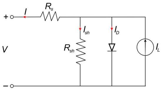
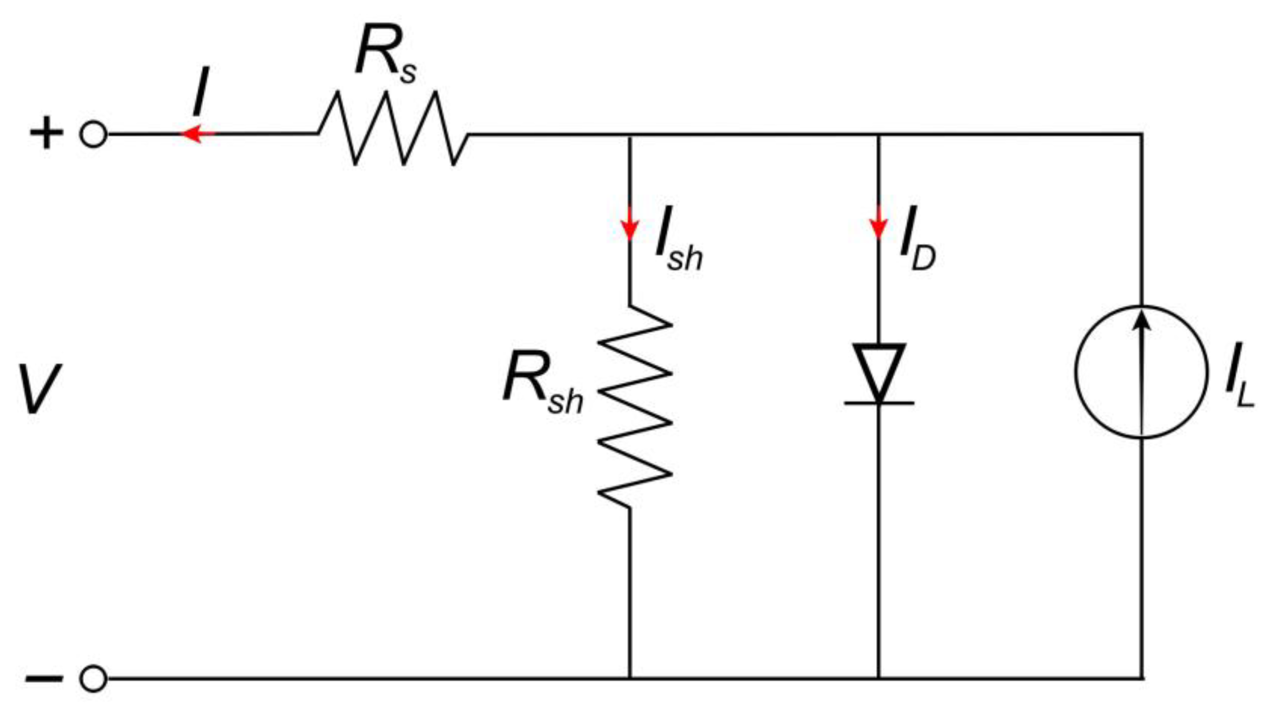
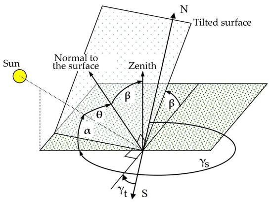
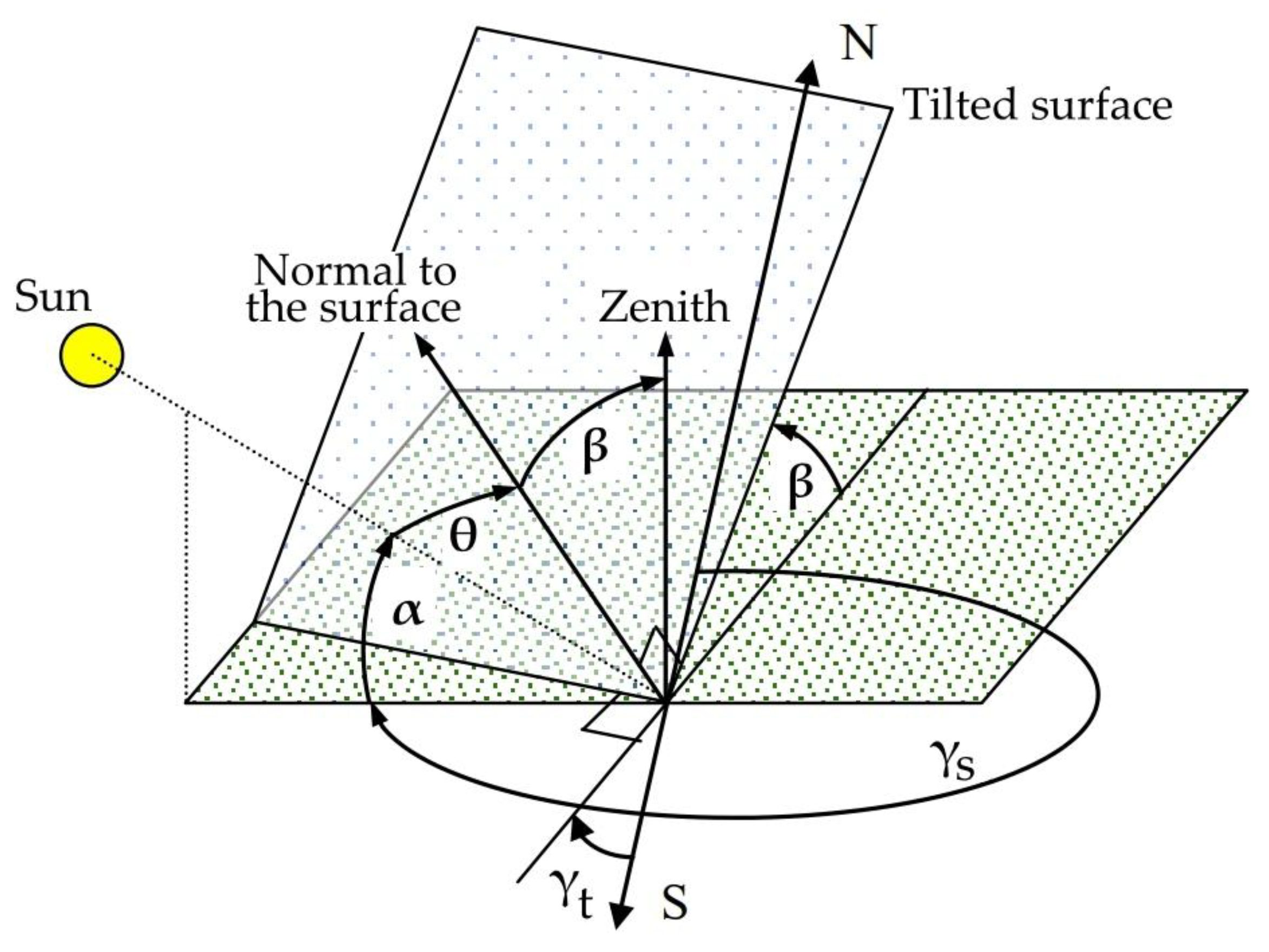
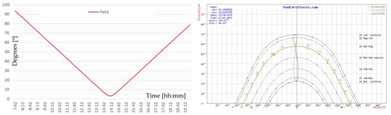
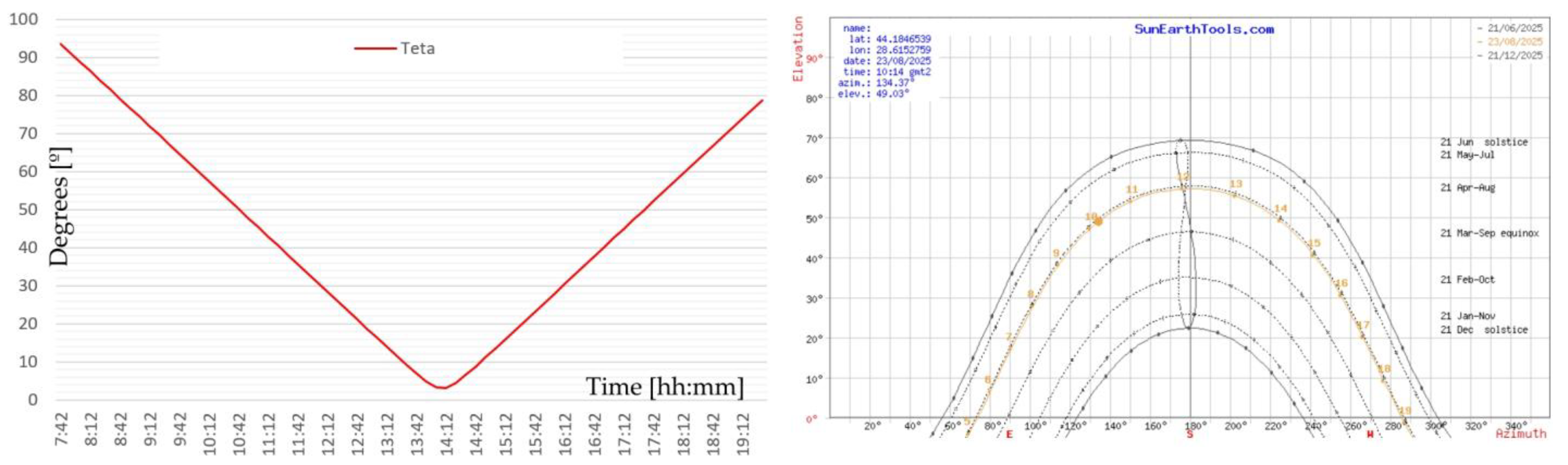
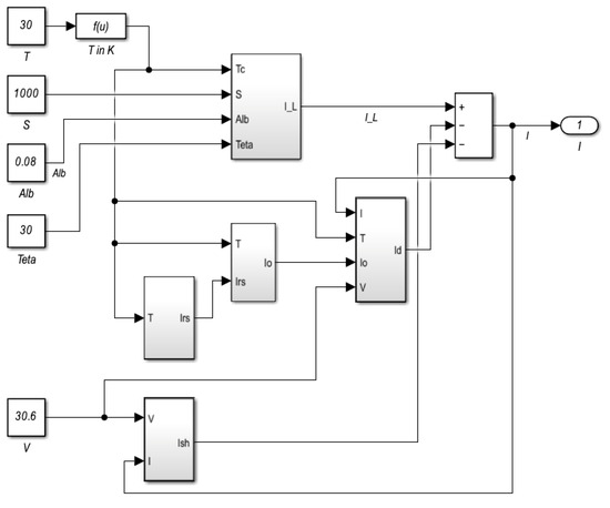
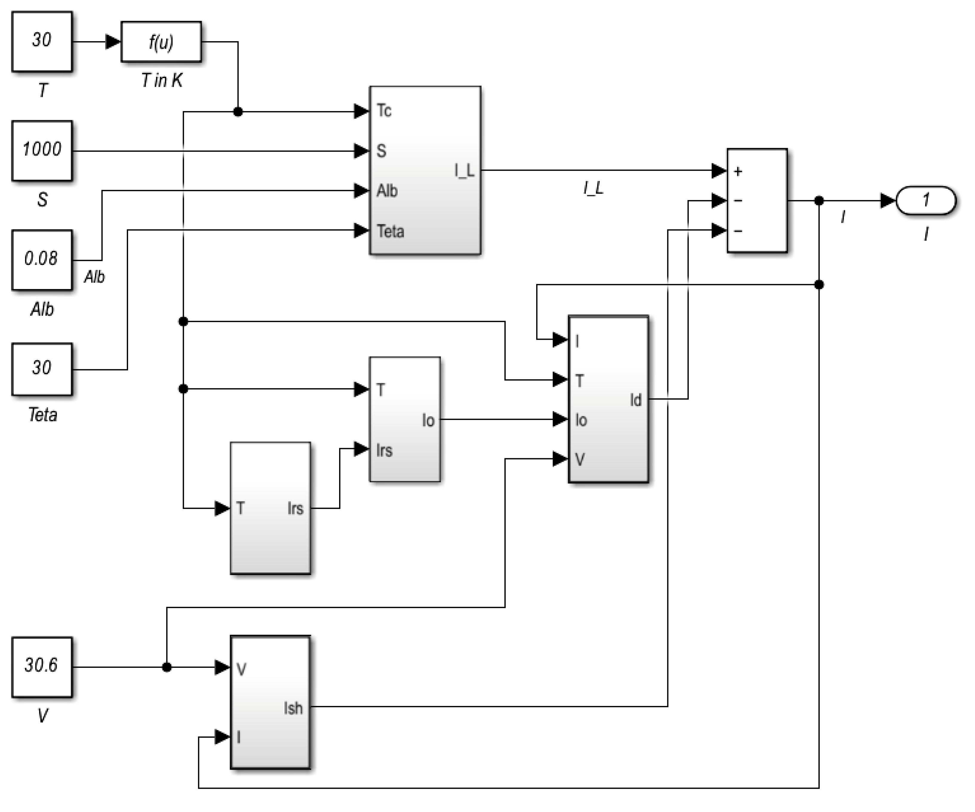
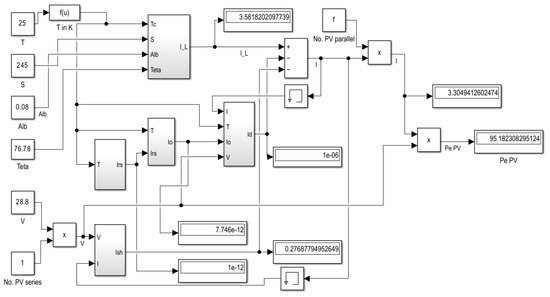
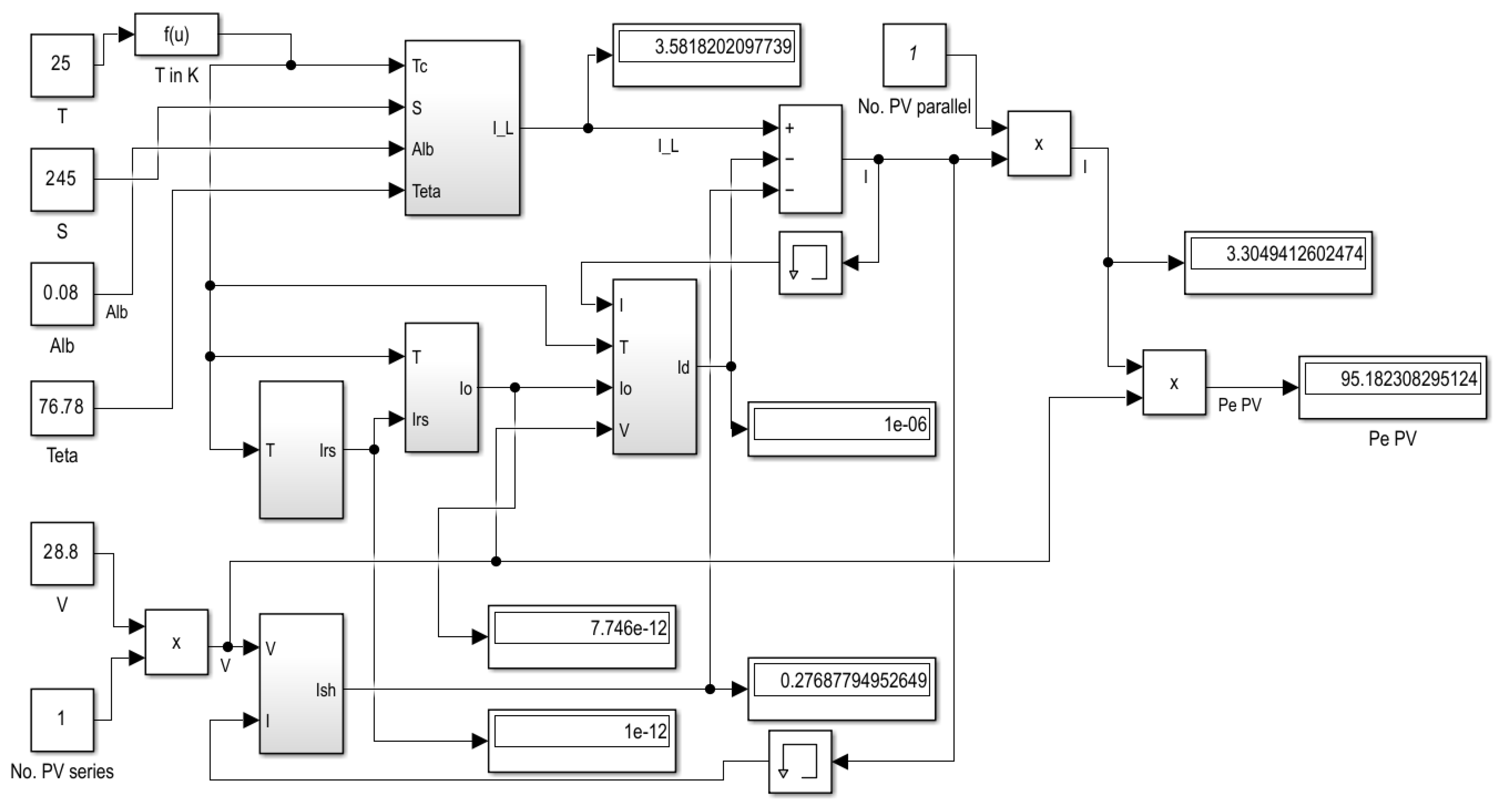
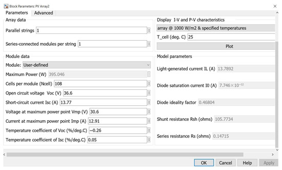
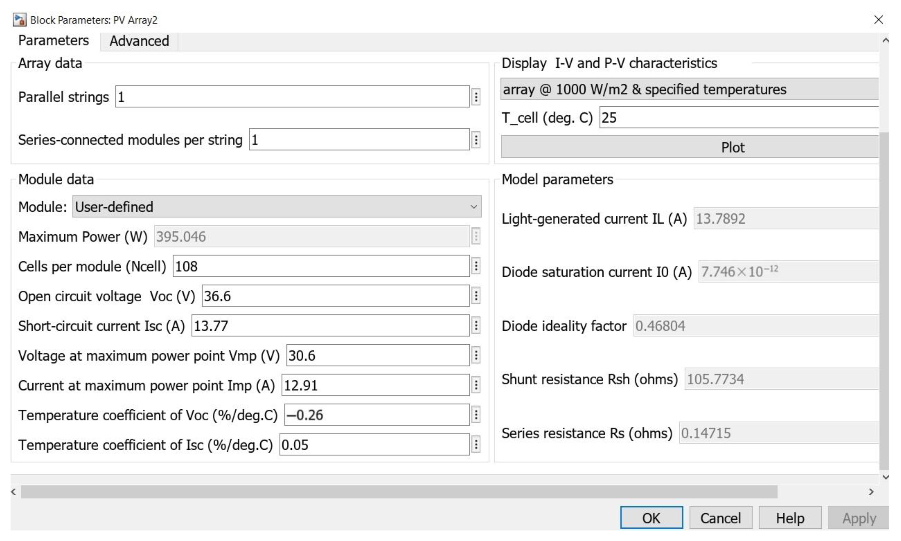
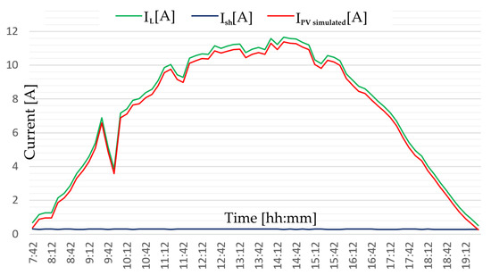
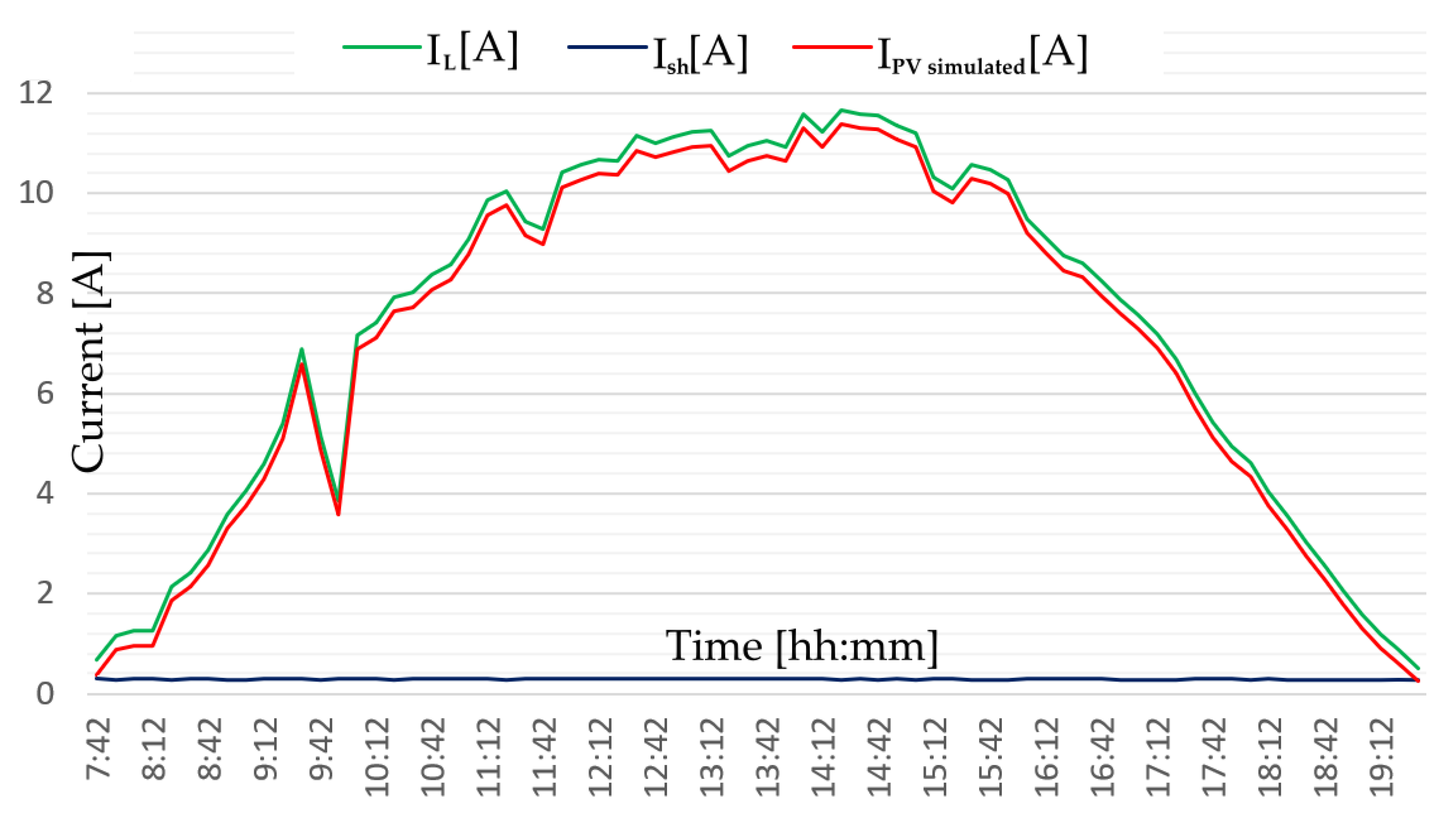
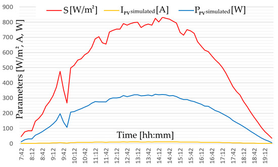
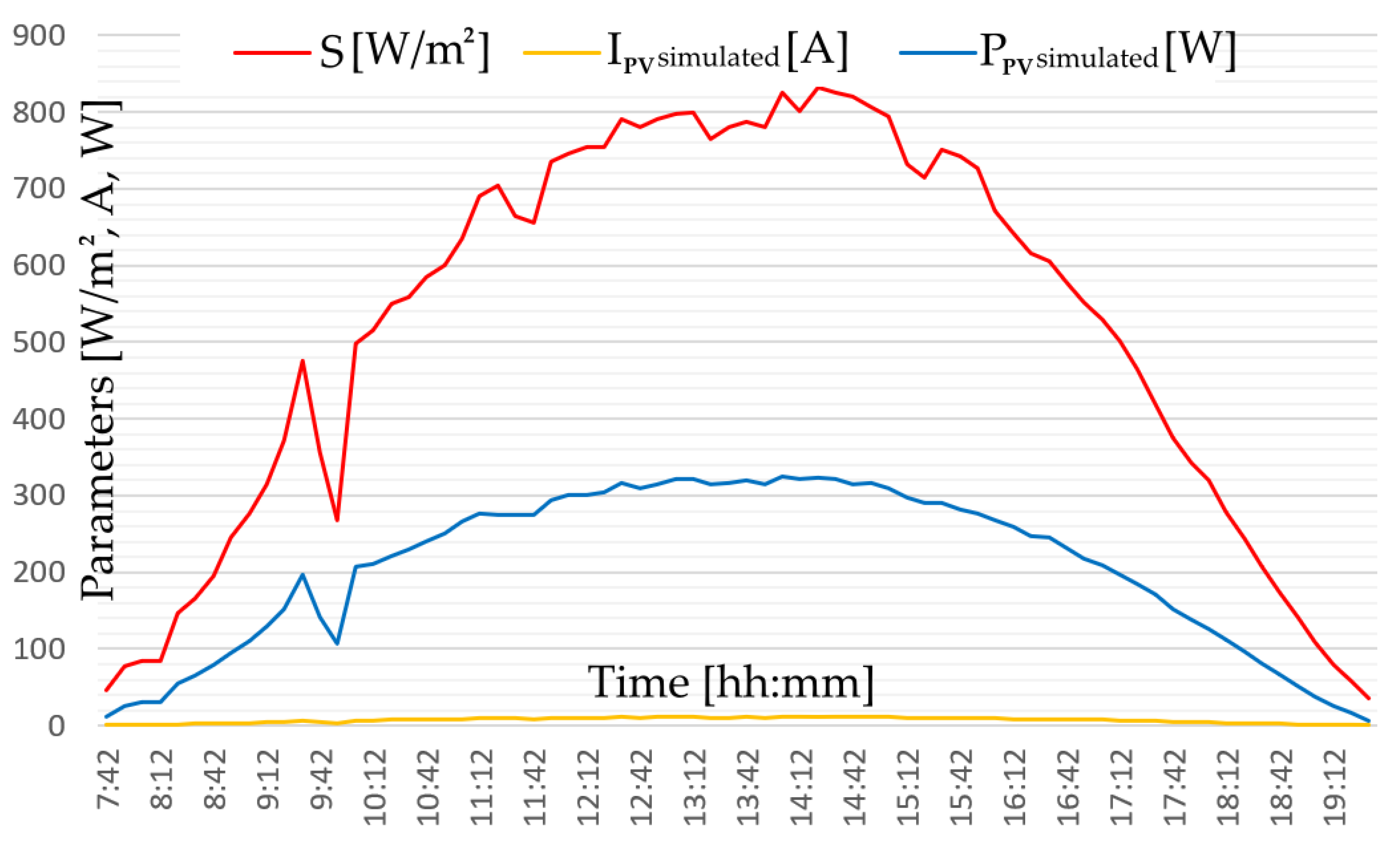
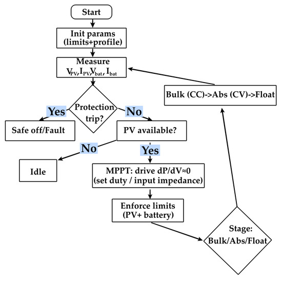
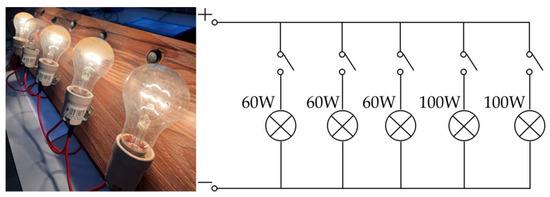
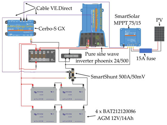
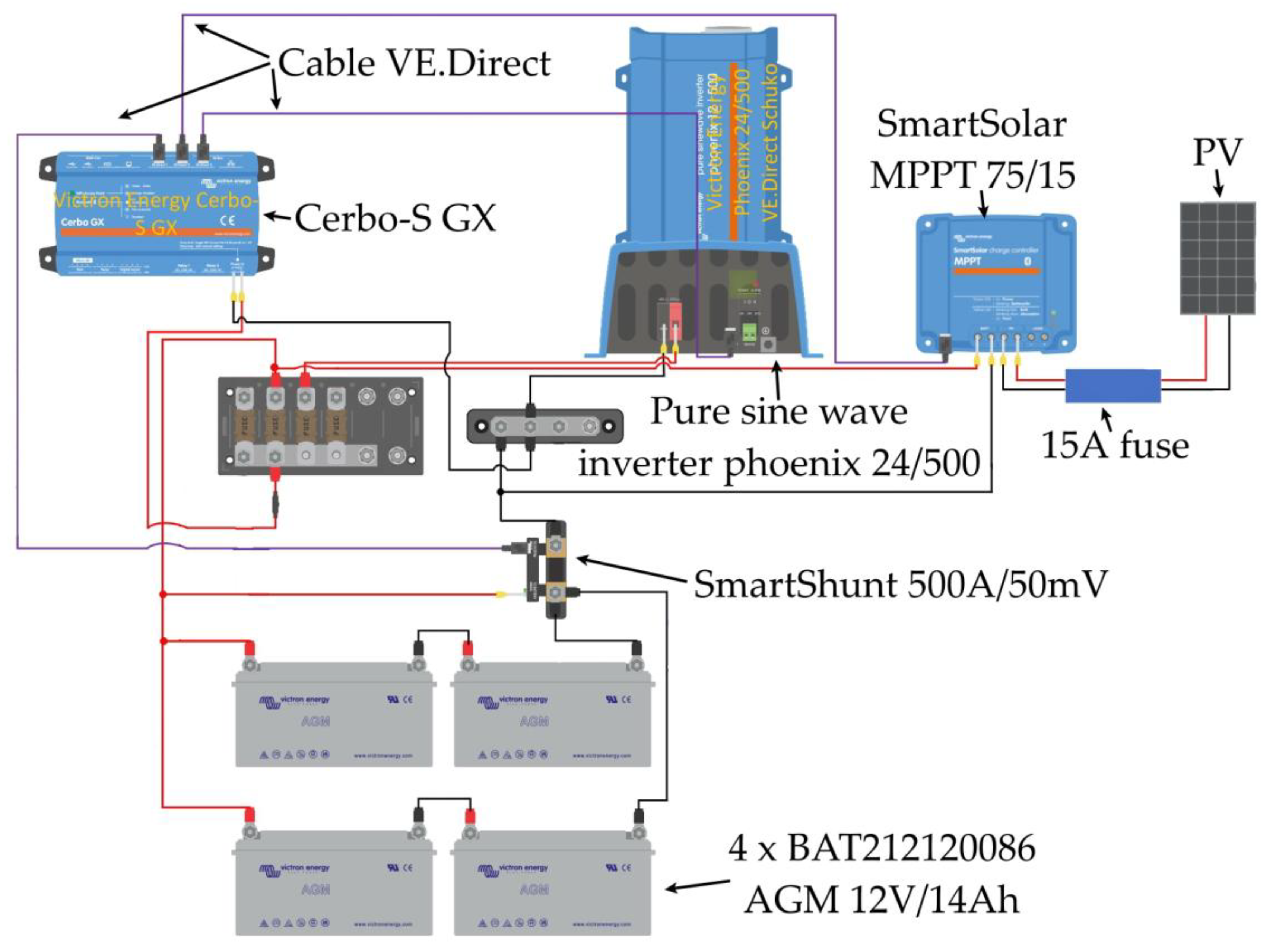
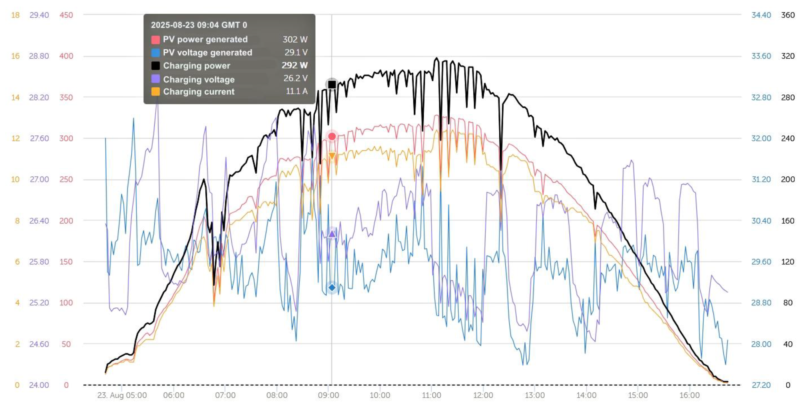
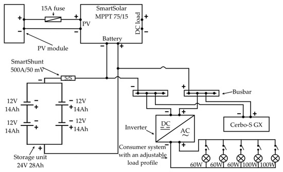
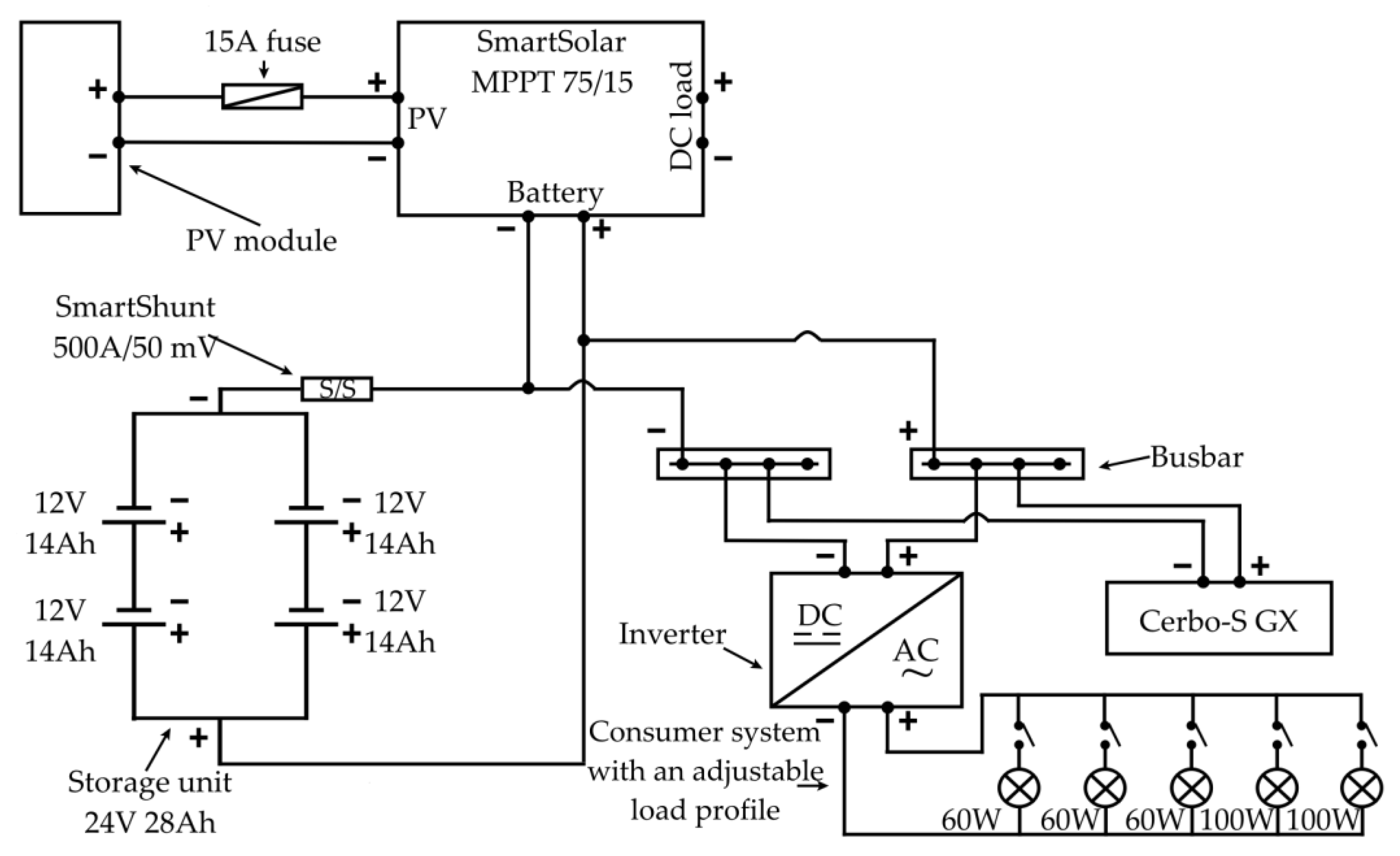
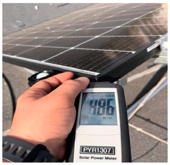
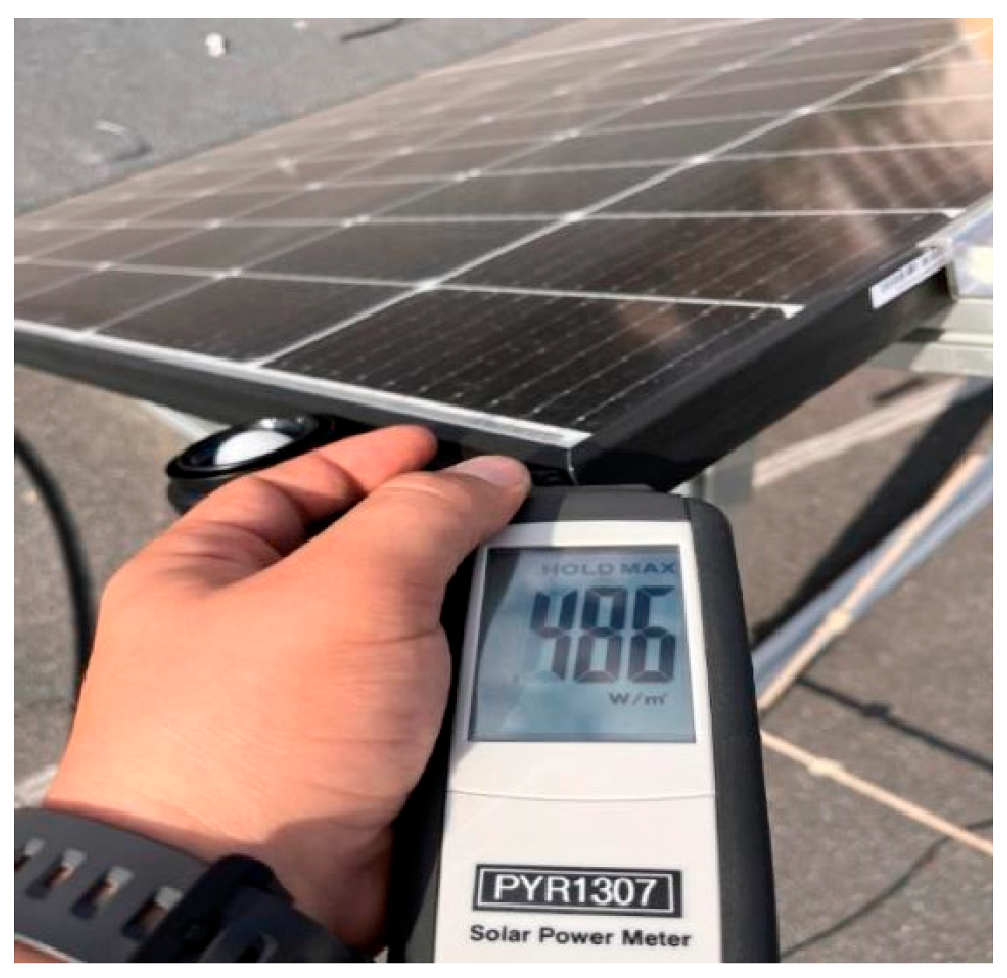
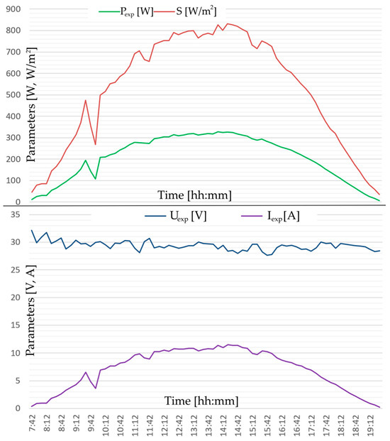
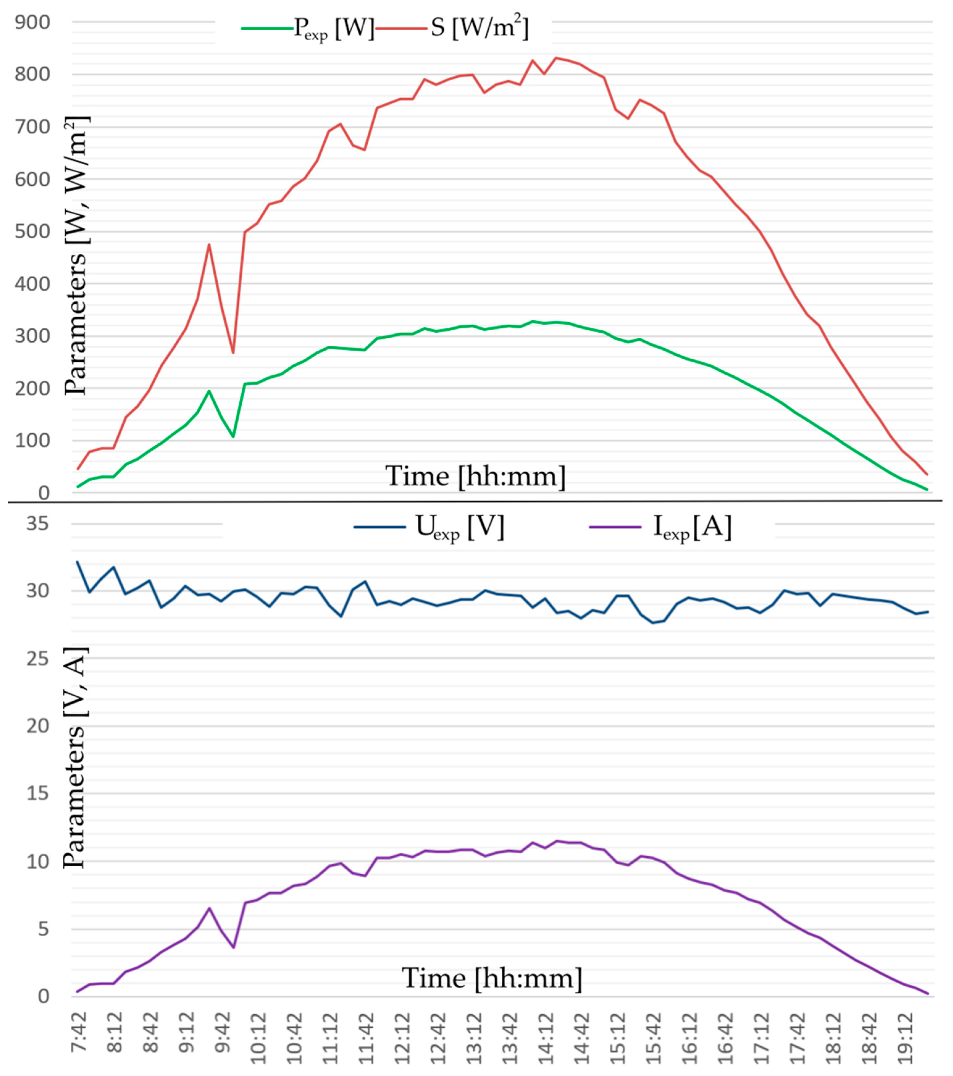
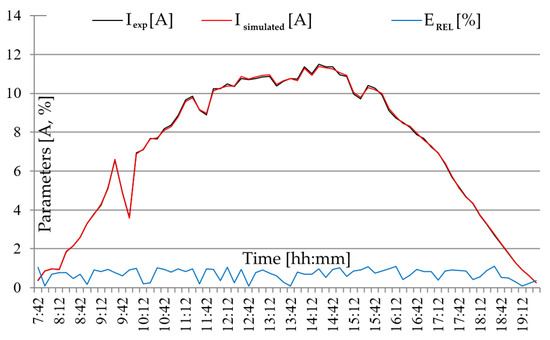
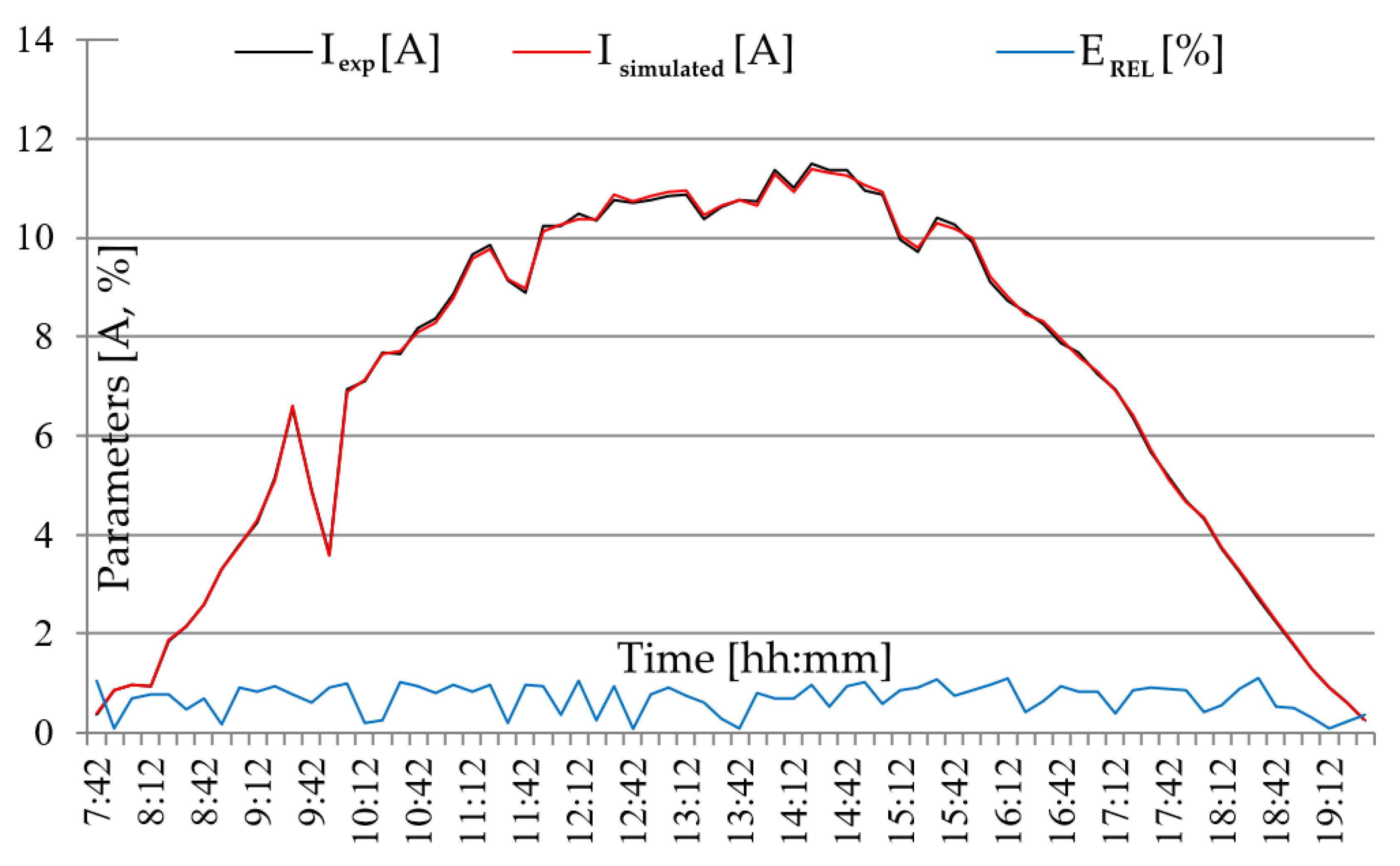
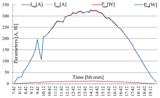
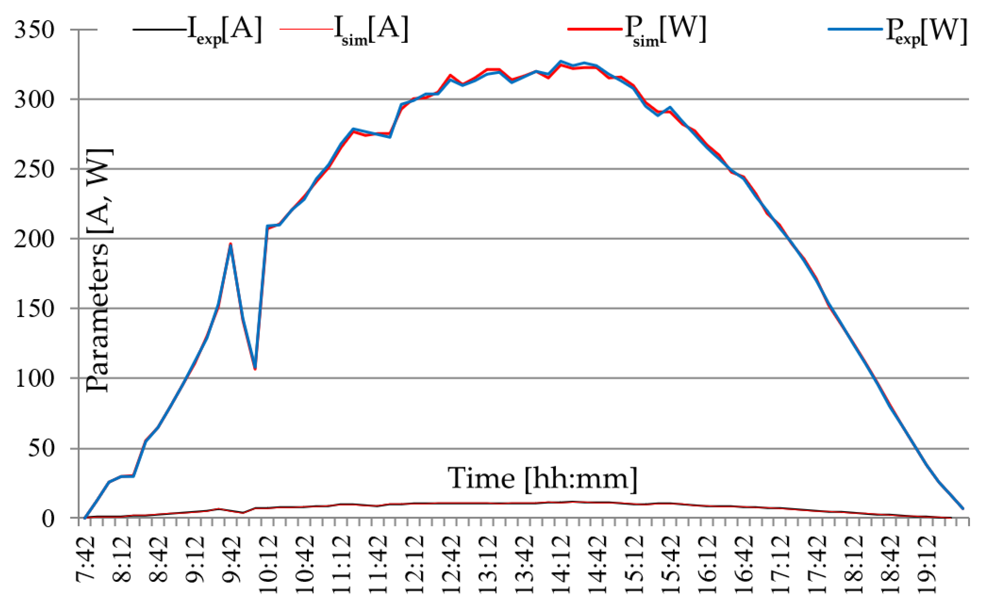

Disclaimer/Publisher’s Note: The statements, opinions and data contained in all publications are solely those of the individual author(s) and contributor(s) and not of MDPI and/or the editor(s). MDPI and/or the editor(s) disclaim responsibility for any injury to people or property resulting from any ideas, methods, instructions or products referred to in the content. |
© 2026 by the authors. Licensee MDPI, Basel, Switzerland. This article is an open access article distributed under the terms and conditions of the Creative Commons Attribution (CC BY) license.