Abstract
Climate change and increasing greenhouse gas emissions are driving the global transition to clean energy, with solar energy experiencing the fastest growth among renewable sources in 2024. Solar PV for energy generation in Kenya is gaining momentum as the country moves towards achieving 100% clean energy by 2030. As solar PV penetration in the grid grows, it is necessary to evaluate its impact on system costs to inform policy decisions on capacity expansion options in the Least-Cost Power Development Plan (LCPDP). This study investigates the effect of large-scale solar PV expansion on electricity costs using the Open-Source Energy Modelling System (OSeMOSYS), a modular, bottom-up capacity expansion model. Four scenarios were developed to assess different levels of solar PV penetration: business-as-usual (BAU), moderate-solar-PV expansion (MSPV), high-solar-PV expansion (HSPV), and very-high-solar-PV expansion (VHSPV). The results indicate that, while overall solar PV expansion significantly contributes to decarbonising Kenya’s electricity mix by displacing fossil-based generation, it also increases annual investment obligations and, consequently, total system costs. The system-levelised cost of electricity (LCOE) is shown to rise by 0.2%, 5.7%, and 14.0% under MSPV, HSPV, and VHSPV, respectively, compared to BAU. Analysing the various cost components against sustainability indicators reveals that the least-cost scenario is BAU while the most favourable scenario based on sustainability indicators is VHSPV, which performs best across technical, environmental, and institutional dimensions but less favourably on economic and social aspects, thereby highlighting a trade-off between sustainability and cost minimisation, at least in the short term.
1. Introduction
Climate change, caused by increasing greenhouse gas emissions, poses a challenge to both humanity and the environment. Global initiatives, such as the 2015 Paris Climate Agreement, have been established to address this issue [1,2] by mitigating the severe impacts of climate change through reducing greenhouse gas emissions. The shift to clean energy is central to achieving these global goals, with many countries actively moving away from fossil fuels towards renewable energy sources such as solar and wind power, which produce little to no emissions [3,4]. Driven by these transitions, renewable energy technologies accounted for the largest share of the increase in total energy supply in 2024, at 38%. Wind and solar accounted for 15% of global electricity in 2024, with solar at 6.9% and wind at 8.1% [5].
Over the past two decades, Kenya’s electricity sector has experienced significant transformation, driven by an ambitious electrification programme and a strong commitment to renewable energy. By 2024, the country’s installed electricity capacity reached approximately 3199.9 MW, with renewable sources, including geothermal, wind, solar, and hydro, making up nearly 90% of the total [6,7,8]. This increase in generation capacity can be linked to a rising electricity demand, with Kenya’s peak demand reaching 2228 MW as of July 2024 [9]. Electricity access in Kenya increased from 32% in 2013 to approximately 84% in 2023 [10], with the intention of achieving universal access by 2030 [11,12]. The government has also adopted a strategic plan to reach 100% clean electricity by 2030, in which utility-scale solar photovoltaic (PV) systems will play an increasingly vital role in Kenya’s efforts to establish a sustainable, resilient power system. As of June 2024, the total grid-interconnected utility-scale solar PV capacity was 210.3 MW, but the Least-Cost Power Development Plan (LCPDP 2024–2043), the current electricity sector development plan, projects an additional 242.5 MW capacity of solar PV from seven power plants by 2030 [13,14].
Kenya has high power potential for solar energy, estimated at almost 15,000 MW [15], supported by insolation levels ranging between 4 and 6 kWh/m2 per day. This is primarily due to its proximity to the equator, with daily sunshine hours averaging 5 to 7 h [15]. By leveraging this solar resource, Kenya is advancing utility-scale solar PV development to diversify its energy mix, reduce dependence on fossil fuels, and strengthen energy security [16].
However, this increased reliance on variable renewables (VREs) presents operational challenges for grid management, requiring infrastructure upgrades to handle variability and to maintain reliability [17,18]. However, though grid reinforcement is critical to prevent bottlenecks in renewable energy integration, expansion efforts must be aligned with national priorities to avoid exacerbating electricity costs [19]. This is particularly important given that Kenya has some of the highest electricity tariffs in the region, with households paying approximately USD 0.222 per kWh as of March 2025 [20] compared to USD 0.171, USD 0.091, and USD 0.201 for Uganda, Tanzania, and Rwanda, respectively [21].
The main objective of this paper is therefore to evaluate the impact of utility-scale solar PV expansion on electricity costs in Kenya, with a focus on both cost and sustainability. It aims to address the following research questions:
- How do generation capacity, energy mix, CO2 emissions, and investment costs in Kenya change under different levels of solar PV penetration, and what are the implications for the total system costs?
- What are the economic, technical, environmental, social, and political implications of increasing utility-scale solar photovoltaic (PV) penetration in Kenya?
1.1. Problem Statement
The increasing penetration of utility-scale solar PV has significant implications for electricity tariffs in Kenya, which are primarily structured around a cost-recovery model where generation costs form a substantial portion of the base tariff [15]. Thus, as solar PV capacity expands, a crucial need arises to thoroughly understand its impact on overall electricity costs, particularly on consumer affordability and the long-term sustainability of the energy sector. Existing energy transition studies primarily focus on broad energy transition pathways [17,22,23,24,25,26,27], overlooking the specific cost implications of utility-scale solar PV expansion.
Given Kenya’s already high electricity tariffs compared to its regional neighbours, a comprehensive understanding of how increasing utility-scale solar PV penetration affects overall system electricity costs is essential for informing effective policy and investment decisions that support both the energy transition and economic development.
1.2. Rationale of the Study
Energy planning in Kenya is primarily guided by the Least-Cost Power Development Plan (LCPDP), a framework designed to ensure the country’s electricity demand is met efficiently and cost-effectively over the long term [28,29]. The LCPDP outlines power system development and capacity expansion projections, typically covering a 20-year horizon, with medium-term plans spanning five years to guide near-term actions [30,31].
By evaluating the cost-effectiveness of solar PV deployment, the study provides essential insights to support investment decisions within the Least-Cost Power Development Plan (LCPDP) framework, helping to identify strategies to minimise overall system costs [32,33].
The findings will also aid key stakeholders, such as the Ministry of Energy and the Energy and Petroleum Regulatory Authority (EPRA), in setting achievable renewable energy targets and updating regulatory frameworks to reflect the current economic and technical realities [31,34].
By modelling potential emissions reductions, the study supports Kenya’s target of achieving 100% renewable electricity by 2030 and enhances its position to attract international climate finance [35,36]. Furthermore, the study contributes to the academic and research community by offering a data-driven case study on energy transition in a sub-Saharan African context, enriching the literature on renewable energy power system modelling and sustainable development planning [33].
1.3. Novelty and Contribution of the Study
Various studies have analysed the expansion of solar PV using various modelling approaches. Using SWITCH-China, a study in 2020 by [37] indicated that rapid declines in PV and storage costs could enable non-fossil sources to supply 62% of electricity by 2030 at a lower cost than business-as-usual, with substantial emission reductions technically achievable by 2030. However, in the same year, a study in Korea [38] employing a stochastic approach demonstrated that current PV generation remains relatively costly, with LCOE estimates of 10–18 US cents per kWh and a high sensitivity to capital costs.
In 2021, another study based in China [39] employed a long-term spatiotemporal model, which demonstrated that ongoing cost reductions and technological advancements could increase technical potential from 99 PWh in 2020 to 146 PWh by 2060, while reducing costs from 4.9 to 0.4 US cents per kWh over the same period. The cost advantage of solar PV enables integration with storage to produce cost-effective and grid-compatible electricity. In the same year, a study in the United States [40] employed a production cost model which demonstrated that coupling PV with battery storage can reduce LCOE and lower emissions by up to one-third.
In 2024, a study in Israel [41] employed an Excel-based energy dispatch model to highlight the operational challenges of achieving a 30% PV share, including increased system inefficiencies, higher backup needs, and slight increases in LCOE, underscoring the importance of flexibility resources at high PV penetration.
In Africa, studies in Morocco and Togo have employed the capacity expansion model, OSeMOSYS, to examine various decarbonisation pathways. The study in Morocco [42] found that a 92% renewable integration is achievable at an additional cost of USD 32 billion, enabled by energy efficiency measures that reduce demand by 15% between 2030 and 2050 relative to baseline projections, while the study in Togo [43] found that photovoltaic and electricity importation are the optimal choices ahead of gas and hydropower.
In Kenya, only a few system-level studies have focused directly on solar PV expansion. Most studies [17,27,44,45] have focused on broad decarbonisation pathways that address renewable energy sources in general, universal access, geospatial constraints, and short-term operational effects. The studies that have been specific to solar PV in Kenya have either been specific to rural electrification [46], mini-grids [47,48], or captive power [49]. The system-level studies specific to solar PV [32,33] employed a simulation model, EnergyPLAN, with the results showing that solar PV could supply 30–40% of Kenya’s electricity, depending on economic and technical limits [19].
These studies, both in the international and regional literature, provide methods for analysing PV potential, integration, economics, and interactions with storage and other renewable alternatives. While some of these methods have been applied in Kenyan studies, solar PV has chiefly been modelled within the context of renewable energy alternatives and a broad capacity expansion pathway for power-sector planning. Solar PV in Kenya is gaining traction due to its modularity, deployment potential, short-term construction timelines, and declining costs. There is therefore a need to understand the impact of utility-scale solar PV on system costs, both in the medium and long term, to plan and anticipate challenges arising from large-scale deployment. Nevertheless, since system costs can only be established within a system, capacity expansion was employed to evaluate how each scenario impacts the overall system. To our knowledge, this is the first study to single out utility-scale solar PV explicitly and to use an expansion model (OSeMOSY) to evaluate two key aspects of the energy trilemma: sustainability and affordability.
Furthermore, beyond cost-optimisation, the study adopts a multi-criteria decision analysis based on the five-dimensional sustainability framework [1], enabling a more comprehensive comparison of expansion pathways. By integrating system-wide optimisation with a multi-dimensional sustainability assessment, the study provides insights into the trade-offs associated with utility-scale solar PV expansion while contributing to ongoing discussions on how solar deployment can enhance affordability, sustainability, and system reliability within the African context.
The rest of the paper is organised as follows: Section 2 introduces energy modelling, outlines the broad classifications of energy models, and discusses the shift towards open-source approaches. It also reviews studies conducted using OSeMOSYS in the region, as well as recent research focused on Kenya that employs energy models. Section 3 presents the materials and methods, including model assumptions, constraints, and the formulated research scenarios. Section 4 presents the model results, which are discussed in Section 5, while Section 6 provides the conclusions and key policy implications.
2. Energy System Modelling
An energy system refers to the complete process of converting primary energy into useful forms for goods and services. Essential elements of such systems include primary energy sources, conversion mechanisms, transmission and distribution networks, storage, and final consumption. These systems can be categorised as centralised, decentralised, or hybrid [50].
Energy system models simplify energy systems to analyse decarbonisation pathways, evaluate technologies, assess policies, study environmental impacts, and support decision-making under uncertainty [50,51,52]. Models vary in type, design, programming, application scope, level of detail, sophistication, and the mathematical optimisation used to guide the solution process. However, they are generally characterised as either bottom-up or top-down, each serving distinct energy and economic purposes [51]. Top-down models examine the present and look back to identify lessons learned and are typically adopted by economists and public administrators. They are used to evaluate the impacts of energy and climate policies on socio-economic sectors such as social growth, public welfare, and employment [51]. Meanwhile, bottom-up models focus on the future and forecast likely changes. These detailed models, from a techno-economic perspective, enable users to compare the impact of different technologies on the energy system and to assess the best future alternatives [51,53].
Bottom-up models serve as analytical tools that simulate and optimise energy systems by emphasising technological and engineering specifics. These models offer detailed insights into energy generation, distribution, and consumption by depicting technologies, costs, efficiencies, and various operational constraints. They find extensive application in policy analysis, energy planning, and scenario evaluation modelling. They are used to represent individual energy technologies and their characteristics and employ mathematical optimisation techniques to find the most cost-effective energy system configuration. They can be customised to capture sector-specific energy demands, such as industry, transport, and residential consumption and are often used to evaluate different policy scenarios, including carbon pricing, renewable energy targets, and electrification strategies [54,55].
The widespread integration of VREs introduces complexities in managing the power system due to its intermittent nature. VREs pose a challenge in maintaining the balance between demand and supply in the absence of storage and backup capacity. This inherent variability directly calls for integrating flexible sources to enhance system resilience. Various modelling tools, with varying levels of detail, are available for designing energy system models for the sustainable integration of RES into the national energy system. They are differentiated based on five main parameters: energy sector covered, geographical coverage, time resolution, methodology applied, and programming technique employed [51].
Models on public policy have been criticised for being opaque or insufficiently transparent to users. As a solution to this challenge, the source code and datasets developed and used should be made available for peer review, and, if possible, published for wider access and acceptance. To achieve greater transparency and thus acceptance, some models can be provided as open-source software projects, often developing a diverse community as they progress, for example, OSeMOSYS [53].
Open-source energy modelling frameworks enhance transparency and credibility by allowing public access to model assumptions, data, and results, thereby enabling independent verification. Their flexible and adaptable design supports modelling across multiple sectors and scales, while collaborative development fosters continuous improvement and innovation. By providing free access to tools and datasets, open-source models reduce duplication of effort, improve quality through shared expertise, and promote broader adoption in the research and policy community [56,57].
Some prominent bottom-up energy models include LEAP, MARKAL/TIMES, MESSAGE, and OSeMOSYS [42], with OSeMOSYS being the only fully open-source energy modelling framework [58]. LEAP is proprietary, but it offers free licences for government and academic institutions in low-income countries [58]. MARKAL/TIMES is not fully open-source since the solver is proprietary [59] while licencing is required to use MESSAGE [60].
OSeMOSYS is a modular, bottom-up modelling and optimisation framework designed primarily for analysing and planning energy systems over the medium and long term. The study by [54] finds that the Open-Source Energy Modelling System (OSeMOSYS) is the leading open-source tool for energy policy analysis, valued for its accessibility, simplicity, and transparency, as well as its modular structure, which allows users to adapt and customise it to their specific needs [59].
In OSeMOSYS, as in other linear programmes, sets, parameters, and variables are defined. The ‘sets’ outline the physical structure of the model, typically independent of the specific scenarios to be executed and fixed across various scenarios. They specify the time domain and time interval, spatial coverage, as well as the technologies and energy vectors to be considered. In contrast, parameters represent the user-defined numerical inputs that constitute the model’s structure. The values of specific parameters are modified when running different scenarios and/or sensitivity analyses [47]. The variables are the model’s output and include demand, storage, capacity, activity, costing, and reserve margins. The complete list and description of all the variables computed by the code of OSeMOSYS are given in [61].
OSeMOSYS has been utilised in numerous energy studies worldwide. For example, Morocco’s electricity system was modelled using OSeMOSYS to evaluate optimal production strategies through 2050, with the model calibrated for the 2015–2017 period to reflect observed production trends [62]. In Colombia, OSeMOSYS was applied to explore technical options and the socio-economic benefits of decarbonisation compared to a business-as-usual (BAU) scenario by 2050 [54]. Similarly, the framework was used to analyse the evolution of the energy mix and the investments required to achieve sustainable energy and climate change goals in Togo by 2050 [43]. The model’s findings revealed that greater energy independence in Togo is attainable, albeit at the expense of increased costs in the electricity system. In Ghana, OSeMOSYS was employed to explore potential pathways for achieving Ghana’s renewable energy production targets amid growing energy demands [63]. The model findings indicated that alternative pathways based on clean energy production may yield cost savings of USD 11–14 billion relative to a business-as-usual case.
A summary of the reviewed studies employing the OSeMOSYS framework and models is presented in Table 1.

Table 1.
Summary of empirical studies employing OSeMOSYS for analysis.
In Kenya, researchers have employed different frameworks and models to evaluate different aspects of the energy sector.
In 2018, OSeMOSYS was employed in a study on socio-economic, geospatially enhanced energy planning, which found that Kenya may not achieve its universal access targets by 2030 [45]. In 2021, a study by [44] developed a new bottom-up energy system optimisation model named Kenya-TIMES. The model was then used to evaluate the implications of the reduction in greenhouse gas emissions on the techno-economic and environmental evolution of Kenya’s power system under different demand levels for the period of 2020–2045. The study findings showed that the higher share of REs under the carbon emission cap scenario results in lower emissions but increased electricity costs. The study recommended that Kenya should develop geothermal and hydropower resources in the short-to-medium term, to provide affordable and secure energy while limiting GHG emissions [44].
A 2021 study developed a LEAP-Kenya-Centralised-Electricity model to assess Kenya’s emission-reduction potential from 2010 to 2040 under six scenarios. The findings show that without major policy shifts, electricity demand and emissions are projected to increase by about 70–80% from 2010 levels, straining the energy system and the environment. Also, while the high-emission pathway requires lower investment costs of around USD 3.1 billion from 2025 to 2040, it results in higher production costs and continued reliance on fossil fuels. In contrast, renewable-based pathways demand higher investments of between USD 12–19.5 billion but achieve up to 90–100% emission reductions, with renewable shares exceeding 98% by 2040 and lower production costs beyond 2030. Although initially more capital-intensive, these renewable pathways provide the most sustainable and cost-effective long-term solution, virtually eliminating PM2.5 pollution after 2035 and supporting Kenya’s transition to a low-carbon electricity system [72].
In 2022, a study was carried out to determine the impact of alternative electricity development pathways on system costs and greenhouse gas emissions in Kenya using the Low Emissions Analysis Platform (LEAP) soft-linked to Next Energy Modelling system for Optimisation (NEMO). The study analysed three scenarios and found that the overall cost savings compared to the LCPDP 2017–2037 were up to USD 26.1 billion dollars, equivalent to 55%, and that, with the high penetration of renewable energy combined with storage, the carbon emission reduction was up to 6.3 Mt [73].
In 2023, a study analysed Kenya’s emission scenarios and pathways toward achieving a net-zero carbon footprint by 2050 using the KCERT 2050 model. The findings were that Kenya will require continuous dedication and collaboration across all sectors of society to realise the full potential of the net-zero scenario. Additionally, due to uncertainties inherent in the model, the author recommended that the model be complemented by other detailed models at the sectoral level, such as the MARKAL and MESSAGE models in the electricity sector [74].
Again in 2023, a study was carried out to determine the significant penetration levels of solar PV on system operations and production costs in Kenya using the EnergyPLAN simulation tool [33]. The study found that large-scale installations of solar PV can decrease CO2-equivalent emissions from 0.134 Mt to 0.021 Mt and that increasing the share of solar PV in electricity generation is possible by as much as 39.56% and 30.54% based on technical and economic considerations, respectively. Additionally, the solar PV electricity produced increased to 19.76 TWh/year from 11.90 TWh/year, with the market economic simulation showing that the total investment annual cost for solar PV could be as low as EUR 10 m/year [33].
In the same year, another study by [24] explored how increasing the spatial and temporal resolution in OSeMOSYS affects energy access. Results showed that a high marginal cost for solar PV with storage during peak periods drives a transition of the system to mini-grid and grid connections when demand levels are high.
In 2024, a study soft-linking OSeMOSYS with Flex-Tool to model power reliability in Kenya confirmed that, based on robust planning approaches, Kenya was well placed to maintain its very-low-carbon generation system under different demand growth projections, leveraging on generation from geothermal and wind sources [17].
Again in 2024, a study by [75] built on the study by [17] to develop an open-source energy modelling system, OSeMOSYS-FlexTool capacity expansion, that explicitly includes the geospatial dimension of VRE buildout and was used to model the Kenyan electricity sector. The model combined capacity expansion planning, geospatial power system planning, and dispatch planning into a single coherent approach. The findings from this study showed that, around 2040, the combination of solar PV and batteries becomes cost-competitive with geothermal and gas power plants. Thus, additional capacity after 2040 will be met by solar, wind, and batteries.
Lastly, in 2025, a study employing the optimisation-based Kenya-TIMES model was used to assess low-carbon strategies for Kenya’s power generation from 2020 to 2050 using a scenario analysis. The study findings indicated that 25 GW of solar capacity is achieved in the tax subsidy scenario, compared to 13 GW in the renewable subsidy scenario and none in the BAU. Also, the scenario with the largest emission cuts was found to be the one with the highest costs and which is thus infeasible without storage. The findings further suggest that combining carbon taxes with subsidies offers the most balanced pathway for low-carbon growth [27].
3. Materials and Methods
The data collected for the study include the historical and forecasted electricity demand data, capacity and operating characteristics of existing generation power plants, energy injected into the grid, cost data for different generation technologies (capital costs, O&M costs, fuel costs), economic parameters to support the discount rates, inflation rates, and electricity prices. Data is sourced through bibliographic research and supported by actual plant performance. The data is then used to build an electricity sector model for Kenya based on the OSeMOSYS framework with defined scenarios to evaluate the impact of solar expansion on electricity costs.
The mathematical formulation of the OSeMOSYS model is based on a partial equilibrium framework that employs linear optimisation. Its primary objective is to minimise the total effective cost of an energy system while meeting a specified energy demand within a given study area, over a defined time horizon, and under predefined constraints [35]. The objective function is derived by summing up all the costs associated with the system [43,63].
The mathematical formulation of the objective function for this study is represented in (1).
where Z = total system cost over the study period, CInvest = investment costs, Com = operation and maintenance costs, Cvar = variable costs (including fuel cost for thermal plants), t = time period (years), and p = generation technology.
The model incorporates capacity constraints by ensuring that each technology has enough capacity to meet its energy production or consumption needs [59]. Electricity generation, use, and emissions are calculated across defined time slices throughout the year to reflect temporal variation.
3.1. Model Constraints and Assumptions
For this study, the modelling user interface for OSeMOSYS (MUIO) ver.5.0.0 was used for analysis. A set of assumptions was established to define the study’s scope:
- The model focused solely on Kenya’s grid-connected electricity sector, excluding other parts of the energy system.
- Electricity demand is aggregated and not broken down by sector.
- A fixed discount rate of 10% is applied throughout the model, based on Kenya’s Central Bank Rate (CBR) [https://www.centralbank.go.ke/].
- Inflation is not considered; all capacity costs are treated as overnight costs.
- The modelling period spans from 2024 to 2040. Although 2024 is in the past, it is included for calibration purposes using available data.
- The straight-line depreciation method, the default in OSeMOSYS, is used.
- All power plants are assumed to operate in a single mode.
3.2. Reference Energy System (RES)
The process of implementing an electricity system model in OSeMOSYS begins with constructing a reference energy system (RES) [59]. The RES is a schematic diagram that illustrates the relationship between fuels, technologies, and demand, providing an overview of the system’s energy flow. It serves as a foundational tool for understanding how OSeMOSYS sets and parameters are connected and what they represent. It does not include numerical data but provides a qualitative framework that captures the core structure and logic of the energy system [76].
In the Kenyan RES, fuel categories are organised into four stages: primary, secondary, tertiary, and final demand. The primary energy sources include both domestic and imported fuels, as well as electricity imports. Generation technologies then convert these primary sources to meet secondary demand, followed by transmission and distribution to end users [77]. In the RES, lines represent energy carriers or services, while blocks represent technologies, as illustrated in Figure 1.
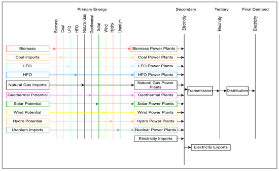
Figure 1.
Kenya electricity sector reference system (Source: adapted from [77]).
The RES in Figure 1 is read from left to right, with the left-hand side showing the primary energy sources. The colours indicate the different technologies in the modelled system, while the arrows show the flow of energy from fuels to final demand. The blocks represent transformation technologies, while the lines represent energy carriers. The lines on the right-hand side represent the electricity demand. For this study, demand is represented as a single gross value rather than being divided into categories to simplify the model. This is because the primary aim of the study is to assess the system-wide impact of utility-scale solar PV on overall electricity generation costs, rather than sector-specific consumption behaviour; thus, an aggregated demand value was deemed sufficient to capture the impact on system costs at the grid level. Furthermore, this model considered only grid-connected generation and excluded distributed energy systems, captive power, and off-grid systems. This specificity to grid-tied utility-scale solar PV could lead to a slight overestimation of grid demand and capacity expansion requirements; thus, the results should be regarded as representative of grid-scale planning effects rather than the overall national energy system optimisation.
3.3. Demand Projections
Demand in OSeMOSYS is determined exogenously and imported into the model for analysis. This study assumed the demand projections as per the reference scenario in the LCPDP 2022–2041 [30]. The LCPDP outlines three demand forecast scenarios for the long-term planning (LTP) period of 2022–2041, using 2021 as the base year. One is the reference scenario, based on historical trends, which anticipates a growth of about 5.28% year on year. The second is the vision scenario, which is based on accelerated growth assumptions aligned with Kenya’s Vision 2030. This scenario assumes the full realisation of flagship projects and an average annual demand of about 8.20%. Lastly, the low-demand scenario assumes minimal economic growth, reflecting a situation where most government plans are not implemented as intended [17,30]. On comparing the different scenarios with historical data, the reference scenario was found to closely align with the actual peak demand from the previous period (2021–2024) and was thus adopted as the demand projection for this study for the period of 2024–2040. This is presented in Table 2.
Table 2.
Total electricity demand in base and final years, with 5-year intervals.
Table 2 shows the demand in 5-year intervals for the modelling period of 2024–2040. It shows demand increasing to a high of 131.17 PJ in 2040, an increase of about 160% from electricity demand in 2024.
3.4. Year Split
The year split parameter defines the duration of each slice within the model. Each time slice represents a unique combination of season, day type, and time band. In Kenya, the climate is typically categorised into four seasons: a dry season, two rainy seasons, and an intermediate season [78]. The duration and corresponding fraction of the year for each season are summarised in Table 3.
Table 3.
Seasons in Kenya.
From Table 3, the longest season is the dry–intermediate period that runs from June to September, with 123 days, and the shortest is the short rain period from October to November, with 61 days.
Furthermore, to capture daily variations in electricity demand, each day is divided into two types: weekdays and weekends. This is because the biggest drivers of electricity consumption in Kenya are the industrial customers [9], and over the weekend, their production is repressed, leading to low-demand periods compared to weekdays. This is again further segmented into three time bands. This classification is based on an analysis of Kenya’s typical electricity demand profile [9] shown and explained in Section 3.6. The time bands adopted for this study are shown in Table 4.
Table 4.
Daily bracket/time bands.
As shown in Table 4, the three time bands chosen for the study are daytime hours, 06:00 h to 18:00 h, when the solar resource is available. The evening peak, when demand is at its highest, occurs between 18:00 and 22:00 h; the off-peak hours, when demand is very low, are between 22:00 h and 06:00 h daily [9].
3.5. Times Slices
For each season, day type, and time band, the model calculates the fraction of the total year represented by that combination, resulting in 24 time slices in total, each defined by a unique combination of the three components. The fraction of the year that each time slice represents is determined by multiplying the respective fractions for the season, day type, and time band. Since there are 4 seasons, 2 day types, and 3 daily time brackets, multiplying them yields 24 time slices. To determine the value of the time slice (fraction), a representative day was randomly chosen for each season and day type, and the actual dispatch data for each time bracket was used to determine the value of the fraction for each of the time slices. Their values are presented in Table 5.
Table 5.
Time slices for the electricity model.
The nomenclature adopted in Table 5 for naming the time slices is such that the first two letters represent the season: S1—dry season, S2—long rains, S3—dry–intermediate, and S4—short rains. The third digit indicates the day type—1 for weekdays and 2 for weekends—while the last digit (1, 2, and 3) represents the daily time band. For example, the time slice S211 represents daytime hours for a weekday during the long rainy season. The use of time slices ensures that energy supply meets demand during each specific period. These time slice values were assumed to remain the same throughout the modelling period.
3.6. Specified Demand Profile
A specified demand profile refers to the annual fraction of energy-service or commodity demand that is required in each time slice. For each year, all the defined SpecifiedDemandProfile input values should sum up to 1. For this study, the demand profile used in the model is derived from Kenya’s actual load data for 2024. A representative day was randomly selected for each of the four seasons and day type, after which, their load profiles were scaled relative to one another to create the final profile. The load profile for a typical weekday in Kenya is represented in Figure 2 [9].
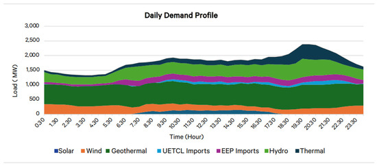
Figure 2.
Representation of a typical load profile for a weekday. Source: [9].
From Figure 2, the daily load curve shows three distinct time periods. The demand starts rising from about 06:00 h, peaks at about 10:00 h, and remains comparatively steady up to about 18:00 h, when the demand starts rising again to form the evening peak at between 08:00 h and 22:00 h, which is then followed by the low-demand period that lasts up to 06:00 h. The resultant demand profile from the above is presented in Table 6.
Table 6.
Demand profile for each time slice.
From Table 6, for each year, all the defined SpecifiedDemandProfile input values must sum up to 1. The demand profile (DMD) shows the annual fraction of electricity demand that is required in each time slice, which allows the model to capture the temporal variability and shape of energy demand throughout the year, thus aligning energy planning with reality. Visualisation of the variation in the demand profile for each time slice is further illustrated in Figure 3.
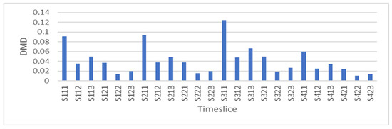
Figure 3.
Specific demand profile.
Figure 3 shows the demand profile across the time slices. This profile is assumed to remain constant throughout the modelling period. The highest demand occurs during the daytime hours of a weekday in the dry–intermediate season (S311) time slice, while the lowest is observed during the peak hours of a weekend in the short rainy season (S422) time slice. The dry–intermediate season is also the season with the lowest temperatures in Kenya [79]; thus, heating needs could be the drivers for the high demand during this season. Furthermore, in Kenya, commercial and industrial consumers are the major drivers of national electricity use, and their operations are typically high on weekdays and significantly reduced on weekends and holidays, hence the variance between energy demand during the weekdays and weekends [9].
3.7. Techno-Economic Parameters
The techno-economic parameters for the different technologies are adopted from the LCPDP 2022–2041 report [30], which is the main planning document for the energy sector in Kenya, and are averaged per technology for 2024. Except for solar and wind technologies, whose costs are revised each year due to their decreasing capital costs, the costs for the other technologies are kept uniform for the entire modelling period. The annual learning curves for solar and wind, according to IRENA [80], are assumed to be 3% and 0.3%, respectively, and are applied to the costs from the beginning of the modelling period to the end. The assumed costs are shown in Table 7.
Table 7.
Techno-economic assumptions for the various power plants.
From Table 7, the capital costs refer to the annualised upfront costs incurred in building and commissioning the power plants to the point of operation and maintenance. The annualised major investment costs of the different technologies are presented in millions of US dollars per GW, while fixed costs are the annualised fixed expenses to keep the power plants running, presented in millions of US dollars per GW. Variable costs are costs associated with production levels and are given in millions of US dollars per petajoules. Wind and solar have reached grid parity and are comparable. Solar PV has high investment and fixed costs, but the variable costs are negligible. The values indicated in this table for solar * and wind * are only values at the beginning of the modelling period before the application of the annual learning curves of 3% and 0.3%, respectively. The capital cost for a liquefied petroleum power plant is zero, since the only existing power plant is already amortised and incurs only fixed operating and maintenance costs and variable fuel costs. With regard to the operational years and the assumed lifecycle of the power plant, the nuclear power plants have the longest lifespan. In OSeMOSYS, the InputActivityRatio defines how much of a specific fuel/commodity is needed to produce one unit of technology activity, and since the output activity ratio is typically set to zero, the efficiency of a commodity/fuel is the inverse of the InputActivityRatio [61]. The average capacity factors for existing technologies were determined using actual dispatch data for 2024 from the National Control Centre in Kenya. The plants indicated with an asterisk either are non-existent in the Kenyan grid or did not run in 2024. The capacity factors were thus adopted from previous studies [17,27].
3.8. CO2 Emissions
In OSeMOSYS, emissions are accounted for using the EmissionActivityRatio (kton/PJ) parameter, which is the mission factor of a technology per unit of activity. For this study, only CO2 emissions were considered, as these are the most common greenhouse gas emissions and were assigned based on the fuels used by each technology. The assumed CO2 emission factors for each technology were borrowed from the planning document for the Kenyan electricity sector, the LCPDP 2022–2041 [30], for uniformity. The emission activity ratio was thereafter determined by dividing the emission factor by the fuel efficiency and is presented in Table 8.
Table 8.
Emission factors for various fuels.
Table 8 shows how different sources of energy have different carbon values, with coal having the highest level of emissions, followed by heavy fuel oil and then gas oil. Natural gas has the lowest level of emissions among the listed fuels.
3.9. Scenarios
For this study, four scenarios with varying levels of solar expansion were developed and used to evaluate the impact of solar expansion on the cost of electricity in Kenya using the OSeMOSYS modelling framework. The scenarios are as follows:
- Business-As-Usual (BAU) Scenario: This is the current situation of the Kenyan electricity sector with the status quo and the planned increases in production up to 2027, to allow for the incorporation of committed power projects, after which the model is left unconstrained to choose the most optimal pathway.
- Moderate-Solar-PV Expansion (MSPV) Scenario: This scenario is based on the BAU scenario, but with solar PV expansion restricted to constitute more than 10% of the capacity mix. The aim is to determine the impact of moderate utility-scale solar PV expansion on electricity costs.
- Scenario 3—High-Solar-PV Expansion (HSPV) Scenario: This scenario is also based on the BAU scenario. Solar PV expansion in the capacity mix is constrained to above 20%. The aim is to determine the impact of high-solar-PV expansion on electricity costs.
- Scenario 4—Very-High-Solar-PV Expansion (VHSPV) Scenario: This hypothetical scenario aims to evaluate the impact on costs when solar PV expansion is above 40% of the capacity mix from 2025 to 2040.
3.10. Model Calibration and Validation
OSeMOSYS is designed to choose the cheapest power generation options unless specific limits are set. However, this study focuses on modelling scenarios based on Kenya’s energy policies and future plans. To reflect this, limits on capacity and generation were adjusted to match the current and expected electricity mix. As mentioned earlier, the Least-Cost Power Development Plan (LCPDP) 2022–2041 is a reference for future projections. Therefore, the business-as-usual (BAU) scenario was calibrated using data from the distribution utility, Kenya Power 2024 Annual Reports for the beginning of the model period (2024), with LCPDP projections used for the period up to 2027.
4. Results
4.1. Reference Scenario Validation
To validate the tool, model output was compared with generation data obtained from Kenya Power, the distribution utility in Kenya, for 2024. The variation between the measured data and modelled results is about 2.12%, which is within range. The model, however, overestimates thermal generation using HFO while underestimating generation from wind and solar PV, as shown in Table 9.
Table 9.
Comparison of modelled and actual data from Kenya Power [9,81].
From Table 9, it is evident that the model slightly underestimates generation from geothermal technologies (0.61 PJ) and significantly overestimates output from thermal HFO (−2.05 PJ). It also marginally overestimates generation from hydro technologies (each within 0.06 PJ) and solar PV (−0.21 PJ), while underestimating wind by 2.48 PJ. These discrepancies likely arise from deriving capacity factors from annual-average dispatch data, which tends to smooth temporal variability in resource availability and operational constraints. As a result, the model may not fully capture short-term variability patterns for variable renewables and peaking thermal plants. However, the deviations are small relative to total system generation and fall within an acceptable range for long-term capacity expansion modelling.
4.2. The Capacity Mix
The Capacity mix in the different scenarios was determined from the TotalCapacityByTechnology variable in the OSeMOSYS model results. By 2040, the BAU scenario forecasts about 8.3 GW of installed capacity, a 164.5% increase from the start of the modelling period. MSPV reaches 8.36 GW, a 0.14% increase over BAU. HSPV hits 8.86 GW, which is about 6.1% above BAU, while VHSPV is 19.7% higher at about 10.0 GW. This trend is represented in Figure 4.
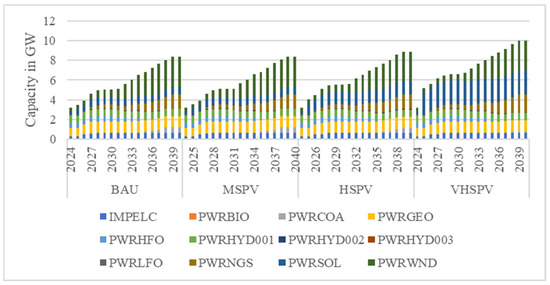
Figure 4.
Installed capacity per technology in the BAU, MSPV, HSPV, and VHSPV scenarios (source: model results).
Figure 4 indicates that, in 2040, wind, natural gas, and geothermal are the dominant technologies in the BAU and HSPV scenarios. However, in the HSPV and VHSPV scenarios, solar PV displaces geothermal to become the third- and second-most dominant technologies, respectively. Natural gas is introduced into the mix in 2027 across all scenarios, while coal is delayed to 2034, 2036, and 2037 in the MSPV, HSPV, and VHSPV scenarios, respectively. This points to higher-solar-PV penetration leading to greater emission reductions, since the deployment of coal, which has a high emission intensity, is delayed in the higher-solar-PV scenario compared to BAU. Coal accounts for 10.4% of all additional capacity during the modelling period in the BAU but only 1.9% in the VHSPV scenario.
4.3. Generation Mix
The evolution of the generation mix across the different scenarios is evaluated using the ProductionByTechnologyByMode variable in the OSeMOSYS results. Solar PV accounts for about 6.1%, 6.27%, 10.88%, and 20.09% of generation in the BAU, MSPV, HSPV, and VHSPV scenarios, respectively. The dominant technologies across all scenarios are wind, imports, and geothermal, except in the VHSPV scenario, where solar PV generation outperforms both geothermal and imports, ranking second in the generation mix after wind. This is represented in Figure 5.
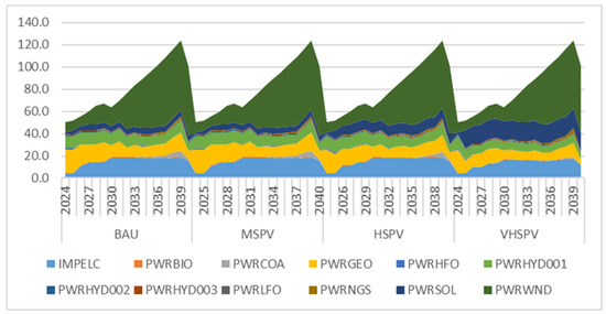
Figure 5.
Generation mix in the BAU, MSPV, HSPV, and VHSPV scenarios (source: model results).
In Figure 5, demand across all scenarios is held constant and rises steadily to its peak in 2039. In the VHSPV scenario, the average contribution of solar PV to the generation mix in the model period is about 20.09%, which is about 14% more than in the BAU scenario. With the increase in solar PV generation, a reduction in the generation share of almost all other technologies is observed, except for natural gas, which indicates an increase of about 0.22% compared to BAU. The notable reductions are from geothermal, wind, and major hydro technologies, at 4.33%, 3.33%, and 3.04%, respectively, compared to BAU. As total demand is unchanged across the scenarios, the additional generation from solar PV must substitute output from other technologies for the system to remain in balance. The model therefore shifts generation away from coal with higher system costs and lower operational flexibility to natural gas during periods of high solar output. The marginal increase in generation from natural gas is due to its low system cost and flexibility to balance solar variability.
4.4. Emissions
The AnnualTechnologyEmission variable in the OSeMOSYS results is used to compare emissions across the scenarios. The cumulative carbon dioxide (CO2) emission for the modelling period is approximately 5684.14 ktons in the BAU scenario. This decreases progressively across the scenarios to 5645.84 kTons, 4655.08 kTons, and 2939.56 kTons in the MSPV, HSPV, and VHSPV scenarios, respectively. This trend is shown in Figure 6.
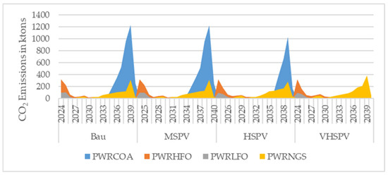
Figure 6.
Total emissions in the BAU, MSPV, HSPV, and VHSPV scenarios (source: model results).
Figure 6 shows that, in the model period, the percentage reduction in overall emissions compared to the BAU scenario is 0.7%, 18.1%, and 48.3% for MSPV, HSPV, and VHSPV, respectively. In terms of specific fuels, emissions from coal technologies are dominant in the low-solar-PV scenario, contributing about 3538 kton of CO2 emissions in the BAU scenario compared to about 500 kton in the VHSPV scenario, a difference of about 86%. In the model period, the share of CO2 emissions from coal is 62.2%, 61.4%, 51.4%, and 17% in the BAU, MSPV, HSPV, and VHSPV scenarios, respectively. On the other hand, the share of emissions attributed to natural gas increases in higher-solar-PV scenarios. In the VHSPV scenario, natural gas accounts for 46.5% of total emissions, compared to 25.6% in HSPV and 18.3% in BAU. Since demand across the scenarios is the same, as coal generation is reduced more aggressively, natural gas assumes a greater role in providing flexibility and balancing services to accommodate solar PV variability, due to its comparatively lower system costs, indicating a relative shift in the remaining fossil-based generation mix. Substituting coal with natural gas in high-solar scenarios reduces overall emissions, as natural gas has a substantially lower emission factor than coal. Therefore, even when gas generation increases marginally to support system flexibility, the net effect is a significant reduction in overall emissions as solar PV penetration rises.
4.5. Investment Costs
The AnnualizedInvestmentCost in the OSeMOSYS results is the variable used to determine the investment cost requirements over the modelling period. Investment costs in the modelling period increase progressively each year and also across the four scenarios. In the BAU scenario, the cumulative investment is 6820.73 MUSD, while in the MSPV, HSP and VHSPV scenarios, it is 6838.76 MUSD, 7470.86 MUSD, and 9042.36 MUSD, respectively. The annualised investment costs in five-year periods for each scenario are shown in Table 10.
Table 10.
Annualised investment costs for the BAU, MSPV, HSPV, and VHSPV scenarios in MUSD.
Table 10 only includes costs for new investments in the modelling period; it does not include residual investment costs at the beginning of the modelling period. Thus, the differences across scenarios reflect the incremental capacity additions required to meet growing demand and scenario-specific constraints and not total system costs. Compared to BAU, the investment costs for the MSPV, HSPV, and VHSPV scenarios for the modelling period are higher by 0.3%, 9.2%, and 21.0%, respectively. The spread of the investment costs across technologies in different scenarios is shown in Figure 7.
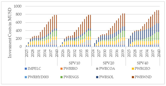
Figure 7.
Investment cost for the period of 2024–2040 for the BAU, MSPV, HSPV, and VHSPV scenarios (source: model output).
From Figure 7, in the BAU and MSPV scenarios, wind accounts for over 38% of new investment costs, making it the largest contributor, followed by geothermal at around 18%, and natural gas at approximately 12%. Investment costs for solar PV in these two scenarios are about 11%. In this scenario, geothermal remains the primary baseload option, but as solar PV adoption increases in the HSPV scenario, the makeup of investment costs changes. Wind remains a substantial cost factor, but its share decreases to around 32%, while solar PV investment increases to about 22%. Geothermal and natural gas retain relatively steady shares of approximately 17% and 13%, respectively, indicating ongoing investment in reliable, flexible capacity to support the growing share of variable solar generation.
However, in the VHSPV scenario, solar PV becomes the primary driver of investment costs, representing more than 37% of total new investments. This highlights the extensive deployment of utility-scale solar PV necessary to attain very high penetration levels. Wind remains the second-largest contributor at around 26.1%, while investments in geothermal and natural gas decrease to 14% and 13%, respectively. This shift demonstrates a move towards a solar-led investment pathway, supported by investments in wind, geothermal, and flexible gas generation to ensure system reliability.
Overall, the results show that higher-solar-PV ambitions lead to increased investment requirements and a reallocation of capital towards solar technologies, which, during the modelling period, has been shown to increase total investment costs.
4.6. Scenario Comparison Using Multi-Criterion Decision Analysis
To compare the different scenarios based on sustainability pillars, the following key performance indicators were used:
- (a)
- For the economic pillar, the total additional investment costs for the model period, which are the upfront costs which need to be considered to deploy the various solar PV levels for investment planning, serve as the indicator to compare the scenarios.
- (b)
- For the social pillar, the system LCOE, which indicates the average cost of generation and indirectly reflects the affordability of electricity, is employed. It is calculated as shown in (2) below (the formula assumes the costs derived from the model to be already discounted).
- (c)
- For the technical pillar, the average reserve margin (RM) for the model period for each of the scenarios is used as the key performance indicator. RM is a measure of the system’s ability to meet demand and system shocks arising from increased VREs [82]. It is computed using (3) below.
- (d)
- For the environmental pillar, total CO2 emissions for the model period, which are a direct output from the OSeMOSYS model, are used as the key performance indicator.
- (e)
- Lastly, the percentage reduction in fossil fuels in the energy mix is used as an indicator for the institutional/political pillar since it is an indicator of the progress made towards 100% green energy generation by 2030 and the net-zero global goals. This is determined by the difference between the share of fossil fuel generation at the end of the modelling period (2040) compared to the share of fossil fuel generation at the beginning of the model period (2024) for each of the scenarios.
The results of the above indicators are presented in Table 11.
Table 11.
System-level KPI results.
The weighted sum model (WSM) approach in multi-criteria decision analysis is then used to summarise the key performance indicators across the different scenarios and determine the optimal one. For ease of interpretation, the performance indicators were assumed to carry equal weight. The results are summarised in Table 12.
Table 12.
Comparison of solar PV expansion scenarios based on the sustainability pillars.
Table 12 shows that the scenario with the highest score is VHSPV at 0.917, while the scenario with the lowest score is BAU at 0.844. VHSPV scores highly on climate goals, the percentage reduction in the use of fossil fuels, and the reduction in overall CO2 emissions. The reserve margin is also highest in the VHSPV scenario. While BAU has the lowest MCDM score, it scores highly in absolute cost terms, such as the system LCOE and investment costs. Based on the above, BAU is the least-cost scenario while VHSPV is the most optimal, taking into account the five-dimensional sustainability criteria.
4.7. Sensitivity Analyses
Sensitivity analyses were conducted based on the discount rate and capital costs for solar, coal, and natural gas to determine which parameter is most influential regarding changes in the LCOE and emissions. The BAU and VHSPV scenarios were used as representative marginal scenarios to evaluate the sensitivity. Results from varying parameters were compared with their respective scenario outcomes.
4.7.1. Effect of Discount Rate
All the scenarios were run with the assumption of a flat 10% discount rate. To assess sensitivity, the discount rates were set to 8.5% and 12.5% to analyse the outcomes. The 12.5% is the assumed return on investment for public-sector power plants in Kenya. It can be seen in Table 13.
Table 13.
Sensitivity analysis on discount rates for energy projects.
Table 13 shows that, while a lower discount rate (8.5%) has a marginal effect on LCOE in both the BAU and VHSPV scenarios, ranging from 0.1% to −1.8%, it significantly impacts emissions, reducing them by between 10.4% and 6.5%. Conversely, at a higher discount rate (12.5%), the change in LCOE is about 14% in the BAU scenario and 15% in the VHSPV scenario. The reduction in emissions at this rate is marginal, between 0.6% and 1.1%. A low discount rate encourages greater deployment of renewable energy technologies because their low operating costs outweigh their relatively high upfront capital requirements. As a result, under the BAU scenario, a lower discount rate leads to increased renewable energy penetration and corresponding reductions in GHG emissions. In contrast, a higher discount rate favours technologies with lower capital costs but higher operating expenses, thereby limiting renewable energy uptake.
4.7.2. Effect of Solar PV CAPEX
The solar CAPEX assumed for this study was based on actual costs in the LCPDP 2022–2041, with the rate at the start of the model period being the average for the technology at 1128 USD/kW, reducing at a constant rate of 3% annually throughout the modelling period. To assess the sensitivity of solar CAPEX costs on LCOE and emissions, a higher CAPEX based on a study by [33] was adopted. The study assumed a CAPEX of 1150 USD/kW; the same 3% reduction factor was applied annually to address reducing CAPEX for solar PV. For the lower-solar-PV CAPEX, this study adopted the projections by IRENA [83] for the period of 2024–2029, after which the 3% reduction factor is applied up to the end of the modelling period. The CAPEX at the start of the modelling period for the lower-CAPEX scenario is 691 USD/kW. The results are shown in Table 14.
Table 14.
Sensitivity analysis for solar PV CAPEX.
Table 14 shows that, in the BAU scenario, a reduction in solar PV CAPEX affects both LCOE and emissions. Although LCOE increases by 3.8% relative to the base modelling results, emissions decline substantially by 52.4%, indicating that lower upfront investment costs enable higher deployment of cleaner generation technologies that displace higher-emitting options. In the VHSPV scenario, a lower CAPEX reduces LCOE but has no significant impact on emissions, since solar PV already dominates the system. In contrast, a higher solar CAPEX increases LCOE in both the BAU and VHSPV scenarios, while emissions remain largely unchanged. This shows that changes in solar PV costs affect system costs but only affect emissions in low-solar-penetration scenarios; no significant impact is found in high-renewable-energy systems.
4.7.3. Effect of Increase in Coal and Natural Gas Prices
A study by [17] adopted a higher cost for both coal and natural gas technologies at 2500 USD/kW and 1350 USD/kW compared to the 2079 USD/kW and 1133 USD/kW adopted for the base model. These numbers were used to test the sensitivity of the model results to higher costs of natural gas and coal prices, and the results are presented Table 15.
Table 15.
Sensitivity analysis for coal and NGS costs.
Table 15 shows that a 20% and 19% increase in coal and natural gas costs results in a 7% and 6.8% rise in LCOE in the BAU and VHSPV scenarios, respectively. In contrast, emissions decreased by 38.8% and 16.2% in these scenarios. This indicates that higher fossil fuel costs, such as the introduction of carbon taxes, favour the deployment of renewable energy technologies, as seen in the greater reductions in emissions under high-solar-PV scenarios. This finding, however, highlights a trade-off between environmental and climate goals and socio-economic factors such as electricity costs.
5. Major Findings and Discussion
5.1. Key Findings
- Expansion of utility-scale solar PV in the grid increases total system costs and LCOE due to capital-intensive investments and added system flexibility needs, posing a risk to electricity affordability and universal access objectives.
- High-solar-PV scenarios improve system adequacy, as indicated by higher reserve margins, but also increase reliance on flexible resources and grid resilience measures to manage variability and maintain reliable supply.
- There is a significant reduction in emissions at high and very high levels of utility-scale solar PV expansion. Solar PV expansion reduces emissions by displacing fossil-based generation and shifting generation to low-emission options, such as coal-to-natural gas.
- While solar PV expansion strengthens environmental performance and capacity adequacy, it creates affordability and system balancing challenges in a grid already dominated by renewables and without energy storage.
- The sensitivity analysis indicated that discount rates, investment costs for solar PV, and investment costs for fossil fuels (natural gas and coal) influence both LCOE and emissions. Consequently, market-based instruments, including renewable energy auctions and competitive procurement frameworks, are crucial to balancing affordability, security, and sustainability in Kenya’s energy transition.
5.2. Discussion
This section discusses the research findings based on the five-dimensional sustainability framework: economic, environmental, technical, social, and institutional. From the results, increasing the share of utility-scale solar PV in Kenya raises both total system costs and the levelised cost of electricity (LCOE) while enhancing system adequacy and reducing emissions, as seen in the increase in the reserve margin and reductions in total emissions in the VHSPV scenario.
Economically, the results show that as solar PV penetration increases, so do total investment costs and, consequently, system costs. This is similar to the findings by [44,72], who determined that a higher share of REs results in lower emissions but increased electricity cost. This outcome is mainly due to the capital intensity of solar PV technologies and the need for additional investment to ensure adequate system flexibility. With Kenya’s generation mix already at over 90% renewable, dominated by geothermal, hydropower, and wind sources, increasing solar PV capacity offers limited opportunities for displacing fossil fuels and, at higher penetration levels, it displaces other renewable sources, thereby increasing balancing costs due to the need to manage both curtailment and intermittency. The declining capital costs of solar PV and energy storage [39,83] could moderate these increases over time, but the near-to-medium-term outcome is likely to be a rise in average generation costs, which could be a barrier to the realisation of the government’s goal of 100% electricity access. The high cost of energy has been singled out by [11,84] as an impediment to energy security, economic stability, universal access, and industrial growth. Thus, policy instruments such as renewable energy auctions and evolving power market structures are recommended for their role in mitigating costs by promoting competition, price transparency, and investment efficiency.
From an environmental point of view, the VHSPV scenario demonstrates the greatest contribution toward emission reduction and alignment with Kenya’s target of achieving 100% clean electricity by 2030. One of the tenets of sustainable energy transitions is the substitution of fossil fuels with renewable energy sources [85]. The shift to low-emission intensity alternatives in a high-solar-PV deployment scenario causes the displacement of fossil generation, resulting in carbon savings, directly contributing to climate change mitigation goals. However, to achieve this scenario, a significant amount of land will be required to set up the power plants, which may be challenging and may lead to increased costs [86], thus outweighing the environmental benefits of reduced air pollution and greenhouse gas emissions.
Technically, the high-solar scenarios (HSPV and VHSPV) display a higher reserve margin, suggesting improved capacity adequacy but also a need for enhanced grid flexibility to manage variable generation and, as posited by [87,88], as penetration of VREs reaches high levels, the resilience of the grid to system disturbances reduces due to a lack of inertia, thus necessitating flexible systems. This study did not explicitly model advanced flexibility solutions; however, findings from other studies indicate that technologies such as energy storage systems and smart grids [89] can substantially mitigate integration costs and variability challenges. Such technologies allow for better load matching, peak load shaving, minimising curtailment, and improving overall system stability. Future studies should therefore incorporate these elements for a more balanced representation of the long-term cost implications of high-solar-PV integration.
Socially, higher generation costs with increased solar PV penetration result in higher end-user tariffs, as exemplified in the higher system LCOE in the VHSPV scenario compared to BAU. Higher costs of electricity can impact the societal acceptance of REs and the ability to meet 100% electricity access targets. Access to electricity stimulates economic activities, creates job opportunities, and attracts investments, particularly in rural and underserved areas [84]. This underscores the role of institutions mandated to procure power in ensuring transparency and fairness in renewable energy procurement and pricing. Furthermore, instruments such as renewable energy auctions and competitive power markets can facilitate least-cost generation [28,90].
5.3. Recommendations
This study was carried out using OSeMOSYS, a long-term, bottom-up energy system optimisation model aimed at minimising total system costs. It is easily accessible, flexible, and features detailed techno-economic characteristics of various technologies. It also supports scenario analysis [50,59]. However, the simplified representation of the energy system in the model may lead to either an overstatement or understatement of the results.
Future research should aim to link OSeMOSYS results with a dispatch model to better understand the impact of intermittency and real-time interactions with solar PV variability. OSeMOSYS is not a simulation model; factors such as plant curtailment and reserve margins might be portrayed inaccurately, since plant dispatch is not explicitly modelled. Also, as solar penetration increases, future research should evaluate the techno-economic viability of storage technologies and hybrid configurations to enhance system reliability and balance variability.
The Ministry of Energy should consider implementing the Renewable Energy Auctions policy and expedite the transition to competitive power markets to promote transparent price discovery and lower capital costs through competition and economies of scale. Also, to accommodate higher shares of variable solar generation, investment in grid modernisation and the transition to a smart grid is essential, especially with the enactment of the Energy (Electricity Market, Bulk Supply, and Open Access) Regulations, 2024, permitting independent solar producers to connect seamlessly to Kenya’s transmission and distribution networks and thus encouraging decentralised generation and private sector participation [91].
From the study’s findings, for grid decarbonisation and to meet climate goals, higher-PV scenarios should be considered, albeit with supporting flexibility infrastructure. However, for least-cost considerations, solar PV should be maintained at a moderate level, about 10%. Furthermore, since the current study excludes transmission and distribution costs, future work should adopt a more comprehensive modelling framework to offer stronger policy insights into total system costs.
6. Conclusions
The study set out to evaluate the impact of utility-scale solar photovoltaic (PV) expansion on electricity costs and sustainability outcomes in Kenya using the OSeMOSYS modelling framework. Overall, solar PV expansion contributes significantly to decarbonising Kenya’s electricity mix by substituting for fossil-based generation with cleaner renewable sources. The results show that as solar PV penetration increases, the total system capacity expands to maintain grid reliability and flexibility, and although higher-solar-PV shares elevate short-term investment costs, the long-term system benefits include lower emissions, reduced fossil fuel dependency, and enhanced energy security, seen in the increased reserve margin as solar PV increases.
Specifically, the results show that generation capacity increases by 164–217% by 2040 compared to 2024, with the very-high-solar PV (VHSPV) scenario showing the greatest increase. On the energy mix, solar PV’s share grows consistently across all expansion scenarios, displacing fossil fuel generation. The VHSPV scenario records a 3.7% reduction in fossil fuel use relative to BAU. This is reflected in total CO2 emissions, with VHSPV achieving a 48.3% reduction compared to BAU, aligning with Kenya’s 2030 low-carbon goals. Investment costs are seen to rise with solar PV penetration by 0.3% in the MSPV scenario, 5.7% in the HSPV, and 21% in the VHSPV relative to BAU. The system-levelised cost of electricity (LCOEsyst) similarly increases modestly, between 0.2 and 14% across the scenarios. On the other hand, sustainability evaluation indicates VHSPV as the most sustainable scenario overall, performing strongly on environmental, technical, and institutional dimensions but less favourably on economic and social pillars.
Solar PV expansion in Kenya represents both an opportunity and a challenge. It offers a clear pathway to a cleaner and more sustainable energy future but requires significant upfront investments and coordinated grid management to address intermittency. The findings confirm that large-scale PV deployment contributes positively to Kenya’s climate and sustainability targets while impacting electricity costs in the short-to-medium term. Over time, operational savings, fuel substitution, and declining solar technology costs are expected to offset initial capital expenses, leading to a more stable and cost-effective power system.
For policy guidance, it is recommended to link OSeMOSYS outputs with power dispatch or grid simulation models to capture better real-time system dynamics and the effects of solar PV intermittency on the grid. Also, a more comprehensive cost assessment should be pursued by incorporating transmission and distribution costs to provide a clearer picture of total system costs and enhance policy relevance. Additionally, the Ministry of Energy and the Energy and Petroleum Regulatory Authority (EPRA) should establish a centralised techno-economic data repository for both existing and planned generation projects to improve transparency, model accuracy, and policy credibility. Finally, future studies should seek to integrate complementary technologies such as battery storage, flexible generation, and regional power trade to determine the most cost-optimal alternative that mitigates solar variability and strengthens grid stability.
Author Contributions
Conceptualisation, M.N.L.; formal analysis, M.N.L.; methodology, M.N.L.; project administration, M.B.K.; supervision, M.B.K. and O.O.; writing—original draft, M.N.L.; writing—review and editing, M.B.K.; funding and coordination, O.O. All authors have read and agreed to the published version of the manuscript.
Funding
This work is supported in part by the National Research Foundation of South Africa (Grant number: 131604).
Data Availability Statement
The original contributions presented in this study are included in the article. Further inquiries can be directed to the corresponding authors.
Conflicts of Interest
The authors declare no conflicts of interest.
Abbreviations
The following abbreviations are used in this manuscript.
| BAU | Business-as-Usual (scenario) |
| CF | Capacity factor |
| CO2 | Carbon dioxide |
| DC1 | Domestic customer category 1 (Lifeline) in the schedule of tariffs |
| EPRA | Energy and Petroleum Regulatory Authority |
| GW | Gigawatt (1000 MW) |
| HSPV | High-solar-PV (Scenario) |
| KenGen | Kenya Generation Company |
| KPLC | Kenya Power & Lighting Company |
| kW | Kilowatt |
| kWh | Kilowatt hour |
| LCOE | Levelised cost of energy/electricity |
| LCOEsyst | System-levelised cost of energy/electricity. |
| LCPDP | Least-Cost Development Plan |
| MSPV | Moderate-solar-PV (scenario) |
| MUSD | A million United States dollars |
| MW | Megawatt (1000 kW) |
| MWh | Megawatt hour (1000 kWh) |
| PR | Performance Ratio |
| PV | Photovoltaic (s) |
| RM | Reserve margin |
| UN | United Nations |
| UNFCC | United Nations’ Framework Convention on Climate Change |
| USD | United States dollars |
| VHSPV | Very-high-solar PV (scenario) |
| VREs | Variable renewable energy sources |
| GHG | Greenhouse gas (emissions) |
| RES | Reference energy system |
| UDC | User-defined constraint |
References
- UNFCC. History of the Convention|UNFCCC. Available online: https://unfccc.int/process/the-convention/history-of-the-convention#Essential-background (accessed on 29 November 2024).
- Nwala, K.C.; Kabeyi, M.J.B.; Olanrewaju, O.A. A Visual and Strategic Framework for Integrated Renewable Energy Systems: Bridging Technological, Economic, Environmental, Social, and Regulatory Dimensions. Energies 2025, 18, 5468. [Google Scholar] [CrossRef]
- Nations, U. Climate Action. Available online: https://www.un.org/en/climatechange/raising-ambition/renewable-energy (accessed on 19 September 2025).
- Kabeyi, M.J.B. Sustainable Energy Transition and Optimization of Grid Electricity Generation and Supply. Ph.D. Thesis, Durban University of Technology, Durban, South Africa, 2024. [Google Scholar]
- IEA. Electricity 2025; IEA: Paris, France, 2025; Available online: https://www.iea.org/reports/electricity-2025 (accessed on 3 November 2025).
- EPRA. Energy & Petroleum Statistics Report for the Financial Year Ended 30th June 2024; EPRA: Nairobi, Kenya, 2024. [Google Scholar]
- Kabeyi, M.J.B.; Olanrewaju, A.O. Economic evaluation of decentralised energy sources for power generation. Energy Strategy Rev. 2025, 60, 101774. [Google Scholar] [CrossRef]
- EPRA. Energy and Petroleum Statistics Report FY 2023–2024; EPRA: Nairobi, Kenya, 2024; Available online: https://www.epra.go.ke/sites/default/files/2024-10/EPRA%20Energy%20and%20Petroleum%20Statistics%20Report%20FY%202023-2024_2.pdf (accessed on 9 April 2025).
- EPRA. Energy & Petroleum Statistics Report for the Financial Year Ended 30th June 2025; Energy & Petroleum Regulatory Authority: Nairobi, Kenya, 2025; Available online: https://www.epra.go.ke/sites/default/files/2025-09/Statistics-Report-June-2025-Web.pdf (accessed on 8 December 2025).
- Power, K. Newsroom. Available online: https://newsroom.kplc.co.ke/articles/increased-electricity-consumption-pushes-demand-to-a-record-peak-of-2362-mw (accessed on 10 October 2025).
- Ministry of Energy and Petroleum—Kenya. Ministry of Energy & Petroleum Strategic Plan 2023–2024; Ministry of Energy and Petroleum: Nairobi, Kenya, 2024; Volume 2024. Available online: https://www.energy.go.ke/downloads (accessed on 8 December 2024).
- Kabeyi, M.J.B.; Olanrewaju, O.A. Sustainable Energy Transition for Renewable and Low Carbon Grid Electricity Generation and Supply. Front. Energy Res. 2022, 9, 743114. [Google Scholar] [CrossRef]
- Ministry of Energy & Petroleum. Least Cost Power Development Plant 2024–2043; Ministry of Energy and Petroleum: Nairobi, Kenya, 2024. Available online: https://pppkenya.go.ke/wp-content/uploads/2020/07/Annex-4-LCPDP.pdf (accessed on 5 November 2025).
- Kabeyi, M.J.B.; Olanrewaju, O.A. The levelized cost of energy and modifications for use in electricity generation planning. Energy Rep. 2023, 9, 495–534. [Google Scholar] [CrossRef]
- KIPPRA. Promoting the Use of Solar Energy in the Manufacturing Sector in Kenya; KIPPRA: Nairobi, Kenya, 2022; Volume 2024. [Google Scholar]
- Company, K.T. KETRACO Transmission Master Plan 2023/2042; Kenya Transmission Company: Nairobi, Kenya, 2023; Available online: https://drive.google.com/file/d/1p_j3pJT4sdOcxo1Msfo180yLEQYjj8hA/view?usp=drive_link (accessed on 16 February 2025).
- Kihara, M.; Lubello, P.; Millot, A.; Akute, M.; Kilonzi, J.; Kitili, M.; Mukuri, F.; Kinyanjui, B.; Hoseinpoori, P.; Hawkes, A.; et al. Mid- to long-term capacity planning for a reliable power system in Kenya. Energy Strategy Rev. 2024, 52, 101312. [Google Scholar] [CrossRef]
- Kabeyi, M.J.B.; Olanrewaju, A.O. Solar Energy as a Sustainable Energy for Power Generation. In Proceedings of the 2nd Australian International Conference on Industrial Engineering and Operations Management, Melbourne, VI, Australia, 14–16 November 2023; pp. 1008–1022. [Google Scholar] [CrossRef]
- IRENA. World Energy Transitions Outlook 2024: 1.5 °C Pathway; IRENA: Masdar City, United Arab Emirates, 2024. [Google Scholar]
- Shah, S. Electricity Cost in Kenya. Available online: https://www.stimatracker.com/ (accessed on 4 September 2025).
- GlobalPetrolPrices.com. Electricity Prices. Available online: https://www.globalpetrolprices.com/ (accessed on 10 October 2025).
- Muchiri, K.; Kamau, J.N.; Wekesa, D.W.; Saoke, C.O.; Mutuku, J.N.; Gathua, J.K. Wind and solar resource complementarity and its viability in wind/PV hybrid energy systems in Machakos, Kenya. Sci. Afr. 2023, 20, e01599. [Google Scholar] [CrossRef]
- Moksnes, N.; Korkovelos, A.; Mentis, D.; Howells, M. Electrification pathways for Kenya—Linking spatial electrification analysis and medium to long term energy planning. Environ. Res. Lett. 2017, 12, 095008. [Google Scholar] [CrossRef]
- Moksnes, N.; Howells, M.; Usher, W. Increasing spatial and temporal resolution in energy system optimisation model—The case of Kenya. Energy Strategy Rev. 2024, 51, 101263. [Google Scholar] [CrossRef]
- Apergi, M.; Eicke, L.; Goldthau, A.; Kurniawan, J.; Schuch, E.; Weko, S. Pathways to a sustainable electricity sector in Kenya: Challenges and transformational factors. Util. Policy 2024, 91, 101854. [Google Scholar] [CrossRef]
- Akello, P.; Saoke, C.; Kamau, J.; Ndeda, J. Modeling and performance analysis of solar parabolic trough collectors for hybrid process heat application in Kenya’s tea industry using system advisor model. Sustain. Energy Res. 2023, 10, 7. [Google Scholar] [CrossRef]
- Musonye, X.S.; Davíðsdóttir, B.; Kristjánsson, R.; Ásgeirsson, E.I.; Stefánsson, H. Low-Carbon Development Strategies for Power Generation Expansion in Sub-Saharan Africa: Insights from an Optimisation-Based Analysis for Kenya. Energies 2025, 18, 1049. [Google Scholar] [CrossRef]
- Ministry of Energy & Petroleum. National Energy Policy 2025–2034 (Draft); Ministry of Energy & Petroleum: Nairobi, Kenya, 2025. Available online: https://www.energy.go.ke/sites/default/files/Final%20Draft%20%20National%20Energy%20Policy%2018022025.pdf (accessed on 3 April 2025).
- Kabeyi, M.J.B.; Olanrewaju, O.A. Optimum energy potential of an operating digester for a slaughterhouse. AIP Conf. Proc. 2023, 3018, 020049. [Google Scholar] [CrossRef]
- Ministry of Energy & Petroleum. Updated Least Cost Power Development Plan, Study Period 2022–2041; Ministry of Energy: Nairobi, Kenya, 2022. Available online: https://www.energy.go.ke/electrical-power-development-0 (accessed on 3 April 2025).
- EPRA. Energy Planning INEP—Medium-Term Plans. Available online: https://www.epra.go.ke/energy-planning-inep-medium-term-plans (accessed on 3 May 2025).
- Samoita, D.; Nzila, C.; Østergaard, P.A.; Remmen, A. Towards 100% Renewable Energy: Incrementing Solar Electrification in Kenya. J. Energy Technol. Policy 2024, 14, 30–52. [Google Scholar] [CrossRef]
- Okinda, C.; Samoita, D.; Nzila, C. Potential of Accelerated Integration of Solar Electrification in Kenya’s Energy System. Renew. Energy Res. Appl. 2024, 5, 159–170. [Google Scholar] [CrossRef]
- Kabeyi, M.J.B.; Olanrewaju, O.A. Life cycle carbon emissions of energy sources. AIP Conf. Proc. 2023, 3018, 020017. [Google Scholar] [CrossRef]
- IEA. Energy Efficiency for Affordability; IEA: Paris, France, 2023; Available online: https://www.iea.org/reports/energy-efficiency-for-affordability/executive-summary (accessed on 3 May 2025).
- Kabeyi, M.J.B.; Olanrewaju, O.A. Life cycle assessment of energy sources and applications. AIP Conf. Proc. 2023, 3018, 020015. [Google Scholar] [CrossRef]
- He, G.; Lin, J.; Sifuentes, F.; Liu, X.; Abhyankar, N.; Phadke, A. Rapid cost decrease of renewables and storage accelerates the decarbonization of China’s power system. Nat. Commun. 2020, 11, 2486. [Google Scholar] [CrossRef]
- Lee, C.-Y.; Ahn, J. Stochastic Modeling of the Levelized Cost of Electricity for Solar PV. Energies 2020, 13, 3017. [Google Scholar] [CrossRef]
- Lu, X.; Chen, S.; Nielsen, C.P.; Zhang, C.; Li, J.; Xu, H.; Wu, Y.; Wang, S.; Song, F.; Wei, C.; et al. Combined solar power and storage as cost-competitive and grid-compatible supply for China’s future carbon-neutral electricity system. Proc. Natl. Acad. Sci. USA 2021, 118, e2103471118. [Google Scholar] [CrossRef]
- Virguez, E.; Wang, X.; Patiño-Echeverri, D. Utility-scale photovoltaics and storage: Decarbonizing and reducing greenhouse gases abatement costs. Appl. Energy 2021, 282, 116120. [Google Scholar] [CrossRef]
- Zubi, G.; Parag, Y.; Wald, S. Implications of Large-Scale PV Integration on Grid Operation, Costs, and Emissions: Challenges and Proposed Solutions. Energies 2025, 18, 130. [Google Scholar] [CrossRef]
- Slimani, J.; Kadrani, A.; El Harraki, I.; Ezzahid, E. Towards a sustainable energy future: Modeling Morocco’s transition to renewable power with enhanced OSeMOSYS model. Energy Convers. Manag. 2024, 317, 118857. [Google Scholar] [CrossRef]
- Tchandao, E.-W.H.; Salami, A.A.; Kodjo, K.M.; Nabiliou, A.; Ouedraogo, S. Modelling the Optimal Electricity Mix for Togo by 2050 Using OSeMOSYS. Int. J. Renew. Energy Dev. 2023, 12, 430–439. [Google Scholar] [CrossRef]
- Musonye, X.S.; Davíðsdóttir, B.; Kristjánsson, R.; Ásgeirsson, E.I.; Stefánsson, H. Environmental and techno-economic assessment of power system expansion for projected demand levels in Kenya using TIMES modeling framework. Energy Sustain. Dev. 2021, 63, 51–66. [Google Scholar] [CrossRef]
- Waris, M.S.A. Definition and Analysis of Alternative Electric Power Generation Scenarios in Kenya; Politecnico di Milano: Milan, Italy, 2018. [Google Scholar]
- Moner-Girona, M.; Bódis, K.; Morrissey, J.; Kougias, I.; Hankins, M.; Huld, T.; Szabó, S. Decentralized rural electrification in Kenya: Speeding up universal energy access. Energy Sustain. Dev. 2019, 52, 128–146. [Google Scholar] [CrossRef]
- Mugisha, J.; Ratemo, M.A.; Keza, B.C.B.; Kahveci, H. Assessing the opportunities and challenges facing the development of off-grid solar systems in Eastern Africa: The cases of Kenya, Ethiopia, and Rwanda. Energy Policy 2021, 150, 112131. [Google Scholar] [CrossRef]
- Ogeya, M.; Lambe, F. The political economy of mini-grid electricity development and innovation in Kenya. Renew. Sustain. Energy Transit. 2025, 6, 100092. [Google Scholar] [CrossRef]
- Bhamidipati, P.L.; Gregersen, L.E. Clean Captive Power: Understanding the Uptake and Growth of Commercial and Industrial (C&I) Solar PV in Kenya; UNEP: Nairobi, Kenya, 2020. [Google Scholar]
- Plazas-Niño, F.A.; Ortiz-Pimiento, N.R.; Montes-Páez, E.G. National energy system optimization modelling for decarbonization pathways analysis: A systematic literature review. Renew. Sustain. Energy Rev. 2022, 162, 112406. [Google Scholar] [CrossRef]
- Prina, M.G.; Manzolini, G.; Moser, D.; Nastasi, B.; Sparber, W. Classification and challenges of bottom-up energy system models—A review. Renew. Sustain. Energy Rev. 2020, 129, 109917. [Google Scholar] [CrossRef]
- Prina, M.G.; Manzolini, G.; Moser, D.; Vaccaro, R.; Sparber, W. Multi-Objective Optimization Model EPLANopt for Energy Transition Analysis and Comparison with Climate-Change Scenarios. Energies 2020, 13, 3255. [Google Scholar] [CrossRef]
- Kabeyi, M.J.B.; Olanrewaju, O.A. Modelling for sustainable energy transition. Intellect. J. Energy Harvest. Storage 2024, 2, 30–39. [Google Scholar] [CrossRef]
- Plazas-Niño, F.A.; Yeganyan, R.; Cannone, C.; Howells, M.; Quirós-Tortós, J. Informing sustainable energy policy in developing countries: An assessment of decarbonization pathways in Colombia using open energy system optimization modelling. Energy Strategy Rev. 2023, 50, 101226. [Google Scholar] [CrossRef]
- Kabeyi, M.J.B.; Olanrewaju, A.O. Energy sources for harvesting, availability and application. In Proceedings of the 2025 13th International Conference on Smart Grid (icSmartGrid), Glasgow, UK, 27–29 May 2025; pp. 1–6. Available online: https://ieeexplore.ieee.org/abstract/document/11071831 (accessed on 13 November 2025).
- Hilpert, S.; Kaldemeyer, C.; Krien, U.; Günther, S.; Wingenbach, C.; Plessmann, G. The Open Energy Modelling Framework(oemof)—A new approach to facilitate open science in energy system modelling. Energy Strategy Rev. 2018, 22, 16–25. [Google Scholar] [CrossRef]
- Gorman, N.; MacGill, I.; Bruce, A. How to support the adoption of open-source energy system modelling software? Insights from interviews with users and developers. Energy Res. Soc. Sci. 2024, 111, 103479. [Google Scholar] [CrossRef]
- Majidi, H.; Hayati, M.M.; Breyer, C.; Mohammadi-ivatloo, B.; Honkapuro, S.; Karjunen, H.; Laaksonen, P.; Sihvonen, V. Overview of energy modeling requirements and tools for future smart energy systems. Renew. Sustain. Energy Rev. 2025, 212, 115367. [Google Scholar] [CrossRef]
- Howells, M.; Rogner, H.; Strachan, N.; Heaps, C.; Huntington, H.; Kypreos, S.; Hughes, A.; Silveira, S.; DeCarolis, J.; Bazillian, M.; et al. OSeMOSYS: The Open Source Energy Modeling System: An introduction to its ethos, structure and development. Energy Policy 2011, 39, 5850–5870. [Google Scholar] [CrossRef]
- Huppmann, D.; Gidden, M.; Fricko, O.; Kolp, P.; Orthofer, C.; Pimmer, M.; Kushin, N.; Vinca, A.; Mastrucci, A.; Riahi, K.; et al. The MESSAGEix Integrated Assessment Model and the ix modeling platform (ixmp): An open framework for integrated and cross-cutting analysis of energy, climate, the environment, and sustainable development. Environ. Model. Softw. 2019, 112, 143–156. [Google Scholar] [CrossRef]
- Structure of OSeMOSYS—OSeMOSYS 0.0.1 Documentation. Available online: https://osemosys.readthedocs.io/en/latest/ (accessed on 20 October 2025).
- Bahetta, S.; Hasnaoui, R. Analyses of Optimum Production Scenarios for Sustainable Power Production in Morocco. Rev. Econ. Financ. 2021, 19, 184–195. [Google Scholar] [CrossRef]
- Akpahou, R.; Johson, J.E.; Aboagye, E.; Plazas-Niño, F.A. Long-term energy system modelling in developing countries: An open-source optimization approach for energy transition analysis in Ghana. Cambridge Open Engage 2024. [Google Scholar] [CrossRef]
- Nyoni, K.J. The Zambian Energy Transition (ZET): A Case Study for OsemOSYS and FlexTool. Research Square 2022. [Google Scholar] [CrossRef]
- Boke, M.T.; Moges, S.A.; Dejen, Z.A. Optimizing renewable-based energy supply options for power generation in Ethiopia. PLoS ONE 2022, 17, e0262595. [Google Scholar] [CrossRef]
- Paiboonsin, P.; Oluleye, G.; Howells, M.; Yeganyan, R.; Cannone, C.; Patterson, S. Pathways to Clean Energy Transition in Indonesia’s Electricity Sector with Open-Source Energy Modelling System Modelling (OSeMOSYS). Energies 2024, 17, 75. [Google Scholar] [CrossRef]
- Quevedo, J.; Moya, I.H. Modeling of the dominican republic energy systems with OSeMOSYS to assess alternative scenarios for the expansion of renewable energy sources. Energy Nexus 2022, 6, 100075. [Google Scholar] [CrossRef]
- Haque, S.H. Finding an Optimum Pathway for the Energy Transition in the Electricity Sector of Bangladesh Through Energy Modeling via OSeMOSYS. Master’s Thesis, KTH Royal Institute of Technology, Stockholm, Sweden, 2021. Available online: http://urn.kb.se/resolve?urn=urn:nbn:se:kth:diva-299892 (accessed on 13 April 2025).
- Rocco, M.V.; Fumagalli, E.; Vigone, C.; Miserocchi, A.; Colombo, E. Enhancing energy models with geo-spatial data for the analysis of future electrification pathways: The case of Tanzania. Energy Strategy Rev. 2021, 34, 100614. [Google Scholar] [CrossRef]
- Vargiu, A.; Novo, R.; Moscoloni, C.; Giglio, E.; Giorgi, G.; Mattiazzo, G. An Energy Cost Assessment of Future Energy Scenarios: A Case Study on San Pietro Island. Energies 2022, 15, 4535. [Google Scholar] [CrossRef]
- Dalder, J.; Oluleye, G.; Cannone, C.; Yeganyan, R.; Tan, N.; Howells, M. Modelling Policy Pathways to Maximise Renewable Energy Growth and Investment in the Democratic Republic of the Congo Using OSeMOSYS (Open Source Energy Modelling System). Energies 2024, 17, 342. [Google Scholar] [CrossRef]
- Kehbila, A.G.; Masumbuko, R.K.; Ogeya, M.; Osano, P. Assessing transition pathways to low-carbon electricity generation in Kenya: A hybrid approach using backcasting, socio-technical scenarios and energy system modelling. Renew. Sustain. Energy Transit. 2021, 1, 100004. [Google Scholar] [CrossRef]
- Wambui, V.; Njoka, F.; Muguthu, J.; Ndwali, P. Scenario analysis of electricity pathways in Kenya using Low Emissions Analysis Platform and the Next Energy Modeling system for optimization. Renew. Sustain. Energy Rev. 2022, 168, 112871. [Google Scholar] [CrossRef]
- Gachanja, J.; Muriithi, B.; Mwabonje, O.; Mugwe, A.; Olukuru, J.; Da Silva, I.P.; Mwangi, F.; Strapasson, A.; Sukpanit, P. Kenya’s Low Carbon Futures: An Assessment Using the KCERT Model. Energies 2023, 16, 7459. [Google Scholar] [CrossRef]
- Millot, A.; Lubello, P.; Tennyson, E.M.; Mutembei, M.; Akute, M.; Mentis, D.; Pye, S.; Hawkes, A.; Sterl, S. The map behind the roadmap—Introducing a geospatial energy model for utility-scale solar and wind power buildout in Kenya. Cell Rep. Sustain. 2024, 1, 100222. [Google Scholar] [CrossRef]
- Plazas-Niño, F. Applications of the Open-Source Energy Modelling System (OSeMOSYS): An Updated Literature Review (2024–2025); Cambridge University Press: Cambridge, UK, 2025. [Google Scholar]
- OSeMOSYS Kenya. Documentation of the OSeMOSYS Kenya WESM. Available online: https://osemosys-kenya-wesm.readthedocs.io/en/latest/modelstructure.html (accessed on 9 April 2025).
- KMD. State of the Climate Kenya 2024; Kenya Meteorological Department: Nairobi, Kenya, 2025. Available online: https://meteo.go.ke/publications/state-of-the-climate-report-2024/ (accessed on 11 December 2025).
- Miller, S.; Mishra, V.; Ellenburg, W.L.; Adams, E.; Roberts, J.; Limaye, A.; Griffin, R. Analysis of a short-term and a seasonal precipitation forecast over Kenya. Atmosphere 2021, 12, 1371. [Google Scholar] [CrossRef]
- IRENA. Renewable Power Generation Costs in 2023; International Renewable Energy Agency: Abu Dhabi, United Arab Emirates, 2024. [Google Scholar]
- KPLC. Intergrated Annual Report and Financial Statements for the Year Ended 30th June 2024; Kenya Power: Nairobi, Kenya, 2024; Available online: https://www.kplc.co.ke/annual-reports (accessed on 14 November 2025).
- Abdalla, O.H.; Abu Adma, M.A.; Ahmed, A.S. Generation expansion planning under correlated uncertainty of mass penetration renewable energy sources. IET Energy Syst. Integr. 2020, 2, 273–281. [Google Scholar] [CrossRef]
- IRENA. Renewable Power Generation Costs in 2024; International Renewable Energy Agency: Abu Dhabi, United Arab Emirates, 2025; Available online: www.irena.org/publications (accessed on 11 November 2025).
- Wambui, T.A.M. An Analysis of Electrification in Kenya. Int. J. Soc. Sci. Econ. Res. 2024, 9, 5100–5141. [Google Scholar] [CrossRef]
- Kabeyi, D.M.J.B.; Olanrewaju, O. Electricity Generation Costs by Technology. In Proceedings of the International Conference on Industrial Engineering and Operations Management, Manila, Philippines, 7–9 March 2023; Available online: https://www.researchgate.net/publication/372355663_Electricity_Generation_Costs_by_Technology (accessed on 16 February 2025).
- Kabeyi, M.J.B.; Olanrewaju, O.A. Sustainability Assessment for Non-Combustible Renewable Power Generation. In Proceedings of the International Conference on Industrial Engineering and Operations Management, Istanbul, Turkey, 7–10 March 2022; Available online: https://ieomsociety.org/proceedings/2022istanbul/429.pdf (accessed on 1 November 2024).
- Heptonstall, P.J.; Gross, R.J.K. A systematic review of the costs and impacts of integrating variable renewables into power grids. Nat. Energy 2020, 6, 72–83. [Google Scholar] [CrossRef]
- Imcharoenkul, V.; Chaitusaney, S. The Impact of Variable Renewable Energy Integration on Total System Costs and Electricity Generation Revenue. IEEE Access 2022, 10, 50167–50182. [Google Scholar] [CrossRef]
- Kabeyi, M.J.B.; Olanrewaju, O.A. Smart grid technologies and application in the sustainable energy transition: A review. Int. J. Sustain. Energy 2023, 42, 685–758. [Google Scholar] [CrossRef]
- Ministry of Energy & Petroleum. Kenya National Energy Compact 2025–2030 Draft 2; Ministry of Energy & Petroleum: Nairobi, Kenya, 2025. Available online: https://energy.go.ke/sites/default/files/Kenya%20National%20Energy%20Compact%20Draft%20%202.pdf (accessed on 3 November 2025).
- National Council for Law Reporting (Kenya Law). The Energy (Electricity Market, Bulk Supply and Open Access) Regulations, 2024. In Gazette Notice 2512 of 2024; National Council for Law Reporting (Kenya Law): Nairobi, Kenya, 2024. [Google Scholar]


Disclaimer/Publisher’s Note: The statements, opinions and data contained in all publications are solely those of the individual author(s) and contributor(s) and not of MDPI and/or the editor(s). MDPI and/or the editor(s) disclaim responsibility for any injury to people or property resulting from any ideas, methods, instructions or products referred to in the content. |
© 2026 by the authors. Licensee MDPI, Basel, Switzerland. This article is an open access article distributed under the terms and conditions of the Creative Commons Attribution (CC BY) license.