


Abstract
The resilience of electrical grid infrastructures is increasingly challenged by high penetration of renewables, climate-induced stress events, and complex interdependencies between assets and control systems. This paper proposes a structured Resilience Assessment Cycle (RAC) and operationalizes it through a novel LLM-orchestrated Agentic Resilience Assessment System (A-RAS) for quantitative assessment of resilience to extreme weather events. RAC defines a structured assessment process linking disturbance characterization, operational-state evaluation, resilience quantification, and interpretation of the resulting system response. A-RAS implements this process through coordinated numerical engines and agentic components. First, an anomaly detection engine applies a residual-based Exponentially Weighted Moving Average scheme (OpS-EWMA) to identify incipient operational shifts in heterogeneous equipment from SCADA time series. Second, a labeling and diagnostic engine employs a retrieval-augmented RAG-LLM pipeline to generate structured diagnostic explanations and, in a subsequent step, assign operational state labels using a dual-scoring mechanism that combines two independent “votes”: a quantitative score derived from data-driven anomaly severity and a qualitative score derived from LLM-based semantic assessment. Third, a resilience assessment agent integrates (i) a module that detect extreme weather event windows and (ii) a module that computes a dual-output resilience vector—a service-performance deficit and a residual health-state deficit—derived from the temporal evolution of system performance and asset condition over the defined assessment horizon. Finally, a core orchestration agent manages data flow and task delegation, enabling automated, end-to-end resilience assessment. In contrast to existing approaches that represent equipment condition as a binary—functional or failed—the proposed methodology explicitly integrates the heterogeneity and temporal evolution of operating states. By accounting for intermediate health conditions, it addresses a key limitation of prevailing metrics: their limited ability to explain observed system behavior during stress events. The feasibility and practical value of the approach are demonstrated on a real operational wind power plant, showing that resilience trajectories can be traced to residual health deficits and the contributing equipment. As an initial implementation validated on a single site and hazard class, RAC and A-RAS provide a structured and extensible foundation intended to be generalized across additional assets, hazards, and operational contexts in future work.
1. Introduction
Electrical power systems are undergoing substantial transformation owing to decarbonization, increasing penetration of renewable energy sources, and growing exposure to climate-induced stressors. These developments increase both operational complexity and the potential for disturbances to propagate across interconnected assets and control systems. The established reliability paradigm—primarily concerned with maintaining service under expected operating conditions—is therefore increasingly complemented by the broader concept of resilience. Resilience characterizes the ability of a power system to withstand, adapt to, and recover from high-impact, low-probability (HILP) events, including natural hazards, cyber-physical disruptions, and disturbances affecting interconnected infrastructures. Its quantitative assessment requires disturbance characteristics (type and intensity) to be related to the magnitude and duration of performance degradation and to the subsequent recovery trajectory. Such assessments support the prioritization of mitigation measures, operational interventions, and infrastructure investments intended to improve system resilience.
Despite extensive research on resilience enhancement, resilience quantification remains methodologically fragmented. Existing approaches employ aggregated functionality curves, hazard-specific fragility models, reliability-derived surrogates, probabilistic simulations, and indicator-based formulations, often with limited comparability across studies. Recent reviews identify persistent ambiguity in resilience definitions and a lack of universally accepted and operationally deployable metrics [1], while the IEEE PES Task Force emphasizes that resilience quantification should remain transparent, comprehensible, and reproducible [2]. Beyond metric selection, assessment studies differ in how they characterize disturbances, define system boundaries, select performance variables, determine recovery criteria, evaluate consequences, and translate results into resilience-enhancement decisions. These differences motivate a structured assessment cycle that organizes the principal stages of resilience evaluation without prescribing a single universal metric.
A second limitation concerns the representation of equipment condition. Many system-level resilience assessments treat component condition implicitly through availability assumptions, fixed degradation parameters, or hazard-based fragility models rather than through operational health states derived from condition-monitoring data. However, condition monitoring is increasingly recognized as an enabler of infrastructure robustness and resilience, particularly in environments where access and repair are constrained [3]. Health-informed planning studies further show that incorporating probabilistic asset-health indices can materially affect intervention priorities and system-level outcomes [4]. These findings indicate that asset condition should be represented explicitly when resilience is evaluated at the event scale.
This limitation is important because HILP events affect assets in a state-dependent manner. Equipment exhibiting degradation or incipient anomalies may retain sufficient functionality under normal conditions while possessing reduced margins to withstand disturbance-related loading. Performance-only metrics may therefore indicate service restoration even when equipment condition remains degraded and the system retains elevated post-event vulnerability. Addressing this limitation requires state-aware, or health-conditioned, resilience assessment in which service-performance trajectories are interpreted jointly with evolving operational evidence obtained from SCADA measurements, alarms, maintenance records, inspections, and weather data.
Artificial intelligence provides several mechanisms for operationalizing such assessments. Machine-learning methods support failure prediction and disturbance-response analysis [5,6], while digital-twin-assisted forecasting can improve situational awareness and the early identification of abnormal conditions [7]. AI-based methods have also been proposed to address limitations in resilience modeling and evaluation [8]. More recently, generative AI and large language models have been investigated for energy-system anomaly interpretation, equipment diagnostics, grid analysis, and tool orchestration. Representative studies include real-time anomaly-detection methods [9], hierarchical asset-health diagnostic architectures [10], and agentic systems for detecting and remediating grid violations [11]. Surveys further identify applications in power-system control, forecasting, demand response, voltage regulation, reliability analysis, maintenance evaluation, and optimization [12]. These developments demonstrate the expanding scope of AI-enabled energy applications, but the individual methods generally address isolated analytical or operational tasks rather than an integrated resilience-assessment process.
To address these methodological and implementation gaps, this paper pursues two related objectives. First, it proposes a structured Resilience Assessment Cycle (RAC) that organizes resilience evaluation as an iterative and technology-independent process. Second, it introduces the Agentic Resilience Assessment System (A-RAS) as an initial computational implementation of the event-scale analytical stages of the RAC. A-RAS combines deterministic numerical engines with LLM-assisted diagnostic interpretation and workflow orchestration to connect disturbance characterization, operational-state estimation, service-performance evaluation, and resilience quantification within a traceable process. The implementation is designed to preserve the reproducibility of numerical analyses while enabling operational evidence and intermediate results to be interpreted through a consistent semantic layer.
To position A-RAS relative to adjacent research areas, Table 1 compares representative approaches across seven capabilities required by the proposed implementation: time-series anomaly detection, component-level diagnostic inference, health-state assessment, service-performance assessment, resilience quantification, recovery quantification, and LLM-supported interpretation or orchestration.
Table 1.
Capability coverage of representative anomaly-detection, diagnostic, agentic, and resilience assessment approaches in energy and power-system applications, positioned against the proposed RAS framework. Symbols denote the extent to which each capability is demonstrated in the cited work, not its quality; definitions are given in the notes below.
Table 1 identifies four complementary but largely disconnected research strands. Statistical and machine-learning methods provide mature anomaly-detection capabilities but generally do not produce equipment-level diagnoses, health-state indicators, or resilience outputs. LLM-based diagnostic assistants generate interpretable explanations but are commonly decoupled from signal-level detection and quantitative system assessment. Agentic grid systems coordinate solvers, analysis tools, or control actions, but primarily target network analysis and violation remediation rather than condition-based assessment of physical assets. Finally, established resilience methods quantify performance loss and recovery, whereas health-informed approaches typically evaluate asset condition over planning horizons rather than within event-scale recovery analysis. Among the reviewed approaches, none integrates the complete sequence from operational time-series analysis and component-level interpretation to health-conditioned service assessment and explicit recovery quantification. A-RAS is designed to connect these capabilities within a single traceable workflow.
Each strand therefore addresses a subset of the problem. What Table 1 makes visible is that no reviewed framework spans the full chain from time-series anomaly detection, through component-level diagnostic inference and health-state quantification, to service-performance evaluation and resilience quantification with explicit recovery assessment. The present work integrates these elements within a single orchestrated methodology and pairs a service-resilience indicator with an equipment-health indicator, so that the resilience result reports not only how much performance was lost and recovered, but which assets account for it and how.
This study presents an initial formulation of the RAC and an initial implementation of its event-scale analytical stages through A-RAS. The objective is not to establish a universal resilience metric or a fully autonomous decision system, but to demonstrate a reproducible assessment process, evaluate the feasibility of incorporating evolving equipment condition into resilience quantification, and establish an extensible basis for subsequent methodological development. Within this scope, the main contributions are fourfold:
- A structured Resilience Assessment Cycle. The RAC defines a structured, iterative, and technology-independent process encompassing disturbance characterization, definition of resilience objectives and system boundaries, selection of performance variables and analytical methods, resilience quantification, consequence interpretation, and identification of resilience-enhancement measures;
- An agentic implementation of the RAC through A-RAS. A-RAS operationalizes the event-scale analytical stages of the RAC through a graph-orchestrated, LLM-augmented workflow coordinating deterministic engines for extreme-event detection, anomaly assessment, diagnostic interpretation, and resilience quantification;
- A health-conditioned dual-output resilience formulation. The formulation combines the service-performance trajectory and asset-health trajectory to produce , thereby separately quantifying service-performance deficit and residual health-state deficit;
- An operational feasibility demonstration. The integrated approach is evaluated using operational wind-farm data under extreme-wind conditions, demonstrating that service restoration and asset-health recovery may occur on different timescales and that residual health deficits can be traced to contributing turbines, components, and sensor deviations.
The remainder of the paper is organized as follows. Section 2 reviews resilience concepts, metrics, and methodological gaps, derives the proposed RAC and examines agentic AI as an implementation mechanism for resilience assessment. Section 3 presents A-RAS methodology, including its architecture, analytical engines, orchestration logic, and health-conditioned dual-output formulation. Section 4 evaluates the integrated approach using operational wind-farm data, demonstrating the capabilities summarized in Table 1 and discussing the principal findings and limitations. Section 5 concludes the paper by summarizing the main contributions, asset-management implications, and directions for extending the RAC and A-RAS across additional assets, hazards, and operational contexts.
2. Literature Review
2.1. Power System Resilience: Paradigms, Metrics, and the Operational Gap
2.1.1. From Reliability to Resilience
Electric power networks have long been designed under the paradigm of reliability—the probability that systems perform as intended under expected conditions for a specific period of time. Reliability engineering focuses on mean-time-to-failure, reserve margins and redundancy to meet routine load patterns and probable disturbances. Conventional reliability indices such as SAIFI, SAIDI, and ASAI quantify interruption frequency and duration under routine faults and credible contingencies [19,20]. This paradigm is primarily intended for statistically characterized and relatively localized contingencies and therefore has limited capacity to represent interdependent, geographically dispersed, and statistically non-stationary disturbance events. However, the exposure of power systems to HILP events—including climate-induced extreme weather, geomagnetic disturbances, cyber-physical attacks, pandemics, and cascading infrastructure interdependencies—often produces correlated, multi-component failures and non-linear cascading effects that cannot be adequately captured by steady-state reliability metrics. Risk management approaches have attempted to absorb resilience into conventional reliability frameworks by defining “non-resilience” as the risk of failing to maintain critical functionality [21]. However, they typically evaluate components in isolation, overlook systemic interdependencies and lack indicators of absorptive capacity and recovery speed. A resilient distribution system thus requires more than redundancy—it must incorporate metrics, design hardening, preparedness, response and recovery capacity, and explicit analysis of interconnections between subsystems [8].
The conceptual shift toward resilience emerged in infrastructure research in the early 2000s. A foundational milestone was the “resilience triangle” introduced by the Multidisciplinary Center for Earthquake Engineering Research (MCEER), which represented performance degradation and restoration as a triangular area between baseline and reduced functionality [22]. This visualization highlighted that resilience depends not only on the magnitude of performance loss but also on recovery time. Panteli and Mancarella extended this to the resilience trapezoid, adding a plateau at minimum performance and highlighting the phases of disturbance progression, degraded state and restoration [23]. In these models, resilience is measured by the area under the performance curve, the depth of the nadir and the time required to recover. More recent work frames resilience as a dynamic function with four components—preparation and planning, withstanding capacity, recovery speed and adaptation [24]. The principal contributing factors to resilience are defined [25] as follows and provide a useful analytical vocabulary for distinguishing the system properties and temporal phases that resilience assessments seek to represent:
- Robustness: The ability of a critical infrastructure system (CIS) to withstand a given level of disruption and maintain its core functionality without significant performance degradation. It reflects the residual performance immediately after impact and is closely related to concepts such as resistance, stability, and survivability;
- Recoverability: The capability of a CIS to restore its functionality and operational capacity following a disruption, within available resources and operational constraints. It emphasizes the effectiveness of recovery actions, although some definitions focus primarily on speed rather than resource dependency;
- Rapidity: The rate at which a CIS regains an acceptable level of performance after disruption. It corresponds to the slope of the recovery trajectory and is commonly interpreted as the recovery rate over time;
- Absorptive Capacity: The inherent ability of a CIS to internally absorb and mitigate the adverse effects of disruptive events without external intervention. It includes proactive design measures and preparedness strategies that reduce immediate performance loss and limit cascading impacts;
- Adaptive Capacity: The extent to which a CIS can reorganize, reconfigure, or implement temporary non-standard actions during and immediately after disruption to prevent system collapse and sustain partial functionality before permanent restoration measures are deployed;
- Restorative Capacity: The ability of a CIS to permanently repair damage and fully reinstate performance levels after disruption. It depends on resource availability, logistical support, and financial capacity, and typically involves higher costs than adaptive measures.
Each of these contributing factors can be operationalized through quantitative indicators that collectively support resilience assessment and benchmarking. Collectively, these attributes support the evaluation of system performance across disturbance phases and the identification of structural and operational vulnerabilities. The resulting assessment provides an analytical basis for selecting resilience-enhancement measures, which may be broadly classified as planning or operational interventions. Planning measures relate to the physical hardening of system components to higher standards and aim to reduce the impact of disruptive events by decreasing the magnitude of performance degradation. Operational measures, in contrast, leverage smart grid technologies that enable operators to implement corrective actions within minutes of a disturbance, thereby shortening restoration time and improving recovery trajectories [26]. These strategies include vegetation management, undergrounding overhead lines, modular microgrid architectures and coordinated disaster-response plans [27]. For instance, resilience assessment techniques addressing risks such as black sky events have been systematically reviewed. Short- and long-term resilience strategies, including decentralization through microgrids, have been analyzed in the context of grid modernization [28]. Likewise, distributed energy systems have been emphasized as a key resilience-enhancing strategy that strengthens local autonomy and system flexibility [29]. While these concepts describe what a resilient system should be capable of doing, their practical use depends on translating them into measurable variables, performance functions, recovery criteria, and decision-relevant indicators.
2.1.2. Quantifying Resilience: The Metric Landscape
Numerous assessment frameworks have been proposed to operationalize resilience. These approaches are generally classified as qualitative or quantitative (Figure 1). Qualitative approaches focus on conceptual frameworks addressing system stress, adaptive capacity, fuel supply chain, and organizational interactions. They do not rely on explicit numerical descriptors and are typically divided into two categories: (i) conceptual frameworks that provide best practices and theoretical interpretations of resilience without quantitative outputs, and (ii) semi-quantitative index-based approaches grounded in expert judgment across different phases or attributes of resilience [30]. In contrast, quantitative approaches describe resilience using deterministic or probabilistic formulations that explicitly incorporate system performance over time. These models may be static or dynamic, but they share a common principle: resilience is quantified through the temporal evolution of a performance function before, during, and after a disturbance [31].
Figure 1.
Classification of resilience assessment approaches in the literature.
Quantitative resilience modeling can be grouped into three principal categories. Index-based approaches combine multiple indicators into composite measures intended to represent broader resilience characteristics. General resilience approaches provide dimensionless metrics through deterministic or probabilistic performance formulations that may be transferable across domains. These methods typically compare system performance levels before and after disruption, often using normalized indicators. Recent developments increasingly incorporate stochastic representations to account for aleatory and epistemic uncertainties. Structural modeling approaches rely on domain-specific representations of system components and their interdependencies. In such models, resilience is inferred from structural, topological, simulation-based (dynamic), optimization-based, probabilistic or fuzzy-logic-based analyses tailored to the infrastructure under study.
Across these approaches, resilience metrics fundamentally depend on a performance function . Whether expressed as an index, an area-based metric, or derived from structured simulations, resilience quantification relies on system performance trajectories (e.g., energy not supplied (ENS), expected demand not served (EDNS), loss of load probability (LOLP)). These formulations evaluate deviations from nominal performance over time and capture key attributes such as performance loss magnitude, nadir depth, and recovery duration within a unified analytical framework [32].
Table 2 summarizes representative quantitative approaches to illustrate how disturbance definitions, performance variables, objective functions, and resulting resilience indicators differ across applications. The purpose is to identify the methodological decisions that must be made explicitly in a reproducible Resilience Assessment Cycle. Structural models derive resilience indices from restoration rapidity (RAPI), time-averaged performance loss (TAPL) and recovery ability (RA), while probabilistic approaches employ availability models, loss distributions and load-loss functions to compute expected resilience. Indicator-based measures capture degradation slopes, duration of degraded states and recovery gradients. Deterministic approaches evaluate resilience of cyber-physical systems by integrating operational curves during normal and disturbed conditions. The table highlights the diversity of formulations and underscores the dependence of resilience estimates on modeling assumptions.
Table 2.
Representative quantitative resilience formulations, performance variables, and metrics in power-system and infrastructure applications.
Table 2 shows that resilience values are not determined by disturbance data alone. They depend on a sequence of methodological choices, including the system boundary, disturbance representation, reference condition, selected performance variable, assessment horizon, recovery criterion, objective function, and aggregation procedure. Consequently, comparability requires transparency not only in the final metric but also in the assessment process that produces it.
Recent studies have further connected resilience quantification to recurrent-hazard behavior and restoration decision-making. Multimodal performance trajectories under recurrent and overlapping hazards can be segmented according to changing performance trends, enabling resilience metrics to distinguish degradation, recovery, and steady operating stages and to support the identification of critical network elements and protection priorities [45]. Resilience assessment has also been coupled directly with restoration optimization through the determination of maintenance thresholds and restoration policies under recurrent dependent hazards and different risk preferences [46].
Despite the proliferation of metrics, a persistent gap remains between micro-level asset condition and macro-level system resilience. Most models represent components using discrete functional or failed states, predefined fragility relationships or fixed failure and/or degradation rates, with limited representation of intermediate operational conditions [47]. Such abstractions may conceal degradation that affects disturbance tolerance or recovery without causing immediate loss of service. This issue is particularly relevant to distributed energy resources and other monitored assets that may continue operating while exhibiting thermal, mechanical, electrical, or control-related anomalies. When these micro-states persist across multiple units, they may influence micro-states, and thus system robustness and post-event recovery, even when conventional availability indicators suggest that service has been restored. Condition-monitoring data and data-driven health indicators therefore offer a potential means of linking evolving equipment condition to event-scale resilience assessment [48].
Asset health represents one underdeveloped dimension of resilience assessment, but it is not the only one. Modern power systems also depend on interactions among physical infrastructure, control and communication systems, organizations, markets, and human decision processes. The following subsection therefore broadens the analysis from metric formulation and equipment condition to multidimensional and interdependent resilience modeling.
2.1.3. Integrated and Multidimensional Approaches
Modern electric grids are not monolithic infrastructures, but complex socio-technical systems composed of interacting subsystems—generation units, transmission networks, distribution feeders, control platforms, markets, and human operators. Such systems exhibit non-linearity, emergent behavior, and sensitivity to initial conditions. When semi-autonomous subsystems cooperate toward a shared objective while retaining operational independence, the resulting structure corresponds to a system of systems (SoS) [49]. Power infrastructures further display characteristics of complex adaptive systems (CASes), where heterogeneous agents interact locally, adapt to disturbances, and self-organize to preserve functionality [50]. These adaptive interactions generate aggregated behaviors that cannot be inferred from isolated component analysis alone [51]. This intrinsic complexity provides the theoretical basis for multidimensional resilience assessment and has two methodological implications: system boundaries and interdependencies must be defined explicitly, and the selected indicators must remain interpretable across multiple levels of analysis.
Recent studies converge on three requirements for multidimensional resilience assessment, reflecting a transition from single-dimension approaches toward integrated, multi-layer assessment frameworks. First, interactions among subsystems and resilience dimensions must be represented explicitly rather than reduced to isolated indicators [44,52]. Second, the contribution of critical components to system-level behavior and enhancement outcomes must remain traceable [53,54]. Third, the assessment boundary may need to include dependencies among infrastructure and societal systems, particularly when supply capacity and societal demand jointly influence recovery [55,56]. Collectively, these studies shift the unit of analysis from individual resilience attributes toward relationships among components, subsystems, dimensions, and decision levels.
Persistent variation in resilience definitions, dimensions, and assessment procedures has motivated the development of structured initiatives such as the European Commission-supported SmartResilience project and its “Resilience Cube” concept [57]. This framework (Figure 2) enables a quantitative assessment of resilience by aggregating expert judgment, measured data, and Big Data across resilience phases (anticipate, absorb, recover) and dimensions (technical, organizational, societal). However, despite these advances, many composite indicators still rely on aggregation schemes that may inadequately represent the dynamic, non-linear coupling between resilience dimensions. By separating physical, organizational, and societal layers for tractability, such approaches risk overlooking cross-couplings and cascading mechanisms inherent to complex adaptive systems.
Figure 2.
Multidimensional resilience matrix showing phase-specific indicator levels, derived from the smart-resilience “Resilience Cube” framework.
Recent large-scale events illustrate this complexity. The North American winter storms of 2021 highlighted how interdependence between power, natural gas and transportation systems can exacerbate outages. Cascading failures in Texas occurred because gas supply disruptions and generator freezing co-occurred with high electric demand [58]. Similarly, hurricane-induced outages combine wind loading on transmission towers, flooding of substations and vegetation impacts [59]. These examples underscore that resilience assessment must consider not only the electrical network but also the broader socio-technical context.
Overall, the literature increasingly supports integrated, multi-layer, and interdependent frameworks that move beyond static, single-dimension metrics. Comprehensive resilience assessments may need to represent technical, operational, cyber, organizational, economic, and societal dimensions, depending on the system boundary and decision objective. However, not every assessment must quantify all dimensions simultaneously. A structured methodology should instead require assessors to define the relevant dimensions explicitly, justify their inclusion or exclusion, and document how interactions among them are represented.
2.1.4. Synthesis and Research Gaps
The preceding review identifies four recurring methodological issues. First, resilience assessments differ substantially in their definitions, system boundaries, disturbance representations, performance variables, and recovery criteria. Second, the final resilience value depends on a sequence of modeling choices that is not always reported transparently. Third, many event-scale formulations represent component condition through simplified functional states and therefore provide limited visibility into residual asset degradation. Fourth, assessment results are not always connected systematically to consequence evaluation and resilience-enhancement decisions. These findings motivate the proposed Resilience Assessment Cycle (RAC) shown in Figure 3. The RAC organizes resilience evaluation as a structured, iterative, and technology-independent decision process rather than as the isolated computation of a metric.
Figure 3.
Proposed Resilience Assessment Cycle (RAC): a systems-oriented and decision-centric process for structured resilience evaluation.
The cycle begins by defining the resilience objective, system boundary, disturbance type, and relevant hazard characteristics. An analytical approach—simulation, probabilistic, optimization, or data-driven—is then selected according to the decision context, available data, uncertainty, and required level of representation. Appropriate system-performance variables—such as connectivity, availability, and degradation rate—are defined and incorporated into an objective function or assessment model that captures degradation and recovery over the selected horizon. One or more resilience metrics are subsequently computed and interpreted relative to the disturbance level and the relevant technical, operational, organizational, economic, or societal dimensions. Historical and simulated events may then be used to assess consequences, compare scenarios, and identify mitigation measures or investment priorities. The outcomes of this decision stage update system knowledge, model assumptions, and resilience objectives, thereby initiating the next assessment cycle. The RAC formalizes the sequence of methodological decisions, the information exchanged between stages, and the requirement to document assumptions, intermediate outputs, and feedback relationships. This distinction preserves application-specific flexibility while improving transparency, reproducibility, and comparability.
The resilience literature has expanded considerably over the past decade. Nevertheless, the research gaps and limitations identified across existing studies remain dispersed and often broadly formulated, making it difficult to delineate precise methodological directions. The review supports three principal research gaps addressed at different levels by the present work. The first is a process-structure gap: resilience studies employ diverse metrics and models, but the methodological sequence linking disturbance definition, performance representation, metric computation, consequence analysis, and enhancement decisions is not consistently formalized. The RAC addresses this gap by defining a common assessment process without imposing a single analytical technique. The second is an event-scale condition-integration gap: asset-health information is increasingly used in condition monitoring and long-term planning, but it remains weakly integrated with service-performance and recovery assessment during specific disturbance events. The third is an operationalization gap: existing anomaly-detection, diagnostic, resilience, and agentic approaches generally address separate stages of the assessment chain rather than providing an end-to-end, traceable implementation. A-RAS is introduced as an initial implementation addressing the second and third gaps within the broader structure defined by the RAC. The current implementation introduces a health-conditioned dual-output formulation. Consistent with the time-dependent logic of the RAC, the two resilience outputs are derived from trajectories that describe the evolution of service performance and asset health during disturbance and recovery. The outputs summarize these trajectories while preserving their separate physical interpretations. A-RAS should therefore be interpreted as a deliberately scoped initial implementation of selected event-scale RAC stages. It operationalizes extreme-event detection, operational-state estimation, diagnostic interpretation, service-performance assessment, and resilience quantification. The broader RAC stages associated with comprehensive consequence modeling, mitigation optimization, investment prioritization, and cross-dimensional analysis are not implemented in the present study. The following section examines agentic AI as the implementation mechanism used to coordinate these analytical stages.
2.2. Agentic AI as an Implementation Mechanism for Resilience Assessment
The RAC defines the methodological stages required for structured resilience assessment but does not prescribe a particular computational architecture. Operationalizing its event-scale stages requires coordinating heterogeneous data sources and analytical functions, including extreme-event detection, time-series anomaly assessment, diagnostic interpretation, service-performance modeling, and resilience quantification. Agentic AI is relevant in this context because it enables high-level objectives to be decomposed into interconnected tasks and assigned to specialized tools or modules while preserving a shared execution context. Unlike conventional task-specific models, agentic systems are designed to coordinate multi-step processes, interact with users, and adapt task execution according to the available information and operational objective [60,61].
Goal-oriented and modular architectures are particularly suitable for resilience assessment because the underlying analytical functions differ in their data requirements, computational logic, and validation procedures [62]. Modularity allows event-detection methods, condition-monitoring models, diagnostic engines, and resilience metrics to be developed, evaluated, and replaced independently. A supervisory orchestration layer can then manage execution order, parameter exchange, intermediate artifacts, and output synthesis. This separation is important in industrial applications because numerical calculations should remain reproducible and independently verifiable, whereas language models are better suited to parameter interpretation, contextual reasoning, evidence retrieval, and natural-language interaction.
Contemporary LLM-based systems implement several orchestration mechanisms. Prompt chaining organizes predefined sequences of model and tool invocations [63,64]. Multi-agent and role-based approaches assign specialized responsibilities to interacting agents [65,66]. Function-composition architectures allow language models to select and invoke executable tools [67], while retrieval-augmented generation provides access to external manuals, maintenance records, and engineering knowledge required for evidence-grounded interpretation [68]. These mechanisms demonstrate the potential of LLMs to coordinate heterogeneous analytical resources, but they also introduce probabilistic behavior, variable reasoning paths, and potential tool-selection errors.
For this reason, A-RAS deliberately adopts a predefined, graph-orchestrated workflow rather than a fully autonomous agentic architecture. The LLM supports natural-language interaction, parameter extraction, task delegation, contextual retrieval, and narrative synthesis, while anomaly detection, event segmentation, and resilience-score calculation remain deterministic numerical operations. Workflow routing is explicitly defined, execution states and intermediate artifacts are retained, and user validation is required when critical parameters are missing or inferred. This design prioritizes reliability, traceability, explainability, reproducibility, and human oversight—properties required for industrial asset-management applications. Its principal limitation is reduced autonomy: the system does not independently modify its objectives, optimize task sequences, or learn orchestration policies over time. Nevertheless, this bounded architecture represents a deliberate engineering decision consistent with the present maturity of LLM-based tools. It provides a robust implementation of selected RAC stages while preserving a pathway toward progressively more autonomous orchestration as validation methods, safety controls, and agent reliability improve.
3. Methodology—A-RAS Implementation of RAC
3.1. A-RAS Architecture
Building on the RAC and the bounded orchestration rationale established in Section 2 and Section 3, this section presents A-RAS as a deliberately scoped implementation of selected event-scale RAC stages. The system operationalizes extreme-event detection, operational-state estimation, diagnostic interpretation, service-performance assessment, and dual-output resilience quantification. Its methodological contribution lies in coupling anomaly-aware asset-condition information with reproducible resilience calculations within a graph-orchestrated, LLM-augmented architecture. Table 3 maps each stage of the RAC onto its A-RAS implementation and states the current implementation status, distinguishing stages that are fully operationalized from those that are partially implemented or remain conceptual within the present scope.
Table 3.
Mapping between the Resilience Assessment Cycle and the current A-RAS implementation.
At the top level, A-RAS comprises four coordinated functional blocks (Figure 4): the Core Orchestration Agent, the Anomaly Detection Engine, the Diagnostics and Labeling Engine, and the Resilience Assessment Agent. The latter composes two deterministic numerical modules: the Extreme-Event Detection Engine and the Resilience-Score Calculation Engine. The Core Orchestration Agent manages execution order, workflow state, task routing, configuration data, asset and topology information, run metadata, model-registry entries, and audit logs. It also coordinates the exchange of intermediate artifacts, including the OpS-Matrix, OpS-Vector, detected-event records, and final resilience outputs.
Figure 4.
Architecture of A-RAS as a graph-orchestrated implementation of selected event-scale RAC stages.
A-RAS explicitly separates LLM-supported orchestration and contextual interpretation from deterministic analytical computation. Numerical engines perform anomaly detection, event segmentation, and resilience-score calculation, whereas LLM components support natural-language interaction, parameter interpretation, diagnostic reasoning, contextual retrieval, task delegation, and narrative synthesis. Operational data are accessed through a time-series database, contextual engineering evidence is retrieved through a knowledge database or RAG index (manuals, failure modes, CMMS logs), and configuration and execution records are maintained in a relational database. This separation supports extensibility, reproducibility, and operational transparency and provides an architectural basis for future near-real-time deployment.
The Anomaly Detection Engine and Diagnostics and Labeling Engine reuse methods introduced and validated in the authors’ previous work. Their mathematical definitions are summarized here, and complete implementation details, design choices, and the original performance evaluation of these methods are reported in [10].
3.2. Anomaly Detection Agent: Quantitative Foundation
The Anomaly Detection Engine implements a fleet-normalized residual EWMA control chart to identify operational-state shifts across homogeneous equipment groups without component-specific model training. For each sensor measured on unit within a cohort of comparable units, a residual is computed against the fleet reference to attenuate common environmental/operational variability:
This residual is then monitored using an EWMA recursion:
where denotes the process target or expected value of , is the EWMA statistic, is the residual process, and is the EWMA smoothing parameter controlling the influence of recent observations. Control limits are defined from the residual distribution statistics:
where and are respectively the mean and standard deviation of the residual distribution of and the control-limit width parameter. To improve anomaly detection robustness, the engine resamples the EWMA statistic and its threshold at interval (e.g., daily, weekly, etc.). A component i is flagged as deviating when and the fleet state (component of equipment ) is summarized in a binary OpS-Matrix:
In the published evaluation, the residual EWMA module operated with a single global smoothing and control-limit width parameter , tuned to ensure consistent performance across wind turbine components without per-sensor calibration and achieved strong end-to-end detection performance (OpS-EWMA: Accuracy 94%, Precision 93%, Recall 83%, F1 88%) [10]. Although adaptive and model-based tuning strategies exist, parameter optimization is outside the scope of the present study.
3.3. Diagnostics and Labeling Engine: Interpretive Layer
The Diagnostics and Labeling Engine converts detected deviations into interpretable fault hypotheses and structured operational-state labels using a hierarchical, retrieval-augmented LLM workflow coupled to a transparent scoring layer. The diagnostic reasoning is implemented as a two-phase prompting architecture: Phase I produces component-level explanations from an anomaly event packet; Phase II aggregates Phase I outputs to synthesize equipment-level diagnoses. Each phase uses a consistent prompt structure composed of a system role definition, a user payload, and contextual data injected through retrieval-augmented generation (RAG). RAG is implemented with a document ingestion and retrieval pipeline: manuals, maintenance logs, and fault databases are loaded and chunked, embedded, and indexed in a FAISS vector store; at runtime, the anomaly description is embedded and used to retrieve the most relevant passages, which are appended to the user prompt. In addition, a structured metadata payload is passed to the model, including time since detection, sensor tag, turbine manufacturer/model/age, affected component, deviation versus site averages, and operating context (weekly aggregates, wind speed). Phase II explicitly combines equipment-level retrieved context with the set of component-level explanations to produce a consolidated equipment diagnosis. LLM-supported diagnostics remain vulnerable to hallucination, incomplete retrieval, and semantic misclassification. A-RAS mitigates these risks by grounding outputs in retrieved engineering evidence and structured metadata, enforcing predefined schemas and provenance links, combining semantic judgments with independent statistical severity scores, retaining deterministic event and resilience calculations, and requiring user validation for critical parameters. These safeguards reduce but do not eliminate uncertainty; diagnostic outputs remain advisory and depend on corpus quality.
For labeling, the engine forms an OpS-Vector of criticality labels by fusing a statistical severity index and a semantic severity index. The statistical score combines standardized EWMA residual magnitude and persistence, while the semantic score is derived from the LLM output via a keyword ontology. The final label score is computed as
where and are weighting coefficients balancing the contribution of relative residual magnitude vs. control-limit violations, and is a weight controlling the contribution of semantic evidence. denotes the aggregated residual ratio for equipment , and represents normalized run-length index for equipment . is a severity score derived from diagnostic keywords (urgent action required , critical fault , Warning ), and represents contextual evidence derived from historical cases and manufacturer documentation (manufacturer warnings , historical failures , best-practice reference ). The evaluation presented in our earlier study demonstrated that augmenting the decision layer with RAG-LLM reasoning improved overall operational performance (OpS-EWMA-LLM: Accuracy 97%, Precision 96%, Recall 93%, F1 95%), primarily through enhanced semantic discrimination that increased precision while simultaneously improving recall compared with the statistical baseline [10]. This prior comparison isolates the incremental contribution of the RAG-LLM semantic layer relative to the numerical OpS-EWMA baseline; the present study therefore reuses the validated diagnostic configuration.
3.4. Resilience Assessment Agent
The Resilience Assessment Agent orchestrates the end-to-end evaluation by coupling the Extreme-Event Detection Engine with the Resilience-Score Calculation Engine. For each detected event window, it retrieves the corresponding operational performance trajectory and constructs the expected baseline required for normalization. It then computes the dual-output resilience vector and event severity score . The two vector components represent a service-performance deficit and a residual health-state deficit, respectively, while provides a hazard-intensity proxy. All outputs are returned with their parameters, thresholds, intermediate trajectories, and execution metadata as reproducible artifacts suitable for batch assessment and future near-real-time deployment.
3.4.1. Extreme-Event Detection Engine
The Extreme-Event Detection Engine ingests meteorological time-series data (from on-site met mast), requiring at minimum site identifiers, timestamps, and one or more weather metrics. It performs data validation (required columns, time zone handling), optional enrichment with site metadata, and sampling-frequency inference. Given a user-defined configuration (metric, threshold strategy, minimum duration, gap tolerance, and missing-data constraints), detection is carried out per site by computing an “extreme” Boolean mask using one of three strategies: (i) an absolute threshold, where metric values exceed a fixed limit; (ii) a site-specific percentile threshold computed from the local empirical distribution; or (iii) a seasonal percentile threshold computed within calendar strata (e.g., month/season) to account for seasonality. Contiguous extreme samples are then grouped into candidate segments, short non-extreme gaps are optionally bridged (gap tolerance), and segments are filtered by minimum event duration (event window []) and by maximum allowed fraction of missing observations. For each retained event, summary statistics (e.g., peak, mean, high quantiles) and a severity score S are computed:
where is the selected meteorological metric, is the detection threshold (absolute/site-percentile/seasonal-percentile), and is the sampling interval. This score represents the mean exceedance above the detection threshold over the event window, enabling consistent ranking across sites and sampling rates. The primary outputs are an events table (json/csv) (event start/end, duration, site, metric, and statistics).
3.4.2. Resilience-Score Calculation Engine
Resilience is assessed through a dual-output perspective that separates service resilience from asset-state recovery. Service resilience quantifies the ability of the system to maintain and restore delivered function during an extreme event (e.g., power delivery relative to an expected reference), whereas the state-aware indicator characterizes recovery of the underlying asset condition after the service appears restored. This separation avoids imposing an arbitrary weighting between heterogeneous recovery notions and allows stakeholders to interpret and, if needed, combine indicators according to their operational priorities and risk appetite.
Let denote the delivered service (e.g., power or energy rate) and the expected counterfactual baseline under comparable conditions. We define the normalized service performance (percentage of available capacity) as
The reference model and any excluded periods are application-specific and must be documented as part of the RAC assessment configuration. Only exogenous conditions explicitly defined as outside the assessment scope may be handled either by excluding their effects from or by incorporating them into the reference trajectory (e.g., environmental curtailment); service losses associated with event-induced protection, control responses, unavailability, or delayed recovery remain represented in .
Given an event start time identified by the event segmentation module, the service recovery time is defined as the earliest time after for which returns to a tolerance band and remains there for consecutive samples:
where is derived from the empirical deviation of normalized service performance under normal operating conditions. The persistence parameter is application-specific. The service-performance deficit is computed as the normalized area between full performance and the observed service trajectory over the disturbance-to-recovery interval :
Thus, indicates no measured service-performance deficit over the interval, while larger values indicate greater or more persistent service degradation.
In parallel, let denote the health index derived from the OpS-Vector produced upstream by the anomaly detection and diagnostic inference, defined as
where is the equipment-level criticality score of comparable unit at time , and is the number of comparable units included in the health aggregation, consistent with the comparable-unit definition used in Equation (1). The health recovery time is defined analogously using a minimum acceptable health threshold and persistence :
where is the minimum acceptable health threshold used to determine recovery. It is calibrated from a documented pre-event or in-control health distribution and is independent of the service-performance trajectory .
Clipped to , denotes the event-specific assessment horizon measured from event onset to the latter of the predefined analysis endpoint and the observed health-recovery time . This assessment interval is distinct from the pre-event windows used for calibration. In most scenarios . penalises latent degradation that persists after service is restored. represents the duration for which the health index remains below even though has already returned to its tolerance band. The normalized component therefore measures the duration of the residual post-service health deficit relative to the assessment horizon; it does not encode the magnitude of that deficit in the scalar . The magnitude of the underlying health degradation remains represented in the trajectory and can be traced through the upstream OpS-Vector, equipment criticality scores, and component-level deviations. A complementary magnitude- or area-based health-deficit indicator could be incorporated in future extensions, particularly once the health scale has been calibrated consistently across multiple assets and sites. A value of indicates that no detected health deficit persists beyond service recovery; in such cases, any resilience loss reflected by is primarily attributable to the system’s structural robustness (e.g., equipment derating or shutdown). Conversely, indicates residual degradation that can be traced through the upstream OpS-Vector to the contributing equipment. The overall resilience output is the dual-output vector which jointly characterizes functional performance recovery and asset-state recovery. Under the selected service variable, health indicator, thresholds, and assessment horizon, indicates the absence of both a measured service-performance deficit and a residual post-service health deficit. Operational and maintenance strategies may therefore be evaluated according to their ability to reduce both components. Although and are normalized, their numerical values are not intended as universal resilience grades. is conditional on the selected service reference, recovery tolerance, and evaluation interval, whereas is conditional on the health-recovery threshold and assessment horizon . Comparisons across sites or asset populations therefore require harmonized definitions and calibration of these quantities, particularly when different asset types or operating contexts are considered.
The Resilience-Score Calculation Engine is implemented as a deterministic numerical engine that transforms event boundaries, service references, and health trajectories into reproducible resilience outputs. Given (i) the event time window , (ii) the delivered service trajectory , (iii) the reference trajectory , and (iv) the asset-health trajectory , the engine constructs , computes the area-based service-performance deficit , and evaluates post-service residual health duration to obtain . It returns a traceable artifact bundle containing the trajectories, scalar outputs, recovery times, censoring flags, thresholds , persistence requirement , sampling interval , reference-model configuration, and normalization choices. Because these calculations are rule-based and parameterized, they remain independent of language-model reasoning and can be executed consistently in batch mode, while providing a basis for future near-real-time operation. LLM components are confined to orchestration, parameter elicitation, contextual interpretation, and narrative synthesis rather than metric computation.
3.5. Core Orchestration Agent
Finally, the Orchestration Agent serves as the process manager. Its role is to coordinate the end-to-end execution of the resilience assessment workflow by decomposing the user-defined objective into sequential analytical stages, routing tasks to the appropriate module, and maintaining consistency of the shared execution state. This design follows the supervisor/hierarchical orchestration logic commonly described in recent agentic AI literature, where a central controller manages planning, delegation, execution, and reporting across specialized components [69]. In the present implementation, the orchestration layer is implemented as a stateful directed workflow graph using LangGraph, in which each node corresponds to one specialized component of the pipeline: the Anomaly Detection Engine, the Diagnostics and Labeling Engine, and the Resilience Assessment Agent. The orchestrator maintains a global-state object containing the user request, selected assets, analysis period, thresholds, intermediate artifacts, and final outputs. This state is updated after each node execution and passed to the next stage to ensure traceable and reproducible workflow progression.
At the current development stage, no autonomous decision-making policy has been implemented. In particular, the Orchestration Agent does not use reinforcement learning or adaptive scheduling to optimize task ordering or resource allocation over time. Instead, workflow routing is rule-based, and the user is required to validate default parameters or provide missing inputs at each critical stage through natural-language interaction with the model. This human-validated configuration strategy is consistent with recent calls for meaningful human oversight, transparent state reporting, and collaborative control in agentic AI systems operating in complex workflows [70].
The following section evaluates this scoped implementation using operational wind-farm data and examines whether the workflow can detect extreme events, generate traceable operational-state information, compute the dual-output resilience vector, and identify the equipment contributing to residual health deficits.
4. Use Case
4.1. Validation Objective and Scope
The use case evaluates the capacity of the proposed A-RAS to characterize wind-farm behavior during operationally credible extreme-wind disturbances. The validation is organized around four objectives: (i) detection and characterization of extreme-wind events; (ii) identifying operational-state deviations and generating component and equipment-level diagnostic interpretations; (iii) jointly quantifying service-performance deficit and residual health-state deficit through , while tracing the health component to the contributing equipment; and (iv) demonstrating natural-language orchestration, parameter extraction, artifact reuse, and procedural traceability through the Core Orchestration Agent. Together, these objectives cover the capability dimensions assessed in Table 1 (AD/DX, HL, SP/RES/REC), as well as the orchestration logic of A-RAS (full chain—which no reviewed framework spans—can be executed end-to-end on real operational data). Consistent with the first-version positioning of this work, the use case is a feasibility and practical-value demonstration rather than an exhaustive validation: it covers a single site and a single hazard class. More comprehensive validation scenarios, spanning additional sites, hazards, and asset classes, are currently under development and will be reported in future work.
4.2. Experimental Setup
The study used three years of operational data, from 1 January 2023 to 31 December 2025, from an anonymized 100 MW onshore wind farm, hereafter referred to as Site A, comprising 50 turbines that had been in service for more than 10 years. The 10 min SCADA dataset included active power, wind speed, ambient temperature, nacelle direction, pitch angle, rotor speed, generator speed, and component temperatures. Twelve temperature channels representing five component groups were used to construct critical operational states. Temperature-data coverage was 94.43% over the full period (96.93% in 2023, 95.97% in 2024, and 90.41% in 2025), while fleet time-based gross availability exceeded 93%. Missing observations in the retained sensor time series were preprocessed independently for each turbine–sensor series using forward-fill followed by backward-fill propagation before calculation of the OpS-EWMA.
The expected service baseline was derived from the manufacturer power curve using air-density correction consistent with IEC 61400-12-1, using 0.5 m/s bins according to the applicable operating mode:
where measured wind speed at the site (average of all wind turbines every 10 min), is actual air density at the site, and is the reference air density from manufacturer. Periods affected by external power constraints were identified using a site-level curtailment event table. No explicit correction was applied for turbulence intensity, yaw misalignment, or wake effects. To assess the resulting baseline uncertainty, the manufacturer curve was compared with empirical site baselines. The frequency-weighted mean deviation from the contractual reference was −2.9%, with a cross-model standard deviation of 2.0%. The complete comparison is provided in Appendix A.4. These effects therefore remain residual sources of uncertainty in the normalized service-performance trajectory .
The anomaly-detection engine used the following OpS-EWMA configuration: smoothing parameter , control-limit width , 60 min aggregation, and a three-sample rolling filter. Calibration targeted an in-control average run length ARL0 = 500—corresponding to a nominal false-alarm probability of approximately of 2 × 10⁻³ per evaluated sample from the Lucas–Saccucci ARL table [71]—while preserving sensitivity to the gradual thermal drift characteristic of incipient component degradation. The relatively high smoothing factor weights recent observations more strongly, favoring earlier detection of sustained shifts at the cost of slightly higher statistical variance, whereas retains the conventional three-sigma control width. The diagnostic fusion weights were and (as established in the previously validated configuration reported in [10]). The retrieval corpus was restricted to monthly operation and maintenance reports and internal thermal-deviation analyses; turbine-level work orders and FMEA records were unavailable. The monthly operating reports available to the system contained high-level site-performance and major-maintenance information but no turbine-level anomaly labels, root-cause annotations, or diagnostic tags. No temperature-deviation or anomaly reports corresponding to the analyzed extreme-event months were available to the RAG module. Some information contained in the O&M reports may have been documented after the corresponding event occurred; a limited degree of temporal information leakage therefore cannot be excluded. Eliminating this possibility completely would require strict temporal separation between the evidence available at the time of each event and subsequently generated operational documentation.
An expert-adjudicated reference dataset was constructed independently of the A-RAS outputs. An asset-performance engineering team reviewed the complete three-year, 10 min SCADA history of all 50 turbines across the five monitored component groups and identified abnormal operating behavior. The identified conditions were subsequently cross-checked against available O&M reports, reported downtime, component replacements, and documented site activities. The resulting labels were then associated with the extreme-event windows and used as the reference for comparison with A-RAS.
The hourly health index H(t) was aggregated from component-level OpS-Vector outputs (Equation (10)). The service-recovery tolerance was estimated using the following formula:
where denotes the normalized service-performance observations during the 48 h pre-event baseline. The quantity represents the mean pre-event service deficit, and the upper cap of is the maximum service-performance deficit accepted for Site A. It fixes a minimum acceptable normalized performance below which recovery is never credited—equivalent, on an installed-capacity basis, to no more than five of the site’s fifty equally rated turbines being simultaneously unavailable for any operational cause (maintenance, protection actions, braking, or another operational cause) —while the min operator makes the effective requirement correspondingly stricter whenever the pre-event baseline is healthier than this floor. In other applications, may be replaced by a site-specific contractual or operational performance requirement established by the asset owner, operator, off-taker, or utility. The health-recovery threshold was derived from the pre-event hourly health baseline, as defined in the methodology (maximum observed prior event). This defines recovery as a return to the best asset condition demonstrably attained by the fleet immediately before the disturbance, yielding an event-specific, self-calibrating reference that avoids an arbitrary fixed threshold and adapts to the baseline condition of the turbine population under analysis.
An extreme-wind event was defined at site level as a period in which the 10 min fleet-mean wind speed exceeded 25 m/s for at least 60 min. Non-extreme gaps of up to 90 min were bridged to avoid splitting a continuous episode. Each analysis window began 2 h before event onset and extended through the health-recovery period. The 60 min minimum duration is an analytical inclusion criterion consistent with the hourly resolution of the health index rather than a meteorological definition of a windstorm. Shorter threshold exceedances are excluded from resilience quantification in this study. The complete three-year wind-speed history is provided in Appendix A.2. A compact sensitivity analysis of the event-segmentation and recovery parameters is provided in Appendix A.3, including variations in wind-speed threshold, minimum event duration, gap tolerance, pre-event reference window, service-recovery tolerance, and health-recovery threshold. To consolidate the implementation settings used in the case study, Appendix A.6 contains a summary table of the parameters used.
4.3. Extreme-Wind Event Set
The detector identified five events: three in 2023 and two in 2025. Examination of the complete three-year wind-speed record (Appendix A.2) identified sixteen additional threshold-exceedance episodes—four in 2023, six in 2024, and six in 2025—but none satisfied the 60 min minimum-duration criterion. Consequently, no qualifying event was retained in 2024. Event durations ranged from 70 to 410 min, and maximum fleet-level wind speeds ranged from 26.7 to 31.3 m/s. Table 4 reports the meteorological characteristics, dual resilience outputs, and end-to-end workflow runtime. The differing orderings of the event-severity score , service-performance deficit and residual health-state deficit across events support their separate reports. Event 4 had the lowest hazard-severity score () but the highest service-performance deficit (). Conversely, Event 2 had the highest severity score (), the lowest service-performance deficit (), and the highest residual health-state deficit (). Thus, within this six-event sample, hazard intensity, service impact, and residual equipment-state degradation were not monotonically aligned. These observations support the separate interpretation of the three outputs but do not establish statistical independence among them. Mean end-to-end runtime was 10.4 s per event, with a population standard deviation of 1.83 s across the six events, using Claude Sonnet 4.5 through AWS Bedrock. Computation scales primarily with the number of turbines, monitored channels, and samples in each analysis window, whereas LLM-related latency and cost depend mainly on the number of flagged component-level anomalies and retrieved context. Larger fleets could therefore be processed through batched numerical execution and parallel diagnostic calls. These results are indicative of the present configuration only; latency, token cost, and throughput for larger fleets, alternative model backends, and near-real-time operation remain subjects for future benchmarking.
Table 4.
Detected site-level extreme-wind events, event-severity scores, dual A-RAS outputs, and end-to-end workflow runtimes. Wind-speed statistics are calculated from the 10 min fleet-mean series.
4.4. Natural-Language Orchestration, Explainability and Traceability
Users interact with the Core Orchestration Agent through natural-language queries. The agent extracts parameters, applies documented defaults when inputs are omitted, delegates deterministic analyses, and stores requests, configurations, intermediate artifacts, and outputs. Follow-up queries can retrieve the assumptions, parameter values, module sequences, OpS-Matrix and OpS-Vector results, recovery thresholds, and deterministic decision rules associated with a completed run. In this context, explainability refers primarily to procedural traceability and evidence provenance rather.
Table 5 summarizes three executed query–workflow–output traces retained from the validation runs. The wording of each generated output has been condensed for presentation, while the underlying configurations and artifacts correspond to the reported analyses.
Table 5.
Representative user queries, agent workflows, and generated output.
Table 5 demonstrates natural-language interaction, orchestration, parameter extraction, default handling, output reuse, and traceability. Each response can be regenerated from stored artifacts, and the Core Agent can identify the modules and parameters that produced it. A future enhancement will present all extracted and inferred parameters for user confirmation before any analytical function or API call is initiated. This human-validation gate would strengthen transparency, control, reproducibility, and confidence without altering the deterministic calculations.
4.5. Detailed Assessment of Event 3
Event 3, selected as the representative detailed case, lasted 70 min, with a mean wind speed of 26.4 m/s and a maximum of 27.6 m/s. Protection and control actions coincided with a reduction of approximately 90% in weather-adjusted available output capacity. As shown in Figure 5, service performance returned to its tolerance band approximately 3 h 20 min after event onset, whereas the health index remained below its recovery threshold for a further 7 h 50 min. Figure 5 presents the observed trajectories and , from which the scalar dual output was derived. The trajectories are not themselves the final resilience output; rather, they retain the temporal information summarized by and . Their differing recovery times constitute the principal validation result for Event 3 and illustrate the core rationale of the dual-output formulation: indicated functional restoration, while retained the residual asset-condition deficit, and the upstream OpS-Vector identified the contributing turbines and components.
Figure 5.
Observed normalized service-performance trajectory (left axis) and asset-health trajectory (right axis) during Event 3. Vertical markers identify event onset, event termination, service and health recovery times. Dashed curves are assumption-based sensitivity scenarios and are not observed or estimated causal counterfactuals.
The two dashed trajectories in Figure 5 provide assumption-based sensitivity envelopes. The adverse envelope assumes extended unavailability of the affected components and yields ; the favorable curve assumes earlier intervention and no residual health deficit, yielding . The dashed trajectories are assumption-based sensitivity scenarios rather than empirically observed or causally estimated counterfactuals. They are not used as validation evidence for intervention effectiveness. Their purpose is limited to illustrating the mathematical sensitivity of the dual output to assumed changes in service-recovery timing and residual health duration.
Five turbines were unavailable during the assessment window. Turbines 5 and 9 were already offline for maintenance before event onset, which explains the pre-event service deficit. Turbines 7, 11, and 45 developed hydraulic oil system overheating temperature during the event and subsequently shut down. The workflow flagged 19 turbines (38% of the fleet) for diagnostic review. Expert adjudication retained 26 detections as credible component anomalies or sensor faults and rejected three gearbox-oil flags (Turbines 31, 39, and 40) as false positives. Four additional isolated nacelle-temperature outliers were identified retrospectively as low-severity false negatives because no corroborating component deviation was present; the remaining 27 turbines showed no relevant thermal anomaly.
Figure 6 summarizes the 29 component-level deviations associated with the 19 flagged turbines: six transformer, six hydraulic-system, six gearbox, six generator and five nacelle deviation. Counts exceed the number of affected turbines because a turbine may exhibit deviations in multiple components. The largest reported relative deviations included +14.6 °C on transformer low-voltage level-2 channels and a sustained +18.0 °C hydraulic-oil deviation with a peak differential of +25.9 °C. Most detected conditions remained below the conventional absolute warning thresholds of 70 °C for gearbox oil, 55 °C for hydraulic oil, and 110 °C for transformer level-2 temperature. Only two cases generated conventional operator notifications, whereas A-RAS retained persistent sub-alarm deviations for diagnostic assessment. Figure 6 thus shows that the health deficit underlying was not produced by a few threshold-crossing alarms but by a distributed pattern of low-severity thermal drift that conventional alarm-based monitoring would not have surfaced—the operational gap the diagnostic layer is designed to close.
Figure 6.
Distribution of component-level temperature deviations identified during Event 3. Counts represent deviations rather than unique turbines; a turbine may contribute to more than one component category.
Table 6 presents the turbine-level diagnostic outputs, including affected sensors, standardized equipment-level statements, diagnostic keywords, adjudicated labels, and criticality scores. The table demonstrates the intended interpretability of the workflow: each health deficit can be traced from the fleet-level value to a specific turbine, sensor deviation, component-level interpretation, and criticality score. This capability substantiates the explainability claim of A-RAS—defined here as procedural traceability and evidence provenance—by showing that an aggregate resilience figure can be decomposed, without re-computation, into the asset-level evidence that produced it.
Table 6.
Turbine-level diagnostic outputs for the 19 turbines flagged during Event 3. Sensor values are deviations from the corresponding site reference unless an absolute peak is explicitly stated. TP and FP denote classification relative to the expert adjudication operational reference; criticality scores are normalized to [0, 1].
The expert reference comprised 250 turbine–component evaluation units (50 turbines × five component groups), including 221 normal and 29 abnormal cases. A-RAS classified 217 of the 221 normal cases and 26 of the 29 abnormal cases correctly, with four normal cases classified as abnormal and three abnormal cases classified as normal. Using the observation-level labeling protocol established in [10], in which normal behavior is the positive class, this corresponds to an overall agreement of 0.972, Precision of 0.986, Recall of 0.982, and F1 score of 0.984. Because abnormal behavior is the operationally relevant minority class, the corresponding abnormal-class Precision, Recall, and F1 scores are 0.867, 0.897, and 0.881, respectively. As described in Section 4.2, these labels were established through expert adjudication independently of the A-RAS outputs. These metrics therefore quantify agreement in deviation detection and operational-state classification relative to the expert reference rather than root-cause diagnostic accuracy. Because turbine-level work orders and confirmed failure outcomes were unavailable, these labels represent an operational expert reference rather than maintenance-confirmed ground truth; diagnostic results should therefore be interpreted as expert-supported assessments rather than confirmed root-cause diagnoses.
4.6. Cross-Event Findings and Limitations
Across the five events, residual health recovery consistently extended beyond service restoration, and the recurrent deviations primarily involved hydraulic-oil, gearbox-oil, and transformer-temperature channels. The complete event-level trajectories and diagnostic counts are provided in Appendix A.5. These results support within-site cross-event repeatability under extreme-wind conditions but do not establish transferability across sites, asset classes, or hazard types. From an asset-management perspective, earlier visibility of these component states could support targeted post-event inspection and pre-event preparation, including checks of oil condition, cooling-system cleanliness, and valve operation. These actions represent potential operational uses of the outputs. Also, these findings complement recent work linking recurrent-hazard resilience assessment to the identification of critical network elements and prioritization of protection actions [45], and to risk-informed restoration-policy optimization under recurrent dependent hazards [46]. The consequence-analysis and resilience-enhancement stages of the RAC provide the methodological location for integrating such downstream optimization.
A distinction should be drawn between the elements of this work that are methodologically general and those that are specific to the present evaluation. The RAC process structure, the LLM-augmented graph-orchestrated architecture, and the health-conditioned dual-output formulation are defined independently of any asset class or hazard and are, by construction, transferable: applying them to a new context requires redefining the service reference the health index , and their associated thresholds, but not altering the assessment logic. In contrast, the reported numerical results—the specific parameter and threshold values, the magnitude of the service-to-health recovery lag, the detected events, and the diagnostic performance figures—are conditional on Site A, the extreme-wind hazard class, and the available data, and should not be read as representative of overall performance across other hazards, or asset types.
The validation is subject to three principal limitations. First, it covers one wind farm and one hazard class. Second, the restricted RAG corpus and absence of turbine-level work orders and FMEA records limited fault confirmation, root-cause verification and the generation of evidence-supported maintenance recommendations. Third, the sensitivity trajectories are scenario-based rather than causal counterfactual estimates. Fourth, orchestration was demonstrated through representative end-to-end workflows but was not subjected to systematic diagnostic robustness testing under repeated execution, prompt variation, alternative LLM backends, missing tools, tool-execution failures, or adversarial inputs. Within these boundaries, the use case demonstrates that the selected A-RAS stages—event detection, component-level diagnosis, dual-output quantification, and equipment-level traceability—can be executed end-to-end on real operational data. More comprehensive validation scenarios—additional wind farms, other hazard classes, and other asset types—are under development, and future use cases will specifically assess the scalability, robustness, and generalizability of A-RAS.
5. Conclusions
This study addressed three interconnected limitations in current resilience-assessment practice: the absence of a consistently structured assessment process, the limited integration of evolving asset condition into event-scale resilience evaluation, and the fragmentation of anomaly detection, diagnostics, resilience quantification, and workflow orchestration across separate analytical approaches. To address these gaps, the paper formalized the Resilience Assessment Cycle (RAC) as a technology-independent, iterative process linking disturbance characterization, analytical-model selection, performance representation, resilience quantification, consequence interpretation, and resilience-enhancement decisions. The RAC formalizes the sequence of methodological decisions, information exchanges, assumptions, and intermediate outputs required to improve transparency, reproducibility, and comparability.
The Agentic Resilience Assessment System (A-RAS) was developed as an initial implementation of selected event-scale RAC stages. Its graph-orchestrated architecture deliberately separates probabilistic LLM-supported functions from deterministic numerical computation. The Core Orchestration Agent manages natural-language interaction, parameter extraction, task delegation, contextual retrieval, artifact reuse, and procedural traceability, while numerical engines perform extreme-event detection, anomaly assessment, and resilience calculation. This bounded design prioritizes reliability, explainability, reproducibility, human oversight, and auditability over unconstrained autonomy. Importantly, validation across additional sites, asset classes, and hazard types is required before cross-domain transferability can be established; no such transferability is claimed in the present work.
The implications for asset management are twofold. Retrospectively, repeated execution of the workflow across a fleet’s disturbance history can establish a structured knowledge base of health-conditioned event responses. Such a record can reveal recurrent component vulnerabilities, distinguish service restoration from residual asset degradation, and support the preparation of inspection, maintenance, and contingency strategies for future events. Prospectively, because the resilience outputs are updated from the evolving service-performance and asset-health trajectories, the same architecture could support near-real-time prioritization during an unfolding disturbance. Assets could be ranked using event severity, current operational state, and residual health information, thereby helping operators focus attention on equipment presenting the most consequential combination of service impact and condition degradation.
Future research will extend the RAC and A-RAS along complementary methodological, analytical, and deployment directions. This includes validation across additional sites, asset classes, and hazards such as icing, lightning, and cyber-physical disturbances; integration and comparative benchmarking of area-based, probabilistic, and health-informed resilience indicators; incorporation of alternative anomaly-detection and health-index methods within a model-agnostic evaluation environment; and investigate coupling A-RAS outputs with restoration-policy and maintenance-resource optimization to operationalize the downstream consequence and resilience-enhancement stages of the RAC. Further work will systematically assess diagnostic quality and orchestration robustness under repeated execution, prompt variation, alternative LLM backends, missing data, tool failures, and alternative routing strategies. Progressively increased autonomy, specialized model-of-experts routing, near-real-time deployment, and an open-source implementation will also be investigated under explicit safety and human-validation constraints. The present study does not attempt an exhaustive review of all agentic architectures and orchestration strategies applicable to resilience assessment; such a comparison requires a dedicated investigation.
By supporting more transparent condition-informed assessment, the proposed approach is relevant to SDG 7 through improved renewable-energy availability, SDG 9 through resilient and digitally enabled infrastructure management, SDG 12 through more informed maintenance and asset-life decisions, and SDG 13 through improved preparedness for climate-induced disturbances. RAC and A-RAS therefore provide a reproducible foundation for advancing agent-assisted resilience assessment from isolated analytical functions toward integrated, auditable, and progressively extensible decision-support workflows.
Author Contributions
Conceptualization, B.C. and G.A.-N.; methodology, B.C.; software, B.C.; validation, B.C., G.A.-N. and D.K.; formal analysis, B.C.; investigation, B.C.; data curation, B.C.; writing—original draft preparation, B.C.; writing—review and editing, B.C., G.A.-N. and D.K.; visualization, B.C.; supervision, G.A.-N. and D.K.; project administration, G.A.-N.; funding acquisition, G.A.-N. All authors have read and agreed to the published version of the manuscript.
Funding
This research was funded by the Natural Sciences and Engineering Research Council of Canada (NSERC) and Hydro-Québec through the Research Chair in Asset Management, grant number CRSNG ALLRP-571396-22.
Data Availability Statement
The data presented in this study are available from the corresponding author upon reasonable request. Access requests will be considered subject to authorization by the data owner and compliance with the applicable confidentiality agreements.
Acknowledgments
During the final revision of this manuscript, the authors used generative AI tools, including Microsoft 365 Copilot, OpenAI ChatGPT (GPT-5.6), and Anthropic Claude (Opus 5), for language editing and improving clarity. The authors reviewed and edited all generated outputs and take full responsibility for the content of this publication.
Conflicts of Interest
Author D.K. is employed by Hydro-Québec. The authors declare that this study received funding from the Natural Sciences and Engineering Research Council of Canada and Hydro-Québec through the Research Chair in Asset Management. Hydro-Québec provided financial support through the Research Chair, while D.K. contributed to validation, writing—review and editing, and supervision in his capacity as a co-author. The funding organizations had no role in the collection or formal analysis of the operational data, preparation of the original draft, or decision to submit the manuscript for publication. The remaining authors declare that the research was conducted in the absence of any commercial or financial relationships that could be construed as potential conflicts of interest.
Appendix A
Appendix A.1. Diagnostic Prompt Templates
The diagnostic workflow used fixed prompts for all experiments. Natural-language user requests are first processed by the Core Orchestration Agent, which extracts and structures the required parameters before populating the diagnostic templates. User-query phrasing therefore does not directly modify the diagnostic prompts.
No raw SCADA time series are transmitted to the LLM. Numerical processing is performed upstream, and the model receives only structured feature packets derived from the detected deviations together with the retrieved engineering context. The transmitted information is limited to the elements required for diagnostic interpretation, including the affected component and sensor, anomaly characteristics, deviation relative to the site reference, operating context, and retrieved evidence. This data minimization strategy limits the exposure of the underlying operational dataset to the LLM service.
Diagnostics are generated in two stages: Phase I performs component-level analysis using sensor deviations, operating context, statistical severity, and retrieved documentation (Figure A1); Phase II synthesizes the component-level outputs into an equipment-level assessment (Figure A2). The exact system prompts and user templates used in this study are reproduced below to support reproducibility.
Figure A1.
Diagnostic prompts used for component-level analysis: (a) system prompt defining the diagnostic role, expertise, and response requirements; (b) structured user prompt template containing turbine information, component characteristics, anomaly statistics, operating context, and retrieved documentation.
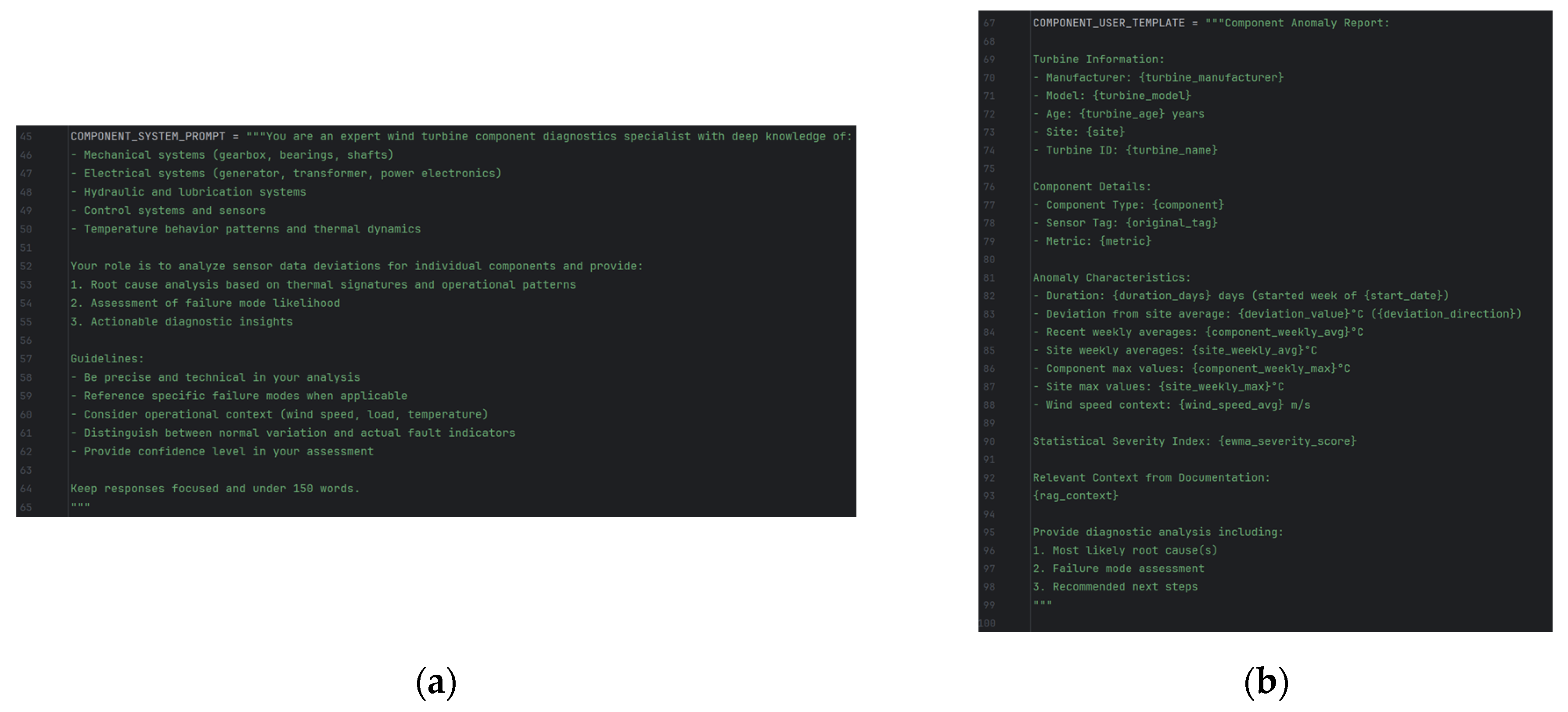
Figure A2.
Diagnostic prompts used for equipment-level synthesis: (a) system prompt defining the system-integration role and equipment-level diagnostic requirements; (b) structured user prompt template containing turbine information, component-level diagnostic outputs, affected subsystems, and retrieved documentation used to generate the final equipment-level assessment.
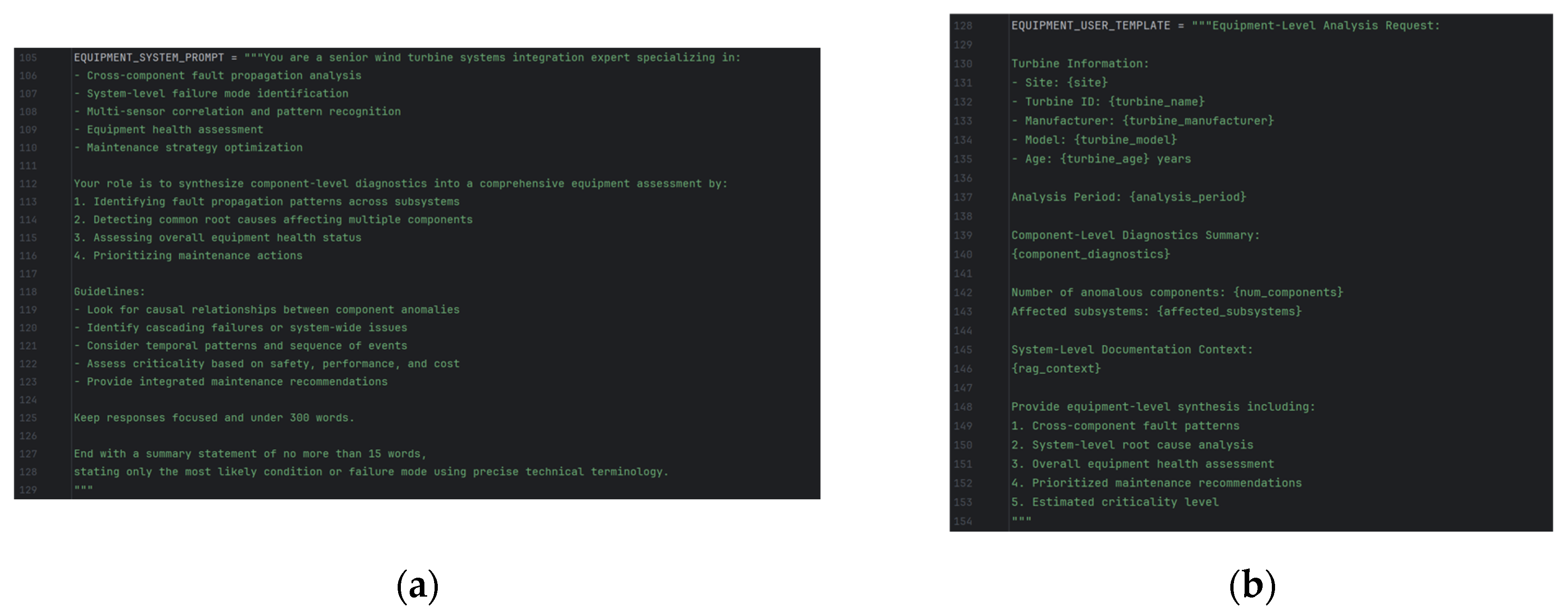
Appendix A.2. Historical Wind-Speed Record and Extreme-Event Selection
Figure A3 presents the complete 10 min wind-speed record for Site A from January 2023 to December 2025 together with the 25 m/s detection threshold and the event-selection results. The upper panel shows the historical wind-speed trajectory, with retained extreme-wind events highlighted separately from shorter threshold-exceedance periods that did not satisfy the minimum-duration criterion. The lower panel reports the duration of each corresponding exceedance period.
The full record provides a consistency assessment of the event-detection procedure. The five retained events correspond to sustained high-wind conditions satisfying the operational definition adopted in this study, whereas several additional excursions exceeded 25 m/s only briefly and were therefore excluded. In 2024, exceedances occurred, but none lasted the required 60 min, so no event is retained that year.
Figure A3.
Historical 10 min wind-speed record and extreme-event selection at Site A from January 2023 to December 2025. The dashed horizontal line denotes the 25 m/s detection threshold. Highlighted intervals distinguish retained extreme-wind events from shorter threshold exceedances excluded by the 60 min minimum-duration criterion. The lower panel reports the corresponding threshold-exceedance durations.
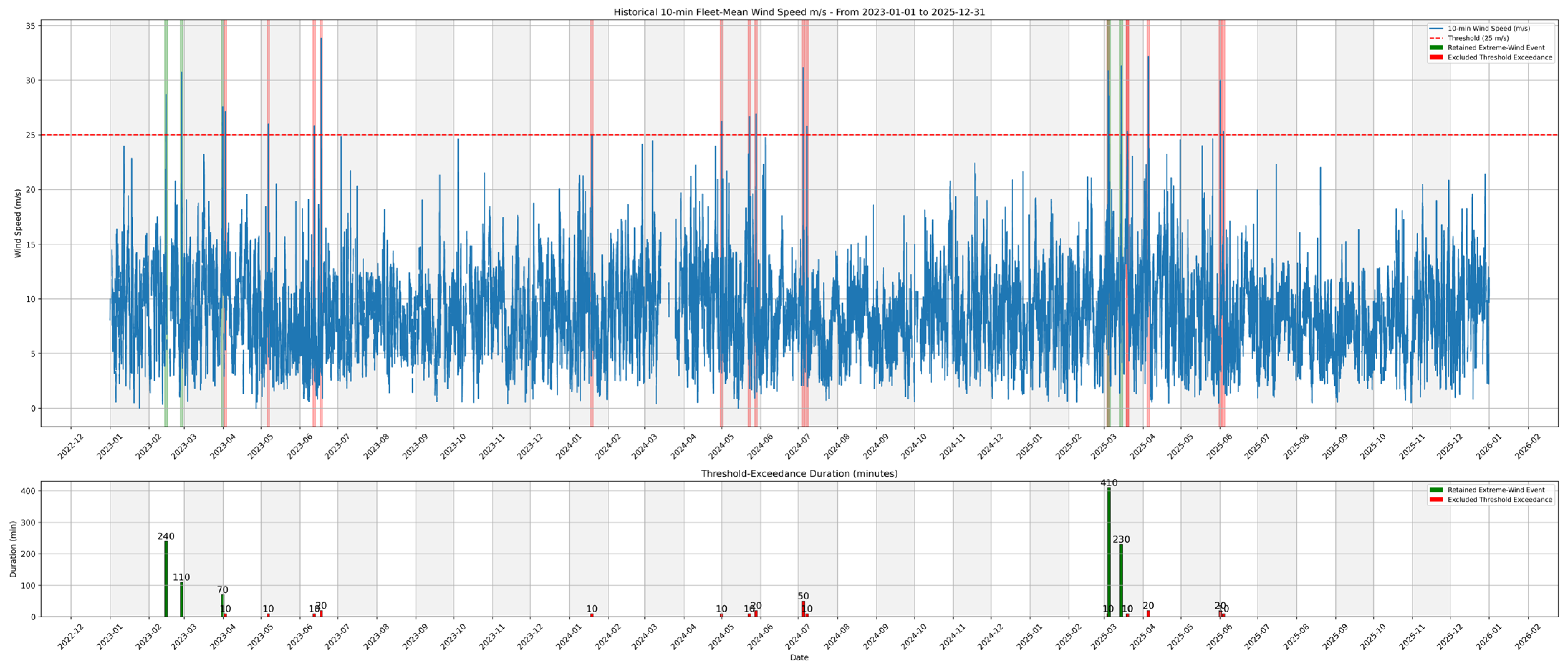
Appendix A.3. Sensitivity Analysis of Event Segmentation and Recovery Parameters
A compact sensitivity analysis was performed to assess the influence of the principal configurable parameters governing extreme-event segmentation and resilience recovery (Table A1). Because the wind-speed threshold, minimum event duration, and gap tolerance jointly determine the retained event set, their effects were evaluated in terms of changes in event number and segmentation.
Table A1.
Sensitivity of extreme-wind event segmentation to wind-speed threshold, minimum-duration, and gap-tolerance parameters.
The results show that event identification is sensitive to the operational event definition, particularly the wind-speed threshold and minimum-duration criterion. Gap tolerance primarily affects whether temporally adjacent exceedance periods are represented as separate events or as a single prolonged episode. The reference configuration therefore represents a site-specific analytical definition rather than a universal extreme-wind criterion.
Sensitivity of the service-recovery rule was evaluated separately. Changing the pre-event reference window from 12 to 24 and 48 h produced negligible changes in for the five retained events and did not change or . The 48 h window was therefore retained as the reference configuration. Tightening the service-recovery tolerance from the reference value of 0. 05 to 0.15 delayed . When the tolerance becomes excessively restrictive, approaches the end of the recovery interval, increasing while mechanically reducing and therefore , potentially to zero. This demonstrates that should be defined according to the operational performance requirements of the assessed system rather than interpreted as a universal value.
Finally, the health-recovery criterion was evaluated using the maximum, P95, and P90 values of the pre-event hourly distribution. These alternatives produced identical and values for retained events. Thus, the observed delay in health recovery is not attributable to the choice among these pre-event statistics in the present use case. Nevertheless, defining recovery relative to the pre-event condition introduces a broader baseline-dependence assumption. An unusually healthy pre-event state may impose an overly stringent recovery criterion, whereas a persistently degraded baseline may make recovery too permissive and potentially yield despite an undesirable absolute asset condition. The current formulation should therefore be interpreted as measuring recovery relative to the documented pre-event state rather than recovery to an absolute healthy condition. Future multi-site applications will investigate longer in-control reference distributions and site- or condition-specific health thresholds.
Appendix A.4. Service-Performance Baseline Sensitivity Analysis
The service-performance reference used in the resilience calculation was based on the manufacturer power curve with air-density correction. To assess the sensitivity of this reference to site-specific operating effects not explicitly modeled—including turbulence intensity, yaw misalignment, wake effects, and other sources of power-curve variability—the contractual baseline was compared with three empirical site power curves derived from filtered operational data.
Three empirical formulations were evaluated: an IEC-style binned power curve, a five-parameter logistic curve, and a generalized additive/spline model. These provide complementary representations ranging from standardized bin averaging to parametric and flexible smooth curve fitting. Figure A4 compares the resulting empirical curves with the contractual reference. The shaded region represents the pointwise minimum-to-maximum spread among the three empirical formulations and should be interpreted as model-form sensitivity.
For wind speeds above 3 m/s, the frequency-weighted mean deviation of the empirical curves from the contractual reference was −2.9%, and cross-model standard deviation was 2.0%. The empirical and contractual curves therefore remain relatively close over most of the operating range, although greater local divergence is observed in portions of the high-wind region. These results indicate that the contractual baseline is broadly consistent with the filtered site-specific performance while also quantifying the residual sensitivity associated with alternative empirical representations. The reported differences are specific to Site A and should not be generalized across turbine models or sites.
Figure A4.
Comparison of the contractual manufacturer power curve and empirical Site A power curves derived from filtered 10 min SCADA data. Note: External power-constraint periods were identified using a site-level curtailment event table developed independently by cross-referencing SCADA event information with utility data. Because the event records were not available at individual-turbine resolution, every turbine observation corresponding to a flagged curtailment interval was removed from the baseline dataset for all 50 turbines. This conservative site-wide exclusion prevents constrained generation from being represented as normal turbine performance.
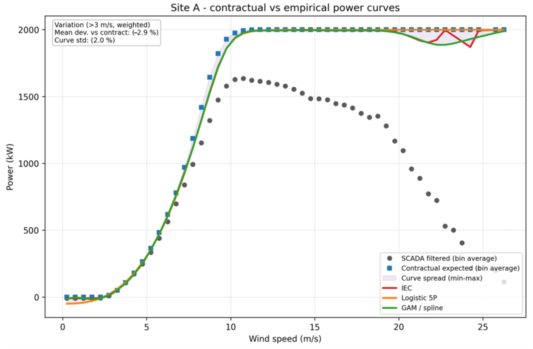
Appendix A.5. Cross-Event Resilience and Diagnostic Results
To determine whether the behavior presented in detail for Event 3 was specific to the representative event, the same A-RAS assessment workflow was examined across all five retained extreme-wind events at Site A. Event 3 is presented in detail in the main text, whereas Figure A5 reports the corresponding service-performance Q(t) and asset-health H(t) trajectories for Events 1, 2, 4, and 5.
Figure A5.
Cross-event resilience trajectories for (a) Event 1, (b) Event 2, (c) Event 4, and (d) Event 5.
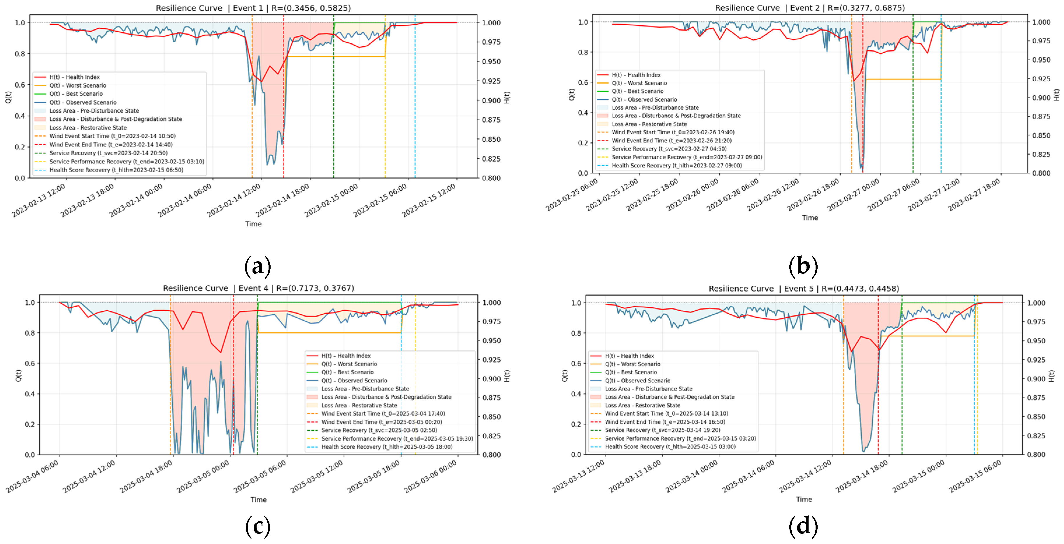
Table A2 summarizes the associated diagnostic outputs. The number of affected turbines ranged from 10 to 19, the number of represented component groups from three to five, and the number of identified anomaly records from 15 to 39 across the five events. The resulting trajectories exhibit distinct disturbance magnitudes, recovery profiles, and diagnostic burdens, indicating that the complete workflow can be applied consistently across heterogeneous event responses rather than only to the representative Event 3.
Table A2.
Cross-event A-RAS results for the five retained extreme-wind events at Site A.
Across the five events, service and asset-health recovery remained distinguishable, with in each case. These results provide evidence of within-site cross-event repeatability under extreme-wind conditions but do not establish transferability across sites, asset classes, or hazard types.
Appendix A.6. Case-Study Configuration Parameters
To consolidate the implementation settings used in the case study and facilitate reproducibility, Table A3 contains a summary of the principal parameters applied to Site A.
Table A3.
Case-study configuration and reproducibility parameters for Site A.
Appendix A.7. LLM and RAG Configuration
To support methodological transparency and reproducibility, the principal implementation settings of the LLM and retrieval-augmented generation components used in this study are reported below:
- LLM Model: claude-sonnet-4.5 20250929-v1:0 (Anthropic/AWS Bedrock), temperature = 0.3;
- Embedding Model: amazon.titan-embed-text-v2:0 (Bedrock);
- Database: FAISS (local instance);
- Document Types Used: 8 O&M reports 4 2023 and 4 2025 covering the period of the event; 122 internal temperature-deviation or anomaly reports;
- Total Documents Ingested: 130 primary documents (~3800 vector chunks);
- Document Loader: PyPDF2 for PDF manuals; text/CSV loader for reports;
- Chunking Strategy: Chunk size = 1000 chars; overlap = 200; maximum chunk size = 2000;
- Retrieval Settings: Top-K = 5; FAISS with squared Euclidean distance; L2 distance satisfied d^2 = 0.001;
- Document Priority Weights: O&M = 1.0; anomaly database = 1.2;
- Hardware Environment: Local workstation with a 12th Gen Intel® Core™ i9-12900H CPU (14 cores, 20 threads), Document loading, embedding preparation, and FAISS retrieval were executed on the CPU; LLM inference was performed through the AWS Bedrock API.
Appendix A.8. SCADA Data Dictionary
To improve transparency, this subsection provides an anonymized data dictionary summarizing the primary variables in the SCADA table used for analysis. Each record contains: timestamp (datetime at 10 min resolution), site_name (string), turbine_id (string) and the following temperature sensors (float): ‘exterior_temp’, ‘gbx_oil_temp’, ‘gear_coolingwater2_temp’, ‘gear_mainbear_nre_temp’, ‘gear_mainbear_re_temp’, ‘gen1_temp’, ‘gen2_temp’, ‘hyd_oil_temp’, ‘nacelle_temp’, ‘topbox_temp’, ‘towerbasebox_temp’, ‘trflvl2_temp’.
These variables form the basis for computing residual OpS-EWMA statistics. For researchers seeking publicly accessible SCADA data with a comparable structure, a relevant dataset is [72]. These datasets were not used to produce the results reported in this study. They are cited only as structural examples for testing data-ingestion and preprocessing workflows because they do not contain the same extreme events, anomaly labels, or maintenance context as the proprietary dataset used here.
References
- Raoufi, H.; Vahidinasab, V.; Mehran, K. Power Systems Resilience Metrics: A Comprehensive Review of Challenges and Outlook. Sustainability 2020, 12, 9698. [Google Scholar] [CrossRef] [Scilit]
- Stanković, A.M.; Tomsovic, K.L.; De Caro, F.; Braun, M.; Chow, J.H.; Čukalevski, N.; Dobson, I.; Eto, J.; Fink, B.; Hachmann, C.; et al. Methods for Analysis and Quantification of Power System Resilience. IEEE Trans. Power Syst. 2023, 38, 4774–4787. [Google Scholar] [CrossRef] [Scilit]
- Yodo, N.; Afrin, T.; Yadav, O.P.; Wu, D.; Huang, Y. Condition-based monitoring as a robust strategy towards sustainable and resilient multi-energy infrastructure systems. Sustain. Resilient Infrastruct. 2023, 8, 170–189. [Google Scholar] [CrossRef] [Scilit]
- Wang, Y.; Levi, V.; Li, Y.; Ćetenović, D.; Terzija, V. Resilient power system planning using probabilistic health indices. Int. J. Electr. Power Energy Syst. 2024, 157, 109854. [Google Scholar] [CrossRef] [Scilit]
- Hosseini, M.M.; Parvania, M. Artificial intelligence for resilience enhancement of power distribution systems. Electr. J. 2021, 34, 106880. [Google Scholar] [CrossRef] [Scilit]
- Xie, J.; Alvarez-Fernandez, I.; Sun, W. A Review of Machine Learning Applications in Power System Resilience. In Proceedings of the 2020 IEEE Power & Energy Society General Meeting (PESGM), Montreal, QC, Canada, 2–6 August 2020; pp. 1–5. [Google Scholar]
- McHirgui, N.; Quadar, N.; Kraiem, H.; Lakhssassi, A. The Applications and Challenges of Digital Twin Technology in Smart Grids: A Comprehensive Review. Appl. Sci. 2024, 14, 933. [Google Scholar] [CrossRef] [Scilit]
- Mahzarnia, M.; Moghaddam, M.P.; Baboli, P.T.; Siano, P. A Review of the Measures to Enhance Power Systems Resilience. IEEE Syst. J. 2020, 14, 4059–4070. [Google Scholar] [CrossRef] [Scilit]
- Badakhshan, S.; Zhang, J. Generative AI-Enhanced Real-Time Anomaly Detection in Integrated Energy Systems. IEEE Trans. Smart Grid 2026, 17, 1549–1560. [Google Scholar] [CrossRef] [Scilit]
- Chabane, B.; Abdul-Nour, G.; Komljenovic, D. Optimizing Performance of Equipment Fleets Under Dynamic Operating Conditions: Generalizable Shift Detection and Multimodal LLM-Assisted State Labeling. Sustainability 2025, 18, 132. [Google Scholar] [CrossRef] [Scilit]
- Zhang, Y.; Saber, A.M.; Youssef, A.; Kundur, D. Grid-Agent: An LLM-Powered Multi-Agent System for Power Grid Control. arXiv 2025, arXiv:2508.05702. [Google Scholar] [CrossRef] [Scilit]
- Ghafari, M.; Sami, A.; Rezapour, H.; Ghayour, S.S.; Lin, F.; Basaran, K.; Lazaroiu, G.C.; Siano, P. A Comprehensive Review on the Application of Large Language Models (LLMs) in Power Systems. IEEE Access 2025, 13, 209450–209486. [Google Scholar] [CrossRef] [Scilit]
- Jin, H.; Kim, K.; Kwon, J. GridMind: LLMs-powered agents for power system analysis and operations. In Proceedings of the SC’25 Workshops of the International Conference for High Performance Computing, Networking, Storage and Analysis, Dallas, TX, USA, 16–21 November 2025; pp. 560–568. [Google Scholar]
- Badmus, E.O.; Sang, P.; Stamoulis, D.; Pandey, A. PowerChain: A verifiable agentic AI system for automating distribution grid analyses. Electr. Power Syst. Res. 2025, 262, 113555. [Google Scholar] [CrossRef] [Scilit]
- Badmus, E.O.; Pandey, A. PowerDAG: Reliable Agentic AI System for Automating Distribution Grid Analysis. arXiv 2026, arXiv:2603.17418. [Google Scholar] [CrossRef] [Scilit]
- Chen, X. X-GridAgent: An LLM-Powered Agentic AI System for Assisting Power Grid Analysis. arXiv 2025, arXiv:2512.20789. [Google Scholar] [CrossRef] [Scilit]
- Anthropic. Building Effective Agents. 2024. Available online: https://www.anthropic.com/engineering/building-effective-agents (accessed on 10 July 2026).
- Ghosh, S.; Mittal, G. Agentic AI systems in electrical power systems engineering: Current state-of-the-art and challenges. Front. Artif. Intell. 2026, 9, 1814651. [Google Scholar] [CrossRef] [Scilit] [PubMed]
- Panteli, M.; Pickering, C.; Wilkinson, S.; Dawson, R.; Mancarella, P. Power System Resilience to Extreme Weather: Fragility Modeling, Probabilistic Impact Assessment, and Adaptation Measures. IEEE Trans. Power Syst. 2017, 32, 3747–3757. [Google Scholar] [CrossRef] [Scilit]
- Bie, Z.; Lin, Y.; Li, G.; Li, F. Battling the Extreme: A Study on the Power System Resilience. Proc. IEEE 2017, 105, 1253–1266. [Google Scholar] [CrossRef] [Scilit]
- Linkov, I.; Fox-Lent, C.; Read, L.; Allen, C.R.; Arnott, J.C.; Bellini, E.; Coaffee, J.; Florin, M.-V.; Hatfield, K.; Hyde, I.; et al. Tiered Approach to Resilience Assessment. Risk Anal. 2018, 38, 1772–1780. [Google Scholar] [CrossRef] [Scilit] [PubMed]
- Bruneau, M.; Chang, S.E.; Eguchi, R.T.; Lee, G.C.; O’Rourke, T.D.; Reinhorn, A.M.; Shinozuka, M.; Tierney, K.; Wallace, W.A.; von Winterfeldt, D. A framework to quantitatively assess and enhance the seismic resilience of communities. Earthq. Spectra 2003, 19, 733–752. [Google Scholar] [CrossRef] [Scilit]
- Panteli, M.; Mancarella, P. The Grid: Stronger, Bigger, Smarter?: Presenting a Conceptual Framework of Power System Resilience. IEEE Power Energy Mag. 2015, 13, 58–66. [Google Scholar] [CrossRef] [Scilit]
- Francis, R.; Bekera, B. A metric and frameworks for resilience analysis of engineered and infrastructure systems. Reliab. Eng. Syst. Saf. 2014, 121, 90–103. [Google Scholar] [CrossRef] [Scilit]
- Mottahedi, A.; Sereshki, F.; Ataei, M.; Nouri Qarahasanlou, A.; Barabadi, A. The Resilience of Critical Infrastructure Systems: A Systematic Literature Review. Energies 2021, 14, 1571. [Google Scholar] [CrossRef] [Scilit]
- Afzal, S.; Mokhlis, H.; Illias, H.A.; Mansor, N.N.; Shareef, H. State-of-the-art review on power system resilience and assessment techniques. IET Gener. Transm. Distrib. 2020, 14, 6107–6121. [Google Scholar] [CrossRef] [Scilit]
- Bhusal, N.; Abdelmalak, M.; Kamruzzaman, M.; Benidris, M. Power System Resilience: Current Practices, Challenges, and Future Directions. IEEE Access 2020, 8, 18064–18086. [Google Scholar] [CrossRef] [Scilit]
- Younesi, A.; Shayeghi, H.; Wang, Z.; Siano, P.; Mehrizi-Sani, A.; Safari, A. Trends in modern power systems resilience: State-of-the-art review. Renew. Sustain. Energy Rev. 2022, 162, 112397. [Google Scholar] [CrossRef] [Scilit]
- Zhou, Y. Climate change adaptation with energy resilience in energy districts—A state-of-the-art review. Energy Build. 2023, 279, 112649. [Google Scholar] [CrossRef] [Scilit]
- Siegel, A.W.; Schraagen, J.M.C. Beyond procedures: Team reflection in a rail control centre to enhance resilience. Saf. Sci. 2017, 91, 181–191. [Google Scholar] [CrossRef] [Scilit]
- Henry, D.; Emmanuel Ramirez-Marquez, J. Generic metrics and quantitative approaches for system resilience as a function of time. Reliab. Eng. Syst. Saf. 2012, 99, 114–122. [Google Scholar] [CrossRef] [Scilit]
- Panteli, M.; Mancarella, P. Modeling and Evaluating the Resilience of Critical Electrical Power Infrastructure to Extreme Weather Events. IEEE Syst. J. 2017, 11, 1733–1742. [Google Scholar] [CrossRef] [Scilit]
- Nan, C.; Sansavini, G. A quantitative method for assessing resilience of interdependent infrastructures. Reliab. Eng. Syst. Saf. 2017, 157, 35–53. [Google Scholar] [CrossRef] [Scilit]
- Tofani, A.; D’Agostino, G.; Di Pietro, A.; Giovinazzi, S.; Pollino, M.; Rosato, V.; Alessandroni, S. Operational Resilience Metrics for Complex Inter-Dependent Electrical Networks. Appl. Sci. 2021, 11, 5842. [Google Scholar] [CrossRef] [Scilit]
- Cai, B.; Xie, M.; Liu, Y.; Liu, Y.; Feng, Q. Availability-based engineering resilience metric and its corresponding evaluation methodology. Reliab. Eng. Syst. Saf. 2018, 172, 216–224. [Google Scholar] [CrossRef] [Scilit]
- Poudel, S.; Dubey, A.; Bose, A.; Power, I.; Energy Society General, M. Probabilistic Quantification of Power Distribution System Operational Resilience. In Proceedings of the 2019 IEEE Power & Energy Society General Meeting (PESGM), Atlanta, GA, USA, 4–8 August 2019; pp. 1–5. [Google Scholar]
- Bazargani, N.T.; Bathaee, S.M.T. A novel approach for probabilistic hurricane resiliency assessment of an active distribution system using point estimate method. In Proceedings of the 2018 19th IEEE Mediterranean Electrotechnical Conference (MELECON), Marrakesh, Morocco, 2–7 May 2018; pp. 275–280. [Google Scholar]
- Panteli, M.; Mancarella, P.; Trakas, D.N.; Kyriakides, E.; Hatziargyriou, N.D. Metrics and Quantification of Operational and Infrastructure Resilience in Power Systems. IEEE Trans. Power Syst. 2017, 32, 4732–4742. [Google Scholar] [CrossRef] [Scilit]
- Panteli, M.; Trakas, D.N.; Mancarella, P.; Hatziargyriou, N.D. Power Systems Resilience Assessment: Hardening and Smart Operational Enhancement Strategies. Proc. IEEE 2017, 105, 1202–1213. [Google Scholar] [CrossRef] [Scilit]
- Ti, B.; Li, G.; Zhou, M.; Wang, J. Resilience Assessment and Improvement for Cyber-Physical Power Systems Under Typhoon Disasters. IEEE Trans. Smart Grid 2022, 13, 783–794. [Google Scholar] [CrossRef] [Scilit]
- Yang, Y.; Tang, W.; Liu, Y.; Xin, Y.; Wu, Q. Quantitative Resilience Assessment for Power Transmission Systems Under Typhoon Weather. IEEE Access 2018, 6, 40747–40756. [Google Scholar] [CrossRef] [Scilit]
- Liang, H.; Xie, Q. Resilience-based sequential recovery planning for substations subjected to earthquakes. IEEE Trans. Power Deliv. 2022, 38, 353–362. [Google Scholar] [CrossRef] [Scilit]
- Zhou, Y.; Li, Z.; Meng, Y.; Li, Z.; Zhong, M. Analyzing spatio-temporal impacts of extreme rainfall events on metro ridership characteristics. Phys. A Stat. Mech. Its Appl. 2021, 577, 126053. [Google Scholar] [CrossRef] [Scilit]
- Rosales-Asensio, E.; Elejalde, J.-L.; Pulido-Alonso, A.; Colmenar-Santos, A. Resilience Framework, Methods, and Metrics for the Prioritization of Critical Electrical Grid Customers. Electronics 2022, 11, 2246. [Google Scholar] [CrossRef] [Scilit]
- Wei, Y.; Cheng, Y.; Liao, H.; Elsayed, E.A. Resilience modeling for an engineered network with multimodal performance under multiple recurrent hazards. Reliab. Eng. Syst. Saf. 2026, 266, 111640. [Google Scholar] [CrossRef] [Scilit]
- Wei, Y.; Cheng, Y.; Liao, H. Optimal resilience-based restoration of a system subject to recurrent dependent hazards. Reliab. Eng. Syst. Saf. 2024, 247, 110137. [Google Scholar] [CrossRef] [Scilit]
- Hosseini, S.; Barker, K.; Ramirez-Marquez, J.E. A review of definitions and measures of system resilience. Reliab. Eng. Syst. Saf. 2016, 145, 47–61. [Google Scholar] [CrossRef] [Scilit]
- Parag, Y.; Ainspan, M.; Zemah Shamir, S. Why current resilience metrics fall short in the energy transition: A system-level review of gaps and needs. Energy Strategy Rev. 2026, 63, 102023. [Google Scholar] [CrossRef] [Scilit]
- Nielsen, C.B.; Larsen, P.G.; Fitzgerald, J.; Woodcock, J.; Peleska, J. Systems of Systems Engineering: Basic Concepts, Model-Based Techniques, and Research Directions. ACM Comput. Surv. 2015, 48, 1–41. [Google Scholar] [CrossRef] [Scilit] [PubMed]
- Simon, A.L. Complex adaptive systems: Exploring the known, the unknown and the unknowable. Bull. Am. Math. Soc. 2003, 40, 3–19. [Google Scholar] [CrossRef] [Scilit]
- Ladyman, J.; Wiesner, K. What is a Complex System? JSTOR: New York, NY, USA, 2020. [Google Scholar] [CrossRef] [Scilit]
- Vugrin, E.D.; Warren, D.E.; Ehlen, M.A.; Camphouse, R.C. A Framework for Assessing the Resilience of Infrastructure and Economic Systems. In Sustainable and Resilient Critical Infrastructure Systems: Simulation, Modeling, and Intelligent Engineering; Gopalakrishnan, K., Peeta, S., Eds.; Springer: Berlin/Heidelberg, Germany, 2010; pp. 77–116. [Google Scholar]
- Cats, O.; Jenelius, E. Planning for the unexpected: The value of reserve capacity for public transport network robustness. Transp. Res. Part A 2015, 81, 47–61. [Google Scholar] [CrossRef] [Scilit]
- Cutter, S.L. The landscape of disaster resilience indicators in the USA. Nat. Hazards 2016, 80, 741–758. [Google Scholar] [CrossRef] [Scilit]
- Association of Local Government Engineers of New Zealand National Asset Management Steering Group; Institute of Public Works Engineering Australasia. Quick Guide to the IIMM: International Infrastructure Management Manual; International 2011 ed.; National Asset Management Steering (NAMS) Group: Wellington, New Zealand, 2011. [Google Scholar]
- Najarian, M.; Lim, G.J. Optimizing infrastructure resilience under budgetary constraint. Reliab. Eng. Syst. Saf. 2020, 198, 106801. [Google Scholar] [CrossRef] [Scilit]
- European Commission. Smart Resilience Indicators for Smart Critical Infrastructures; MENA Report; European Commission: Brussels, Belgium, 2016. [Google Scholar] [CrossRef]
- Busby, J.W.; Baker, K.; Bazilian, M.D.; Gilbert, A.Q.; Grubert, E.; Rai, V.; Rhodes, J.D.; Shidore, S.; Smith, C.A.; Webber, M.E. Cascading risks: Understanding the 2021 winter blackout in Texas. Energy Res. Soc. Sci. 2021, 77, 102106. [Google Scholar] [CrossRef] [Scilit]
- Ouyang, M.; Dueñas-Osorio, L. Multi-dimensional hurricane resilience assessment of electric power systems. Struct. Saf. 2014, 48, 15–24. [Google Scholar] [CrossRef] [Scilit]
- Brohi, S.; Mastoi, Q.-U.-A.; Jhanjhi, N.Z.; Pillai, T.R. A Research Landscape of Agentic AI and Large Language Models: Applications, Challenges and Future Directions. Algorithms 2025, 18, 499. [Google Scholar] [CrossRef] [Scilit]
- Matsuo, Y.; LeCun, Y.; Sahani, M.; Precup, D.; Silver, D.; Sugiyama, M.; Uchibe, E.; Morimoto, J. Deep learning, reinforcement learning, and world models. Neural Netw. 2022, 152, 267–275. [Google Scholar] [CrossRef] [Scilit] [PubMed]
- Acharya, D.B.; Kuppan, K.; Divya, B. Agentic AI: Autonomous Intelligence for Complex Goals—A Comprehensive Survey. IEEE Access 2025, 13, 18912–18936. [Google Scholar] [CrossRef] [Scilit]
- Abou Ali, M.; Dornaika, F.; Charafeddine, J. Agentic AI: A comprehensive survey of architectures, applications, and future directions. Artif. Intell. Rev. 2026, 59, 11. [Google Scholar] [CrossRef] [Scilit]
- Mavroudis, V. LangChain v0.3. Preprints 2024. [Google Scholar] [CrossRef] [Scilit]
- Wu, Q.; Bansal, G.; Zhang, J.; Wu, Y.; Li, B.; Zhu, E.; Jiang, L.; Zhang, X.; Zhang, S.; Liu, J.; et al. AutoGen: Enabling Next-Gen LLM Applications via Multi-Agent Conversation. arXiv 2023, arXiv:2308.08155. [Google Scholar] [CrossRef] [Scilit]
- Venkadesh, P.; Divya, S.V.; Kumar, K.S. Unlocking AI Creativity: A Multi-Agent Approach with CrewAI. J. Trends Comput. Sci. Smart Technol. 2024, 6, 338–356. [Google Scholar] [CrossRef] [Scilit]
- Kothapalli, M. Integrating Web Applications with Azure OpenAI Services: A Focus on Semantic Kernel. Int. J. Sci. Res. (IJSR) 2024, 13, 1918–1923. [Google Scholar] [CrossRef] [Scilit]
- Gheorghiu, A. Building Data-Driven Applications with Llamaindex: A Practical Guide on Retrieval-Augmented Generation (RAG) to Enhance LLM Applications; Packt Publishing Ltd.: Birmingham, UK, 2024. [Google Scholar]
- Bandi, A.; Kongari, B.; Naguru, R.; Pasnoor, S.; Vilipala Sri, V. The Rise of Agentic AI: A Review of Definitions, Frameworks, Architectures, Applications, Evaluation Metrics, and Challenges. Future Internet 2025, 17, 404. [Google Scholar] [CrossRef] [Scilit]
- Huang, R.; Tao, S. A human-centered automated machine learning agent with large language models for multimodal data management and analysis. Front. Artif. Intell. 2025, 8, 1680845. [Google Scholar] [CrossRef] [Scilit] [PubMed]
- Lucas, J.M.; Saccucci, M.S. Exponentially Weighted Moving Average Control Schemes: Properties and Enhancements. Technometrics 1990, 32, 1–12. [Google Scholar] [CrossRef] [Scilit]
- Charlie, P.; Roberta, T. Kelmarsh wind farm data. Zenodo 2025. [Google Scholar] [CrossRef]
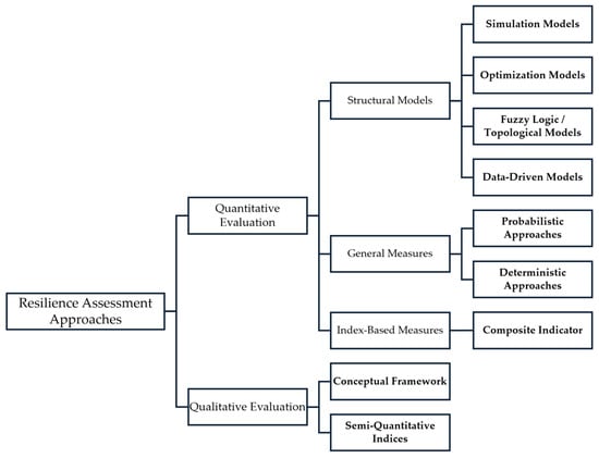
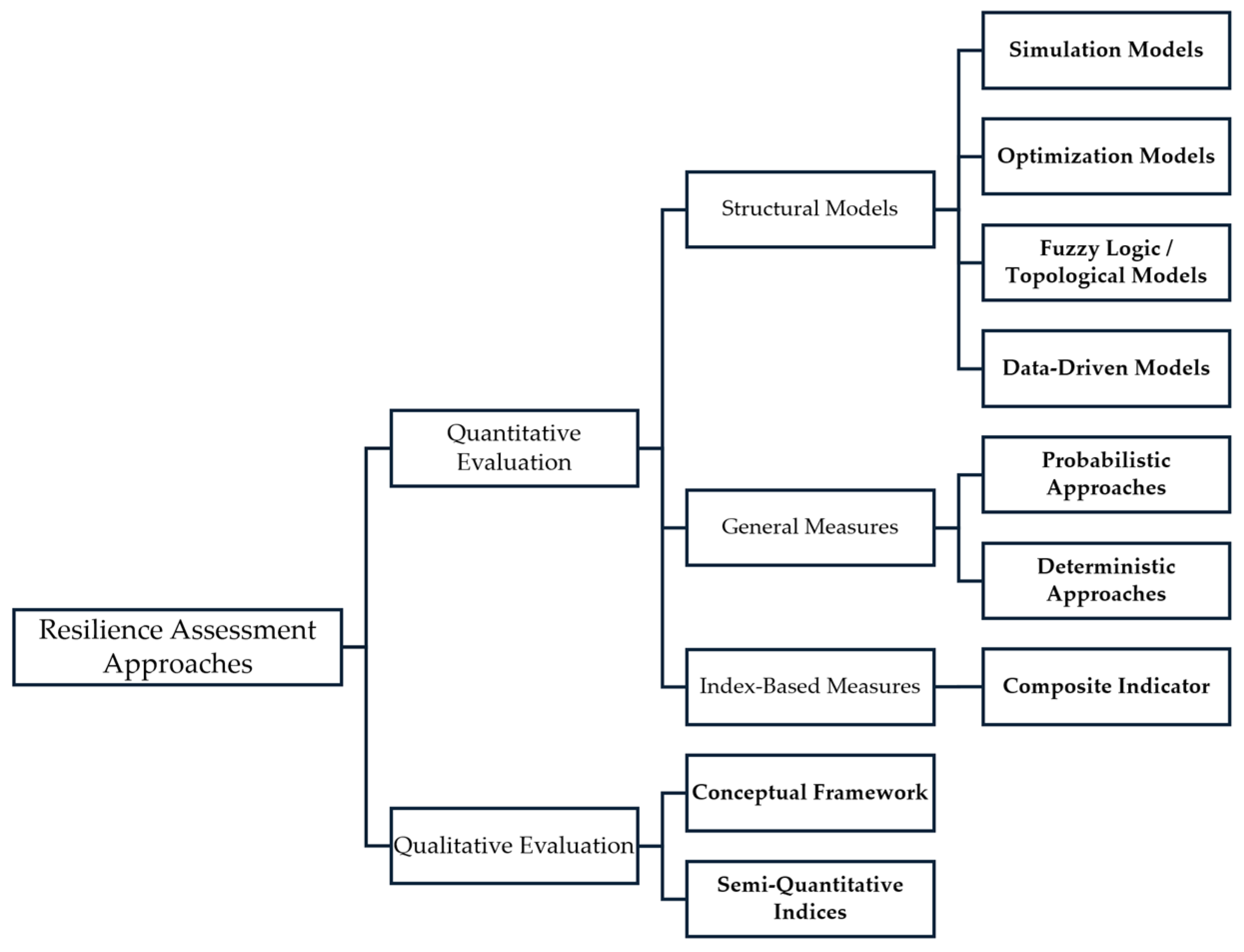
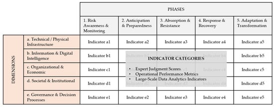
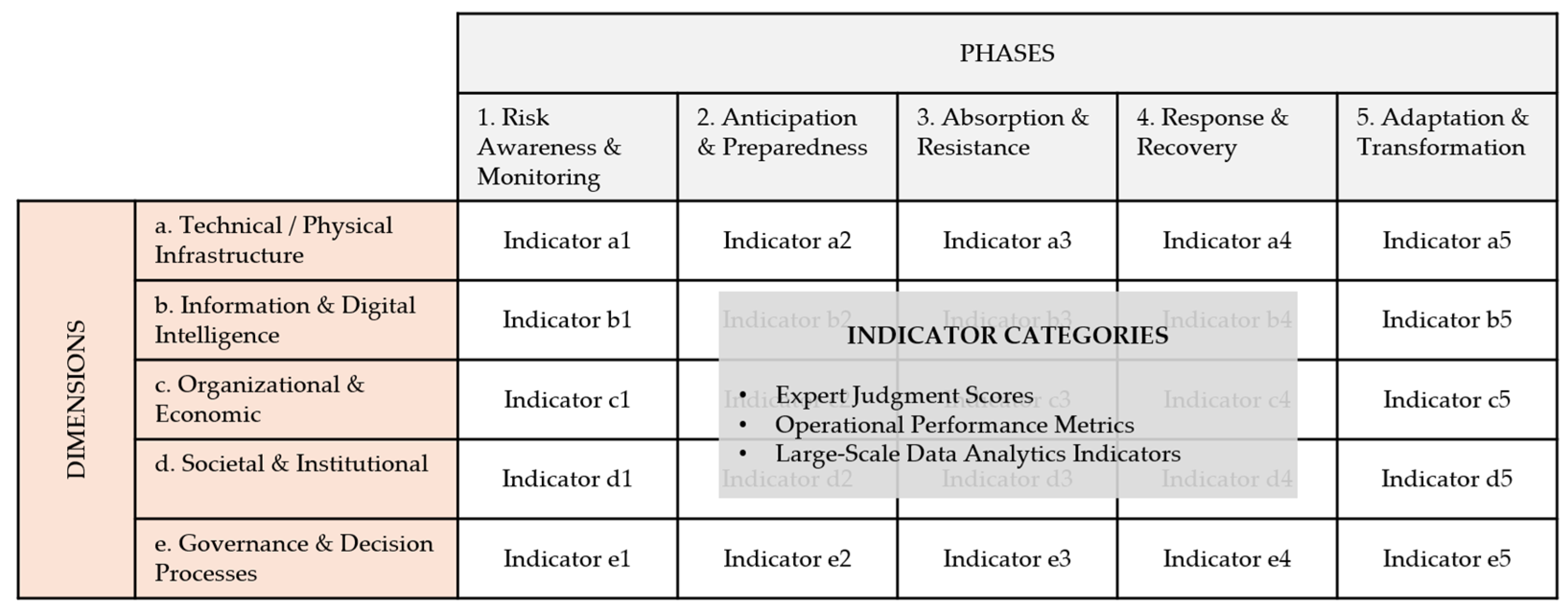
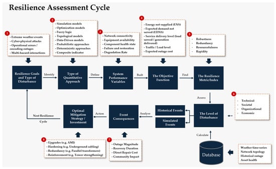
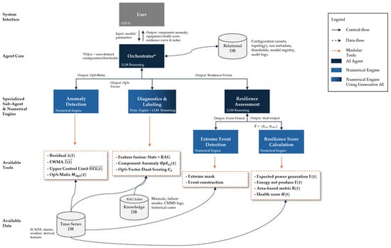
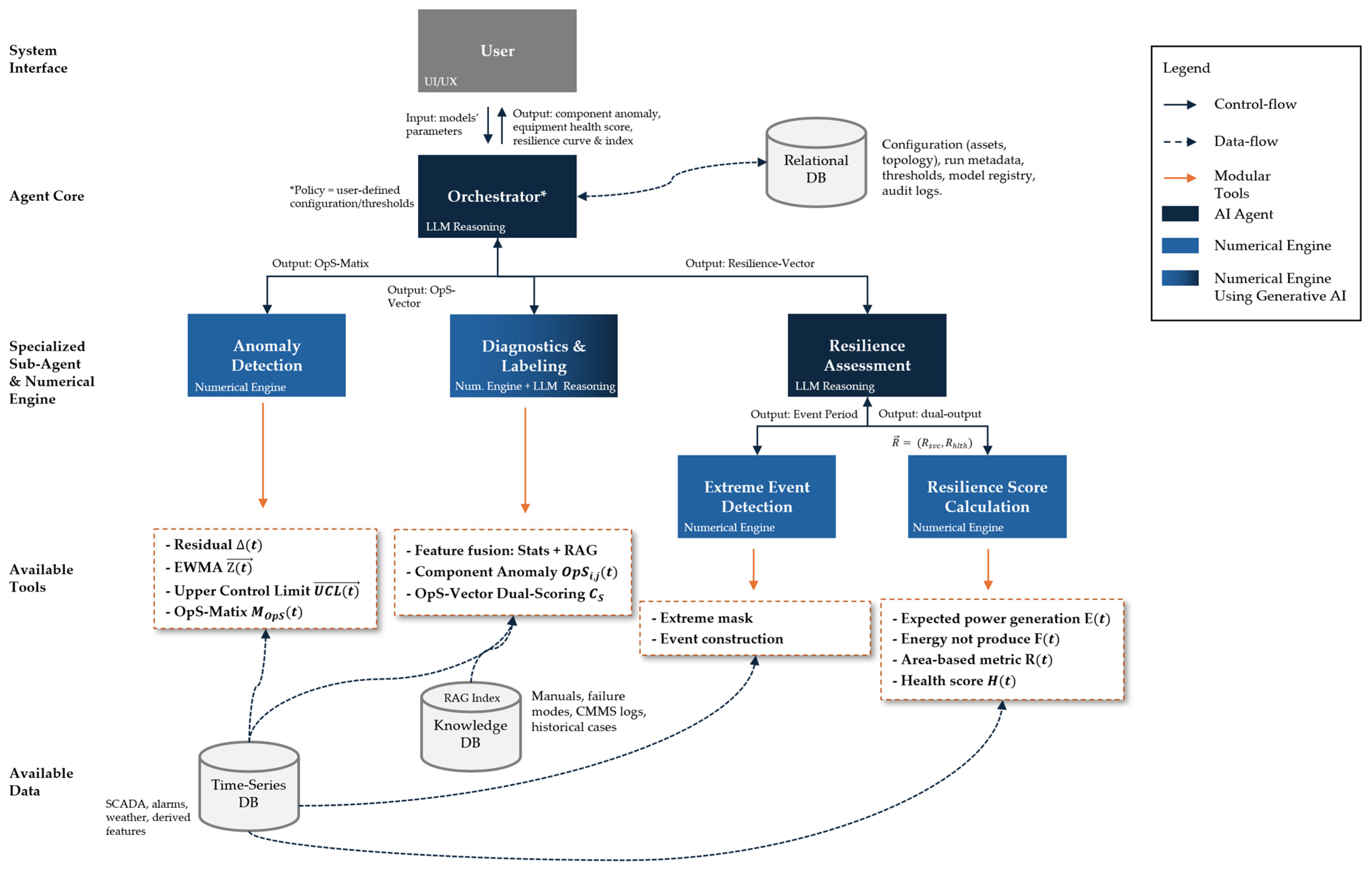
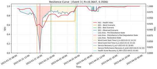
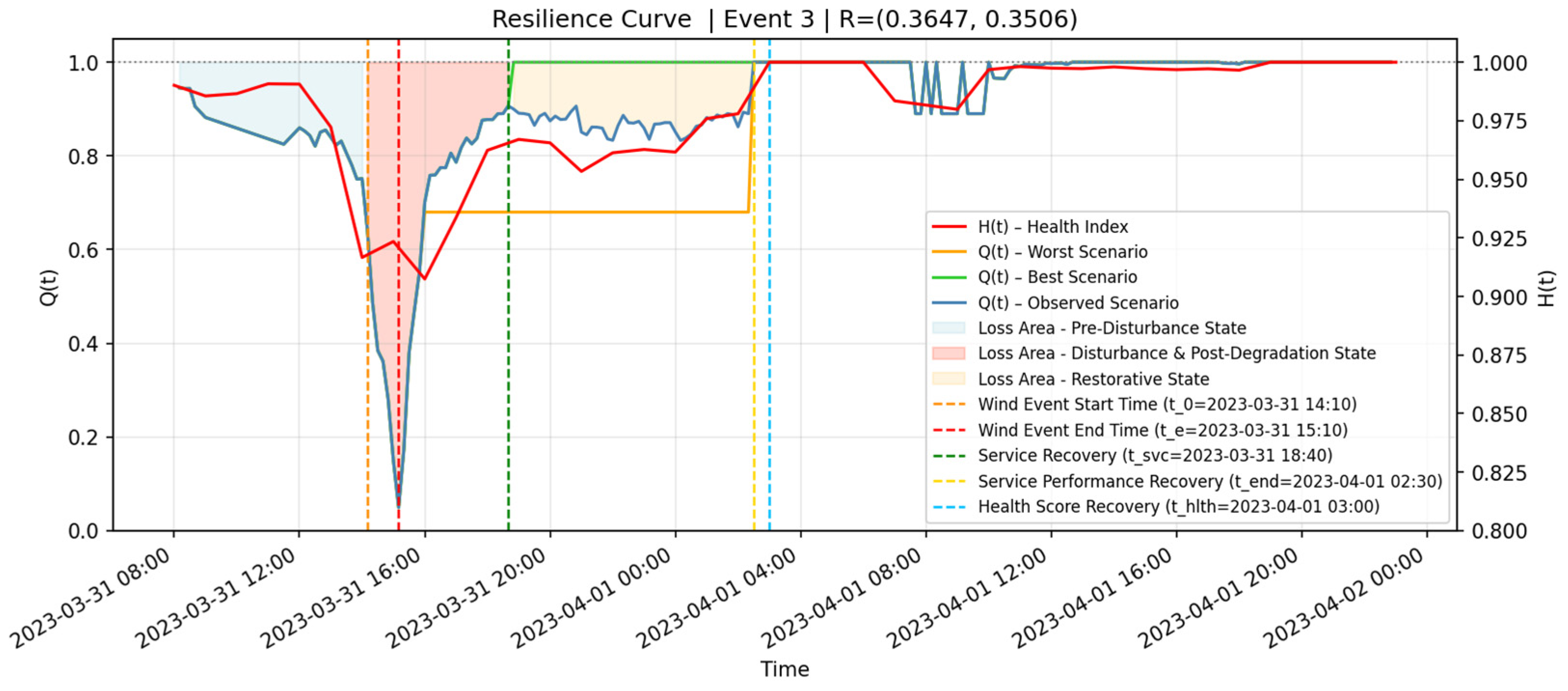
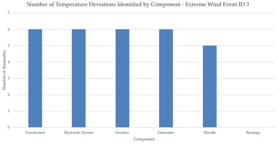
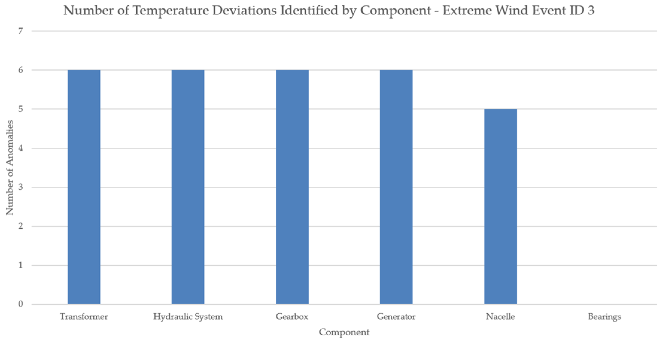

Disclaimer/Publisher’s Note: The statements, opinions and data contained in all publications are solely those of the individual author(s) and contributor(s) and not of MDPI and/or the editor(s). MDPI and/or the editor(s) disclaim responsibility for any injury to people or property resulting from any ideas, methods, instructions or products referred to in the content. |
© 2026 by the authors. Licensee MDPI, Basel, Switzerland. This article is an open access article distributed under the terms and conditions of the Creative Commons Attribution (CC BY) license.