Virtual Synchronous Generator Multi-Parameter Cooperative Adaptive Control Based on a Fuzzy and Soft Actor–Critic Fusion Framework

Abstract

To address the issue that distributed renewable energy grid-connected Virtual Synchronous Generator (VSG) systems are prone to significant power and frequency fluctuations under changing operating conditions, this paper proposes a multi-parameter coordinated control strategy for VSGs based on a fusion framework of fuzzy logic and the Soft Actor–Critic (SAC) algorithm, termed Improved SAC-based Virtual Synchronous Generator control (ISAC-VSG). First, the method uses fuzzy logic to map the frequency deviation and its rate of change into a five-dimensional membership vector, which characterizes the uncertainty and nonlinear features during the transient process, enabling segmented policy optimization for different transient regions. Second, a stage-based guidance mechanism is introduced into the reward function to balance the agent’s exploration and stability, thereby improving the reliability of the policy. Finally, the action space is expanded from inertia–damping to the coordinated regulation of inertia, damping, and active power droop coefficient, achieving multi-parameter dynamic optimization. MATLAB/Simulink R2022b simulation results indicate that, compared with the traditional SAC-VSG and DDPG-VSG method, the proposed strategy can reduce the maximum frequency overshoot by up to 29.6% and shorten the settling time by approximately 15.6% under typical operating conditions such as load step changes and grid phase disturbances. It demonstrates superior frequency oscillation suppression capability and system robustness, verifying the effectiveness and application potential of the proposed method in high-penetration renewable energy power systems.

1. Introduction

In the context of the “dual-high” era—characterized by a high proportion of renewable energy and highly volatile loads—distributed energy sources such as wind and solar power have seen widespread deployment [1,2,3]. Since these energy sources are typically integrated into the grid through power electronic converters, large-scale grid connection results in low-inertia and weak-damping characteristics, posing severe challenges to frequency stability and dynamic regulation capability of the power system [4]. To enhance the system’s dynamic support capability, researchers have proposed the Virtual Synchronous Generator (VSG) control technology, which emulates the inertia, electromagnetic, and damping characteristics of a synchronous generator (SG) within an inverter. This allows the system to possess adjustable virtual inertia and damping, thereby effectively improving frequency stability and dynamic response quality under high renewable penetration scenarios [5]. However, while providing inertia support, VSGs also inherit the low-frequency oscillation risks of SGs. Compared with traditional SGs, VSG parameters are adjustable, and the dynamic response performance can be enhanced by tuning the virtual inertia J, damping coefficient D, and active power droop coefficient $D_p$ [6]. If parameter selection is inappropriate, both frequency and power oscillations may be amplified. Therefore, achieving adaptive optimal parameter tuning under complex disturbances is of great research significance [7].

Existing research on adaptive control of VSG parameters can be categorized into the following types. The first category includes mechanism-model-based adaptive adjustment methods, which rely on accurate mathematical models of the system and construct adjustment laws through small-signal analysis, linear techniques, or model predictive control [8,9]. Reference [10] adopts current model predictive control for adaptive tuning of VSG parameters, resolving the contradiction between dynamic response and steady-state accuracy in traditional control. References [11,12] apply a linear quadratic regulator (LQR) to design adaptive tuning rules for virtual inertia and damping. Although these methods offer strong theoretical rigor, they require high model accuracy and parameter accessibility, making them difficult to apply in high-renewable systems with inherent uncertainties and nonlinearities [13].

The second category consists of experience-based parameter adjustment strategies that do not require complex system modeling. Reference [14] proposes a bang–bang adaptive control strategy that adaptively selects virtual inertia and damping based on frequency deviation and its rate of change. In [15], a controller combining fuzzy logic and a differential algorithm is used to adjust virtual inertia and damping, improving frequency stability in low-inertia microgrids with high renewable penetration. Reference [16] eliminates the need for precise mathematical modeling through expert knowledge and system measurement data, enabling the controller to adjust the virtual inertia parameter of the VSG. However, such methods rely heavily on thresholds and rule design, making it difficult to achieve robust performance and fast dynamics under complex disturbances.

The third category comprises intelligent optimization and data-driven strategy-learning approaches. References [17,18,19] use intelligent optimization algorithms such as particle swarm optimization and genetic algorithms for VSG parameter tuning, but they still depend on accurate modeling. In recent years, data-driven reinforcement learning (RL) methods have been introduced into VSG parameter coordination control and have demonstrated strong performance in model-free scenarios. For example, reference [20] applies Q-learning to VSG parameter tuning but only outputs a one-dimensional action—the virtual inertia J—and the reward function only considers frequency deviation. Although this improves dynamic frequency and active power response to some extent, algorithm efficiency deteriorates significantly as state and action dimensions increase. To address this, reference [21] proposes a DQN algorithm that uses a neural network to replace the Q-table in Q-learning for handling continuous states, with virtual inertia J and damping D set as discrete action space elements. Reference [22] adopts the DDPG algorithm to simultaneously adjust J and D in continuous action space, achieving better dynamic frequency performance. Reference [23] applies VSG control to modular multilevel converter (MMC) structures and uses the TD3 algorithm to adjust virtual inertia J, damping D, and voltage reference E.

Reference [24] further verifies the superiority of the Soft Actor–Critic (SAC) algorithm over other algorithms in VSG parameter adaptive control, demonstrating its effectiveness in suppressing power and frequency oscillations and shortening stabilization time. However, reference [20,21,22,23,24] typically limit their action space to the adjustment of only the virtual inertia J and damping coefficient D, failing to incorporate the active power droop coefficient $D_p$, which also significantly influences system dynamic characteristics into a framework for real-time cooperative optimization (see analysis in Section 2.2). This limitation results in insufficient flexibility for parameter adjustment under complex disturbances, thereby restricting further improvement of the system’s transient performance.

Building upon the aforementioned issues, this paper selects the Soft Actor–Critic (SAC) reinforcement learning algorithm as the foundational framework to investigate optimal VSG parameter regulation. The SAC algorithm encourages policy exploration through an entropy regularization term, demonstrating exceptional sample efficiency and training stability in stochastic environments [25].

The main contributions of this paper are as follows.

• A parameter adaptive control framework combining fuzzy logic and the Soft Actor–Critic (SAC) algorithm is proposed. By dividing the VSG operation process into different transient regions and constructing a state-cognition vector based on fuzzy membership, the controller can perform more targeted policy optimization for different transient characteristics.
• A reward-design mechanism that integrates transient-region guidance and autonomous exploration is developed. This method applies expert-experience-based action limiting and guidance according to different transient regions of the VSG system, improving SAC-VSG training stability while ensuring system safety.
• Beyond traditional SAC-VSG strategies that focus only on virtual inertia and damping, this work further investigates the influence of active power droop coefficient perturbation on VSG transient performance. An ISAC-VSG multi-parameter coordinated control strategy is proposed to enhance transient performance and robustness.

The rest of this paper is organized as follows: Section 2 introduces the basic VSG model, system performance analysis, and parameter tuning. Section 3 presents the improved SAC-VSG multi-parameter coordinated control strategy. Section 4 verifies the effectiveness of the proposed method using MATLAB/Simulink simulations. Section 5 provides conclusions and perspectives for future work.

2. VSG Fundamental Model and System Performance Parameter Analysis and Design

2.1. Fundamental Mathematical Model of VSG

The introduction of Virtual Synchronous Generator (VSG) control in grid-connected inverters aims to emulate the inertia and damping characteristics of synchronous generators (SGs), thereby enabling primary frequency regulation capability. A conventional SG can be described by a second-order model. Assuming the number of pole pairs is one, the equivalent rotor mechanical equation of a VSG can be expressed as A conventional SG can be described by a second-order model. Assuming the number of pole pairs is one, the equivalent rotor mechanical equation of a VSG can be expressed as

$$J{\displaystyle \frac{d\omega }{dt}}={\displaystyle \frac{P_m}{{\omega }_0}}-{\displaystyle \frac{P_e}{{\omega }_0}}-D(\omega -{\omega }_0)$$

(1)

where J and D denote the virtual inertia and damping coefficient, respectively; $\omega$ and ${\omega }_0$ represent the VSG output and nominal angular frequencies; $P_m$ and $P_e$ are the mechanical and electromagnetic powers of the VSG, and $P_{ref}$ is the active power reference.

The active power reference is typically adjusted through a droop control relationship as

$$P_{\mathrm{m}}=P_{ref}+D_p(w_0-w)$$

(2)

where $D_p$ is the active power droop coefficient. Combining (1) and (2) yields

$$J{\displaystyle \frac{dw}{dt}}={\displaystyle \frac{P_{ref}-P_e+D_p(w_0-w)}{w_0}}-D(\omega -{\omega }_0)$$

(3)

which forms the core dynamic equation of the VSG control system.

2.2. Influence of Parameter Perturbations on Grid-Connected VSG Performance

Since the impedance between the inverter output voltage and the grid voltage is generally inductive ($X\gg R$), the active and reactive power control loops can be approximately decoupled. Based on power flow theory, the active power injected into the grid can be expressed as

$$P_e={\displaystyle \frac{3E{U}_g}{X}}sin\delta$$

(4)

where

$$\delta =\int (w-w_g)dt$$

(5)

$U_g$ and ${\omega }_g$ are the RMS phase voltage and angular frequency of the grid, and E is the inverter output RMS voltage. For small-signal analysis, assuming $sin\delta \approx \delta$, a small-signal model of the VSG active power–frequency control loop can be established as

$$\left\{\begin{array}{c}{\displaystyle \frac{d(\Delta w)}{dt}}=-\left({\displaystyle \frac{D_p}{J{w}_0}}+{\displaystyle \frac{D}{J}}\right)\Delta w-{\displaystyle \frac{\Delta P_e}{J{w}_0}}\hfill \\ {\displaystyle \frac{d(\Delta \delta )}{dt}}=\Delta w\hfill \end{array}\right.$$

(6)

where $\Delta \omega$, $\Delta P_e$, and $\Delta \delta$ represent small perturbations of frequency, power, and power angle, respectively. According (6), the state-space representation of the VSG active power dynamics is

$$\left[\begin{array}{c}\Delta \dot{\delta }\\ \Delta \dot{w}\end{array}\right]=\left[\begin{array}{cc}0& 1\\ -{\displaystyle \frac{K_p}{J{w}_0}}& -{\displaystyle \frac{D_p}{J{w}_0}}-{\displaystyle \frac{D}{J}}\end{array}\right]\left[\begin{array}{c}\Delta \delta \\ \Delta w\end{array}\right]$$

(7)

and its eigenvalues [26] are

$$P_{1,2}=-{\displaystyle \frac{(D_p+D{w}_0)}{2J{w}_0}}\pm \sqrt{{\left({\displaystyle \frac{D_p+D{w}_0}{2J{w}_0}}\right)}^2-{\displaystyle \frac{K_p}{J{w}_0}}}$$

(8)

where $K_p={\displaystyle \frac{3U_{\mathrm{ref}}E}{X}}$, $U_{\mathrm{ref}}$ is the reference phase voltage, and X represents the equivalent impedance of the VSG.

The parameter values used for the single-machine grid-connected VSG system are listed in Table 1. According to Lyapunov’s first method, the system is stable when all eigenvalues have negative real parts.

Table 1. VSG parameters for standalone grid-connected systems.

Parameter	Value
Rated Voltage $U_{\mathrm{ref}}$/V	220
Filter Inductance $L_f$/mH	1.5
Filter Capacitance $C_f$/$\mathrm{\mu }$F	50
Rated frequency $f_0$ (Hz)	50
Rated Power/kW	10

The influence of the virtual inertia J on VSG stability is illustrated in Figure 1a. The arrows indicate the movement of closed-loop poles as J increases. A larger J shifts the poles $S_1$, $S_2$ closer to the imaginary axis, reducing response speed but improving oscillation damping. However, excessively large J may deteriorate stability. As shown in Figure 1b, increasing the damping coefficient D shifts the root locus to the left, and the system transitions from underdamped to overdamped through critical damping, indicating improved stability across a wide range of D. Similarly, Figure 1c demonstrates that increasing the active power droop coefficient $D_p$ exhibits a stabilizing effect analogous to D.

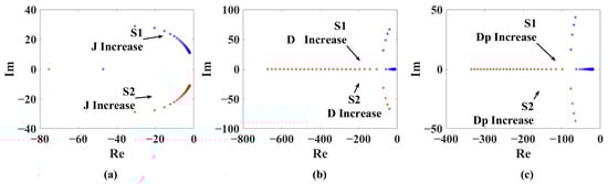
Figure 1. VSG Grid-Connected Stability Analysis: (a) Virtual Inertia J (b) Damping Coefficient D (c) Active Power Droop Coefficient $D_p$.

In summary, the fixed-parameter VSG cannot simultaneously optimize response speed and stability by adjusting a single parameter. Therefore, this paper introduces a reinforcement learning–based control strategy to enable real-time coordinated tuning of J, D, and $D_p$, improving both system stability and robustness.

2.3. VSG Parameter Design

The initial virtual inertia and damping coefficients should balance system dynamics and stability. Typically, the damping ratio is within $0.6\le \xi \le 1.0$. From (8), the natural frequency ${\omega }_n$ and damping ratio $\xi$ of the VSG system are given by

$${\omega }_n=\sqrt{{\displaystyle \frac{K_p}{J{\omega }_0}}},\xi =D\sqrt{{\displaystyle \frac{{\omega }_0}{4J{K}_p}}}+D_p\sqrt{{\displaystyle \frac{1}{4J{\omega }_0{K}_p}}}$$

(9)

and thus

$$D=2\xi \sqrt{{\displaystyle \frac{3E{U}_{\mathrm{ref}}J}{X{\omega }_0}}}-{\displaystyle \frac{D_p}{{\omega }_0}}$$

(10)

In addition, the damping coefficient is affected by the changes in mechanical torque and angular frequency, which can be approximated as

$$D={\displaystyle \frac{\Delta T}{\Delta {\omega }_{\max }}}={\displaystyle \frac{\Delta P}{\omega \Delta {\omega }_{\max }}}\approx {\displaystyle \frac{\Delta P}{{\omega }_0\Delta {\omega }_{\max }}}$$

(11)

According to the provisions of the EN50438 standard [27] regarding the grid connection of renewable energy sources, for every 1 Hz change in grid frequency, the corresponding change in the active power output of the inverter should be within 40% to 100% of the rated capacity. In this paper, $\Delta {\omega }_{max}=2\pi$, and the inverter capacity is set to 50 KW. Calculated using Equations (10) and (11), the damping coefficient D is selected within the range (13, 25.3).

Based on the constraint on the settling time of the second-order system, the real part of the system characteristic roots $S_{1,2}$ should satisfy $\mathrm{Re}\left(s_i\right)=-{\omega }_n\xi \le R_e{\left(x\right)}_{max}$. In this study, $R_e{\left(x\right)}_{max}=-30$ is adopted.

Then, by substituting Equation (9) into the above constraints, the feasible region for a specific value of D can be obtained in the $(J,D_p)$ plane. By varying D within its design range $(13, 25.3)$, a series of feasible regions are obtained, and their envelope is the region shown in Figure 2. Finally, considering the system response speed (to avoid an excessively large $D_p$), $D_p\in (2550, 6850)$ is selected, and then the corresponding $J\in (0.20, 0.59)$ is determined from Figure 2.

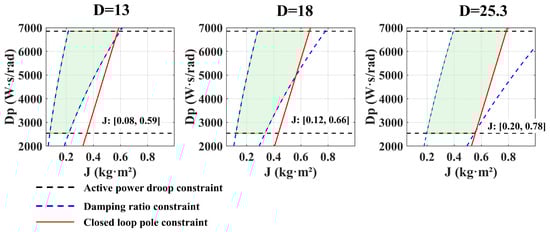
Figure 2. The ranges of J and $D_p$ under different damping coefficients.

3. VSG Multi-Parameter Collaborative Control Strategy Based on the Improved SAC-VSG

The grid-connected system employing the proposed improved SAC-VSG multi-parameter cooperative control strategy is illustrated in Figure 3. Here, $U_{dc}$ denotes the DC power supply, $L_f$ and $C_f$ are the filter inductance and filter capacitance, respectively, and $L_g$ is the grid-side inductance. The fundamental control layer consists of the active-power control loop and the reactive-power control loop. The improved part is the multi-parameter cooperative control strategy based on the improved SAC-VSG. In this strategy, the normalized angular frequency deviation $e_{\omega }$ and its derivative ${e_{\omega }}^{\prime }$, the active-power deviation $e_p$ and its derivative ${e_p}^{\prime }$, together with the transient membership vector $\overrightarrow{\mu }$ of the VSG, are fed into the agent. The agent then outputs an optimal set of virtual inertia J, damping coefficient D, and active-power droop coefficient $D_p$. These parameters are returned to the basic control layer to obtain the inverter output voltage magnitude E and the impedance angle $\theta$ of the equivalent VSG impedance. After passing through the dual voltage–current control loops and SPWM modulation, the signals are applied to the VSG main body to complete the overall closed-loop control.

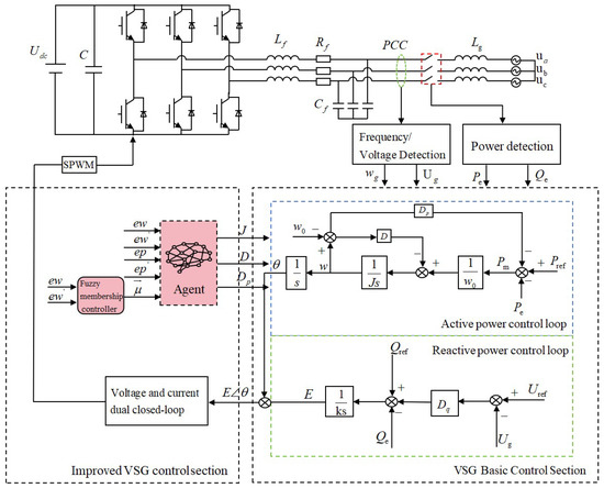
Figure 3. Multi-parameter collaborative control grid-connected system diagram based on the improved SAC-VSG.

3.1. Construction of the Fuzzy Five-Dimensional Membership Vector

3.1.1. Regional Division and Physical Meaning

When the power system is subjected to disturbances, the frequency and active-power output of the VSG experience a complete transient process. This process can generally be divided into several typical stages, each exhibiting distinct dynamic characteristics and physical significance. To enable adaptive parameter adjustment and efficient agent learning, the transient process is divided into five stages based on the frequency deviation $\Delta \omega$ and its variation trend $\Delta \omega ·\frac{d\Delta \omega }{dt}$, which are continuously represented through fuzzy membership functions.

As shown in Figure 4, when the VSG operates at the steady-state point o, a disturbance causes the power angle to jump from ${\delta }_0$ to ${\delta }_1$, moving the VSG operating point from o to a. Due to damping effects, however, the trajectory does not follow the direct path $a-o-c$ but rather the oscillatory path $a-b-c-b_1-a^{\prime }$.

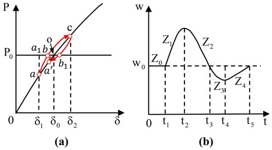
Figure 4. VSG Dynamic Adjustment Curve: (a) power angle characteristic local amplification diagram (b) angular velocity fluctuation diagram.

In the stable region $Z_0$, the system remains steady with $\Delta \omega \approx 0$ and $\frac{d\Delta \omega }{dt}\approx 0$. During the initial disturbance and acceleration stages $Z_1$ and $Z_3$, since $\Delta \omega ·\frac{d\Delta \omega }{dt}>0$ and $|\Delta \omega |$ is increasing, the system is in an acceleration phase. Therefore, J should be increased to enhance inertia, while D and $D_p$ are enlarged to suppress the frequency drop. In regions $Z_2$ and $Z_4$, where $\Delta \omega ·\frac{d\Delta \omega }{dt}<0$ and $|\Delta \omega |$ is still increasing, the system enters a deceleration phase. Here, J and $D_p$ should be reduced to accelerate frequency recovery, but this weakens damping against oscillations; hence, D must be increased to suppress overshoot.

Through the above analysis, only real-time coordinated adjustment of J, D, and $D_p$ can effectively mitigate frequency oscillations and enhance the system’s disturbance rejection. The adjustment directions of these parameters according to $\Delta \omega$ and $\Delta \omega ·\frac{\mathrm{d}\Delta \omega }{\mathrm{d}t}$ are summarized in Table 2.

Table 2. Adjustment rules for inertia J, damping coefficient D, and active droop coefficient $D_p$ under various states.

State	$\Delta \mathit{\omega }$	$\Delta \mathit{\omega }·\frac{\mathit{d}\Delta \mathit{\omega }}{\mathit{dt}}$	J	D	${\mathit{D}}_{\mathit{p}}$
$Z_0$	≈0	≈0	Unchanged	Unchanged	Unchanged
$Z_1$	>0	>0	Increase	Increase	Increase
$Z_2$	>0	<0	Decrease	Increase	Decrease
$Z_3$	<0	>0	Increase	Increase	Increase
$Z_4$	<0	<0	Decrease	Increase	Decrease

3.1.2. Design of the Membership Function

To avoid discontinuities caused by hard partitioning of transient regions, a fuzzy-partition-based five-dimensional membership vector construction method is proposed. The core idea is to map $\Delta \omega$ and $\frac{d\Delta \omega }{dt}$ into a two-dimensional feature space and apply Gaussian basis functions for soft division of the five transient regions. This yields a smooth state vector $\overrightarrow{\mu }={[{\mu }_0,{\mu }_1,{\mu }_2,{\mu }_3,{\mu }_4]}^{\mathrm{T}}$ as an auxiliary observation for the agent. The method enables smooth transitions across region boundaries, thereby improving the stability and robustness of the control strategy. The overall process is shown in Figure 5.

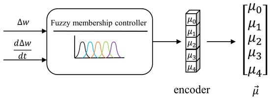
Figure 5. Flow Chart for Membership Degree Vector Design.

To ensure that different physical quantities are handled on the same scale, the frequency deviation and its rate of change are first normalized, and a coupling term e is introduced.

$$\begin{array}{cc}\hfill x& =tanh\left({\displaystyle \frac{\Delta \omega }{{\omega }_s}}\right),y=tanh\left({\displaystyle \frac{d\Delta \omega /dt}{\alpha }}\right),e=tanh\left({\displaystyle \frac{\Delta \omega ·d\Delta \omega /dt}{\beta }}\right)\hfill \end{array}$$

(12)

where ${\omega }_s$, $\alpha$, and $\beta$ are scaling factors. For each stage $(x_i,y_i)$, the unnormalized weight is defined as

$$s_i=exp\left(-{\displaystyle \frac{{(x-x_i)}^2}{2{\sigma }_x^2}}-{\displaystyle \frac{{(y-y_i)}^2}{2{\sigma }_y^2}}\right)·(1+\kappa e_{i}e)$$

(13)

where ${\sigma }_x,{\sigma }_y$ denote fuzzy widths, $\kappa$ is the coupling coefficient, and $e_i\in \{-1,0,1\}$ indicates the desired sign of $\Delta \omega ·\frac{d\Delta \omega }{dt}$ for each region. After normalization:

$${\mu }_i={\displaystyle \frac{s_i}{{\sum }_{j=0}^4(s_j+ϵ)}},\overrightarrow{\mu }=[{\mu }_0,{\mu }_1,{\mu }_2,{\mu }_3,{\mu }_4]$$

(14)

where $ϵ$ prevents division by zero and ensures ${\mu }_i\in (0, 1)$ with ${\sum }_i{\mu }_i=1$. To suppress high-frequency jitter, a first-order low-pass filter is applied:

$${\mu }_i\left[k\right]=(1-\gamma ){\mu }_i[k-1]+\gamma {\mu }_i\left[k\right],\gamma ={\displaystyle \frac{T_s}{\tau +T_s}}$$

(15)

where $T_s$ is the sampling period and $\tau =0.05$ s is the time constant.

The design of the aforementioned fuzzy parameters adheres to the following principles: the scaling factors $w_s$, $\alpha$, and $\beta$ are set according to the system’s permissible maximum frequency deviation, maximum rate of frequency change, and the typical magnitude of their product, respectively. The fuzzy widths ${\sigma }_x$ and ${\sigma }_y$ control the smoothness of regional transitions, and their values ensure a reasonable overlap between adjacent transient regions. Specific parameters are initially determined through offline analysis of typical disturbance scenarios, as detailed in Table 3. It should be emphasized that the fuzzy parameter design in this paper aims to align the region division with the physical transient characteristics of the VSG, rather than pursuing a single optimal solution. Within the reinforcement learning framework, the agent is capable of autonomously learning and adapting to different parameter configurations. Therefore, as long as the parameters remain within a reasonable physical range, the proposed control strategy can maintain stable performance.

Table 3. Fuzzy Controller Parameter Configuration.

Parameter	Value
Frequency Deviation Scaling Factor $w_s$	6.28
Frequency Change Rate Scaling Factor $\alpha$	160
Product Scaling Factor $\beta$	120
Fuzzy Width ${\sigma }_x/{\sigma }_y$	0.5
Coupling Weight Coefficient $\kappa$	0.15

3.2. Establishment of a Markov Decision Model Based on SAC with Fuzzy Membership Vector

The frequency and power oscillation problem of the VSG under disturbances is modeled as a multi-objective optimization problem. Unlike conventional single-objective methods, the proposed framework incorporates partitioned optimization objectives corresponding to different transient stages, ensuring both frequency and power dynamic performance. The parameter adjustments of the VSG are formulated as a Markov Decision Process (MDP), comprising state space, action space, and reward function [25].

3.2.1. State Space

To suppress frequency and power oscillations under disturbances while implementing stage-wise control strategies by recognizing different transient responses, the VSG state space is defined as

$$S_t=\{e_{\omega },{e_{\omega }}^{\prime },e_p,{e_p}^{\prime },\overrightarrow{\mu }\}$$

(16)

where $e_p=\frac{P_{\mathrm{ref}}-P_e}{K_p}$ and $e_{\omega }=\frac{\omega -{\omega }_0}{K_{\omega }}$, with $K_p$ and $K_{\omega }$ representing the normalization coefficients for active power and angular frequency deviation, respectively.

3.2.2. Action Space

The action vector is defined by the control variables directly adjusted by the agent, corresponding to the changes in virtual inertia, damping, and droop coefficients:

$$a_t=\left\{\Delta J,\Delta D,\Delta D_p\right\}$$

(17)

Accordingly, the actual outputs of inertia $J_t$, damping $D_t$, and droop coefficient $D_{p_t}$ re expressed as

$$\left\{\begin{array}{cc}\hfill J_t& =J_0+\Delta J_t\hfill \\ \hfill D_t& =D_0+\Delta D_t\hfill \\ \hfill D_{p_t}& =D_{p_0}+\Delta D_{p_t}\hfill \end{array}\right.$$

(18)

where $J_0$, $D_0$, and $D_{p_0}$ denote the initial values of virtual inertia, damping coefficient, and active power droop coefficient, respectively.

3.2.3. Reward Function

The reward function is designed to not only optimize the power and frequency performance but also account for the stage-specific transient behavior of the VSG. By introducing a fuzzy membership vector corresponding to the transient stages, the agent can learn differentiated optimization policies that achieve more targeted control in each phase.

• Frequency deviation penalty $pe{n}_{\omega }$:

During disturbances, smaller frequency deviations and shorter oscillation durations are preferred. The frequency penalty is defined as

$$pe{n}_{\omega }=-r_{\omega }·\left|e_{\omega }\right|$$

(19)

• Active power deviation penalty $pe{n}_P$:

Similarly, the active power is expected to fluctuate minimally around its reference and quickly return to steady state. The penalty function is given by:

$$pe{n}_P=-r_P·\left|e_P\right|$$

(20)

• Directional consistency reward $rewar{d}_{\mathrm{dir}}$:

To integrate the expert adjustment rules from Table 2 into the learning process, an expected direction matrix $E\in {\mathbb{R}}^{3\times 5}$ is constructed, encoding the expected variation trends of each parameter across different transient regions from $Z_0$ to $Z_4$.

$$E=\left[\begin{array}{ccccc}E(J,Z_0)& E(J,Z_1)& E(J,Z_2)& E(J,Z_3)& E(J,Z_4)\\ E(D,Z_0)& E(D,Z_1)& E(D,Z_2)& E(D,Z_3)& E(D,Z_4)\\ E(D_p,Z_0)& E(D_p,Z_1)& E(D_p,Z_2)& E(D_p,Z_3)& E(D_p,Z_4)\end{array}\right]$$

(21)

where $E\left(i,j\right)\in \left\{-1,0,1\right\}$ represents the expected directional tendency of each parameter (J, D, $D_p$) in stage $Z_j$. Here, ‘1’ indicates that the parameter should be increased, ‘$-1$’ indicates that it should be decreased, and ‘0’ indicates that the parameter should remain unchanged. The specific entries of matrix E are fully consistent with the rules presented in Table 2.

Given the fuzzy membership vector at the current time step, $\overrightarrow{\mu }={[{\mu }_0,{\mu }_1,{\mu }_2,{\mu }_3,{\mu }_4]}^{\mathrm{T}}$, the comprehensive expected direction vector $\overrightarrow{e_z}$ for the three parameters is computed via weighted summation as

$$\overrightarrow{e_z}=E·\overrightarrow{\mu }$$

(22)

where $\overrightarrow{e_z}={[e_J,e_D,e_{D_p}]}^{\mathrm{T}}$ represents the desired direction of variation for each parameter. The directional reward is then determined by the cosine similarity between the actual action vector $\overrightarrow{a}$ and the expected direction $\overrightarrow{e_z}$:

$$rewar{d}_{\mathrm{dir}}=r_{\mathrm{dir}}·{\displaystyle \frac{\overrightarrow{a}·\overrightarrow{e_z}}{\parallel \overrightarrow{a}\parallel \parallel \overrightarrow{e_z}\parallel }}$$

(23)

• Action smoothness penalty $pe{n}_{\mathrm{smooth}}$:

By penalizing significant differences between action values at adjacent time steps, the approach serves to constrain the rate of change for virtual inertia, damping, and droop coefficients.

$$\begin{array}{c}\hfill pe{n}_{\mathrm{smooth}}=-r_s·\sqrt{{(\Delta J_t-\Delta J_{t-1})}^2+{(\Delta D_t-\Delta D_{t-1})}^2+{(\Delta D_{p_t}-\Delta D_{p_{t-1}})}^2}\end{array}$$

(24)

Finally, the total reward is formulated as

$$Reward=pe{n}_{\omega }+pe{n}_P+rewar{d}_{\mathrm{dir}}+pe{n}_{\mathrm{smooth}}$$

(25)

The weighting of each term in the reward function is determined based on the principles of multi-objective optimization and the prioritization of system safety and stable operation. First, frequency stability is the primary objective; therefore, the penalty weight for frequency deviation $r_{\omega }$ is set to the largest value. Active power tracking is a fundamental function of the VSG, and its weight $r_p$ is assigned the second-highest value. The directional consistency reward $r_{\mathrm{dir}}$ is introduced to incorporate expert knowledge, with its weight calibrated so that its magnitude is comparable to the main penalty terms during the early stages of training. However, $r_{\mathrm{dir}}$ should not be excessively large, as it needs to allow the agent to explore appropriate values within a reasonable range. The action smoothness penalty weight $r_s$ is set relatively small to prevent overly restrictive limitations on dynamic adjustment capability while still being sufficient to suppress detrimental high-frequency oscillations.

3.3. Improved SAC-VSG Algorithm

The Soft Actor–Critic (SAC) algorithm is adopted to solve the MDP of VSG frequency optimization. Compared with conventional RL algorithms, SAC handles continuous action spaces more effectively and demonstrates superior convergence speed and training stability [28].

Figure 6 illustrates the overall architecture of the improved SAC-VSG algorithm. Compared with the traditional SAC-VSG, this framework incorporates an expert knowledge guidance module. This module first fuzzifies the real-time VSG system measurements ($\Delta \omega$, $\dot{\Delta \omega }$) into a membership degree vector $\overrightarrow{\mu }$. Then, by integrating with the expert rule matrix E from Table 2, it synthesizes an expected direction vector $\overrightarrow{e_z}$. The vector $\overrightarrow{e_z}$ is fed into the SAC agent as a soft guidance signal, encouraging the agent to output actions consistent with expert experience through the reward term $r_{\mathrm{dir}}$ (Equation (23)). Concurrently, $\overrightarrow{\mu }$ is also provided as part of the state input to the SAC agent, enabling transient region-aware perception. This design allows the algorithm to leverage expert domain knowledge to enhance interpretability while retaining the capability of reinforcement learning to autonomously explore optimal control policies.

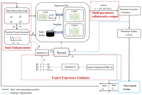
Figure 6. Schematic of the Multi-parameter Collaborative Adaptive Algorithm Based on Improved SAC-VSG.

3.3.1. Actor Network

In the improved SAC-VSG framework, the Actor network outputs the parameter set $(J_t,D_t,D_{pt})$, which are essential for the stable grid-connected operation of the VSG. The policy network, parameterized by $\varphi$, is denoted as

$${\pi }_{\varphi }\left(a\right|s)$$

(26)

and adopts a stochastic Gaussian policy. The network outputs the mean and log standard deviation to construct the action distribution. The sampled action is given by

$$a_t\sim \mathcal{N}\left(\mu \left(s\right),\sigma \left(s\right)\right)$$

(27)

To ensure differentiability during sampling, the reparameterization trick is applied:

$$x_t=\mu \left(s\right)+\sigma \left(s\right)·ϵ,ϵ\sim \mathcal{N}(0,1)$$

(28)

followed by a hyperbolic tangent squashing function:

$$a_t=tanh\left(x_t\right)$$

(29)

which guarantees that the final action lies within the normalized range $[-1, 1]$.

3.3.2. Critic Network

The Critic network evaluates state–action pairs by estimating their expected return (Q-value), thus providing gradient information for updating the Actor. A twin Q-network architecture is employed to suppress overestimation bias, where the minimum of the two Q-values is used for the target computation. The soft Q-value target follows the Bellman equation:

$$\begin{array}{c}\hfill Q^{\mathrm{target}}(s_t,a_t)=r(s_t,a_t)+\gamma \left[\underset{i=1,2}{min}{Q}_i^{\mathrm{target}}(s_{t+1},a_{t+1})-\alpha log\left({\pi }_{\varphi }\left(a_{t+1}\right|s_{t+1})\right)\right]\end{array}$$

(30)

The target network parameters are updated using Polyak averaging:

$${\varphi }_{\mathrm{target}}^{\prime }\leftarrow \tau \varphi +(1-\tau ){\varphi }_{\mathrm{target}}^{\prime }$$

(31)

where $\tau \in (0, 1)$ determines the update rate and helps maintain training stability.

3.3.3. Network Architecture

As shown in Figure 7, both the Actor network and the Critic networks employ fully connected feedforward neural networks. The specific configurations are as follows.

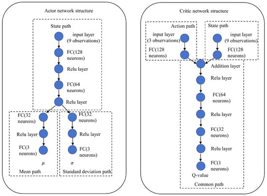
Figure 7. Actor and Critic Network Architecture Diagram.

3.3.4. Overall Process of Parameter Adjustment Control Based on the Improved SAC-VSG Strategy

Figure 8 illustrates the overall flow of the parameter adjustment control based on the improved SAC-VSG strategy. The algorithm proceeds as follows: an initial set of values for virtual inertia J, damping coefficient D, and active power droop coefficient $D_p$ is selected within their permissible ranges. These initial values, together with the VSG-connected system, are used to form the state space equations fed into the agent for training. During each episode, the agent receives a reward, which is accumulated until the cumulative reward is maximized. The optimal values of J, D, and $D_p$ derived from the agent’s policy are then subjected to amplitude-limiting and optimization, yielding the parameter values for the next time step and completing the closed-loop control.

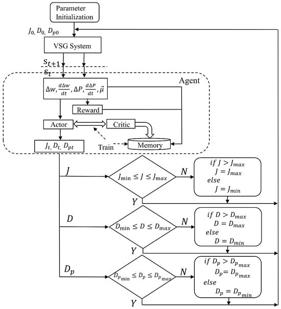
Figure 8. Flowchart for Adjusting Virtual Inertia, Damping, and Droop Coefficients.

4. Simulation Experiments and Result Analysis

To validate the effectiveness and superiority of the proposed multi-parameter adaptive control strategy based on the improved SAC-VSG (ISAC-3P VSG), a simulation model was implemented in Matlab/Simulink as shown above. The agent was developed using Reinforcement Learning Toolbox and trained under load variations, active power reference changes, and grid phase disturbances. For comparison, six VSG control strategies were evaluated: (1) multi-parameter adaptive control based on improved SAC-VSG (ISAC-3P VSG); (2) two-parameter adaptive control based on improved SAC-VSG (ISAC-2P VSG); (3) multi-parameter adaptive control based on SAC-VSG (SAC-3P VSG); (4) two-parameter adaptive control based on SAC-VSG (SAC-2P VSG); (4) two-parameter adaptive control based on DDPG-VSG (DDPG VSG); (5) conventional fixed-parameter VSG (Fixed VSG). The specific Core Characteristics differences are shown in Table 4. The simulation parameters are summarized in Table 5.

Table 4. Core Characteristics Comparison of Six VSG Control Strategies.

Control Strategy	State Space	Action Space
ISAC-3P VSG	$e_{\omega },e_{\omega }^{\prime },e_P,e_P^{\prime },\overrightarrow{\mathit{\mu }}$	$\Delta J,\Delta D,\Delta D_p$
ISAC-2P VSG	$e_{\omega },e_{\omega }^{\prime },e_P,e_P^{\prime },\overrightarrow{\mathit{\mu }}$	$\Delta J,\Delta D$
SAC-3P VSG	$e_{\omega },e_{\omega }^{\prime },e_P,e_P^{\prime }$	$\Delta J,\Delta D,\Delta D_p$
SAC-2P VSG	$e_{\omega },e_{\omega }^{\prime },e_P,e_P^{\prime }$	$\Delta J,\Delta D$
DDPG VSG	$e_{\omega },e_{\omega }^{\prime },e_P,e_P^{\prime }$	$\Delta J,\Delta D$
Fixed VSG	–	–

Table 5. VSG and grid-related control parameters.

Parameter	Value
DC-link voltage $U_{dc}$ (V)	800
Reference voltage amplitude $E_{ref}$ (V)	311
Rated frequency $f_0$ (Hz)	50
Filter inductance $L_f$ (mH)	1.5
Filter capacitance $C_f$ ($\mathrm{\mu }$F)	50
Grid-side inductance $L_g$ (mH)	1.2
virtual inertia $J_0$ (kg·m2)	0.3
damping coefficient $D_0$ (N·s·m/rad)	13
droop coefficient $D_{p0}$ ((W·s)/rad)	2550
Batch size	128
Replay buffer	100,000
Learning Rate (Actor/Critic)	3 × 10−4
Discount Factor	0.99
Soft Update Factor	0.01

As illustrated in Figure 9, the reward curves of all algorithms converge after approximately 100 training episodes. Although the ISAC-3P algorithm does not exhibit the highest final reward value, this is primarily due to its reward function incorporating a larger number of performance terms and constraint penalties, which makes the optimization objective more complex. In contrast, ISAC-3P achieves the best results in key physical performance indicators such as frequency recovery speed and overshoot, demonstrating that its overall control performance surpasses that of the other strategies. Furthermore, to evaluate the repeatability and robustness of the algorithm, this paper conducts multiple independent repeated experiments for all Reinforcement Learning (RL) control strategies. (Performance metrics are reported in the format of ‘mean ± standard deviation’. The fixed-parameter VSG strategy yields deterministic results from a single run, as it contains no stochastic elements.)

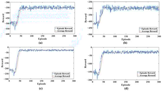
Figure 9. Training results of different algorithms: (a) ISAC-3P (b) ISAC-2P (c) SAC-3P and (d) SAC-2P.

4.1. Working Condition 1: Load Variation

Simulations were conducted using the parameters in Table 3. The total simulation duration was 1.5 s. The VSG connected to the grid at 0 s, with an initial active power reference of 10 kW. At 0.5 s, an additional 10 kW load was applied, which was removed at 1 s. Reactive power remained constant.

Table 6 presents the quantitative performance indicators for each control strategy under this condition. The metrics include maximum active power fluctuation $\Delta P_{max}$, maximum frequency deviation $\Delta f_{max}$, and system settling time $t_s$. Figure 10a shows frequency responses, while Figure 10b illustrates active power outputs.The ISAC-3P strategy demonstrates the lowest frequency overshoot, with a reduction of approximately 30.1% compared to the DDPG strategy and about 29.6% compared to the SAC-2P strategy. Its settling time is also the shortest, showcasing superior dynamic performance and disturbance rejection capability.

Table 6. Analysis indicators for different control strategies under condition 1.

Control Strategy	$\Delta {\mathit{P}}_{max}$ (kW)	$\Delta {\mathit{f}}_{max}$ (Hz)	${\mathit{t}}_{\mathit{s}}$ (s)
ISAC-3P VSG	$4.780\pm 0.015$	$0.058\pm 0.003$	$0.27\pm 0.012$
ISAC-2P VSG	$4.781\pm 0.018$	$0.072\pm 0.005$	$0.30\pm 0.015$
SAC-3P VSG	$4.782\pm 0.019$	$0.069\pm 0.006$	$0.28\pm 0.016$
SAC-2P VSG	$4.785\pm 0.021$	$0.081\pm 0.008$	$0.31\pm 0.020$
DDPG VSG	$4.784\pm 0.023$	$0.083\pm 0.010$	$0.32\pm 0.022$
Fixed VSG	$4.786$	$0.110$	$0.350$

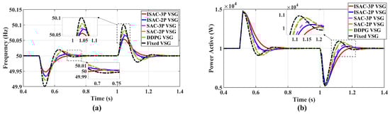
Figure 10. System responses under load variation. (a) frequency response; (b) Active power response.

As shown in Figure 11a, following the load disturbance, the dynamic evolution of the membership vector $\overrightarrow{\mu }$ clearly reveals the phased transition of the system’s transient process. After 0.5 s, ${\mu }_3$ becomes the dominant component, indicating the highest matching degree between the system state and region $Z_3$. Subsequently, the dominant membership smoothly shifts to ${\mu }_4$, and finally converges to ${\mu }_0$ (steady-state region). Notably, overlapping components exist during the transition, which reflects the soft-partitioning capability of fuzzy logic in describing continuous dynamic processes, thereby avoiding the discontinuity that could arise from traditional hard switching. The entire process aligns with the theoretical transient trajectory outlined in Table 2, demonstrating the effectiveness of the membership vector as a state perception mechanism.

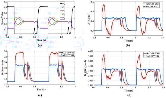
Figure 11. Parameter variations under load fluctuation: (a) Transient component value; (b) Virtual inertia; (c) Damping coefficient; (d) Active power droop coefficient.

As illustrated in Figure 11b–d, the trajectories of the virtual inertia, damping, and active-power droop coefficient reveal clear differences between the two control strategies. The ISAC strategy provides a higher virtual inertia support at the beginning of the disturbance, while simultaneously increasing the damping and active-power coefficients to suppress frequency overshoot. It then rapidly reduces the virtual inertia to accelerate frequency restoration, and leverages a relatively large damping coefficient to ensure smooth oscillation damping, thereby reducing the overshoot in both frequency and active power and shortening the recovery time.In contrast, the SAC strategy maintains relatively large parameter values after the disturbance. As analyzed earlier, excessively large inertia or active-power droop coefficients can slow down the VSG dynamic response, eventually degrading the system performance. Therefore, the ISAC strategy demonstrates superior transient performance over the SAC method. This result further verifies that incorporating the five-dimensional membership vector enables the agent to perform stage-adaptive optimization across different transient regions, effectively enhancing the overall transient performance of the VSG system.

4.2. Working Condition 2: Active Power Reference Step Change

The initial active power reference of the system was set to 0 kW. At 0.4 s, the active power reference suddenly stepped to 10 kW, and the system response was observed within 1 s.

The dynamic performance was quantitatively evaluated using the frequency deviation, active power fluctuation, and system settling time as performance indicators. The results of each strategy are summarized in Table 7. Figure 12a shows the frequency oscillation at 0.4 s under the same operating condition. The control strategy proposed in this paper (ISAC-3P) achieves the most significant reduction in system angular frequency overshoot, approximately 0.12 Hz. This represents a reduction of about 41.4% compared to the traditional strategy, about 24.5% compared to SAC-2P, and about 25% compared to DDPG. Furthermore, the ISAC-3P control strategy has the shortest settling time, demonstrating superior dynamic performance and enhanced disturbance rejection capability. Figure 12b shows that the ISAC-3P strategy yields the smallest active power overshoot, approximately 0.447 kW, which is reduced by about 1.292 kW compared to SAC-2P and by about 1.534 kW compared to DDPG. The oscillation curve is smoother, thereby improving the transient performance and stability of the system. Meanwhile, the ISAC-2P strategy produced a smaller active power overshoot than SAC-3P, indicating that the active power droop coefficient affects transient performance similarly to the damping coefficient, helping to reduce frequency and power overshoot.

Table 7. Analysis indicators for different control strategies under working condition 2.

Control Strategy	$\Delta {\mathit{P}}_{max}$ (kW)	$\Delta {\mathit{f}}_{max}$ (Hz)	${\mathit{t}}_{\mathit{s}}$ (s)
ISAC-3P VSG	$0.447\pm 0.018$	$0.120\pm 0.004$	$0.26\pm 0.008$
ISAC-2P VSG	$1.057\pm 0.032$	$0.139\pm 0.005$	$0.29\pm 0.010$
SAC-3P VSG	$0.602\pm 0.021$	$0.141\pm 0.006$	$0.28\pm 0.009$
SAC-2P VSG	$1.739\pm 0.058$	$0.159\pm 0.007$	$0.31\pm 0.012$
DDPG VSG	$1.981\pm 0.069$	$0.162\pm 0.013$	$0.32\pm 0.015$
Fixed VSG	$2.201$	$0.205$	$0.335$

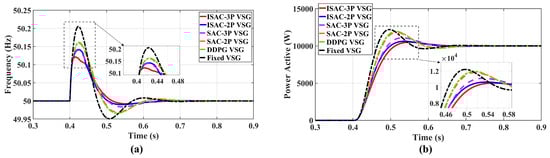
Figure 12. System responses under active power reference step change. (a) frequency response; (b) Active power response.

As shown in Figure 13a, when a step change occurs in the active power reference value, the membership vector exhibits a clear evolutionary sequence of “dominant ${\mu }_1$ → dominant ${\mu }_2$ → dominant ${\mu }_0$”. This indicates that the characteristics of the system state successively correspond mainly to regions $Z_1$ and $Z_2$, before smoothly recovering to the steady-state region $Z_0$. This result reproduces and validates the effectiveness and universality of the proposed fuzzy state-perception mechanism, demonstrating its ability to reliably identify the stages of transient processes under different types of disturbances.

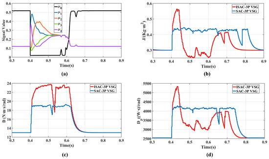
Figure 13. Parameter variations under active power reference step change: (a) Transient component value; (b) Virtual inertia; (c) Damping coefficient; (d) Active power droop coefficient.

As shown in Figure 13b–d, following the active power reference step, the ISAC strategy provides larger virtual inertia and damping support than the SAC strategy during the early disturbance stage. It then reduces the virtual inertia and active-power droop coefficient to accelerate frequency recovery, while maintaining a relatively high damping coefficient to suppress oscillations in both frequency and active power. This demonstrates that the ISAC strategy achieves a more effective trade-off among the three parameters across different transient regions, thereby improving the dynamic response speed of the VSG system.

4.3. Working Condition 3: Grid Phase Angle Disturbance

Initially, the system operates with a rated load of 10 kW, and the VSG is grid-connected. The grid phase voltage magnitude is stable at 311 V, and the frequency is approximately 50 Hz. At 0.5 s, the grid phase experiences an abrupt drop of 8°, and the system response is observed over 1 s. The dynamic performance was quantitatively evaluated using the frequency deviation, active power fluctuation, and system settling time as performance indicators. The results of each strategy are summarized in Table 8.

Table 8. Analysis indicators for different control strategies under working condition 3.

Control Strategy	$\Delta {\mathit{P}}_{max}$ (kW)	$\Delta {\mathit{f}}_{max}$ (Hz)	${\mathit{t}}_{\mathit{s}}$ (s)
ISAC-3P VSG	$3.483\pm 0.042$	$0.27\pm 0.006$	$0.27\pm 0.007$
ISAC-2P VSG	$3.480\pm 0.048$	$0.35\pm 0.009$	$0.29\pm 0.009$
SAC-3P VSG	$3.481\pm 0.050$	$0.34\pm 0.010$	$0.28\pm 0.008$
SAC-2P VSG	$3.478\pm 0.053$	$0.41\pm 0.013$	$0.31\pm 0.011$
DDPG VSG	$3.482\pm 0.057$	$0.42\pm 0.016$	$0.32\pm 0.013$
Fixed VSG	$3.475$	$0.520$	$0.336$

Figure 14a illustrates the comparison of system angular frequency responses under six control strategies. It can be observed that, during the grid phase drop, the maximum frequency deviation under traditional VSG control is 0.52 Hz, whereas the proposed ISAC-3P strategy achieves 0.27 Hz, reducing the deviation by approximately 34.1% compared with SAC-VSG . Moreover, ISAC-3P demonstrates faster frequency recovery and smoother transient response, significantly improving system transient performance.

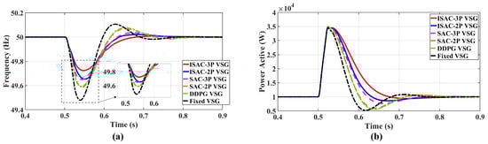
Figure 14. System responses under grid phase angle disturbance. (a) frequency response; (b) Active power response.

As shown in Figure 14b, when the grid phase drops abruptly, the VSG rapidly responds by increasing power output to maintain frequency stability. Compared with traditional VSG, SAC-VSG and DDPG-VSG control strategies, the proposed ISAC-3P VSG strategy exhibits smaller power oscillations, resulting in a smoother active power curve. This optimization allows the VSG to more smoothly handle the transient process caused by the grid phase disturbance, effectively enhancing operational robustness against external disturbances such as grid phase changes.

As shown in Figure 15a, when a phase-angle sag disturbance occurs in the grid, the membership vector accurately captures the complex evolutionary process of the system dynamics. The component ${\mu }_3$ rises rapidly and becomes dominant, indicating that the system dynamics primarily exhibit characteristics corresponding to region $Z_3$ (reverse acceleration). Subsequently, the dominant component transitions smoothly through ${\mu }_4$, ${\mu }_1$, and ${\mu }_2$, before ${\mu }_0$ finally stabilizes as the dominant component, signifying the system’s return to the steady state. This result further confirms that the proposed fuzzy-perception mechanism can continuously track the complete transient stages of the system even under complex grid disturbances.

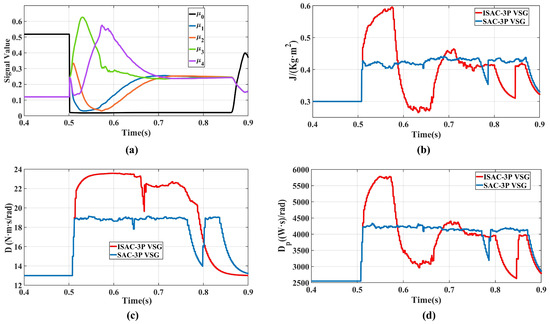
Figure 15. Parameter variations under grid phase angle disturbance: (a) Transient component value; (b) Virtual inertia; (c) Damping coefficient; (d) Active power droop coefficient.

Figure 15b–d demonstrate that both the ISAC and SAC multi-parameter control strategies are capable of maintaining stable VSG operation under the new grid conditions. As discussed earlier, the ISAC strategy can adaptively adjust each parameter across different transient regions, resulting in smaller frequency overshoot and shorter recovery time. These results clearly indicate that the proposed ISAC control strategy provides stronger dynamic adaptability and operational robustness when dealing with external disturbances.

5. Conclusions

The improved SAC-based VSG multi-parameter coordinated control strategy (ISAC-3P) integrates the advantages of fuzzy logic and reinforcement learning, achieving a state–action dual-layer optimization under the Markov decision framework. This provides a robust and disturbance-resilient control solution for renewable-energy-based power systems.

By introducing a five-dimensional fuzzy membership vector and designing a reward function that combines stage-based guidance with autonomous exploration, the controller can perform differentiated optimization according to the VSG’s transient stages, effectively improving transient response speed and oscillation suppression. Meanwhile, a multi-parameter coordinated control mechanism with feasible-region constraints was developed, enabling adaptive coordination of virtual inertia, damping, and active power droop coefficients. This achieves a balanced trade-off between power dynamics and frequency stability, further enhancing system transient performance and robustness.

The ISAC-VSG strategy demonstrates superior transient performance under multiple disturbance conditions, validating its effectiveness and advanced capabilities. However, this study has certain limitations. The validation work is primarily based on simulation models of a single grid-connected system, and its coordination performance in complex multi-machine interconnected networks requires further investigation. Future research will focus on the following directions: (1) Extending the proposed architecture to multi-machine parallel VSG systems, investigating their coordination and communication interaction mechanisms; (2) Expanding the proposed framework to other advanced DRL algorithms such as TD3 for further investigation.

References

- Zheng, H. Research on low-carbon development path of new energy industry under the background of smart grid. J. King Saud Univ.-Sci. 2024, 36, 103105. [Google Scholar] [CrossRef]
- Amjith, L.R.; Bavanish, B. A review on biomass and wind as renewable energy for sustainable environment. Chemosphere 2022, 293, 133579. [Google Scholar] [CrossRef] [PubMed]
- Chen, X.H.; Tee, K.; Elnahass, M.; Ahmed, R. Assessing the environmental impacts of renewable energy sources: A case study on air pollution and carbon emissions in China. J. Environ. Manag. 2023, 345, 118525. [Google Scholar] [CrossRef]
- Xiao, X.; Zheng, Z. New power systems dominated by renewable energy towards the goal of emission peak and carbon neutrality: Contribution, key techniques, and challenges. Adv. Eng. Sci. 2022, 54, 47. [Google Scholar]
- Chen, S.; Sun, Y.; Hou, X.; Han, H.; Fu, S.; Su, M. Quantitative parameters design of VSG oriented to transient synchronization stability. IEEE Trans. Power Syst. 2023, 38, 4978–4981. [Google Scholar] [CrossRef]
- Chen, J.; Liu, M.A.; Chen, X.; Niu, B.W.; Gong, C.Y. Wireless parallel and circulation current reduction of droop-controlled inverters. Trans. China Electrotech. Soc. 2018, 33, 1450–1460. [Google Scholar]
- Li, D.; Zhu, Q.; Lin, S.; Bian, X.Y. A self-adaptive inertia and damping combination control of VSG to support frequency stability. IEEE Trans. Energy Convers. 2017, 32, 397–398. [Google Scholar] [CrossRef]
- Lyu, Z.; Gong, X.; Liu, L.; Liu, L. Parameters analysis and operational area calculations of VSG applied to distribution networks. CSEE J. Power Energy Syst. 2023, 9, 2214–2223. [Google Scholar]
- Altawallbeh, A.; Alassi, A.; Meskin, N.; Al-Hitmi, M.A.; Massoud, A.M. Small-Signal Stability Analysis and Parameters Optimization of Virtual Synchronous Generator for Low-Inertia Power System. IEEE Access 2025, 13, 107227–107243. [Google Scholar] [CrossRef]
- Zhang, M.; Zhao, T.; Zhu, A.; Tao, Y.; Sun, Q.; Cao, Y. Control strategy of virtual synchronous generator based on current model prediction. Mach. Electron. 2023, 41, 63–69. [Google Scholar]
- He, K.; Tang, Y.; Hu, M.J.; Guo, L. LQR control strategy for virtual synchronous generator adapted to stiff grid. Electr. Power Syst. Res. 2024, 234, 100604. [Google Scholar] [CrossRef]
- Markovic, U.; Chu, Z.; Aristidou, P.; Hug, G. LQR-based adaptive virtual synchronous machine for power systems with high inverter penetration. IEEE Trans. Sustain. Energy 2019, 10, 1501–1512. [Google Scholar] [CrossRef]
- Wang, Z.; Wang, Y.; Davari, M.; Blaabjerg, F. An effective PQ-decoupling control scheme using adaptive dynamic programming approach to reducing oscillations of virtual synchronous generators for grid connection with different impedance types. IEEE Trans. Ind. Electron. 2024, 71, 3763–3775. [Google Scholar] [CrossRef]
- Li, J.; Wen, B.; Wang, H. Adaptive virtual inertia control strategy of VSG for micro-grid based on improved bang-bang control strategy. IEEE Access 2019, 7, 39509–39514. [Google Scholar] [CrossRef]
- Lyu, L.; Wang, X.; Zhang, L.; Zhang, Z.; Koh, L.H. Fuzzy control-based virtual synchronous generator for self-adaptive control in hybrid microgrid. Energy Rep. 2022, 8, 12092–12104. [Google Scholar] [CrossRef]
- Hu, Y.; Wei, W.; Peng, Y.; Lei, J. Fuzzy virtual inertia control for virtual synchronous generator. In Proceedings of the 2016 35th Chinese Control Conference (CCC), Chengdu, China, 27–29 July 2016; pp. 8523–8527. [Google Scholar]
- Wei, B.; Xia, X.; Yu, F.; Zhang, Y.; Xu, X.; Wu, H.; Gui, L.; He, G. Multiple adaptive strategies based particle swarm optimization algorithm. Swarm Evol. Comput. 2020, 57, 100731. [Google Scholar] [CrossRef]
- Guo, J.; Fan, Y. Adaptive control strategy of VSG parameters based on improved particle swarm optimization. J. Electr. Mach. Control 2022, 26, 72–82. [Google Scholar]
- Zhao, N.; Qiao, P.; Zhou, P.; Xu, X. Adaptive control strategy of VSG parameters based on improved grey wolf algorithm. Power Sci. Eng. 2024, 40, 33–43. [Google Scholar]
- Zhang, K.; Zhang, C.; Xu, Z.; Ye, S.; Liu, Q.; Lu, Z. A virtual synchronous generator control strategy with Q-learning to damp low frequency oscillation. In Proceedings of the Asia Energy and Electrical Engineering Symposium (AEEES), Chengdu, China, 28–30 March 2020. [Google Scholar]
- Wu, W.; Guo, F.; Ni, Q.; Liu, X.; Qiu, L.; Fang, Y. Deep Q-network based adaptive robustness parameters for virtual synchronous generator. In Proceedings of the IEEE Transportation Electrification Conference and Expo, Asia-Pacific (ITEC Asia-Pacific), Hangzhou, China, 28–31 October 2022; pp. 1–4. [Google Scholar]
- Skiparev, V.; Belikov, J.; Petlenkov, E. Reinforcement learning-based approach for virtual inertia control in microgrids with renewable energy sources. In Proceedings of the IEEE PES Innovative Smart Grid Technologies Europe (ISGT-Europe), Amsterdam, Netherlands, 25–28 October 2020. [Google Scholar]
- Yang, M.; Wu, X.; Loveth, M.C. A deep reinforcement learning design for virtual synchronous generators accommodating modular multilevel converters. Appl. Sci. 2023, 13, 5879. [Google Scholar] [CrossRef]
- Lu, C.; Zhuan, X. Adaptive control for virtual synchronous generator parameters based on soft actor-critic. Sensors 2024, 24, 2035. [Google Scholar] [CrossRef] [PubMed]
- Haarnoja, T.; Zhou, A.; Abbeel, P.; Levine, S. Soft actor-critic: Off-policy maximum entropy deep reinforcement learning with a stochastic actor. In Proceedings of the International Conference on Machine Learning (ICML), Stockholm, Sweden, 10–15 July 2018; pp. 1861–1870. [Google Scholar]
- Wang, Z.; Zhang, Y.; Cheng, L.; Li, G. Improved virtual synchronous control strategy with multi-parameter collaborative adaptation. Power Syst. Technol. 2023, 47, 2403–2413. [Google Scholar]
- BS EN 50438:2007; Requirements for the Connection of Micro-Generators in Parallel with Public Low-Voltage Distribution Networks. European Committee for Electrotechnical Standardization: Brussels, Belgium, 2007.
- Pan, J.; Huang, J.; Cheng, G.; Zeng, Y. Reinforcement learning for automatic quadrilateral mesh generation: A soft actor–critic approach. Neural Netw. 2023, 157, 288–304. [Google Scholar] [CrossRef] [PubMed]
Disclaimer/Publisher’s Note: The statements, opinions and data contained in all publications are solely those of the individual author(s) and contributor(s) and not of MDPI and/or the editor(s). MDPI and/or the editor(s) disclaim responsibility for any injury to people or property resulting from any ideas, methods, instructions or products referred to in the content. |
© 2025 by the authors. Licensee MDPI, Basel, Switzerland. This article is an open access article distributed under the terms and conditions of the Creative Commons Attribution (CC BY) license.